CERN-TH/2002-379
DESY 02-223
hep-ph/0212294
December 2002

rhad: a program for the evaluation of the hadronic $R$-ratio in the perturbative regime of QCD

Abstract

This paper describes the fortran program rhad which performs a numerical evaluation of the photon-induced hadronic $R$-ratio, $R(s)$, related to the cross section for electron-positron annihilation, for a given center-of-mass energy $\sqrt{s}$. In rhad the state-of-the-art perturbative corrections to $R(s)$ are implemented and the running and decoupling of the strong coupling constant and the quark masses is automatically treated consistently. Several options allow for a flexible use of the program.

PROGRAM SUMMARY

• Title of program: rhad

• Available from:
  http://www.rhad.de/

• Computer for which the program is designed and others on which it is operable: Any work-station or PC where fortran is running.

• Operating system or monitor under which the program has been tested: Alpha, Linux, Solaris

• No. of bytes in distributed program including test data etc.: $168000$

• Distribution format: ASCII

• Keywords: Hadronic $R$-ratio, perturbative QCD, electron-positron annihilation, running and decoupling of $\alpha_{s}$

• Nature of physical problem: The hadronic $R$-ratio $R(s)$ is a fundamental quantitiy in high energy physics. It is defined as the ratio of the inclusive cross section $\sigma(e^{+}e^{-}\to\mbox{hadrons})$ and the point cross section $\sigma_{pt}=4\pi\alpha^{2}/(3s)$. It is well-defined both from the experimental and the theoretical side. $R(s)$ belongs to the few physical quantities for which high-order perturbative calculations have been performed (partial results up to order $\alpha_{s}^{4}$ exist!). Mass effects from real and virtual quarks, the evolution of the $\overline{\mbox{\small MS}}$ parameters, in particular in the presence of thresholds, and other subtleties lead to fairly complex results in high orders. Thus it is important to provide a comprehensive collection of formulas in order to make them available to non-experts.

• Method of solution: rhad is a compilation of all currently available perturbative QCD corrections to the quantity $R(s)$. Several options are provided which allow for a flexible use. In addition, rhad contains routines which perform the running and decoupling of the strong coupling constant. Thus only the center-of-mass energy has to be provided in order to determine $R(s)$.

• Restrictions on the complexity of the problem: The applicability of rhad is restricted to the perturbative energy regions and does not cover the narrow and broad resonances.

• Typical running time: The typical runtime is of the order of fractions of a second.

LONG WRITE-UP

1 General structure of $R(s)$

We are considering the fully inclusive production of quark pairs in $e^{+}e^{-}$ annihilation (for a review see Ref. [1]). The tree-level diagram for this process in shown in Fig. 1 $(a)$. At leading order (LO) perturbative QCD (pQCD), the cross section as a function of the squared center-of-mass (c.m.s.) energy, $s$, has thresholds at the points $s=4m_{Q}^{2}$ with $Q=d,u,s,c,b,t$. However, close to threshold, fixed-order pQCD is no longer applicable. Below threshold, non-perturbative effects lead to the formation of bound states of the quark–anti-quark pair, which appear as more or less sharp peaks in the cross section. In our perturbative framework of charm and bottom production, these narrow resonances cannot be described, and are therefore not included in rhad. In addition, we have to spare out the region between the physical threshold $s_{Q}^{\rm low}$ and the beginning of the more or less flat continuum region at $s_{Q}^{\rm thr}$, where the cross section exhibits rapid variations. In the case of charm production, for example, the limits would be $\sqrt{s_{c}^{\rm low}}\approx 2m_{D}\approx 3.73$ GeV and $\sqrt{s_{c}^{\rm thr}}\approx 4.8$ GeV, while for bottom production they are $\sqrt{s_{b}^{\rm low}}\approx 2m_{B}\approx 10.52$ GeV and $\sqrt{s_{b}^{\rm thr}}\approx 11.2$ GeV. Even though rhad provides a numerical value in these threshold regions, one should not try to give this value any physical significance; rhad will print a warning that reminds the user of this fact.

Furthermore, we have to exclude the low-energy region, below about $\sqrt{s_{\rm min}}=1.8$ GeV, where the validity of perturbation theory is doubtful. Thus, mass effects from $u$-, $d$- and $s$-quarks are negligible, which is why we will consider these quarks as massless throughout the paper.

Instead of the cross section $\sigma(e^{+}e^{-}\to{\rm hadrons})$, we will express the results in terms of the so-called hadronic $R$-ratio,

$$\begin{split}R(s)=\frac{\sigma(e^{+}e^{-}\to{\rm hadrons})}{\sigma(e^{+}e^{-}\to\mu^{+}\mu^{-})}\,,\end{split}$$ (1)

where

$$\begin{split}\sigma(e^{+}e^{-}\to\mu^{+}\mu^{-})=\frac{4\alpha^{2}\pi}{3s}\end{split}$$ (2)

is the high-energy limit for the photon-mediated lowest order muon pair production. In this paper we concentrate on the contributions induced by photon exchange. $Z$-boson exchange is only relevant at high energies. There, however, apart from the QCD corrections, also the electro-weak corrections become important [2]; these will not be addressed in this paper. Nevertheless, rhad can be used to evaluate the vector contribution to the production of top quarks in the same way as for charm and bottom production.

We write $R(s)$ as a sum of contributions from individual quark flavors, plus a so-called singlet term:

$$\begin{split}R(s)=\sum_{Q=d,u,s,c,b,t}R_{Q}(s)+R_{\rm sing}(s)\,.\end{split}$$ (3)

The “non-singlet” contributions $R_{Q}(s)$ are all proportional to the square of the respective quark charge. The (numerically small) singlet piece $R_{\rm sing}$ appears for the first time at order $\alpha_{s}^{3}$ and will be discussed in Sect. 6.

$R_{Q}(s)$ is defined to be zero below the continuum region of $Q\bar{Q}$ production ($s_{Q}^{\rm thr}$), i.e., we do not attempt to describe the resonance regime:

$$\begin{split}R_{Q}(s<s_{Q}^{\rm thr})=0\,.\end{split}$$ (4)

Our main concern are the radiative corrections to $R_{Q}(s)$, predominantly arising from gluons exchanged between, or emitted from, the $Q\bar{Q}$ pair, but the lowest order QED effects, though very small, will also be included. Thus we write

$$\begin{split}R_{Q}(s)&=\theta(s-s^{\rm thr}_{Q})\left[\,\sum_{n\geq 0}\left(\frac{\alpha_{s}}{\pi}\right)^{n}R_{Q}^{(n)}(s)+\delta R_{Q}^{\rm QED}(s)\right]\,.\end{split}$$ (5)

This formula generally describes the QCD/QED effects to $R_{Q}(s)$, if $\delta R_{Q}^{\rm QED}(s)$ contains all contributions that vanish when electro-magnetic corrections are ignored. Both $\alpha_{s}$ and $R_{Q}^{(n)}(s)$ explicitely depend on the renormalization scale $\mu$, while $R_{Q}(s)$ is invariant under $\mu$–variation, up to and including the order of perturbation theory that is being considered.

Since the QCD corrections only affect the quarks in Fig. 1 $(a)$, the leptonic part of the diagrams can be factored out and one remains with corrections to the $\gamma Q\bar{Q}$ vertex, and real radiation of quarks and gluons. Beyond order $\alpha_{s}$, the most convenient way to evaluate the fully inclusive rate is to compute the photon self energy and relate it to the rate $\gamma^{\ast}\to Q\bar{Q}+X$ through the optical theorem, i.e., by taking the imaginary part in the time-like region of the external momentum. Explicitely,

$$\begin{split}R(s)=12\pi{\rm Im}\Pi(s+i\epsilon)\,,\end{split}$$ (6)

where

$$\begin{split}\Pi(q^{2})=\frac{1}{3q^{2}}\left(-g_{\mu\nu}+\frac{q_{\mu}q_{\nu}}{q^{2}}\right)\,\Pi_{\mu\nu}(q)\end{split}$$ (7)

is the transversal part of the photon polarization function, $\Pi_{\mu\nu}(q)$.

The different contributions to $R(s)$, as we classify them in our paper, will be illustrated by sample diagrams contributing to $\Pi(q^{2})$ in what follows. The LO terms are thus represented by Fig. 1 $(b)$. Since the imaginary part of these diagrams is obtained by the sum of all possible cuts, it includes real and virtual contributions simultaneously.

A final remark concerning the counting of loops is in order. We understand by the $n$-loop QCD contribution to $R(s)$ the sum of real and virtual corrections to order $\alpha_{s}^{n}$. Computing $R(s)$ via the optical theorem at $n$-loop level thus requires the evaluation of the imaginary part of the photon self-energy to $n+1$ loops.

2 Running and decoupling of $\alpha_{s}$ and the quark masses

As already mentioned in the previous section, the quantity $R(s)$ depends on the strong coupling constant $\alpha_{s}$, the heavy quark masses $m_{Q}$, and the renormalization scale $\mu$. All of them are specified in the subroutine parameters which is discussed in Appendix C. The dependence of $R(s)$ on $\mu$ is explicit in terms of logarithms, but also implicit as, for example, in the argument of $\alpha_{s}$. At higher orders in perturbation theory, one needs to specify the scheme in which $\alpha_{s}$ and the quark masses $m_{Q}$ are evaluated. For $\alpha_{s}$, we will always adopt the $\overline{\mbox{\small MS}}$ scheme which is commonly used in QCD calculations. Concerning the quark masses, it is generally more appropriate to use the pole mass in the energy region close to the production threshold of the quarks. On the other hand, the use of the running mass and setting $\mu^{2}=s$ resums part of the potentially large logarithms $\ln m_{Q}^{2}/s$ in the high-energy region. For this reason, rhad provides the logical parameter lmsbar that allows the user to switch between the pole and the $\overline{\mbox{\small MS}}$ mass definition for the evaluation of $R(s)$. If not stated otherwise, we denote by $m_{Q}$ a generic quark mass in what follows. In those cases where it is necessary to distinguish between the pole and $\overline{\mbox{\small MS}}$ quark mass, we denote them by $M_{Q}$ and $\bar{m}_{Q}\equiv\bar{m}_{Q}^{(n_{f})}(\mu)$, respectively. The conversion formula between $M_{Q}$ and $\bar{m}_{Q}$ is given in App. E.4, Eq. (67). The “scale-invariant” mass is defined recursively as $\bar{m}_{Q}(\bar{m}_{Q})\equiv\bar{m}_{Q}^{(n_{f})}(\bar{m}_{Q}^{(n_{f})})$, where the number of active flavors is equal to $n_{f}=4$ for charm, $n_{f}=5$ for bottom, and $n_{f}=6$ for top quarks.

If one chooses to evaluate $R(s)$ in terms of $\overline{\mbox{\small MS}}$ masses, the input required by rhad is $\alpha_{s}^{(5)}(M_{Z})$ and the scale invariant masses $\bar{m}_{Q}(\bar{m}_{Q})$ ($Q=c,b,t$). In addition, one needs to specify the renormalization scale $\mu$ and the c.m.s. energy squared, $s$. From that, rhad will determine the number of active flavors $n_{f}$, as well as the parameters $\alpha_{s}^{(n_{f})}(\mu)$ and $\bar{m}_{Q}^{(n_{f})}(\mu)$, which will be used for the evaluation of $R(s)$. As already mentioned before, a natural choice (and the default value in rhad) for the renormalization scale is $\mu^{2}=s$.

The number of active flavors is determined through the threshold variables $s_{c}^{\rm thr}$, $s_{b}^{\rm thr}$, and $s_{t}^{\rm thr}$. When $s<s_{c}^{\rm thr}$, it assumes the smallest possible value, $n_{f}=3$, and it increases by one every time one of the threshold variables is crossed, up to $n_{f}=6$ for $s>s_{t}^{\rm thr}$.

On the other hand, in the definition of $\alpha_{s}^{(n_{f})}(\mu)$ one has the freedom to choose “matching scales” $\mu_{c}$, $\mu_{b}$, and $\mu_{t}$, at which the transition from $n_{f}$ to $n_{f}\pm 1$ is performed. For example, assume that $n_{f}=4$, and the renormalization scale is set to some specific value $\mu=\bar{\mu}$. The procedure to compute $\alpha_{s}^{(4)}(\bar{\mu})$ at $n$-loop order as implemented in rhad is as follows: In a first step the renormalization group equation (RGE) for the strong coupling (here and in what follows, we refer to App. E.4 for the definition of the coefficients $\beta$, $\zeta_{g}$, $\gamma_{m}$, and $\zeta_{m}$),

$$\mu^{2}\frac{{\rm d}}{{\rm d}\mu^{2}}\frac{\alpha_{s}^{(n_{f})}(\mu)}{\pi} = \beta^{(n_{f})}\left(\alpha_{s}^{(n_{f})}(\mu)\right)\,\,=\,\,-\sum_{i=0}^{n-1}\beta_{i}^{(n_{f})}\left(\frac{\alpha_{s}^{(n_{f})}(\mu)}{\pi}\right)^{i+2}\,,$$ (8)

is solved numerically in order to obtain $\alpha_{s}^{(5)}(\mu_{b})$ from the input value $\alpha_{s}^{(5)}(M_{Z})$. The use of the decoupling relation

$$\alpha_{s}^{(n_{f}-1)}(\mu_{b}) = \left(\zeta_{g}\right)^{2}\,\alpha_{s}^{(n_{f})}(\mu_{b})$$ (9)

to $(n-1)$-loop order, leads to $\alpha_{s}^{(4)}(\mu_{b})$. Finally, applying Eq. (8) a second time gives the value for $\alpha_{s}^{(4)}(\bar{\mu})$. The described procedure is performed automatically in rhad using the subroutine rundecalpha (see App. D).

The evaluation of $\bar{m}_{Q}^{(n_{f})}(\mu)$ from the input $\bar{m}_{Q}(\bar{m}_{Q})$ proceeds completely analogously. The RGE that governs the running of the quark masses in the $\overline{\mbox{\small MS}}$ scheme reads:

$$\begin{split}\mu^{2}\,\frac{d}{d\mu^{2}}\bar{m}_{Q}^{(n_{f})}(\mu)&=\bar{m}_{Q}^{(n_{f})}(\mu)\,\gamma_{m}^{(n_{f})}\left(\alpha_{s}^{(n_{f})}(\mu)\right)=-\bar{m}_{Q}^{(n_{f})}(\mu)\,\sum_{i\geq 0}\gamma_{m,i}^{(n_{f})}\left(\frac{\alpha_{s}^{(n_{f})}(\mu)}{\pi}\right)^{i+1}\,.\end{split}$$ (10)

Combining Eqs. (8) and (10) leads to

$$\begin{split}\bar{m}_{Q}^{(n_{f})}(\mu)&=\bar{m}_{Q}^{(n_{f})}(\mu_{0})\,\frac{c(\alpha_{s}(\mu)/\pi)}{c(\alpha_{s}(\mu_{0})/\pi)}\,,\end{split}$$ (11)

with

$$\begin{split}c(x)&=x^{c_{0}}\bigg{\{}1+(c_{1}-b_{1}c_{0})\,x+\frac{1}{2}\left[(c_{1}-b_{1}c_{0})^{2}+c_{2}-b_{1}c_{1}+b_{1}^{2}c_{0}-b_{2}c_{0}\right]x^{2}\\ &+\bigg{[}\frac{1}{6}(c_{1}-b_{1}c_{0})^{3}+\frac{1}{2}(c_{1}-b_{1}c_{0})\left(c_{2}-b_{1}c_{1}+b_{1}^{2}c_{0}-b_{2}c_{0}\right)\\ &+\frac{1}{3}\left(c_{3}-b_{1}c_{2}+b_{1}^{2}c_{1}-b_{2}c_{1}-b_{1}^{3}c_{0}+2\,b_{1}b_{2}c_{0}-b_{3}c_{0}\right)\bigg{]}\,x^{3}+{\cal O}(x^{4})\bigg{\}}\,,\\ c_{i}&\equiv\frac{\gamma_{m,i}^{(n_{f})}}{\beta_{0}^{(n_{f})}}\,,\qquad b_{i}\equiv\frac{\beta_{i}^{(n_{f})}}{\beta_{0}^{(n_{f})}}\,.\end{split}$$ (12)

If $R(s)$ is evaluated at $n$-loop order, the curly bracket of Eq. (12) has to be evaluated up to, and including, the term $\propto x^{n-1}$.

The matching between $\bar{m}_{Q}^{(n_{f})}$ and $\bar{m}_{Q}^{(n_{f}-1)}$ is determined through the equation

$$\begin{split}\bar{m}_{Q}^{(n_{f}-1)}=\zeta_{m}\,\bar{m}_{Q}^{(n_{f})}\,,\end{split}$$ (13)

where the function $\zeta_{m}$ can again be found in App. E.4. The procedure for the evaluation of $\bar{m}_{Q}^{(n_{f})}(\mu)$ from the input $\bar{m}_{Q}(\bar{m}_{Q})$ in rhad is called rundecmass (see App. D).

Note that the evaluation of $\bar{m}_{Q}^{(n_{f})}(\mu)$ is only required if the user decides to use $\overline{\mbox{\small MS}}$ masses for the evaluation of $R(s)$. In this case, in parameters.f (see App. C),

      lmsbar = .true.

and the values for massc, massb, masst have to be set to the scale invariant masses $\bar{m}_{c}(\bar{m}_{c})$, $\bar{m}_{b}(\bar{m}_{b})$, $\bar{m}_{t}(\bar{m}_{t})$, respectively. If one chooses to use pole masses instead, one defines

      lmsbar = .false.

and sets massc, massb, masst equal to the on-shell masses $M_{c}$, $M_{b}$, $M_{t}$, respectively. rhad will then simply use these values throughout the calculation.

There is one exception where we do not allow a choice between on-shell and $\overline{\mbox{\small MS}}$ mass: For “power-suppressed” corrections, i.e., double-bubble diagrams that contain a heavy secondary quark loop (see Fig. 3 $(e)$ with $m_{2}\gg\sqrt{s},m_{1}$), the heavy quark mass is always inserted in the on-shell scheme. If the input for the heavy mass is provided in the $\overline{\mbox{\small MS}}$ scheme, the corresponding on-shell value is evaluated within rhad by the subroutine mms2mos (see App. D), using the proper conversion relations [3, 4, 5].

3 Notation and tree-level result

$(a)\qquad\qquad$	$(b)$

Figure 1: $(a)$ Tree-level graph for $e^{+}e^{-}\to Q\bar{Q}$. $(b)$ One-loop photon polarization function.

$(a)$	$(b)$

Figure 2: Diagrams contributing to $R(s)$ at one-loop level.

The tree level result for $R_{Q}(s)$ is part of every introductory course in quantum field theory. It reads

$$\begin{split}R_{Q}^{(0)}(s)=n_{c}\,{\cal V}_{Q}^{2}\,r_{V}^{(0)}(s,m_{Q})\,,\qquad\mbox{with}\qquad r_{V}^{(0)}(s,M_{Q})=\frac{v_{Q}}{2}(3-v_{Q}^{2})\,,\end{split}$$ (14)

where $n_{c}=3$ is the number of colors, and ${\cal V}_{Q}$ is the electric charge of the quark $Q$ in units of the proton charge. I.e.,

$$\begin{split}{\cal V}_{u}={\cal V}_{c}={\cal V}_{t}=+\frac{2}{3}\,,\qquad{\cal V}_{d}={\cal V}_{s}={\cal V}_{b}=-\frac{1}{3}\,.\end{split}$$ (15)

$v_{Q}$ denotes the quark velocity,

$$\begin{split}v_{Q}=\sqrt{1-\frac{4M_{Q}^{2}}{s}}\,,\end{split}$$ (16)

where $\sqrt{s}$ is the c.m.s. energy. Note that we define $v_{Q}$ in terms of the on-shell mass, $M_{Q}$ (see Sect. 2). This becomes relevant at higher orders, where we refer to the definition of Eq. (16).

4 One-loop result

Sample diagrams that contribute to the one-loop approximation of $R(s)$ are shown in Fig. 2. Their imaginary part has been evaluated a long time ago in the context of QED [6]. In its most compact form, the result reads

$$\begin{split}R^{(1)}_{Q}(s)=n_{c}{\cal V}_{Q}^{2}r_{V}^{(1)}(s,m_{Q})\,,\end{split}$$ (17)

with

$$\begin{split}r_{V}^{(1)}(s,M_{Q})&=C_{\rm F}\,\frac{3-v_{Q}^{2}}{2}\Bigg{[}(1+v_{Q}^{2})\left(\mbox{Li}_{2}\left(p^{2}\right)+2\mbox{Li}_{2}\left(p\right)-\ln p\ln\frac{(1+v_{Q})^{3}}{8v_{Q}^{2}}\right)\\ &+3v_{Q}\ln\frac{1-v_{Q}^{2}}{4v_{Q}}-v_{Q}\ln v_{Q}+\frac{33+22v_{Q}^{2}-7v_{Q}^{4}}{8(3-v_{Q}^{2})}\ln\frac{1+v_{Q}}{1-v_{Q}}+\frac{15v_{Q}-9v_{Q}^{3}}{4(3-v_{Q}^{2})}\Bigg{]}\,,\end{split}$$ (18)

where $p=(1-v_{Q})/(1+v_{Q})$ and $C_{\rm F}=4/3$. In the limit $v_{Q}\to 1$, one obtains $r_{V}^{(1)}=3C_{\rm F}/4$ which, after taking into account the coupling and color factors, leads to the following expression for the QED corrections:

$$\begin{split}\delta R_{Q}^{\rm QED}=n_{c}{\cal V}_{Q}^{4}\frac{3}{4}\frac{\alpha}{\pi}\,.\end{split}$$ (19)

The tree-level and one-loop functions and their correspondence in rhad are summarized in Tab. 1.

notation	in rhad	diagrams
$r_{V}^{(0)}$	rv0	Fig. 1 $(b)$
$r_{V}^{(1)}$	rv1	Fig. 2

Table 1: Contributions to $R(s)$ at tree-level and one-loop order.

5 Two-loop result

Starting from two-loop order, a general analytic expression for $R(s)$ is no longer available. Typical diagrams are shown in Fig. 3. The full set can be obtained from these diagrams by attaching the two external photon lines to the quark lines at arbitrary points. Only certain classes of diagrams have been evaluated in closed form. Nevertheless, the analytic evaluation of different kinematical limits, combined with appropriate interpolation among these limits, have resulted in extremely accurate semi-analytical approximations to the full result. Thus, for all practical purposes, the full mass dependence is available at order $\alpha_{s}^{2}$.

Two main new features occur at the two-loop level that are absent at lower orders. First, there are contributions that are due to the non-Abelian character of QCD and have no correspondence in QED. These are diagrams with a three-gluon coupling (see Fig. 3 $(c)$ and $(d)$; the four-gluon coupling occurs for the first time at three-loop order). The second new feature is that a second quark line can appear, with the effect that the result may depend on two different quark masses $m_{1}$ and $m_{2}$ (see Fig. 3 $(e)$).

It is clear that the simplest set of diagrams to evaluate are the ones with self-energy insertions in a gluon propagator, Fig. 3 $(d)$, $(e)$. In fact, the cases with massless insertions (i.e., gluons and massless quarks) are known in closed analytical form, for general values of $s$ and $m_{1}$ [7, 8]. The same is true for $m_{1}=0$, $m_{2}\neq 0$ [9] (labels in accordance with Fig. 3 $(e)$). The case $m_{1}=m_{2}$ is known in terms of a two-dimensional integral representation [7, 10]. For $m_{1}\ll m_{2}$, the coefficient of the leading term in an expansion around $s/m_{2}^{2}\to 0$ is known in closed form [11]. For $m_{1}=0$ [12], this term was shown to approximate the exact $s/m_{2}^{2}$ dependence [9] extremely well, even up to the threshold $s=4m_{2}^{2}$.

The diagrams without self-energy insertions on gluon lines have not yet been evaluated in closed form for general values of $m_{Q}$ and $s$. The massless limit has been known for quite some time [13]. Subsequently, mass corrections in the high energy limit have been computed: The $m_{Q}^{2}/s$ terms can be obtained by a simple Taylor expansion of the integrand [14]; the $m_{Q}^{4}/s^{2}$ terms were derived from the $\overline{\mbox{\small MS}}$ operator product expansion of $\Pi(q^{2})$, combined with renormalization group relations [15]; and the evaluation of the higher order terms (up to $m_{Q}^{12}/s^{6}$) was achieved by systematically expanding the Feynman integrals [16].

However, one should note that the convergence of such a high-energy expansion is not guaranteed below the highest threshold of the diagrams under consideration. For example, the non-planar diagram in Fig. 3 $(b)$ has a four-quark cut at $q^{2}=(4m_{Q})^{2}$, meaning that the expansion around $m_{Q}^{2}/s\to 0$ formally converges only above $s=(4m_{Q})^{2}$. Nevertheless, in practice one often observes also satisfactory convergence below the threshold [16].

A result that is valid in the full kinematic range was obtained in Ref. [17] (see also Ref. [18]). To this aim, the high-energy limit was combined with up to eight moments of the polarization function obtained through an expansion for $q^{2}\to 0$. This information was combined with additional input from the threshold region around $q^{2}=4m_{Q}^{2}$, using a conformal mapping and Padé approximation in order to arrive at a three-loop expression for $\Pi(q^{2})$. For all known practical applications, this approximate result is equivalent to an analytic expression for $\Pi(q^{2})$ and, after taking the imaginary part, for $R(s)$.

Let us now explicitely parameterize the two-loop contribution to $R(s)$. We can write

$$\begin{split}R_{Q}^{(2)}(s)=n_{c}\,{\cal V}_{Q}^{2}\,\bigg{[}&r_{V}^{\rm F}(s,m_{Q})+r_{V}^{\rm A}(s,m_{Q})+\sum_{q}r_{V}^{\rm db}(s,m_{Q},m_{q})\bigg{]}\,,\end{split}$$ (20)

where the sum runs over all quark flavors. $r_{V}^{\rm F}\propto C_{\rm F}^{2}$ denotes contributions from Abelian diagrams, $r_{V}^{\rm A}\propto C_{\rm A}C_{\rm F}$ comes from non-planar and non-Abelian diagrams, and $r_{V}^{\rm db}\propto C_{\rm F}T$ (“double-bubble”) arises from diagrams with two separate quark lines. $C_{\rm F}=4/3$, $C_{\rm A}=3$ and $T=1/2$ are color factors of QCD. For later reference, it is convenient to introduce additional functions that refer to specific limits of $r_{V}^{\rm db}$:

$$\begin{split}r_{V}^{\rm db}(s,m_{Q},0)&\equiv r_{V}^{\rm L}(s,m_{Q})\,,\qquad r_{V}^{\rm db}(s,m_{Q},m_{Q})\equiv r_{V}^{\rm T}(s,m_{Q})\,.\end{split}$$ (21)

See also Tab. 2 for more details. Note that $r_{V}^{\rm db}$ introduces contributions from secondary quarks $q$ other than $Q$, both virtual and real. They arise through the splitting of gluons into a quark–anti-quark pair.

In the massless case, one has the simple expressions

$$\begin{split}r_{V}^{\rm F}(s,m_{Q}=0)&=C_{\rm F}^{2}\,\left(-\frac{3}{32}\right)\,,\\ r_{V}^{\rm A}(s,m_{Q}=0)&=C_{\rm A}C_{\rm F}\left(\frac{123}{32}-\frac{11}{4}\,\zeta_{3}-\frac{11}{16}\,L_{s\mu}\right)\,,\\ r_{V}^{\rm db}(s,m_{1}=0,m_{2}=0)&=C_{\rm F}T\left(-\frac{11}{8}+\zeta_{3}+\frac{1}{4}\,L_{s\mu}\right)\,.\end{split}$$ (22)

where $L_{s\mu}\equiv\ln(s/\mu^{2})$ and $\zeta_{3}\approx 1.20206$. The expressions in the massive case are given in App. E.1.

In the following, the expressions adopted for the individual contributions are described, and their origin is given.

• For $r_{V}^{\rm F}(s,m_{Q})$ and $r_{V}^{\rm A}(s,m_{Q})$ we use the full mass dependence as given by the Padé results of Eqs. (36), (39) [17].

• For the double-bubble contribution $r_{V}^{\rm db}(s,m_{1},m_{2})$, we have to distinguish several cases:

  • $m_{1}=m_{2}=m_{Q}$: For $\sqrt{s}\leq 4m_{Q}$, we use the analytic formula as given in Eq. (44) [7]. For $\sqrt{s}>4m_{Q}$, the full mass dependence is known in terms of a two-fold integral representation, see Eq. (46) [7]. For the sake of speed, however, we use the high energy expansion of Eq. (48) [16]. Numerical differences to the integral representation are completely negligible. Nevertheless, the user may switch to the integral formula by setting lrvctexp = .false. in rhad.

  • $m_{2}<m_{1}$: We apply an expansion for $m_{2}^{2}\ll m_{1}^{2}(<s/4)$:

    1. At ${\cal O}(m_{2}^{0})$, the full $m_{1}$-dependence is used in the form of the analytic result of Eq. (41) (for $x={\rm L}$) [7].

    2. At ${\cal O}(m_{2}^{2})$, we neglect the $m_{1}$ dependence. It turns out that this contribution vanishes which can be seen in Eq. (52).

    3. Higher orders in $m_{2}$ are neglected.

  • $(2m_{1})^{2}<s<(2m_{2})^{2}$: If $m_{1}=0$, we use the analytical result of Eq. (49) [9], including the full dependence on $m_{2}$. If $m_{1}\neq 0$, we use the leading term in $1/m_{2}^{2}$, keeping its full $m_{1}^{2}$ dependence, see Eq. (54). This expression has been obtained in Ref. [11].

  • $(2m_{1})^{2}<(2m_{2})^{2}<s$: If $m_{1}=0$, we use the analytical result of Eq. (49) [9], including the full dependence on $m_{2}$. If $m_{1}\neq 0$, we apply an expansion in the limit $m_{1}^{2}\ll m_{2}^{2}(<s/4)$:

    1. At ${\cal O}(m_{1}^{0})$, we use the analytical result of Eq. (49) [9] for the full $m_{2}$ dependence.

    2. At ${\cal O}(m_{1}^{2})$, we neglect all effects from non-zero $m_{2}$. The corresponding expression for $r_{V}^{\rm db}(s,m_{1},0)$ is given in Eq. (LABEL:eq::rvdbm1).

    3. Higher orders in $m_{1}$ are neglected.

Note that we set the ratios $m_{c}^{2}/m_{t}^{2}$ and $m_{b}^{2}/m_{t}^{2}$ to zero and consider mass corrections due to the presence of an additional light quark only for $c$-quark effects in $b$-quark production.

For the sake of completeness, let us remark that also the two-loop corrections of order $\alpha\alpha_{s}$ and order $\alpha^{2}$ for massless quarks [19] are known. Numerically, these contributions are very small. Nevertheless, we include the mixed corrections of order $\alpha\alpha_{s}$ into rhad, which modifies Eq. (19) to

$$\begin{split}\delta R_{Q}^{\rm QED}=n_{c}{\cal V}_{Q}^{4}\frac{3}{4}\frac{\alpha}{\pi}\left(1-\frac{1}{3}\frac{\alpha_{s}(\mu)}{\pi}\right)\,.\end{split}$$ (23)

Higher order QED or mixed QED/QCD effects are numerically irrelevant and will be neglected [20].

$(a)$	$(b)$	$(c)$

$(d)$	$(e)$

Figure 3: Classes of diagrams contributing to $R(s)$ at two-loop level. (For the issue of counting loops, see the discussion at the end of Sect. 1.)

notation	in rhad	diagrams	$m_{1}$	$m_{2}$
$r_{V}^{\rm F}$	rvcf	$(a)$, $(b)$	$m_{Q}$	–
$r_{V}^{\rm A}$	rvca	$(b)$, $(c)$, $(d)$	$m_{Q}$	–
$r_{V}^{{\rm db}}$	rvdb	$(e)$	$m_{1}$	$m_{2}$
$r_{V}^{\rm L}$	rvnl	$(e)$	$m_{Q}$	$0$
$r_{V}^{\rm T}$	rvct	$(e)$	$m_{Q}$	$m_{Q}$

Table 2: Different contributions to $R(s)$ at two-loop order. The column “diagrams” refers to Fig. 3, where a sample diagram is shown for each class.

6 Three-loop result

$(a)$	$(b)$	$(c)$	$(d)$

Figure 4: Classes of diagrams contributing to $R(s)$ at three-loop level.

notation	in rhad	diagrams	$m_{1}$	$m_{2}$	$m_{3}$
$r_{V}^{(3)}$	rv3	$(a)$, $(b)$, $(c)$	$m_{Q}$	$m_{Q}$ or 0	$m_{Q}$ or 0
$\delta r_{0}^{(3)}$	delr03	$(b)$, $(c)$	0	$m_{Q}$	$m_{Q}$ or 0
$r_{V,\rm sing}^{(3)}$	rv3sing	$(d)$	$m_{1}$	$m_{2}$	–

Table 3: Different contributions to $R(s)$ at three-loop order (as far as available). The column “diagrams” refers to Fig. 4, where a sample diagram is shown for each contribution.

At order $\alpha_{s}^{3}$, a new class of diagrams contributes to $R_{\rm had}$, the so-called “singlet diagrams.” They differ from the non-singlet diagrams in the sense that, in the singlet case, the external currents are not connected by a common quark line. A typical diagram is shown in Fig. 4 $(d)$. The non-singlet diagrams (see Fig. 4 $(a)$–$(c)$) are numerically dominant, but rhad includes both contributions. We will describe them in more detail in what follows.

6.1 Non-singlet contributions

The knowledge of $R(s)$ at three-loop level is restricted to the high energy limit. The massless limit was obtained for the first time in Ref. [21] and later confirmed through an independent calculation in Ref. [22].

Mass corrections are known up to ${\cal O}(m_{Q}^{4}/s^{2})$: The quadratic terms were obtained from renormalization group identities [23], while the quartic mass terms were evaluated by applying the methods of Ref. [15] at three-loop level [24].

Let us briefly discuss how we treat mass effects from massive inner quark loops. At three-loop level, there can be three different quark types in one diagram, with, say $m_{1}>m_{2}>m_{3}$. The approximation that we apply is to take all terms including $m_{1}^{4}$ and $m_{2}^{2}$, neglecting mixed terms of order $m_{1}^{2}m_{2}^{2}$. Mass effects from $m_{3}$ are also neglected. In addition, we do not consider power-suppressed terms, i.e. diagrams that contain a quark $q$ with $s<s_{q}^{\rm thr}$.

With these approximations in mind, we can write the three-loop contribution as

$$\begin{split}R_{Q}^{(3)}(s)&=n_{c}\,{\cal V}_{Q}^{2}\,\bigg{[}r_{V}^{(3)}(s,m_{Q},n_{f})+\sum_{q\neq Q}\,\delta r_{0}^{(3)}(s,m_{q},n_{f})\bigg{]}\,.\end{split}$$ (24)

$\delta r_{0}^{(3)}(s,m_{q},n_{f})$ denotes the mass corrections due to massive inner quark loops different from $Q$. According to the approximations above, it vanishes for $s<s_{q}^{\rm thr}$ and also for $m_{q}=0$.

Note that $n_{f}$ itself depends on the c.m.s. energy. Assume, for example, that $s<s_{c}^{\rm thr}$. Then we have $n_{f}=3$ and

$$\begin{split}R_{Q}^{(3)}(s)&=n_{c}\,{\cal V}_{Q}^{2}\,r_{V}^{(3)}(s,0,3)\,,\qquad Q=u,d,s\,.\end{split}$$ (25)

For $s_{c}^{\rm thr}<s<s_{b}^{\rm thr}$, we have $n_{f}=4$ and thus the non-zero contributions are

$$\begin{split}R_{Q}^{(3)}(s)&=n_{c}\,{\cal V}_{Q}^{2}\,\bigg{[}r_{V}^{(3)}(s,0,4)+\delta r_{0}^{(3)}(s,m_{c},4)\bigg{]}\,,\qquad Q=u,d,s,\\ \mbox{and}\qquad R_{c}^{(3)}(s)&=n_{c}\,{\cal V}_{c}^{2}\,r_{V}^{(3)}(s,m_{c},4)\,.\end{split}$$ (26)

For $s_{b}^{\rm thr}<s<s_{t}^{\rm thr}$, it is $n_{f}=5$ and

$$\begin{split}R_{Q}^{(3)}(s)&=n_{c}\,{\cal V}_{Q}^{2}\,\bigg{[}r_{V}^{(3)}(s,0,5)+\delta r_{0}^{(3)}(s,m_{c},5)+\delta r_{0}^{(3)}(s,m_{b},5)\bigg{]}\,,\qquad Q=u,d,s,\\ R_{c}^{(3)}(s)&=n_{c}\,{\cal V}_{c}^{2}\,\bigg{[}r_{V}^{(3)}(s,m_{c},5)+\delta r_{0}^{(3)}(s,m_{b},5)\bigg{]}\,,\\ R_{b}^{(3)}(s)&=n_{c}\,{\cal V}_{b}^{2}\,\bigg{[}r_{V}^{(3)}(s,m_{b},5)+\delta r_{0}^{(3)}(s,m_{c},5)\bigg{]}\,.\end{split}$$ (27)

Finally, for $s>s_{t}^{\rm thr}$, all masses except for $m_{t}$ are neglected, and, with $n_{f}=6$, we have

$$\begin{split}R_{Q}^{(3)}(s)&=n_{c}\,{\cal V}_{Q}^{2}\,\bigg{[}r_{V}^{(3)}(s,0,6)+\delta r_{0}^{(3)}(s,m_{t},6)\bigg{]}\,,\qquad Q=u,d,c,s,b,\\ R_{t}^{(3)}(s)&=n_{c}\,{\cal V}_{t}^{2}\,r_{V}^{(3)}(s,m_{t},6)\,.\end{split}$$ (28)

As mentioned before, in Eq. (27) it is understood that all $c$-quark mass effects are included only at ${\cal O}(m_{c}^{2})$.

The expressions for $r_{V}^{(3)}(s,m_{Q},n_{f})$ and $\delta r_{0}^{(3)}(s,m_{Q},n_{f})$ are listed in App. E.2.

6.2 Singlet contributions

As already mentioned above, singlet diagrams are characterized by the fact that each of the external photons couples to a separate quark line (see, e.g., Fig. 4 $(d)$). The singlet contribution arises first at three-loop level; at two-loop level, where the two quark lines are connected by only two gluons, it is zero due to Furry’s theorem.

We write the singlet contribution to $R(s)$ in the following way:

$$\begin{split}R_{\rm sing}(s)&=n_{c}\,\sum_{q,q^{\prime}}{\cal V}_{q}\,{\cal V}_{q^{\prime}}\,r^{(3)}_{V,\rm sing}(s,m_{q},m_{q^{\prime}})\,,\end{split}$$ (29)

where the sum over $q$ and $q^{\prime}$ runs over all active quark flavors. E.g., for $\sqrt{s}=12$ GeV it includes all quarks except for the top quark. Again, only the high energy expansion is known. Quadratic mass terms are absent, and the expression including quartic mass terms reads:

$$\begin{split}r^{(3)}_{V,\rm sing}(s,m_{1},m_{2})&=\frac{55}{216}-\frac{5}{9}\,\zeta_{3}+\frac{m_{1}^{4}}{s^{2}}\left(-\frac{10}{9}+\frac{25}{3}\,\zeta_{3}\right)+\frac{m_{2}^{4}}{s^{2}}\left(-\frac{10}{9}+\frac{25}{3}\,\zeta_{3}\right)\,.\end{split}$$ (30)

Note that, if $m_{1}\neq m_{2}$, we neglect the lighter of the two masses. Since this is the lowest order where singlet terms occur, Eq. (30) is the same in the $\overline{\mbox{\small MS}}$ and in the on-shell mass scheme.

7 Four-loop result

The knowledge of the four-loop contribution to $R(s)$ is very limited. Only contributions of diagrams with two and three quark-loop insertions have been calculated. Sample diagrams are shown in Fig. 5 $(c)$ and $(d)$. The mass effects are evaluated up to order $m_{Q}^{2}/s$, so that the results are strictly only valid in the high-energy limit.

$(a)$	$(b)$	$(c)$	$(d)$

Figure 5: Classes of diagrams contributing to $R(s)$ at four-loop level.

We write the four-loop contribution as

$$\begin{split}\bar{R}_{Q}^{(4)}(s)&=n_{c}\,{\cal V}_{Q}^{2}\,\bar{r}_{V}^{(4)}(s,m_{Q})\,,\end{split}$$ (31)

with

$$\begin{split}\bar{r}_{V}^{(4)}(s,m_{Q})&=\bar{r}_{0}^{(4),{\rm 0L}}(s)+n_{f}\,\bar{r}_{0}^{(4),{\rm 1L}}(s)+n_{f}^{2}\,r_{0}^{(4),{\rm 2L}}(s)+n_{f}^{3}\,r_{0}^{(4),{\rm 3L}}(s)\\ &+\frac{m_{Q}^{2}}{s}\left(\bar{r}_{V,2}^{(4),{\rm 0L}}(s)+n_{f}\,\bar{r}_{V,2}^{(4),{\rm 1L}}(s)+n_{f}^{2}\,r_{V,2}^{(4),{\rm 2L}}(s)+n_{f}^{3}\,r_{V,2}^{(4),{\rm 3L}}(s)\right)\,,\end{split}$$ (32)

where the bar indicates that the expressions are estimates rather than approximations or even exact results. $n_{f}$ is the number of active flavors, varying with the c.m.s. energy as discussed in Sect. 2.

$r_{0}^{(4),{\rm 3L}}$ is the renormalon-type contribution with three massless quark insertions on the gluon propagator, see Fig. 5 $(d)$. It has been evaluated in Ref. [25], where the general structure of the terms of order $\alpha_{s}(\alpha_{s}n_{f})^{n}$ was derived. Recently, the analytic expression for $r_{0}^{(4),{\rm 2L}}$ became available [26]. It required the evaluation of massless four-loop two-point functions in combination with the method of Ref. [22] (see also Ref. [18]) to derive the imaginary part of the five-loop contributions as shown in Fig. 5 $(c)$. The same method has been used in combination with the technique derived in Ref. [23] for the computation of the quadratic mass corrections $r_{V,2}^{(4),{\rm 2L}}$ and $r_{V,2}^{(4),{\rm 3L}}$ [27].

Estimates for the full massless four-loop result have been known before and are still a subject of interest [28, 29, 30]. We determine $\bar{r}_{0}^{(4)}(s)$ and $\bar{r}_{0}^{(4),{\rm L}}(s)$ by subtracting the known $n_{f}^{2}$ and $n_{f}^{3}$ contributions from the estimates of Ref. [28] at $n_{f}=1,\ldots,6$, and fitting the resulting six “data points” by a linear function in $n_{f}$. One finds, for $\mu^{2}=s$,

$$\begin{split}\bar{r}_{0}^{(4),{\rm 0L}}(s)&=-1.86\cdot 10^{2}\,,\qquad\bar{r}_{0}^{(4),{\rm 1L}}(s)=21.3\,,\\ r_{0}^{(4),{\rm 2L}}(s)&=-7.97\cdot 10^{-1}\,,\qquad r_{0}^{(4),{\rm 3L}}(s)=2.15\cdot 10^{-2}\,.\end{split}$$ (33)

The logarithmic contributions follow from the lower order terms through renormalization group invariance and are collected in App. E.3. Once the exact results for $r_{0}^{(4),{\rm 0L}}$ and $r_{0}^{(4),{\rm 1L}}$ become available, the approximate ones can easily be replaced in rhad.

Using the same method for the quadratic mass terms in combination with the estimates of Ref. [27] we obtain, in the $\overline{\mbox{\small MS}}$ scheme

$$\begin{split}\bar{r}_{V,2}^{(4),{\rm 0L}}(s)&=7.11\cdot 10^{3}\,,\qquad\bar{r}_{V,2}^{(4),{\rm 1L}}(s)=-1.43\cdot 10^{3}\,,\\ r_{V,2}^{(4),{\rm 2L}}(s)&=49.1\,,\qquad r_{V,2}^{(4),{\rm 3L}}(s)=-0.204\,.\end{split}$$ (34)

In App. E.3, the corresponding result for on-shell quark masses is listed together with the logarithmic contributions.

For completeness, the function implemented in rhad is listed in Tab. 4. Note that at ${\cal O}(\alpha_{s}^{4})$, the corrections analoguous to $\delta r_{0}^{(3)}$ are neglected.

notation	in rhad
$r_{V}^{(4)}$	rv4

Table 4: Contribution to $R(s)$ at four-loop order.

8 Evaluating $R(s)$

In this section we describe how rhad evaluates $R(s)$ in the individual energy regions. Let us first recall that $s_{Q}^{\rm thr}$ defines the lowest value of the c.m.s. energy squared, $s$, at which the perturbative treatment of $Q\bar{Q}$ production is allowed; $R_{Q}(s)$ is defined to be zero for $s<s_{Q}^{\rm thr}$. The physical threshold for $Q\bar{Q}$ production is at $s_{Q}^{\rm low}$; the user is advised, however, to disregard the results of rhad in the region between $s_{Q}^{\rm low}$ and $s_{Q}^{\rm thr}$ ($Q=c,b,t$).

The evaluation of the number of active flavors $n_{f}$, the strong coupling constant $\alpha_{s}^{(n_{f})}(\mu)$, and, if required, the $\overline{\mbox{\small MS}}$ quark masses $\bar{m}_{Q}^{(n_{f})}(\mu)$, from the input values $s$, $\mu$, $\alpha_{s}^{(5)}(M_{Z})$, and $\bar{m}_{Q}(\bar{m}_{Q})$, has been described in Sect. 2. Let us now look in more detail at the specific contributions that enter $R(s)$ at certain values of $s$.

For $s<s_{c}^{\rm low}$, i.e., below the production threshold for two $D_{0}$ mesons, we have $n_{f}=3$. The charm, bottom and top quark masses are decoupled and thus their contribution goes like $\alpha_{s}^{2}\,s/m_{q}^{2}$ ($q=c,b,t$), see Eqs. (49,54). All other correction terms are evaluated in the massless limit.

In the region $s_{c}^{\rm thr}<s<s_{b}^{\rm low}$ one has $n_{f}=4$. $\alpha_{s}^{(4)}(\mu)$ is evaluated from the input $\alpha_{s}^{(5)}(M_{Z})$, and, in the $\overline{\mbox{\small MS}}$ mass scheme, $\bar{m}_{c}^{(4)}(\mu)$ is obtained from the input quantity $\bar{m}_{c}(\bar{m}_{c})$ (see Sect. 2). In the on-shell mass scheme, the input value $M_{c}$ is used unchanged throughout the calculation. The full charm quark mass dependence (inasmuch it is known) is taken into account. Bottom and top quark are decoupled and enter through the power-suppressed terms, Eqs. (49,54), at order $\alpha_{s}^{2}$.

At c.m.s. energies above $s_{b}^{\rm thr}$ and below $s_{t}^{\rm low}$, the situation is similar to the previously described region, but with $n_{f}=5$. Note, however, that in the $\overline{\mbox{\small MS}}$ scheme not only $\bar{m}_{b}^{(5)}(\mu)$ is needed for the numerical evaluation, but also $\bar{m}_{c}^{(5)}(\mu)$. It is obtained from the input $\bar{m}_{c}(\bar{m}_{c})$ using the routine rundecmass (see Sect. D).

For $s>s_{t}^{\rm thr}$, $\alpha_{s}^{(6)}(\mu)$ and $\bar{m}_{t}^{(6)}(\mu)$ are needed for the evaluation of $R(s)$. At these energies, no mass corrections from lighter quarks are considered.

Tab. 5 and 6 show the results for $R(s)$ with the default settings (see Sect. C), for different values of the c.m.s. energy. The individual rows correspond the different orders of perturbation theory. In the case of $\sqrt{s}=5$ GeV and $\sqrt{s}=12$ GeV, we also show the partial contributions to $R(s)$ arising from massive quarks. The second column contains the value of $\alpha_{s}^{(n_{f})}(\sqrt{s})$, with the appropriate $n_{f}$.

$\sqrt{s}=2$ GeV order $\alpha_{s}$ $R(s)$ 0 0.1180 2.0012 1 0.2726 2.1747 2 0.2981 2.2223 3 0.2984 2.2049 4 0.2973 2.1835

$\sqrt{s}=5$ GeV order $\alpha_{s}$ $R_{c}(s)$ $R(s)$ 0 0.1180 1.2199 3.2220 1 0.2025 1.4956 3.6267 2 0.2120 1.5950 3.7467 3 0.2123 1.5825 3.7272 4 0.2122 1.5467 3.6867

Table 5: Hadronic $R$-ratio at $\sqrt{s}=2$ GeV ($n_{f}=3$, left) and $\sqrt{s}=5$ GeV ($n_{f}=4$, right). Note the change in $\alpha_{s}$ which is consistently evaluated from $\alpha_{s}^{(5)}(M_{Z})$. The parameter settings are given in App. C.2.

$\sqrt{s}=12$ GeV
order	$\alpha_{s}$	$R_{c}(s)$	$R_{b}(s)$	$R(s)$
0	0.1180	1.3304	0.2675	3.6001
1	0.1667	1.4199	0.3496	3.8778
2	0.1706	1.4269	0.3803	3.9265
3	0.1709	1.4198	0.3797	3.9148
4	0.1709	1.4158	0.3756	3.9050

Table 6: Hadronic $R$-ratio at $\sqrt{s}=12$ GeV ($n_{f}=5$).

Tab. 7 contains the results for $\alpha_{s}(s)$, $R(s)$, $R_{c}(s)$ and $R_{b}(s)$ for the energy region between $\sqrt{s}=1.8$ GeV and $\sqrt{s}=20$ GeV, sparing out those parts where perturbation theory is not applicable. We adopted the default values of rhad given in App. C with iord = 4. In Fig. 6 the data for $R(s)$ (full curve) are shown in graphical form. The shaded bands mark the uncertainty of $R(s)$ induced by the variation of $\alpha_{s}(M_{Z})$, $\mu$, $M_{c}$ and $M_{b}$ in the range

$$\alpha_{s}(M_{Z}) = 0.118\pm 0.003\,,$$

$$M_{c} = (1.65\pm 0.15)~{}\mbox{GeV}\,,$$

$$M_{b} = (4.75\pm 0.2)~{}\mbox{GeV}\,,$$

$$\mu \in \left[\frac{\sqrt{s}}{2},2\sqrt{s}\right]\,.$$ (35)

$\sqrt{s}$ (GeV)	$\alpha_{s}(s)$	$R_{c}(s)$	$R_{b}(s)$	$R(s)$
1.80	0.3148	0.0000	0.0000	2.1895
2.20	0.2833	0.0000	0.0000	2.1780
2.60	0.2620	0.0000	0.0000	2.1684
3.00	0.2463	0.0000	0.0000	2.1607
3.40	0.2342	0.0000	0.0000	2.1544
3.73	0.2260	0.0000	0.0000	2.1499
4.80	0.2150	1.5681	0.0000	3.7097
5.00	0.2122	1.5467	0.0000	3.6867
6.00	0.2007	1.4842	0.0000	3.6174
7.00	0.1919	1.4556	0.0000	3.5836
8.00	0.1850	1.4399	0.0000	3.5637
9.00	0.1793	1.4301	0.0000	3.5505
10.00	0.1744	1.4235	0.0000	3.5410
10.52	0.1722	1.4209	0.0000	3.5371
11.20	0.1736	1.4186	0.3793	3.9133
12.00	0.1709	1.4158	0.3756	3.9050
13.00	0.1679	1.4129	0.3717	3.8964
14.00	0.1652	1.4106	0.3685	3.8891
15.00	0.1628	1.4087	0.3659	3.8830
16.00	0.1606	1.4070	0.3636	3.8778
17.00	0.1586	1.4056	0.3618	3.8732
18.00	0.1567	1.4044	0.3602	3.8692
19.00	0.1550	1.4033	0.3589	3.8657
20.00	0.1534	1.4023	0.3577	3.8626

Table 7: $\alpha_{s}(s)$, $R_{c}(s)$, $R_{b}(s)$, and $R(s)$ for various values of $s$.

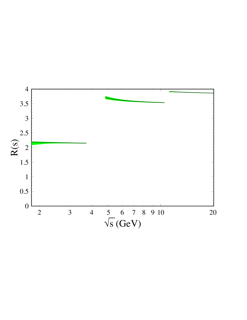
Figure 6: $R(s)$ for $1.8$ GeV $<\sqrt{s}<20$ GeV. The central curve (solid line) is obtained using the default values specified in App. C and corresponds to the results given in Tab. 7. The error bands are obtaind by varying $\alpha_{s}(M_{Z})$, $\mu$, $M_{c}$ and $M_{b}$ within the limits of Eq. (35). Not shown are the perturbatively inaccessible regions between $s_{Q}^{\rm low}$ and $s_{Q}^{\rm thr}$ ($Q=c,b$, see Sect. 1).

9 A typical program

It is instructive to look at a typical program that evaluates $R(s)$. We set the c.m.s. energy to $\sqrt{s}=12$ GeV, and split the result according to the contributions from the individual quarks. The occuring functions will be described in more detail in App. B, but their functionality should be clear from the following program.

Input.

The corresponding fortran program would look as follows.

      program example

      implicit real*8(a-h,m-z)
      implicit integer(i,j)
      implicit character*60(k)
      implicit logical(l)

      include ’common.f’

      sqrts = 12.d0
      scms  = sqrts*sqrts

      call parameters(scms)
      call init(scms)

      rall = rhad(scms)
      ru = ruqrk(scms)
      rd = rdqrk(scms)
      rs = rsqrk(scms)
      rc = rcqrk(scms)
      rb = rbqrk(scms)
      rt = rtqrk(scms)
      rsg = rsinglet(scms)
      rem = rqed(scms)

      print*,’R_had  = ’,rall
      print*,’R_u    = ’,ru
      print*,’R_d    = ’,rd
      print*,’R_s    = ’,rs
      print*,’R_c    = ’,rc
      print*,’R_b    = ’,rb
      print*,’R_t    = ’,rt
      print*,’R_sing = ’,rsg
      print*,’R_QED  = ’,rem

      end

Output.

If lverbose is set to .true. the output reads:

            rhad.f -- Version 1.00
 by Robert Harlander and Matthias Steinhauser
                December 2002

Order of calculation:   4

Scales:
  sqrt(s)  =    12.000 GeV
  mu       =    12.000 GeV
  thrc     =     4.800 GeV
  thrb     =    11.200 GeV
  thrt     =   360.000 GeV

Number of active flavors:
  nf  =  5

Coupling constants:
  alpha_QED    =  1 / ( 137.036 )
  alpha_s(Mz)  =  0.1180             [ Mz =  91.1876 GeV ]
  alpha_s(mu)  =  0.1709360043

Quark masses:
  M_c       =    1.65 GeV
  M_b       =    4.75 GeV
  M_t       =  175.00 GeV

General switches (F=False, T=True):
  only massless terms    : F
  power suppressed terms : T
  QED corrections        : T
  singlet contributions  : T
  alphas^3 m^2 included  : T
  alphas^3 m^4 included  : T
  alphas^4 m^2 included  : T
 -- end of parameters --
 R_had  =   3.9049832
 R_u    =   1.40765446
 R_d    =   0.351913615
 R_s    =   0.351913615
 R_c    =   1.41577367
 R_b    =   0.375554797
 R_t    =   0.
 R_sing =  -4.42977631E-05
 R_QED  =   0.00221733842

If lverbose = .false., only the lines after “-- end of parameters --” are printed. The parameter list displays the most important initializations, like the value of $\alpha_{s}^{(5)}(M_{Z})$ and the renormalization scale $\mu$. It also contains values for parameters that were derived from these settings, like the number of active flavors $n_{f}$, and the strong coupling constant $\alpha_{s}^{(n_{f})}(\mu)$.

10 Conclusions

In this paper we have discussed the perturbative corrections to the inclusive cross section $\sigma(e^{+}e^{-}\to\mbox{hadrons})$ and collected the analytical and semi-analytical formulas. This includes the full mass dependence up to order $\alpha_{s}^{2}$, the expansion up to quartic mass terms at order $\alpha_{s}^{3}$ and the quadratic mass corrections at order $\alpha_{s}^{4}$. Furthermore, the running and decoupling formalism necessary for a consistent evaluation of the strong coupling constant and the $\overline{\mbox{\small MS}}$ quark masses has been presented.

The main subject of this paper, however, is a description of the fortran program rhad which allows for the evaluation of $R(s)$, including all currently available radiative corrections. The program is straightforward to use, in particular if the default parameter set is adopted. Variations of the physical input values should be done such that they still resemble the physical case. The modularity of rhad allows for a simple extension once new corrections to the theoretical predictions for $R(s)$ become available. In conclusion, rhad can easily be used to compute, for example, the perturbative parts of the hadronic contributions to the running of the electromagnetic coupling, and the anomalous magnetic moment of the muon.

Acknowledgments

First of all, we are indebted to Hans Kühn for suggesting this project and for his valuable advice at all stages of its development. It is a pleasure to thank Thomas Teubner for his help and patience in debugging rhad. The comparison to his private code was an essential ingredient for the completion of this work. Furthermore, we thank him and Marek Jeżabek for providing fortran routines which have been used in preliminary versions of rhad. Thorsten Seidensticker kindly allowed us to include the unpublished analytical results of $r^{\rm db}_{V}(s,m_{1},m_{2})$ in the limit $(2m_{1})^{2}<s<(2m_{2})^{2}$. Furthermore, we thank the authors of Refs. [27, 30] for making the manuscripts accessible to us before publication.

Appendix

Appendix A Installation

The distribution of rhad contains the following files:

Examples  example.f  makefile      r012.f  rhad.f   vegas-rhad.f
common.f  funcs.f    parameters.f  r34.f   runal.f

Examples is a directory that contains programs to reproduce Tables 5, 6, and 7 of this paper. One example program is kept in the main directory, example.f. Its listing in shown in Sect. 9. It can be compiled by simply calling GNU make:

> gmake prog=example

The executable is named xexample.

If GNU make is not available, the fortran files can be compiled individually using

f77 -c -o <file>.o <file>.f

and then linked using

f77 -o xexample *.o

Appendix B Basic functions of rhad

Unless indicated otherwise, we use the following implicit type specifications in rhad:

      IMPLICIT  REAL*8(A-H,M-Z)
      IMPLICIT  INTEGER(I,J)
      IMPLICIT  CHARACTER*60(K)
      IMPLICIT  LOGICAL(L)

The functions that encode the different loop orders to $R(s)$ have already been discussed in Sects. 3–7, and in particular in Tables 1–4.

The proper sums of these contributions are taken by the following functions corresponding to $R_{Q}(s)$, $R_{\rm sing}(s)$ and $\delta R_{Q}^{\rm QED}(s)$ (photon exchange only):

rdqrk(s), ruqrk(s), rsqrk(s), rcqrk(s), rbqrk(s), rtqrk(s):

$R_{d}(s)$, $R_{u}(s)$, $R_{s}(s)$, $R_{c}(s)$, $R_{b}(s)$, $R_{t}(s)$

rsinglet(s):

$R_{\rm sing}(s)$

rqed(s):

$\sum_{Q}\delta R_{Q}^{\rm QED}(s)$

The full $R$-ratio is obtained by calling rhad(s), which adds the contributions from the individual quarks, depending on the c.m.s. energy.

The general structure of a fortran program from which the above functions are called is as follows:

      program <name of program>
      <declaration of variables>
      <definition of s, e.g.:>
      include ’common.f’
      scms = 11.5d0**2
      call parameters(scms)
      call init(scms)
      <call of function to compute R(s)>
      end

It is important to call the subroutines parameters and init (in this order), which define the parameters and evaluate $\alpha_{s}(\mu)$ and, if required, evolve and convert the masses. An explicit example program has been given in Sect. 9.

Appendix C The subroutine parameters

C.1 Description of the parameters

The file parameters.f contains the subroutine parameters and collects the most important variables that can be adjusted by the user. parameters.f should be understood as the input file for rhad. In Appendix C.2, our default settings are listed. Let us stress that, although many of the implemented formulas are valid over a large parameter range, one should vary the input parameters only within a sensible region about their default values. Unreasonable settings, like inverted mass hierarchies or the like, may lead to inconsistent results.

The following list describes the variables defined in parameters.f:

lverbose:

Print values of parameters (see Sect. 8)

iunit:

Output unit for parameter list.

iord:

Order of the calculation. Values: iord=0 (Born) to iord=4. It also governs the order at which the running coupling and the $\overline{\mbox{\small MS}}$ masses are evaluated.

alphasmz:

$\alpha_{s}^{(5)}(M_{Z})$. Input value for the strong coupling constant (see Sect. 2).

lmsbar:

If .true., evaluate $R(s)$ by using $\overline{\mbox{\small MS}}$ masses (see Sect. 2).

massc, massb, masst:

Initial values for $m_{c}$, $m_{b}$, $m_{t}$. If lmsbar = .true.: scale invariant mass $\bar{m}_{q}(\bar{m}_{q})$; otherwise: on-shell mass $M_{q}$ (see Sect. 2).

mu:

Renormalization scale $\mu$ at which $\alpha_{s}$, the $\overline{\mbox{\small MS}}$ quark masses and $R(s)$ are evaluated (see Sect. 2).

muc,mub,mut:

$\mu_{c}$, $\mu_{b}$, $\mu_{t}$. Matching scales for the decoupling of the heavy quarks (see Sect. 2).

lqed:

If .true., include the lowest order QED and, if iord.ge.2, the mixed QED/QCD corrections (see Eqs. (19) and (23)).

lmassless:

If .true., neglect all quark masses.

lpsup:

If .true., include power-suppressed terms (see Eqs. (51),(54)).

la3m2:

If .true., include $\alpha_{s}^{3}m_{Q}^{2}$ terms (see Sect. E.2).

la3m4:

If .true., include $\alpha_{s}^{3}m_{Q}^{4}$ terms (see Sect. E.2).

la3sing:

If .true., include singlet terms (see Sect. 6.2).

la4m2:

If .true., include $\alpha_{s}^{4}m_{Q}^{2}$ terms (see Sect. 7).

thrc,thrb,thrt:

$s_{c}^{\rm thr}$, $s_{b}^{\rm thr}$, $s_{t}^{\rm thr}$ (see Sect. 1 and 8).
Thresholds for open (perturbative) $c$-, $b$-, and $t$-quark pair production.

thrclow,thrblow,thrtlow:

$s_{c}^{\rm low}$, $s_{b}^{\rm low}$, $s_{t}^{\rm low}$ (see Sect. 1 and 8).
Perturbation theory is not applicable for $s_{Q}^{\rm low}\leq s\leq s_{Q}^{\rm thr}$, $Q\in\{c,b,t\}$. Note that these three parameters have no influence on the results; their only task is to remind the user of the problematic energy regions in the perturbative approach.

sqmin:

minimal allowed value for the c.m.s. energy (see Sect. 1).

Note that not all parameters are independent: for example, if lmassless = .true., la3m2, la3m4, and la4m2 will automatically be set to .false..

C.2 Default settings

The default settings in parameters.f are as follows:

      subroutine parameters(scms)
c..
c..   User-defined parameters.
c..
      implicit  real*8(a-h,m-z)
      implicit  integer(i,j)
      implicit  character*60(k)
      implicit  logical(l)

      include ’common.f’

c..   verbose mode:
      lverbose = .true.

c..   output unit for parameter list (6 = STDOUT)
      iunit = 6

c..   order or calculation:
      iord  = 4

c..   strong coupling constant at scale mz (5 active flavors):
      alphasmz  = 0.118d0

c..   use MS-bar or pole quark mass?  (.true. == MS-bar mass)
      lmsbar    = .false.

c..   masses
      massc      = 1.65d0        ! charm
      massb      = 4.75d0        ! bottom
      masst      = 175.d0        ! top

c..   renormalization scale:
      mu        = dsqrt(scms)

c..   decoupling scales:
      muc       = 2.d0*massc    ! charm
      mub       = massb         ! bottom
      mut       = masst         ! top

c..   threshold for open quark production
      thrc = 4.8d0
      thrb = 11.2d0
      thrt = 2*masst+10.d0

c..   lower bound of quark threshold region
      thrclow = 3.73d0
      thrblow = 10.52d0
      thrtlow = 2*masst-10.d0

c..   minimum allowed cms energy:
      sqmin     = 1.8d0

c..   some switches
      lmassless = .false.        ! use only massless approximation
      lqed      = .true.         ! QED corrections (.true. = ON)
      lpsup     = .true.         ! include power suppressed terms
      la3m2     = .true.         ! \alpha_s^3 * m^2 terms
      la3m4     = .true.         ! \alpha_s^3 * m^4 terms
      la3sing   = .true.         ! singlet contribution at order \alpha_s^3
      la4m2     = .true.         ! \alpha_s^4 * m^2 terms

      return
      end

Appendix D Implementation of running and decoupling

Determination of $\alpha_{s}.$

rhad contains several routines which cover the consistent running and decoupling of the strong coupling $\alpha_{s}^{(n_{f})}(\mu)$ (in this context see also Refs. [31, 18]).

runalpha(api0,mu0,mu,inf,inloop,verb,apiout):

api0:

$\alpha_{s}^{(n_{f})}(\mu_{0})/\pi$

mu0:

$\mu_{0}$

mu:

$\mu$

inf:

$n_{f}$

inloop:

number of loops used for QCD $\beta$ function

verb:

0=quiet, 1=verbose

apiout:

$\alpha_{s}^{(n_{f})}(\mu)/\pi$

Evaluates $\alpha_{s}^{(n_{f})}(\mu)$ from $\alpha_{s}^{(n_{f})}(\mu_{0})$ by solving numerically the renormalization group equation

decalpha(als,massth,muth,inf,inloop,idir,alsout):

inf:

$n_{i}$

massth:

$M_{h}$, heavy quark mass to be decoupled

muth:

$\mu^{\rm th}$

inloop:

$k_{\rm ord}$

idir:

$\delta\in\{-1,1\}$

als:

$\alpha_{s}^{(n_{i})}$

alsout:

$\alpha_{s}^{(n_{i}+\delta)}$

Evaluates $\alpha_{s}^{(n_{i}+\delta)}(\mu^{\rm th})$ from $\alpha_{s}^{(n_{i})}(\mu^{\rm th})$. The order of the matching relations is determined by $k_{\rm ord}$ ($0\leq k_{\rm ord}\leq 3$). The matching coefficients require the pole quark mass as input.

rundecalpha(als0,mu0,mu1,alsout):

mu0:

$\mu_{0}$

mu1:

$\mu_{1}$

als0:

$\alpha_{s}^{(n_{i})}(\mu_{0})$, where $n_{i}$ is defined in the subroutine parameters

alsout:

$\alpha_{s}^{(n_{f})}(\mu_{1})$, where $n_{f}$ is determined with the help of the variables thrc, thrb and thrt

Determines $\alpha_{s}^{(n_{f})}(\mu_{1})$ from $\alpha_{s}^{(n_{i})}(\mu_{0})$, including decoupling and matching, by calling decalpha and runalpha. The value for $n_{i}=$infini is set in the subroutines parameters. $n_{f}=$inffin is determined according to the value of mu1 and becomes part of the common-block.

In addition there is the subroutine decalphams which works analoguously to decalpha, except that the matching coefficients are parameterized in terms of $\overline{\mbox{\small MS}}$ quark masses.

Determination of $\bar{m}_{Q}(\sqrt{s})$.

runmass(mass0,api0,apif,inf,inloop,massout):

mass0:

$\bar{m}_{Q}(\mu_{0})$

api0:

$\alpha_{s}(\mu_{0})/\pi$

apif:

$\alpha_{s}(\mu_{f})/\pi$

inf:

$n_{f}$

inloop:

number of loops

massout:

$\bar{m}_{Q}(\mu_{f})$

Evaluates $\bar{m}_{Q}^{(n_{f})}(\mu)$ from $\bar{m}_{Q}^{(n_{f})}(\mu_{0})$ using Eq. (12).

decmassms(mq,als,massth,muth,inf,inloop,idir,mqout):

mq:

$\bar{m}_{Q}^{(n_{i})}(\mu^{\rm th})$

als:

$\alpha_{s}^{(n_{i})}(\mu^{\rm th})$

massth:

$\bar{m}_{h}$, $\overline{\mbox{\small MS}}$ value of heavy quark mass to be decoupled

muth:

$\mu^{\rm th}$ decoupling scale

inf:

$n_{i}$

idir:

$\delta\in\{-1,1\}$

inloop:

$k_{\rm ord}$

mqout:

$\bar{m}_{Q}^{(n_{i}+\delta)}(\mu^{\rm th})$

Evaluates $\bar{m}_{Q}^{(n_{i}+\delta)}(\mu^{\rm th})$ from $\bar{m}_{Q}^{(n_{i})}(\mu^{\rm th})$. The order of the matching relations is determined by $k_{\rm ord}$ ($0\leq k_{\rm ord}\leq 3$). The matching coefficients require the $\overline{\mbox{\small MS}}$ quark mass as input.

rundecmass(mq0,inf,mu0,mu1,mqout):

mq0:

$\bar{m}_{Q}^{(n_{i})}(\mu_{0})$

inf:

$n_{i}$

mu0:

$\mu_{0}$

mu1:

$\mu_{1}$

mqout:

$\bar{m}_{Q}^{(n_{f})}(\mu_{1})$

Determines the $\overline{\mbox{\small MS}}$ mass $\bar{m}_{Q}^{(n_{f})}(\mu_{1})$ from $\bar{m}_{Q}^{(n_{i})}(\mu_{0})$, including decoupling and matching, by calling decmassms and runmass. $n_{f}$ is determined according to the value of mu1.

Note that in decmassms and rundecmass only those cases are implemented which are needed for rhad.

Pole mass versus $\overline{\mbox{\small MS}}$ mass.

In case the $\overline{\mbox{\small MS}}$ quark masses are used as input the numerical values for the pole quark masses, which are needed for certain (double-bubble) contributions as described in Sect. 2, are computed with the help of the routine mms2mos.

mms2mos(mms,inf,inloop,mos):

mms:

$\bar{m}_{Q}(\bar{m}_{Q})$

inf:

number of active flavors

inloop:

number of loops used for the conversion

mos:

$M_{Q}$

Determines the on-shell mass $M_{Q}$ from the scale-invariant mass $\bar{m}_{Q}(\bar{m}_{Q})$, where the inloop-loop relation is used. In practice we use inloop=iord. For the conversion also $\alpha_{s}(\bar{m}_{Q})$ is needed which we determine with the help of the subroutines runalpha and decalphams.

Appendix E Analytical results

All results presented in this section are parametrized in terms of pole quark masses denoted by $M_{Q}$, $M_{1}$ or $M_{2}$. The conversion to the $\overline{\mbox{\small MS}}$ formulas can be performed with the help of Eq. (67).

E.1 Analytical results for $R_{Q}^{(2)}(s)$

In this appendix we list the results for the two-loop contributions to $R(s)$ as they are implemented in rhad. They are either known analytically, or in terms of semi-analytical Padé approximants.

The Abelian two-loop contribution reads

$$r_{V}^{\rm F}(s,M_{Q}) = r_{V}^{{\rm F},pa}-4\,C_{\rm F}\,r_{V}^{(1)}(s,M_{Q})\,,$$ (36)

where $r_{V}^{{\rm F},pa}$ is known in the form of Padé approximants [17]. We quote the result based on a $[5/5]$-Padé approximant:

$$r_{V}^{{\rm F},pa} = C_{\rm F}^{2}\,\frac{3}{4\pi}\mbox{Im}\Bigg{\{}\frac{i\pi}{48z}\left[(687+186z)\sqrt{1-1/z}+216\ln\frac{1-\sqrt{1-1/z}}{1+\sqrt{1-1/z}}\right]+\frac{(1+\,\tilde{\omega})^{2}}{1-\,\tilde{\omega}}$$ (37)

$$\mbox{}\times\Big{[}2659.1447467995658619093787+994.90626341783737509012835\,\tilde{\omega}$$

$$\mbox{}\quad-2742.9905230464882915790412\,\tilde{\omega}^{2}-779.40067776480109262194206\,\tilde{\omega}^{3}$$

$$\mbox{}\quad+562.98408428934139747541229\,\tilde{\omega}^{4}+132.845153672444424204018458\,\tilde{\omega}^{5}\Big{]}$$

$$\mbox{}\times\Big{[}121.9768095064564342458129488+11.5590492918470301261688922\,\tilde{\omega}$$

$$\mbox{}\quad-119.511603603837393164213484\,\tilde{\omega}^{2}-1.04113850838776740702415214\,\tilde{\omega}^{3}$$

$$\mbox{}\quad+18.4653468020861357442841578\,\tilde{\omega}^{4}+\,\tilde{\omega}^{5}\Big{]}^{-1}\Bigg{\}}\,,$$

and

$$z = \frac{1}{1-v_{Q}^{2}}\,,\qquad v_{Q}=\sqrt{1-\frac{4M_{Q}^{2}}{s}}\,,\qquad\tilde{\omega}=\frac{2}{z}-1+2i\sqrt{\frac{1}{z}-\frac{1}{z^{2}}}\,.$$ (38)

$r_{V}^{(1)}$ can be found in Eq. (18).

The non-Abelian contribution can be written in the form [17]

$$r_{V}^{\rm A}(s,M_{Q}) = r_{V}^{{\rm A},pa}+r_{V}^{{\rm A},g}(s,M_{Q})\Big{|}_{\xi=4}\,,$$ (39)

where $\xi$ is the QCD gauge parameter, $r_{V}^{{\rm A},g}$ is the result from the gluonic double-bubble diagram given below and $r_{V}^{{\rm A},pa}$ is again given in terms of a Padé approximant:

$$r_{V}^{{\rm A},pa} = C_{\rm A}C_{\rm F}\,\frac{3}{4\pi}\mbox{Im}\Bigg{\{}-i\pi\frac{33-27z-6z^{2}}{8z^{2}\sqrt{1-1/z}}+(1+\tilde{\omega})^{2}$$ (40)

$$\mbox{}\times\Big{[}53.56935816521245+23.42800818317322\,\tilde{\omega}-28.58891755403711\,\tilde{\omega}^{2}$$

$$\mbox{}\quad-10.11103466811403\,\tilde{\omega}^{3}+0.4266396586616486\,\tilde{\omega}^{4}\Big{]}$$

$$\mbox{}\times\Big{[}19.19224589510177-1.767625499084376\,\tilde{\omega}-13.2990319119615\,\tilde{\omega}^{2}$$

$$\mbox{}\quad+1.00664474828887\,\tilde{\omega}^{3}+\,\tilde{\omega}^{4}\Big{]}^{-1}\Bigg{\}}\,.$$

Following Ref. [32], the exact results of the imaginary part of the fermionic and gluonic double-bubble diagram (see Fig. 3 $(d)$ and $(e)$), $r_{V}^{\rm L}$ and $r_{V}^{{\rm A},g}$, respectively, may be written as ($x\in\{{\rm L;A},g\}$)

$$r_{V}^{x}(s,M_{Q}) = C_{x}\left[-\frac{1}{3}\left(R_{\infty}^{x}\ln\frac{\mu^{2}}{s}-R^{x}_{0}\right)\frac{r_{V}^{(1)}(s,M_{Q})}{C_{\rm F}}+R_{\infty}^{x}\delta^{(2)}\right]\,,$$ (41)

with

$$C_{\rm L} = C_{\rm F}T\,,$$

$$C_{{\rm A},g} = C_{\rm A}C_{\rm F}\,,$$

$$R_{\infty}^{\rm L} = 1\,,$$

$$R_{0}^{\rm L} = -\frac{5}{3}+\ln 4\,,$$

$$R_{\infty}^{{\rm A},g} = -\frac{5}{4}-\frac{3}{8}\xi\,,$$

$$R_{0}^{{\rm A},g} = \frac{31}{12}-\frac{3}{4}\xi+\frac{3}{16}\xi^{2}+\left(-\frac{5}{4}-\frac{3}{8}\xi\right)\ln 4\,.$$ (42)

$r_{V}^{(1)}$ is defined in (18), whereas $\delta^{(2)}$ was originally calculated in Ref. [7] and reads:

$$\delta^{(2)}=-\frac{\left(3-{{v_{Q}}^{2}}\right)\left(1+{{v_{Q}}^{2}}\right)}{6}$$ (43)

$$\mbox{}\times\bigg{\{}\mbox{Li}_{3}(p)-2\mbox{Li}_{3}(1-p)-3\mbox{Li}_{3}({p^{2}})-4\mbox{Li}_{3}\Big{(}{p\over{1+p}}\Big{)}-5\mbox{Li}_{3}(1-{p^{2}})+\frac{11}{2}\zeta_{3}$$

$$\mbox{}\quad+\mbox{Li}_{2}(p)\ln\Big{(}\frac{4\left(1-{{v_{Q}}^{2}}\right)}{{{v_{Q}}^{4}}}\Big{)}+2\mbox{Li}_{2}({p^{2}})\ln\Big{(}\frac{1-{{v_{Q}}^{2}}}{2{{v_{Q}}^{2}}}\Big{)}+2\zeta_{2}\bigg{[}\ln p-\ln\Big{(}\frac{1-{{v_{Q}}^{2}}}{4v_{Q}}\Big{)}\bigg{]}$$

$$\mbox{}\quad-\frac{1}{6}\ln\Big{(}\frac{1+v_{Q}}{2}\Big{)}\bigg{[}36\ln 2\ln p-44\ln^{2}p+49\ln p\ln\Big{(}\frac{1-{{v_{Q}}^{2}}}{4}\Big{)}+\ln^{2}\Big{(}\frac{1-{{v_{Q}}^{2}}}{4}\Big{)}\bigg{]}$$

$$\mbox{}\quad-\frac{1}{2}\ln p\ln v_{Q}\bigg{[}36\ln 2+21\ln p+16\ln v_{Q}-22\ln(1-{{v_{Q}}^{2}})\bigg{]}\bigg{\}}$$

$$\mbox{}+\frac{1}{24}\bigg{\{}(15-6{{v_{Q}}^{2}}-{{v_{Q}}^{4}})\Big{(}\mbox{Li}_{2}(p)+\mbox{Li}_{2}({p^{2}})\Big{)}+3(7-22{{v_{Q}}^{2}}+7{{v_{Q}}^{4}})\mbox{Li}_{2}(p)$$

$$\mbox{}\quad-(1-v_{Q})(51-45v_{Q}-27{{v_{Q}}^{2}}+5{{v_{Q}}^{3}})\zeta_{2}$$

$$\mbox{}\quad+\frac{\left(1+v_{Q}\right)\left(-9+33v_{Q}-9{{v_{Q}}^{2}}-15{{v_{Q}}^{3}}+4{{v_{Q}}^{4}}\right)}{v_{Q}}\ln^{2}p$$

$$\mbox{}\quad+\bigg{[}(33+22{{v_{Q}}^{2}}-7{{v_{Q}}^{4}})\ln 2-10(3-{{v_{Q}}^{2}})(1+{{v_{Q}}^{2}})\ln v_{Q}$$

$$\mbox{}\quad\quad\quad-(15-22{{v_{Q}}^{2}}+3{{v_{Q}}^{4}})\ln\Big{(}\frac{1-{{v_{Q}}^{2}}}{4{{v_{Q}}^{2}}}\Big{)}\bigg{]}\ln p$$

$$\mbox{}\quad+2v_{Q}(3-{{v_{Q}}^{2}})\ln\Big{(}\frac{4\left(1-{{v_{Q}}^{2}}\right)}{{{v_{Q}}^{4}}}\Big{)}\bigg{[}\ln v_{Q}-3\ln\Big{(}\frac{1-{{v_{Q}}^{2}}}{4v_{Q}}\Big{)}\bigg{]}$$

$$\mbox{}\quad+\frac{237-96v_{Q}+62{{v_{Q}}^{2}}+32{{v_{Q}}^{3}}-59{{v_{Q}}^{4}}}{4}\ln p-16v_{Q}(3-{{v_{Q}}^{2}})\ln\Big{(}\frac{1+v_{Q}}{4}\Big{)}$$

$$\mbox{}\quad-2v_{Q}(39-17{{v_{Q}}^{2}})\ln\Big{(}\frac{1-{{v_{Q}}^{2}}}{2{{v_{Q}}^{2}}}\Big{)}-\frac{v_{Q}\left(75-29{{v_{Q}}^{2}}\right)}{2}\bigg{\}}\,,$$

with $\zeta_{2}=\pi^{2}/6\approx 1.64493$, $\zeta_{3}\approx 1.20206$, and

$$p = \frac{1-v_{Q}}{1+v_{Q}}\,.$$

The double-bubble contribution $r_{V}^{\rm T}$ can be written in the form

$$r_{V}^{\rm T}(s,M_{Q}) = TC_{\rm F}\,\left(\rho^{V}(M_{Q}^{2},M_{Q}^{2},s)+\rho^{R}(M_{Q}^{2},M_{Q}^{2},s)+\frac{1}{3}\ln\frac{M_{Q}^{2}}{\mu^{2}}\frac{r_{V}^{(1)}}{3C_{\rm F}}\right)\,,$$ (44)

where

$$\rho^{V}(M_{Q}^{2},M_{Q}^{2},s) = \frac{1}{6}\,\Bigg{[}\,\frac{3+10v_{Q}^{2}-5v_{Q}^{4}}{24}\,\ln^{3}p+\frac{-3+40v_{Q}^{2}+16v_{Q}^{4}-15v_{Q}^{6}}{12v_{Q}^{3}}\,\ln^{2}p$$ (45)

$$\quad+\bigg{(}\frac{-18+234v_{Q}^{2}+167v_{Q}^{4}-118v_{Q}^{6}}{18v_{Q}^{2}}+\frac{-3-10v_{Q}^{2}+5v_{Q}^{4}}{2}\,\zeta_{2}\bigg{)}\ln p$$

$$\quad+\frac{-9+510v_{Q}^{2}-118v_{Q}^{4}}{9v_{Q}}+v_{Q}\,(-27+5v_{Q}^{2})\,\zeta_{2}\,\Bigg{]}\,,$$

and

$$\rho^{R}(M_{Q}^{2},M_{Q}^{2},s)=\frac{1}{3}\,\int_{4M_{Q}^{2}/s}^{(1-2M_{Q}/\sqrt{s})^{2}}{\rm d}y\,\int_{4M_{Q}^{2}/s}^{(1-\sqrt{y})^{2}}\frac{{\rm d}z}{z}\,\left(1+\frac{2M_{Q}^{2}}{sz}\right)\sqrt{1-\frac{4M_{Q}^{2}}{sz}}\,\,{\cal F}(y,z)\,,$$ (46)

with

$${\cal F}(y,z) = \frac{\frac{8M_{Q}^{4}}{s^{2}}+\frac{4M_{Q}^{2}}{s}(1-y+z)-(1-y+z)^{2}-2(1+z)y}{1-y+z}$$

$$\times\ln\frac{1-y+z-\sqrt{1-\frac{4M_{Q}^{2}}{sy}}\,\Lambda^{1/2}(1,y,z)}{1-y+z+\sqrt{1-\frac{4M_{Q}^{2}}{sy}}\,\Lambda^{1/2}(1,y,z)}$$

$$-\sqrt{1-\frac{4M_{Q}^{2}}{sy}}\,\Lambda^{1/2}(1,y,z)\,\left[1+\frac{\frac{16M_{Q}^{4}}{s^{2}}+\frac{8M_{Q}^{2}}{s}+4\left(1+\frac{2M_{Q}^{2}}{s}\right)z}{(1-y+z)^{2}-\left(1-\frac{4M_{Q}^{2}}{sy}\right)\,\Lambda(1,y,z)}\,\right]\,,$$

$$\Lambda(1,y,z) = 1+y^{2}+z^{2}-2(y+z+yz)\,.$$ (47)

Note that $\rho^{R}(M_{Q}^{2},M_{Q}^{2},s)$ vanishes for $s\leq(4M_{Q})^{2}$.

The numerical integration of Eq. (46) would be a bottle neck of rhad. But it turns out that, for $s>(4M_{Q})^{2}$, $r_{V}^{\rm T}(s,M_{Q})$ is extremely well approximated by the high energy expansion of Ref. [16], and it drastically shortens the running time of rhad. Thus we use this expression as the default in rhad for $s>(4M_{Q})^{2}$, whereas for $s\leq(4M_{Q})^{2}$ we can savely use Eq. (44) since the double integral does not contribute in this case. For completeness, we list the expansion for $r_{V}^{\rm T}$ up to $M_{Q}^{12}/s^{6}$ [16]:

$$\begin{split}r_{V}^{\rm T}(s,M_{Q})&=C_{\rm F}T\bigg{\{}-{11\over 8}+\zeta_{3}+{1\over 4}L_{s\mu}+{M_{Q}^{2}\over s}\,\bigg{[}-{13\over 2}+3L_{s\mu}\bigg{]}\\ &+\left({M_{Q}^{2}\over s}\right)^{2}\,\bigg{[}{2\over 3}+18\,\zeta_{2}-10\,\zeta_{3}+12L_{ms}-3L_{ms}^{2}+\left({5\over 2}-6L_{ms}\right)L_{s\mu}\bigg{]}\\ &+\left({M_{Q}^{2}\over s}\right)^{3}\,\bigg{[}{4\over 3}+{352\over 9}\,\zeta_{2}+{350\over 9}L_{ms}-{76\over 9}L_{ms}^{2}+\left(-{188\over 27}-{116\over 9}L_{ms}\right)L_{s\mu}\bigg{]}\\ &+\left({M_{Q}^{2}\over s}\right)^{4}\,\bigg{[}{20233\over 288}+{533\over 6}\,\zeta_{2}+{1673\over 72}L_{ms}-{25\over 4}L_{ms}^{2}\\ &\mbox{\hskip 22.76228pt}+\left(-{983\over 36}-{203\over 6}L_{ms}\right)L_{s\mu}\bigg{]}\\ &+\left({M_{Q}^{2}\over s}\right)^{5}\,\bigg{[}-{54559\over 6750}+{3592\over 45}\,\zeta_{2}-{1157\over 75}L_{ms}+{4328\over 45}L_{ms}^{2}\\ &\mbox{\hskip 22.76228pt}+\left(-{61699\over 675}-{4676\over 45}L_{ms}\right)L_{s\mu}\bigg{]}\\ &+\left({M_{Q}^{2}\over s}\right)^{6}\,\bigg{[}-{9214697\over 6480}-1105\,\zeta_{2}+{346981\over 540}L_{ms}+{18937\over 18}L_{ms}^{2}\\ &\mbox{\hskip 22.76228pt}+\left(-{84743\over 270}-{3064\over 9}L_{ms}\right)L_{s\mu}\bigg{]}\bigg{\}}+\ldots\,,\end{split}$$ (48)

where $L_{ms}=\ln(M_{Q}^{2}/s)$, $L_{s\mu}=\ln(s/\mu^{2})$. The ellipse denotes uncalculated higher order terms in $M_{Q}^{2}/s$.

The double-bubble contribution with zero outer mass and inner mass $M_{2}$ is given by [9]

$$r_{V}^{\rm db}(s,0,M_{2})=C_{\rm F}T\left[\varrho^{V}(M_{2}^{2},s)+\theta(s-4M_{2}^{2})\left(\varrho^{R}(M_{2}^{2},s)+\frac{1}{4}\ln\frac{M_{2}^{2}}{\mu^{2}}\right)\right]\,,$$ (49)

with

$$\varrho^{R}(M_{2}^{2},s) = \frac{4}{3}\,\left(1-6x^{2}\right)\,\left[\frac{1}{2}\,{\rm Li}_{3}({{1-w}\over 2})-\frac{1}{2}\,{\rm Li}_{3}({{1+w}\over 2})\right.$$ (50)

$$\left.\quad+\,{\rm Li}_{3}({{1+w}\over{1+a}})-{\rm Li}_{3}({{1-w}\over{1-a}})+{\rm Li}_{3}({{1+w}\over{1-a}})-{\rm Li}_{3}({{1-w}\over{1+a}})\right.$$

$$\left.\quad+\,\frac{1}{2}\,\ln({{1+w}\over{1-w}})\left\{\zeta_{2}-\frac{1}{12}\,\ln^{2}(\frac{1+w}{1-w})+\frac{1}{2}\,\ln^{2}(\frac{a-1}{a+1})\right.\right.$$

$$\left.\left.\mbox{}\qquad\qquad-\frac{1}{2}\,\ln(\frac{1+w}{2})\ln(\frac{1-w}{2})\right\}\right]$$

$$+\,\frac{1}{9}\,a\,\left(19+46x\right)\,\left({\rm Li}_{2}({{1+w}\over{1+a}})+{\rm Li}_{2}({{1-w}\over{1-a}})-{\rm Li}_{2}({{1+w}\over{1-a}})-{\rm Li}_{2}({{1-w}\over{1+a}})\right.$$

$$\left.\qquad\qquad+\,\ln({{a-1}\over{a+1}})\,\ln({{1+w}\over{1-w}})\right)$$

$$+\,4\left({{19}\over{72}}+x+x^{2}\right)\,\left({\rm Li}_{2}(-\frac{1+w}{1-w})-{\rm Li}_{2}(-\frac{1-w}{1+w})-\ln x\,\ln(\frac{1+w}{1-w})\right)$$

$$+\,7\left({{73}\over{189}}+{{74}\over{63}}x+x^{2}\right)\,\ln({{1+w}\over{1-w}})-\,\frac{1}{3}\left({{2123}\over{108}}+\frac{2489}{54}x\right)\,w\,,$$

$$\varrho^{V}(M_{2}^{2},s) = \frac{2}{3}\left(1-6x^{2}\right)\left({\rm Li}_{3}(A^{2})-\zeta_{3}-2\zeta_{2}\ln A+\frac{2}{3}\ln^{3}A\right)$$ (51)

$$+\,\frac{1}{9}\left(19+46x\right)\sqrt{1+4x}\left({\rm Li}_{2}(A^{2})-\zeta_{2}+\ln^{2}A\right)$$

$$+\,\frac{5}{36}\left(\frac{53}{3}+44x\right)\ln x+\frac{3355}{648}+\frac{119}{9}x\,,$$

where

$$x=\frac{M_{2}^{2}}{s}\,,\quad a=\sqrt{1+4x}\,,\quad w=\sqrt{1-4x}\,,\quad A=\frac{\sqrt{1+4x}-1}{\sqrt{4x}}\,.$$

In the limit $s\gg M_{2}^{2}$, the result for $r_{V}^{\rm db}(s,0,M_{2})$ reads

$$r_{V}^{\rm db}(s,0,M_{2}) = C_{\rm F}T\left(-\frac{11}{8}+\zeta_{3}+\frac{1}{4}\ln\frac{s}{\mu^{2}}+{\cal O}\left(\frac{M_{2}^{4}}{s^{2}}\right)\right)\,.$$ (52)

Furthermore we need $r_{V}^{\rm db}(s,M_{1},0)$ up to the quadratic mass terms which enters the evaluation of $R_{c}^{(2)}$ in the limit $s>s_{b}^{\rm thr}$. It is given by

$$r_{V}^{\rm db}(s,M_{1},0) = C_{\rm F}T\left(-\frac{11}{8}+\zeta_{3}+\frac{1}{4}\ln\frac{s}{\mu^{2}}+\frac{M_{1}^{2}}{s}\left(-\frac{13}{2}+3\ln\frac{s}{\mu^{2}}\right)+{\cal O}\left(\frac{M_{1}^{4}}{s^{2}}\right)\right)\,.$$

In order to obtain the result for the double-bubble contribution in the limit $M_{2}^{2}\gg s$ one has to perform the decoupling of $M_{2}$ from the coupling constant using Eq. (9) and the one-loop approximation of Eq. (65). Taking into account the full $M_{1}$ dependence the result can be cast in the form [11]

$$r_{V}^{\rm db,h}(s,M_{1},M_{2}) = C_{\rm F}T\frac{s}{45M_{2}^{2}}\Bigg{[}\left(-1+\frac{12M_{1}^{4}}{s^{2}}+\frac{16M_{1}^{6}}{s^{3}}\right)\ln\frac{1+\sqrt{1-\frac{4M_{1}^{2}}{s}}}{1-\sqrt{1-\frac{4M_{1}^{2}}{s}}}$$ (54)

$$\mbox{}\qquad+\left(\frac{22}{5}+\frac{79M_{1}^{2}}{5s}+\frac{8M_{1}^{4}}{s^{2}}\right)\sqrt{1-\frac{4M_{1}^{2}}{s}}$$

$$\mbox{}\qquad+\left(1+\frac{2M_{1}^{2}}{s}\right)\ln\frac{M_{2}^{2}}{M_{1}^{2}}\sqrt{1-\frac{4M_{1}^{2}}{s}}\,\Bigg{]}\,.$$

The expansion of $C_{\rm F}T\varrho^{V}$ in the limit $M_{2}^{2}\gg s$ agrees with $r_{V}^{\rm db,h}$ for $M_{1}=0$ and reads

$$r_{V}^{\rm db,h}(s,0,M_{2}) = C_{\rm F}T\frac{3s}{8M_{2}^{2}}\left(\frac{176}{675}+\frac{8}{135}\ln\frac{M_{2}^{2}}{s}\right)\,.$$ (55)

The massless limits of the above expressions have been given in Eq. (22).

E.2 Analytical results for $R_{Q}^{(3)}(s)$

This section lists analytical expressions for the three-loop functions defined in Sect. 6. As already mentioned, only the high-energy expansion is known, including quartic mass terms. We write these functions as follows:

$$\begin{split}r_{V}^{(3)}&=r_{0}^{(3)}+\frac{M_{Q}^{2}}{s}\,r_{V,2}^{(3)}+\left(\frac{M_{Q}^{2}}{s}\right)^{2}\,r_{V,4}^{(3)}\,,\qquad\qquad\delta r_{0}^{(3)}=\frac{M_{Q}^{2}}{s}\,r_{0,2}^{(3)}+\left(\frac{M_{Q}^{2}}{s}\right)^{2}\,r_{0,4}^{(3)}\,.\end{split}$$ (56)

The results for the massless terms have been obtained in Ref. [21, 22], the quadratic mass terms in Ref. [23], and the quartic terms in Ref. [24]. Adopting the on-shell scheme for the mass $M_{Q}$, we get, for the contributions where the massive quark couples to the external current:

$$\begin{split}r_{0}^{(3)}&={87029\over 288}-{121\over 8}\,\zeta_{2}-{1103\over 4}\,\zeta_{3}+{275\over 6}\,\zeta_{5}+L_{s\mu}\,\Big{(}-{4321\over 48}+{121\over 2}\,\zeta_{3}\Big{)}+{121\over 16}\,L_{s\mu}^{2}\\ &+n_{f}\,\bigg{[}-{7847\over 216}+{11\over 6}\,\zeta_{2}+{262\over 9}\,\zeta_{3}-{25\over 9}\,\zeta_{5}+L_{s\mu}\,\Big{(}{785\over 72}-{22\over 3}\,\zeta_{3}\Big{)}-{11\over 12}\,L_{s\mu}^{2}\bigg{]}\\ &+n_{f}^{2}\,\bigg{[}{151\over 162}-{1\over 18}\,\zeta_{2}-{19\over 27}\,\zeta_{3}+L_{s\mu}\,\Big{(}-{11\over 36}+{2\over 9}\,\zeta_{3}\Big{)}+{1\over 36}\,L_{s\mu}^{2}\bigg{]}\,,\end{split}$$ (57)

$$\begin{split}r_{V,2}^{(3)}&=\frac{22351}{12}-\frac{967}{2}\zeta_{2}-16\zeta_{2}\ln 2+\frac{502}{3}\zeta_{3}-\frac{5225}{6}\zeta_{5}+378L_{ms}-9L_{ms}^{2}\\ &+L_{s\mu}\left(-\frac{2385}{4}-132L_{ms}\right)+\frac{363}{4}L_{s\mu}^{2}+n_{f}\bigg{[}-\frac{8429}{54}+42\zeta_{2}-\frac{466}{27}\zeta_{3}+\frac{1045}{27}\zeta_{5}\\ &\qquad-\frac{52}{3}L_{ms}+2L_{ms}^{2}+L_{s\mu}\left(\frac{389}{6}+8L_{ms}\right)-11L_{s\mu}^{2}\bigg{]}\\ &+n_{f}^{2}\left(\frac{125}{54}-\frac{2}{3}\zeta_{2}-\frac{13}{9}L_{s\mu}+\frac{1}{3}L_{s\mu}^{2}\right)\,,\end{split}$$ (58)

$$\begin{split}r_{V,4}^{(3)}&=\frac{91015}{108}-\frac{76}{9}\ln^{4}2+\frac{2564287}{540}\zeta_{2}-\frac{4568}{9}\zeta_{2}\ln 2\\ &-\frac{128}{3}\zeta_{2}\ln^{2}2+\frac{56257}{18}\zeta_{3}-\frac{1439}{3}\zeta_{2}\zeta_{3}-\frac{1565}{6}\zeta_{4}-\frac{3770}{3}\zeta_{5}-\frac{608}{3}a_{4}\\ &+L_{ms}\bigg{(}-\frac{5536}{3}+564\zeta_{2}-24\zeta_{2}\ln 2+416\zeta_{3}\bigg{)}-\frac{591}{4}L_{ms}^{2}+\frac{15}{2}L_{ms}^{3}\\ &+L_{s\mu}\bigg{(}-\frac{5297}{12}-1199\zeta_{2}-572\zeta_{3}-88\zeta_{2}\ln 2+\frac{4033}{4}L_{ms}+\frac{165}{2}L_{ms}^{2}\bigg{)}\\ &+L_{s\mu}^{2}\bigg{(}\frac{605}{8}-\frac{363}{2}L_{ms}\bigg{)}\\ &+n_{f}\bigg{[}-\frac{21011}{216}+\frac{8}{27}\ln^{4}2-\frac{3544}{9}\zeta_{2}-\frac{176}{9}\zeta_{2}\ln 2+\frac{32}{9}\zeta_{2}\ln^{2}2-\frac{2323}{9}\zeta_{3}\\ &\quad+\frac{700}{9}\zeta_{4}+\frac{440}{9}\zeta_{5}+\frac{64}{9}a_{4}+L_{ms}\bigg{(}\frac{2419}{12}+\frac{44}{3}\zeta_{2}+\frac{16}{3}\zeta_{2}\ln 2+\frac{28}{3}\zeta_{3}\bigg{)}\\ &\quad-\frac{157}{6}L_{ms}^{2}-\frac{2}{3}L_{ms}^{3}+L_{s\mu}\bigg{(}\frac{1879}{36}+\frac{416}{3}\zeta_{2}+\frac{148}{3}\zeta_{3}+\frac{16}{3}\zeta_{2}\ln 2\\ &\qquad-\frac{361}{3}L_{ms}+6L_{ms}^{2}\bigg{)}+L_{s\mu}^{2}\bigg{(}-\frac{55}{6}+22L_{ms}\bigg{)}\bigg{]}\\ &+n_{f}^{2}\bigg{[}\frac{35}{18}+\frac{25}{3}\zeta_{2}+\frac{112}{27}\zeta_{3}+L_{ms}\bigg{(}-\frac{94}{27}-\frac{8}{3}\zeta_{2}\bigg{)}+\frac{13}{9}L_{ms}^{2}-\frac{2}{9}L_{ms}^{3}\\ &\quad+L_{s\mu}\bigg{(}-\frac{35}{27}-4\zeta_{2}-\frac{8}{9}\zeta_{3}+3L_{ms}-\frac{2}{3}L_{ms}^{2}\bigg{)}+L_{s\mu}^{2}\bigg{(}\frac{5}{18}-\frac{2}{3}L_{ms}\bigg{)}\bigg{]}\,,\end{split}$$ (59)

where $n_{f}$ is the number of active flavors, $a_{4}=\mbox{Li}_{4}(1/2)\approx 0.517479$, $\zeta_{2}=\pi^{2}/6\approx 1.64492$, $\zeta_{3}\approx 1.20206$, $\zeta_{4}=\pi^{4}/90\approx 1.08232$, $\zeta_{5}\approx 1.03693$, $L_{ms}=\ln(M_{Q}^{2}/s)$ and $L_{s\mu}=\ln(s/\mu^{2})$. The mass corrections in the case where the massive quark only appears as insertion in gluon lines reads:

$$\begin{split}r_{0,2}^{(3)}&=-80+60\,\zeta_{3}+n_{f}\,\bigg{(}{32\over 9}-{8\over 3}\,\zeta_{3}\bigg{)}\,,\end{split}$$ (60)

$$\begin{split}r_{0,4}^{(3)}&=-\frac{4217}{48}+15\zeta_{2}+\frac{139}{3}\zeta_{3}+\frac{50}{3}\zeta_{5}+L_{ms}\left(\frac{97}{4}-38\zeta_{3}\right)-2L_{ms}^{2}\\ &+L_{s\mu}\bigg{(}-\frac{143}{6}+22\zeta_{3}+\frac{11}{2}L_{ms}\bigg{)}\\ &+n_{f}\bigg{[}\frac{457}{108}-\frac{2}{3}\zeta_{2}-\frac{22}{9}\zeta_{3}+L_{ms}\left(-\frac{13}{18}+\frac{4}{3}\zeta_{3}\right)+L_{s\mu}\bigg{(}\frac{13}{9}-\frac{1}{3}L_{ms}-\frac{4}{3}\zeta_{3}\bigg{)}\bigg{]}\,.\end{split}$$ (61)

E.3 Analytical results for $R_{Q}^{(4)}(s)$

With the help of the renormalization group equation the logarithmic contributions of the massless order $\alpha_{s}^{4}$ result can be reconstructed exactly. Thus, for $\mu^{2}\not=s$ Eqs. (33) and (34) take the form

$$\begin{split}\bar{r}_{0}^{(4),{\rm 0L}}(s)&=-186+\left(-\frac{520175}{192}+\frac{3993}{32}\zeta_{2}+\frac{38643}{16}\zeta_{3}-\frac{3025}{8}\zeta_{5}\right)L_{s\mu}\\ &\qquad+\left(\frac{49775}{128}-\frac{3993}{16}\zeta_{3}\right)L_{s\mu}^{2}-\frac{1331}{64}L_{s\mu}^{3}\,,\\ \bar{r}_{0}^{(4),{\rm 1L}}(s)&=21.3+\left(\frac{188521}{384}-\frac{363}{16}\zeta_{2}-\frac{9695}{24}\zeta_{3}+\frac{275}{6}\zeta_{5}\right)L_{s\mu}\\ &\qquad+\left(-\frac{2263}{32}+\frac{363}{8}\zeta_{3}\right)L_{s\mu}^{2}+\frac{121}{32}L_{s\mu}^{3}\,,\\ r_{0}^{(4),{\rm 2L}}(s)&=\frac{1045381}{15552}-\frac{593}{432}\pi^{2}-\frac{40655}{864}\,\zeta_{3}+\frac{11}{12}\pi^{2}\,\zeta_{3}+\frac{5}{6}\,\zeta_{3}^{2}-\frac{260}{27}\,\zeta_{5}\\ &+\left(-\frac{94693}{3456}+\frac{11}{8}\zeta_{2}+\frac{257}{12}\zeta_{3}-\frac{25}{18}\zeta_{5}\right)L_{s\mu}+\left(\frac{593}{144}-\frac{11}{4}\zeta_{3}\right)L_{s\mu}^{2}-\frac{11}{48}L_{s\mu}^{3}\,,\\ r_{0}^{(4),{\rm 3L}}(s)&=-\frac{6131}{5832}+\frac{11}{432}\pi^{2}+\frac{203}{324}\,\zeta_{3}-\frac{1}{54}\pi^{2}\,\zeta_{3}+\frac{5}{18}\,\zeta_{5}\\ &+\left(\frac{151}{324}-\frac{1}{36}\zeta_{2}-\frac{19}{54}\zeta_{3}\right)L_{s\mu}+\left(-\frac{11}{144}+\frac{1}{18}\zeta_{3}\right)L_{s\mu}^{2}+\frac{1}{216}L_{s\mu}^{3}\,,\\ \bar{r}_{V,2}^{(4),{\rm 0L}}(s)&=7110-\frac{9855433}{864}-\frac{535211}{270}\zeta_{2}+\frac{3194}{9}\zeta_{2}\ln 2+\frac{128}{3}\zeta_{2}\ln^{2}2+\frac{76}{9}\ln^{4}2-\frac{9655}{18}\zeta_{3}\\ &+\frac{1439}{3}\zeta_{2}\zeta_{3}+\frac{1565}{6}\zeta_{4}+\frac{18925}{9}\zeta_{5}+\frac{608}{3}a_{4}\\ &+\left(\frac{178849}{24}-659\zeta_{2}+56\zeta_{2}\ln 2+\frac{938}{3}\zeta_{3}-\frac{5225}{3}\zeta_{5}\right)L_{ms}-\frac{2313}{8}L_{ms}^{2}+\frac{21}{2}L_{ms}^{3}\\ &+\left(-\frac{538849}{32}-\frac{6849}{2}L_{ms}+\frac{297}{4}L_{ms}^{2}+\frac{31911}{8}\zeta_{2}+132\zeta_{2}\ln 2-\frac{2761}{2}\zeta_{3}\right.\\ &\left.+\frac{57475}{8}\zeta_{5}\right)L_{s\mu}+\left(\frac{85437}{32}+\frac{1089}{2}L_{ms}\right)L_{s\mu}^{2}-\frac{3993}{16}L_{s\mu}^{3}\,,\\ \bar{r}_{V,2}^{(4),{\rm 1L}}(s)&=-1430+\frac{604967}{648}+\frac{689}{3}\zeta_{2}+\frac{76}{3}\zeta_{2}\ln 2-\frac{32}{9}\zeta_{2}\ln^{2}2-\frac{8}{27}\ln^{4}2+\frac{10622}{81}\zeta_{3}\\ &-\frac{610}{9}\zeta_{4}-\frac{8360}{81}\zeta_{5}-\frac{64}{9}a_{4}+\left(-\frac{35899}{54}+\frac{64}{3}\zeta_{2}-\frac{16}{3}\zeta_{2}\ln 2-\frac{1436}{27}\zeta_{3}\right.\\ &\left.+\frac{2090}{27}\zeta_{5}\right)L_{ms}+\frac{133}{2}L_{ms}^{2}-\frac{10}{3}L_{ms}^{3}+\left(\frac{713191}{288}-\frac{2353}{4}\zeta_{2}-8\zeta_{2}\ln 2+\frac{4069}{18}\zeta_{3}\right.\\ &\left.-\frac{13585}{18}\zeta_{5}+370L_{ms}-21L_{ms}^{2}\right)L_{s\mu}+\left(-\frac{3643}{8}-66L_{ms}\right)L_{s\mu}^{2}+\frac{363}{8}L_{s\mu}^{3}\,,\\ r_{V,2}^{(4),{\rm 2L}}(s)&=\frac{114253}{648}-\frac{415}{6}\zeta_{2}-\frac{995}{324}\zeta_{3}+\frac{53}{9}\zeta_{3}^{2}-\frac{3610}{81}\zeta_{5}+\left(\frac{199}{18}+\frac{4}{3}\zeta_{2}\right)L_{ms}-\frac{13}{6}L_{ms}^{2}\\ &+\frac{2}{9}L_{ms}^{3}+\left(-\frac{90835}{864}+\frac{53}{2}\zeta_{2}-\frac{233}{27}\zeta_{3}+\frac{1045}{54}\zeta_{5}-\frac{26}{3}L_{ms}+L_{ms}^{2}\right)L_{s\mu}\\ &+\left(\frac{95}{4}+2L_{ms}\right)L_{s\mu}^{2}-\frac{11}{4}L_{s\mu}^{3}\,,\\ r_{V,2}^{(4),{\rm 3L}}(s)&=-\frac{2705}{1944}+\frac{13}{18}\zeta_{2}+\left(\frac{125}{108}-\frac{1}{3}\zeta_{2}\right)L_{s\mu}-\frac{13}{36}L_{s\mu}^{2}+\frac{1}{18}L_{s\mu}^{3}\,,\end{split}$$ (62)

where the first number in $\bar{r}_{0}^{(4),{\rm 0L}}$, $\bar{r}_{0}^{(4),{\rm 1L}}$, $\bar{r}_{V,2}^{(4),{\rm 0L}}$, and $\bar{r}_{V,2}^{(4),{\rm 1L}}$ corresponds to the estimates obtained with the help of the results of Refs. [26, 27].

E.4 Renormalization group coefficients

This section collects the formulas used for the evaluation of the running coupling constant and the $\overline{\mbox{\small MS}}$ quark masses. It also contains the conversion formulas for transforming $\overline{\mbox{\small MS}}$ quark masses to their on-shell values.

The coefficients of the $\beta$-function defined in Eq. (8) read [33]:

$$\beta_{0}^{(n_{f})} = {1\over 4}\left[11-\frac{2}{3}n_{f}\right]\,,$$

$$\beta_{1}^{(n_{f})} = {1\over 16}\left[102-\frac{38}{3}n_{f}\right]\,,$$

$$\beta_{2}^{(n_{f})} = {1\over 64}\left[\frac{2857}{2}-\frac{5033}{18}n_{f}+\frac{325}{54}n_{f}^{2}\right]\,,$$

$$\beta_{3}^{(n_{f})} = {1\over 256}\bigg{[}\left(\frac{149753}{6}+3564\zeta_{3}\right)-\left(\frac{1078361}{162}+\frac{6508}{27}\zeta_{3}\right)n_{f}$$ (63)

$$+\left(\frac{50065}{162}+\frac{6472}{81}\zeta_{3}\right)n_{f}^{2}+\frac{1093}{729}n_{f}^{3}\bigg{]}\,.$$

The coefficients of the $\gamma_{m}$-function of Eq. (10) are [34]:

$$\gamma_{m,0}^{(n_{f})} = 1\,,$$

$$\gamma_{m,1}^{(n_{f})} = \frac{1}{16}\left[\frac{202}{3}-\frac{20}{9}n_{f}\right]\,,$$

$$\gamma_{m,2}^{(n_{f})} = \frac{1}{64}\left[1249+\left(-\frac{2216}{27}-\frac{160}{3}\zeta_{3}\right)n_{f}-\frac{140}{81}n_{f}^{2}\right]\,,$$

$$\gamma_{m,3}^{(n_{f})} = \frac{1}{256}\left[\frac{4603055}{162}+\frac{135680}{27}\zeta_{3}-8800\zeta_{5}\right.$$ (64)

$$+\left(-\frac{91723}{27}-\frac{34192}{9}\zeta_{3}+880\zeta_{4}+\frac{18400}{9}\zeta_{5}\right)n_{f}$$

$$\left.+\left(\frac{5242}{243}+\frac{800}{9}\zeta_{3}-\frac{160}{3}\zeta_{4}\right)n_{f}^{2}+\left(-\frac{332}{243}+\frac{64}{27}\zeta_{3}\right)n_{f}^{3}\right]\,.$$

The decoupling coefficient for $\alpha_{s}$ of Eq. (9) is [35]:

$$\left(\zeta_{g}\right)^{2} = 1+\frac{\alpha_{s}^{(n_{f})}(\mu)}{\pi}\left(-\frac{1}{6}\ln\frac{\mu^{2}}{M_{h}^{2}}\right)+\left(\frac{\alpha_{s}^{(n_{f})}(\mu)}{\pi}\right)^{2}\left(-\frac{7}{24}-\frac{19}{24}\ln\frac{\mu^{2}}{M_{h}^{2}}+\frac{1}{36}\ln^{2}\frac{\mu^{2}}{M_{h}^{2}}\right)$$ (65)

$${}+\left(\frac{\alpha_{s}^{(n_{f})}(\mu)}{\pi}\right)^{3}\left[-\frac{58933}{124416}-\frac{2}{3}\zeta_{2}\left(1+\frac{1}{3}\ln 2\right)-\frac{80507}{27648}\zeta_{3}-\frac{8521}{1728}\ln\frac{\mu^{2}}{M_{h}^{2}}\right.$$

$${}-\left.\frac{131}{576}\ln^{2}\frac{\mu^{2}}{M_{h}^{2}}-\frac{1}{216}\ln^{3}\frac{\mu^{2}}{M_{h}^{2}}+n_{l}\left(\frac{2479}{31104}+\frac{\zeta_{2}}{9}+\frac{409}{1728}\ln\frac{\mu^{2}}{M_{h}^{2}}\right)\right]\,,$$

and for the quark masses, Eq. (13) [35]:

$$\zeta_{m} = 1+\left(\frac{\alpha_{s}^{(n_{f})}(\mu)}{\pi}\right)^{2}\left(\frac{89}{432}-\frac{5}{36}\ln\frac{\mu^{2}}{M_{h}^{2}}+\frac{1}{12}\ln^{2}\frac{\mu^{2}}{M_{h}^{2}}\right)+\left(\frac{\alpha_{s}^{(n_{f})}(\mu)}{\pi}\right)^{3}\left[\frac{1871}{2916}\right.$$ (66)

$$\left.\mbox{}-\frac{407}{864}\zeta_{3}+\frac{5}{4}\zeta_{4}-\frac{1}{36}B_{4}+\left(\frac{121}{2592}-\frac{5}{6}\zeta_{3}\right)\ln\frac{\mu^{2}}{M_{h}^{2}}+\frac{319}{432}\ln^{2}\frac{\mu^{2}}{M_{h}^{2}}\right.$$

$$\left.\mbox{}+\frac{29}{216}\ln^{3}\frac{\mu^{2}}{M_{h}^{2}}+n_{l}\left(\frac{1327}{11664}-\frac{2}{27}\zeta_{3}-\frac{53}{432}\ln\frac{\mu^{2}}{M_{h}^{2}}-\frac{1}{108}\ln^{3}\frac{\mu^{2}}{M_{h}^{2}}\right)\right]\,,$$

where $B_{4}\approx-1.76280$, $n_{l}=n_{f}-1$ is the number of light (massless) quarks and $M_{h}$ is the pole mass of the heavy quark. The versions of Eqs. (65) and (66) where the $\overline{\mbox{\small MS}}$ mass is used as parameter can be found in Refs. [36, 35, 31, 18].

The conversion from $\overline{\mbox{\small MS}}$ to on-shell quark masses reads [3, 4, 5]:

$$\frac{M_{Q}}{\bar{m}_{Q}(\mu)} = 1+\frac{\alpha_{s}^{(n_{f})}(\mu)}{\pi}\left(\frac{4}{3}+l_{\mu m}\right)+\left(\frac{\alpha_{s}^{(n_{f})}(\mu)}{\pi}\right)^{2}\Bigg{[}\frac{307}{32}+\left(2+\frac{2}{3}\ln 2\right)\zeta_{2}-\frac{1}{6}\zeta_{3}$$ (67)

$$\mbox{}+\frac{493}{72}l_{\mu m}+\frac{43}{24}l_{\mu m}^{2}+n_{l}\left(-\frac{71}{144}-\frac{1}{3}\zeta_{2}-\frac{13}{36}l_{\mu m}-\frac{1}{12}l_{\mu m}^{2}\right)\Bigg{]}$$

$$\mbox{}+\left(\frac{\alpha_{s}^{(n_{f})}(\mu)}{\pi}\right)^{3}\Bigg{[}\frac{8481925}{93312}+\zeta_{2}\left(\frac{652841}{6480}-\frac{1439}{72}\zeta_{3}\right)+\frac{58}{27}\zeta_{3}-\frac{3475}{432}\zeta_{4}$$

$$\mbox{}+\frac{1975}{216}\zeta_{5}-\frac{220}{27}\,a_{4}-\frac{575}{27}\zeta_{2}\ln 2-\frac{44}{27}\zeta_{2}\ln^{2}2-\frac{55}{162}\ln^{4}2$$

$$\mbox{}+l_{\mu m}\left(\frac{177305}{2592}+\frac{37}{3}\zeta_{2}-\frac{67}{36}\zeta_{3}+\frac{37}{9}\zeta_{2}\ln 2\right)+\frac{19315}{864}l_{\mu m}^{2}+\frac{1591}{432}l_{\mu m}^{3}$$

$$\mbox{}+n_{l}\Bigg{(}-\frac{231847}{23328}-\frac{991}{108}\zeta_{2}-\frac{241}{72}\zeta_{3}+\frac{305}{108}\zeta_{4}+\frac{8}{27}\,a_{4}-\frac{22}{27}\zeta_{2}\ln 2$$

$$\mbox{}+\frac{4}{27}\zeta_{2}\ln^{2}2+\frac{1}{81}\ln^{4}2+l_{\mu m}\left(-\frac{10129}{1296}-\frac{49}{18}\zeta_{2}-\frac{7}{9}\zeta_{3}-\frac{2}{9}\zeta_{2}\ln 2\right)$$

$$\mbox{}-\frac{1103}{432}l_{\mu m}^{2}-\frac{10}{27}l_{\mu m}^{3}\Bigg{)}+n_{l}^{2}\Bigg{(}\frac{2353}{23328}+\frac{13}{54}\zeta_{2}+\frac{7}{54}\zeta_{3}+l_{\mu m}\left(\frac{89}{648}+\frac{1}{9}\zeta_{2}\right)$$

$$\mbox{}+\frac{13}{216}l_{\mu m}^{2}+\frac{1}{108}l_{\mu m}^{3}\Bigg{)}\Bigg{]}\,,$$

where $a_{4}={\rm Li}_{4}(1/2)\approx 0.517479$, $l_{\mu m}=\ln(\mu^{2}/\bar{m}_{Q}^{2}(\mu))$, and $n_{l}=n_{f}-1$. Other variants of Eq. (67) are listed in Ref. [31].

References

- [1] K.G. Chetyrkin, J.H. Kühn, A. Kwiatkowski, Phys. Reports 277 (1996) 189.
- [2] J.H. Kühn, T. Hahn, R. Harlander, arXiv:hep-ph/9912262.
- [3] N. Gray, D.J. Broadhurst, W. Grafe, K. Schilcher, Z. Phys. C 48 (1990) 673.
-
[4]
K.G. Chetyrkin and M. Steinhauser, Phys. Rev. Lett. 83 (1999) 4001;
K.G. Chetyrkin and M. Steinhauser, Nucl. Phys. B 573 (2000) 617. - [5] K. Melnikov and T. van Ritbergen, Phys. Lett. B 482 (2000) 99.
-
[6]
G. Källen, A. Sabry, K. Dan. Vidensk. Selsk. Mat.-Fys. Medd. 29, 17 (1955);
J. Schwinger, Particles, Sources and Fields, Vol. II, (Addison-Wesley, New York, 1973). - [7] A.H. Hoang, J.H. Kühn, T. Teubner, Nucl. Phys. B 452 (1995) 173.
- [8] K.G. Chetyrkin, A.H. Hoang, J.H. Kühn, M. Steinhauser, T. Teubner, Eur. Phys. J. C 2 (1998) 137.
- [9] A.H. Hoang, M. Jeżabek, J.H. Kühn, T. Teubner, Phys. Lett. B 338 (1994) 330.
- [10] A.H. Hoang, T. Teubner, Nucl. Phys. B 519 (1998) 285.
- [11] T. Seidensticker, Diplomarbeit, Universität Karlsruhe, 1998 (unpublished).
- [12] K.G. Chetyrkin, Phys. Lett. B 307 (1993) 169.
-
[13]
K.G. Chetyrkin, A.L. Kataev, F.V. Tkachov,
Phys. Lett. B 85 (1979) 277;
M. Dine, J. Sapirstein, Phys. Rev. Lett. 43 (1979) 668;
W. Celmaster, R.J. Gonsalves, Phys. Rev. Lett. 44 (1980) 560. - [14] S.G. Gorishny, A.L. Kataev, S.A. Larin, Nuovo Cim. 92A (1986) 119.
- [15] K.G. Chetyrkin, J.H. Kühn, Nucl. Phys. B 432 (1994) 337.
- [16] K.G. Chetyrkin, R.V. Harlander, J.H. Kühn, M. Steinhauser, Nucl. Phys. B 503 (1997) 339.
- [17] K.G. Chetyrkin, J.H. Kühn, M. Steinhauser, Phys. Lett. B 371 (1996) 93; Nucl. Phys. B 482 (1996) 213; Nucl. Phys. B 505 (1997) 40.
- [18] M. Steinhauser, Phys. Reports 364 (2002) 247.
- [19] A.L. Kataev, Phys. Lett. B 287 (1992) 209.
- [20] L.R. Surguladze, arXiv:hep-ph/9803211.
-
[21]
S.G. Gorishny, A.L. Kataev, S.A. Larin,
Phys. Lett. B 259 (1991) 144;
L.R. Surguladze, M.A. Samuel, Phys. Rev. Lett. 66 (1991) 560, (E) ibid. 66 (1991) 2416. - [22] K.G. Chetyrkin, Phys. Lett. B 391 (1997) 402.
- [23] K.G. Chetyrkin, J.H. Kühn, Phys. Lett. B 248 (1990) 359.
- [24] K.G. Chetyrkin, R.V. Harlander, J.H. Kühn, Nucl. Phys. B 586 (2000) 56; (E) ibid. 634 (2002) 413.
- [25] M. Beneke, Nucl. Phys. B 405 (1993) 424.
- [26] P.A. Baikov, K.G. Chetyrkin, J.H. Kühn, Phys. Rev. Lett. 88 (2002) 012001.
- [27] P.A. Baikov, K.G. Chetyrkin, J.H. Kühn, Phys. Lett. B 559 (2003) 245.
- [28] A.L. Kataev, V.V. Starshenko, Mod. Phys. Lett. A 10 (1995) 235.
-
[29]
M.A. Samuel, J.R. Ellis, M. Karliner,
Phys. Rev. Lett. 74 (1995) 4380;
F. Chishtie, V. Elias, T.G. Steele, Phys. Rev. D 59 (1999) 105013;
K.S. Jeong, T. Lee, Phys. Lett. B 550 (2002) 166. - [30] P.A. Baikov, K.G. Chetyrkin, J.H. Kühn, Phys. Rev. D 67 (2003) 074026.
- [31] K.G. Chetyrkin, J.H. Kühn, M. Steinhauser, Comp. Phys. Commun. 133 (2000) 43.
- [32] K.G. Chetyrkin, A.H. Hoang, J.H. Kühn, M. Steinhauser, T. Teubner, Phys. Lett. B 384 (1996) 233.
- [33] T. van Ritbergen, J.A.M. Vermaseren, S.A. Larin, Phys. Lett. B 400 (1997) 379.
-
[34]
K.G. Chetyrkin, Phys. Lett. B 404 (161) 1997;
J.A.M. Vermaseren, S.A. Larin, T. van Ritbergen, Phys. Lett. B 405 (1997) 327. - [35] K.G. Chetyrkin, B.A. Kniehl, M. Steinhauser, Nucl. Phys. B 510 (1998) 61.
- [36] K.G. Chetyrkin, B.A. Kniehl, M. Steinhauser, Phys. Rev. Lett. 79 (1997) 2184