Electromagnetic cavities and Lorentz invariance violation

Abstract

Within the model of a Lorentz violating extension of the Maxwell sector of the standard model, modified light propagation leads to a change of the resonance frequency of an electromagnetic cavity, allowing cavity tests of Lorentz violation. However, the frequency is also affected by a material-dependent length change of the cavity due to a modified Coulomb potential arising from the same Lorentz violation as well. We derive the frequency change of the cavity taking both into account. The new effects derived are negligible for present experiments, but will be more pronounced in future tests using novel resonator materials.

I Introduction

Einstein’s special relativity and the underlying principle of Lorentz invariance are among the foundations of modern physics. In the past, they have been tested frequently, with increasing precision. Among others, optical means (e.g., MM ; KT ; BrilletHall ) are used for such tests. Today, space-borne instrumentation (SUMO SUMO and OPTIS OPTIS , for example) as well as terrestrial experiments Braxmaier ; MuellerASTROD ; Wolf using ultrahigh precision optical and microwave techniques are performed or proposed to explore the validity of this fundamental theory even further. One reason to continue testing SR is because it is one of the pillars of modern physics. Another reason is that most approaches towards a quantum theory of gravity such as string theory and loop gravity predict Lorentz violation at some level KosteleckySSB ; ellis ; gambini ; alfaro .

Electromagnetic radiation has provided the first glimpse of Lorentz invariance in the famous Michelson-Morley experiment MM ; MuellerASTROD , establishing the direction invariance of the speed of light $c$. Kennedy-Thorndike tests KT ; Braxmaier establish the invariance of $c$ under observer Lorentz boosts. These experiments have been performed with increasing accuracy, today using electromagnetic cavities instead of interferometers. They are based on the modification of $c$ arising from Lorentz violation (depending on the observer frame, direction of propagation, and polarization), which in turn changes the resonance frequency $\nu=nc/(2L)$ of a cavity of the Fabry-Perot type, where $n=1,2,3,\ldots$ and $L$ is the cavity length. (This applies for cavities where the radiation propagates in vacuum, i.e., the index of refraction is 1.) A change of $\nu$ can be detected sensitively due to the potentially very high frequency stability $\delta\nu/\nu\sim 10^{-15}$ possible with cavities.

Tests of Lorentz invariance can be analyzed within an extension of the standard model developed by Kostelecký and co-workers KosteleckySME ; Kostelecky2002 . The classical test theories, such as the Robertson-Mansouri-Sexl test theory Robertson ; MS ; Kintest or the $c^{2}$ formalism Will93 , can be recovered as special cases of this model Kostelecky2002 . The standard model extension starts from a Lagrangian formulation of the standard model, adding all possible Lorentz violating terms that can be formed from the known particles together with Lorentz violation parameters that form Lorentz tensors. In the purely electromagnetic sector, these parameters are given by a tensor $(k_{F})_{\kappa\lambda\mu\nu}$ which has 19 independent components Kostelecky2002 ; comment2 . These Lorentz violation parameters can be viewed as remnants of Planck-scale physics of an underlying fundamental theory, such as string theory, at an attainable energy scale. Cavity tests are interesting, since they can in principle access all 19 components of $(k_{F})_{\kappa\lambda\mu\nu}$. The relative change of $\nu$ is calculated in Kostelecky2002 assuming $L=$const, so this can be interpreted as a modification of the phase velocity of light in vacuum $c=c_{0}+\delta c$ with comment1

$$\frac{\delta c}{c_{0}}=\frac{1}{2}[(\hat{N}\times\hat{E}^{*})(\kappa_{HB})_{\rm lab}(\hat{N}\times\hat{E})-\hat{E}^{*}(\kappa_{DE})_{\rm lab}\hat{E}]\,.$$ (1)

Here, $\hat{N}$ is a unit vector pointing along the length of the cavity and $\hat{E}$ is a unit vector vector perpendicular to $\hat{N}$ that specifies the polarization (Fig. 1). The asterisk denotes complex conjugation. $(\kappa_{HB})_{\rm lab}$ and $(\kappa_{DE})_{\rm lab}$ are $3\times 3$ matrices resulting from a decomposition of $(k_{F})_{\kappa\lambda\mu\nu}$ in the laboratory frame Kostelecky2002 . Comparison of Eq. (1) to the experiments leads to upper limits on some of the $(k_{F})_{\kappa\lambda\mu\nu}$ in the range of $10^{-8...-15}$. Because these values are small, here and throughout the paper it is sufficient to work to lowest order in the components of $(k_{F})_{\kappa\lambda\mu\nu}$.

However, a modification of the Coulomb potential $\Phi(\vec{x})$ arising from Lorentz violation in general affects the length $L$ of the cavity and thus the cavity resonance frequency. This has already been pointed out in the literature Will92 ; Will93 ; LaemmerzahlHaugan01 ; Kostelecky2002 . Since $\delta\nu/\nu=\delta c/c-\delta L/L$, a length change $\delta L$ connected to $\Phi(\vec{x})$ might alter or even compensate the Lorentz-violating signal of the experiments. Owing to the different electromagnetic composition of different solids, $\delta L$ will depend on the material. Indeed, very early Michelson-Morley experiments have been repeated using exotic materials (pine wood and sandstone) for the interferometer to exclude that an accidental cancellation was responsible for the once puzzling null result MorleyMiller .

Within the standard model extension, modifications of $c$ as well as $\Phi(\vec{x})=e^{2}/(4\pi|\vec{x}|)+V(\vec{x})$ can be treated on a common basis. For many-particle systems, like solids,

$$V=\frac{1}{2}\frac{e^{2}}{8\pi}{\sum_{ab}}^{\prime}e_{a}e_{b}\frac{\vec{x}_{ab}\cdot\kappa_{DE}\cdot\vec{x}_{ab}}{|\vec{x}_{ab}|^{3}}\,.$$ (2)

Kostelecky2002 . Here, $e$ is the electron’s charge and $e_{a}$ an integer, so that $ee_{a}$ is the charge of the $a$th particle. The vector $\vec{x}_{ab}$ is the displacement between the $a$th and the $b$th charge. The factor $1/2$ corrects the double-counting of pairs, the prime denotes that $a=b$ is excluded from the summation. This equation shows that in the case of a modified $c$ as given by Eq. (1), modifications of the Coulomb potential $\Phi(\vec{x})$ necessarily arise. This is due to the covariance of the Maxwell equation, i.e., a modified wave equation implies a modified Poisson equation.

In this work, the influence of this modified Coulomb potential to the length of the cavity is derived. As a result, we find a somewhat increased sensitivity of experiments to some of the parameters $(k_{F})_{\kappa\lambda\mu\nu}$. That increase is not more than a few percent for materials commonly used (quartz and sapphire), but more pronounced for ionic materials. As a main conclusion, we thus confirm that it is possible to neglect effects due to Lorentz violation in the Coulomb potential in the interpretation of present cavity tests of SR.

In Sec. II.1, we derive the length change $\delta L$ for ionic crystals, giving explicit numbers for cubic crystals in Sec. II.2. The case of covalent bonds is discussed in Sec. II.3. The result is discussed in III. In the Appendix, we show that in our model, the repulsive potential between the atoms in the lattice is almost not changed due to Lorentz violation, so we need to consider only the modification of the Coulomb potential.

II Length change of crystals

II.1 General considerations

The hypothetical Lorentz violating length change of a cavity depends on the material it is made of. As a first model, we will treat ionic crystals; we discuss the generalization of the result to covalent bonds later.

A lattice is formed so that equilibrium between the attractive and repulsive forces between the atoms is reached. In ionic crystals, attraction is caused by Coulomb interactions between the ions. The repulsive potential is due to the overlap of their orbitals. Both the attractive and the repulsive potential may be changed due to Lorentz violation. In the appendix, we will find that the modification of the repulsive potential is negligible compared to the modification of the attractive potential, so that it is possible to assume non modified repulsive forces for the rest of this paper.

For this analysis we consider a cube, which is small compared to the dimensions of the solid under consideration, but large compared to the lattice, so that boundary terms can be neglected. Without Lorentz violation, the cube’s side-length is $L$; Lorentz violation changes this to $L+\delta L^{i}$ (the superscript $i=1,2,3$ denotes the spatial components in the laboratory frame), thus distorting the cube. The solid consists of a number of these cubes, and the fractional change $\delta L^{i}/L$ of the solid’s length are the same as the fractional change for a single cube. It is thus sufficient to consider a cube of side-length $L$. The total energy of the lattice depending on $\delta L^{i}$ can be written as

$$E(L+\delta L^{i})=\mbox{const}+\frac{1}{2}E_{\rm Y}L(\delta L^{i})^{2}+\frac{\partial V}{\partial L^{i}}\delta L^{i}$$ (3)

where $E_{\rm Y}$ is the Young modulus Woan . The term proportional to $E_{\rm Y}$ is Hooke’s law (for simplicity, we restrict ourselves to isotropic elasticity). Whereas $L$ minimizes $E(L)$ without Lorentz violation, $L+\delta L^{i}$ is obtained by minimizing the total energy including $V$ as given by Eq. (2). In that equation, the summation $\sum_{ab}$ can be replaced by summing over $a$ only and multiplying with the total number of interacting charges $N$, i.e. the number of ions in an ionic lattice. Denoting $(x^{i})_{ab}$ the $i$-th spatial component of $\vec{x}_{ab}$, and $l^{i}_{j}$ the vector components of the primitive translations $\vec{l}_{j}$, we have $(x^{i})_{ab}=n^{j}l_{j}^{i}$ with a vector $\vec{n}=(n^{1},n^{2},n^{3})\in\mathbb{R}^{3}$; thus

$$V=\frac{1}{2}\frac{e^{2}}{8\pi}N(\kappa_{DE})_{ij}l^{i}_{k}l^{j}_{l}{\sum_{\vec{n}}}^{\prime}e_{\vec{n}}\frac{n^{k}n^{l}}{(n^{q}l^{n}_{q}n^{p}l^{n}_{p})^{3/2}}\,.$$ (4)

The summation is carried out over all ions. For computing the length change, we need the derivative

$$\frac{\partial{V}}{\partial{l^{n}_{m}}} = \frac{1}{2}\frac{Ne^{2}}{8\pi}[(\kappa_{DE})_{nj}l^{j}_{l}s^{ml}+(\kappa_{DE})_{in}l^{i}_{k}s^{km}$$ (5)

$$-3(\kappa_{DE})_{ij}l_{k}^{i}l_{l}^{j}l_{o}^{m}t^{klno}]\,,$$

where

$$s^{km}={\sum_{\vec{n}}}^{\prime}e_{\vec{n}}\frac{n^{k}n^{m}}{(n^{p}l_{p}^{i}n^{q}l_{q}^{i})^{3/2}}$$ (6)

and

$$t^{klno}={\sum_{\vec{n}}}^{\prime}e_{\vec{n}}\frac{n^{k}n^{l}n^{n}n^{o}}{(n^{p}l_{p}^{i}n^{q}l_{q}^{i})^{5/2}}\,.$$ (7)

We have $s^{nl}=s^{ln}$ and $t^{klno}$ is invariant under permutations of all indices.

The length $L$ of the sample is a linear combination of the primitive translations $l^{i}_{j}$. Thus, the derivatives $\partial l^{n}_{m}/\partial L_{i}$ can be obtained. We express

$$\frac{\partial V}{\partial L_{i}}=\frac{\partial V}{\partial l_{m}^{n}}\frac{\partial l^{n}_{m}}{\partial L_{i}}\,.$$ (8)

and insert this into Eq. (3). From that, $\delta L_{i}$ can be obtained by minimizing the energy $E$ given by Eq. (3). We will do that explicitly for a cubic crystal in the next section.

II.2 Cubic symmetry

To give an explicit result we consider a crystal that without Lorentz violation has cubic symmetry (NaCl structure). Lorentz violation will in general break this symmetry. For the crystal without Lorentz violation, $(l_{i}^{j})=a\delta_{i}^{j}$ with a lattice constant $a$. Since next neighbors have opposite charges, $e_{\vec{n}}=(-1)^{n^{1}+n^{2}+n^{3}}$, we find

$$s^{ab}=\frac{1}{a^{3}}\sum_{\vec{n}}\frac{(-1)^{n_{1}+n_{2}+n_{3}}n_{1}^{2}}{(n^{k}n^{k})^{3/2}}\delta^{ab}=:\sigma\frac{1}{a^{3}}\delta^{ab}\,.$$ (9)

The summation is carried out over $\{\mathbb{Z}^{3}\backslash 0\}$. $t^{abcd}$ is only nonzero if the indices are two pairs of equal indices. Thus, $t^{aabb}=t^{abab}=t^{abba}=:t^{ab}$ with

$$t^{ab}=\left\{\begin{array}[]{lr}\frac{1}{a^{5}}\sum_{\vec{n}}\frac{(-1)^{n_{1}+n_{2}+n_{3}}n_{1}^{2}n_{2}^{2}}{(n^{k}n^{k})^{5/2}}=:\tau_{\perp}\frac{1}{a^{5}}\,,&a\neq b\,,\\ \\ \frac{1}{a^{5}}\sum_{\vec{n}}\frac{(-1)^{n_{1}+n_{2}+n_{3}}n_{1}^{4}}{(n^{k}n^{k})^{5/2}}=:\tau_{\|}\frac{1}{a^{5}}\,,&a=b\,.\end{array}\right.$$ (10)

Numerical summation (summing from $-50\ldots 50$) gives $\sigma\approx-0.58,\tau_{\perp}\approx 0.23$, and $\tau_{\|}=-1.04$. Using these equations, we obtain (no summation over $n$)

$$\frac{\partial V}{\partial l_{n}^{n}}=\frac{1}{2}\frac{Ne^{2}}{8\pi}[2a\sigma(\kappa_{DE})_{nn}-3a^{3}(\kappa_{DE})_{aa}t^{an}]$$ (11)

Let the $z$ axis be parallel to $\hat{N}$ [as it was defined below Eq. (1)]. Thus, we have

$$\frac{\partial V}{\partial L_{z}}=\frac{\partial V}{\partial l_{z}^{z}}\frac{\partial l_{z}^{z}}{\partial L_{z}}=\frac{\partial V}{\partial l_{z}^{z}}\frac{1}{\eta_{z}}$$ (12)

where the (constant) $\eta_{z}=L/a$ is the number of unit cells making up $L$ with the lattice parameter $a$. Setting to zero the derivative of Eq. (3) we obtain the fractional length change in $z$ direction. Substituting

$$N=N_{m}\frac{N_{A}V\rho}{M}\,,$$ (13)

where $N_{A}$ is Avogadro’s constant, $V$ the crystal’s volume, $\rho$ its density, $M$ its molecular weight, and the factor $N_{m}$ is the number of atoms (ions, in an ionic crystal) per molecule, we obtain

$$\frac{\delta L_{z}}{L} = A\left[(2\sigma-3\tau_{\|})(\kappa_{DE})_{\|}-3\tau_{\perp}(\kappa_{DE})_{\perp}\right]$$ (14)

with $(\kappa_{DE})_{\|}=(\kappa_{DE})_{zz}$, $(\kappa_{DE})_{\perp}=(\kappa_{DE})_{xx}+(\kappa_{DE})_{yy}$ and

$$A=-\frac{1}{2}\frac{e^{2}\iota^{2}v_{1}v_{2}}{8\pi E_{\rm Y}}\frac{N_{m}N_{A}\rho}{Ma}\,.$$ (15)

Here, we included a dimensionless factor $\iota^{2}$, which measures the effective charge of the ions. For most crystals, $\iota=1$, for non ionic materials, $0<\iota<1$ (see Sec. II.3). We also included factors $v_{1}$ and $v_{2}$, the number of valence charges for the atoms. Using the dreibein $\hat{N},\hat{E},\hat{N}\times\hat{E}$, this gives

$$\frac{\delta L}{L} = a_{\|}\hat{N}(\kappa_{DE})_{\rm lab}\hat{N}$$

$$+a_{\perp}[\hat{E}^{*}(\kappa_{DE})_{\rm lab}\hat{E}+(\hat{N}\times\hat{E}^{*})(\kappa_{DE})_{\rm lab}(\hat{N}\times\hat{E})]\,.$$

Here, $a_{\|}=A(2\sigma-3\tau_{\|})$ and $a_{\perp}=-3A\tau_{\perp}$. This is now a vector equation which will hold in any coordinates (this does not mean that the cavity length depends on the polarization). For this equation, it is not necessary to make some assumption about the orientation of the cavity axis relative to the lattice, since cubical lattices are isotropic. For lattices of lower symmetry, the parameters in Eq. (II.2) would, however, become dependent on the angle between the crystal axes and the cavity orientation $\hat{N}$.

In practical experiments, the material might not be a single crystal, but a non crystalline material. These consist of a large number of microscopic crystals that are randomly oriented. If these microscopic crystals are cubical, however, Eq. (II.2) will hold for any of them as well as for the macroscopic body, since in this case the equation makes no reference to the orientation of the lattice.

The coefficients $a_{\|},a_{\perp}$, and $A$ for some materials are given in Table 1. Without Lorentz violation, the ionic model predicts the correct distance of ions within a few percent error. Thus, we can expect a similar precision for the Lorentz-violating length change of ionic materials. At present, such materials are uncommon for cavities in high precision physics, but their use has been proposed BraxmaierPRD because of the availability of ultra-pure specimens.

Materials of other than cubic structure will show a length change of similar magnitude: The structure enters this computation via the constants $\sigma$ and $\tau$. These are in analogy to the Madelung-constants $\alpha$ of solid-state physics, which are of order unity and do not depend very much on the actual crystal structure (see e.g. Ashcroft for some values). This also holds for $\sigma$ and $\tau$. However, lattices with lower symmetry will lead to a more complicated expression than Eq. (14), in which also non diagonal terms of $(\kappa_{DE})_{ij}$ enter.

Length change for microwave resonators

Sometimes, especially in microwave experiments, cavities are used where the electromagnetic radiation of the cavity mode goes along the circumference of an annulus or a sphere. For cubic crystals, it is straightforward to generalize our result to a cavity of any geometry. Therefore, we parametrize the closed path of the mode by means of a parameter $s$. We denote the length of the resonator mode path $L_{m}$. Its relative change is given by integrating Eq. (II.2) along the closed path of the mode:

$$\frac{\delta L_{m}}{L_{m}} = \frac{1}{S}\oint[a_{\|}\hat{N}(\kappa_{DE})_{\rm lab}\hat{N}+a_{\perp}\hat{E}^{*}(\kappa_{DE})_{\rm lab}\hat{E}$$ (17)

$$+a_{\perp}(\hat{N}\times\hat{E}^{*})(\kappa_{DE})_{\rm lab}(\hat{N}\times\hat{E})]\,ds$$

with $S=\oint ds$. Here, the dreibein $\hat{N},\hat{E}$, and $\hat{N}\times\hat{E}$ is used, where $\hat{N}$ gives the local orientation of the wave vector at each value of $s$ and $\hat{E}\perp\hat{N}$ gives the polarization. This equation holds for cubic lattices (that have no preferred axis); it also holds for uniaxial crystals (such as sapphire, for example), as long as the mode is orthogonal to the crystal axis for all values of the parameter $s$. In this case, however, the values of $a_{\perp}$ and $a_{\|}$ have to be computed specifically for the uniaxial crystal.

For example, for a cavity where the mode has the geometry of a ring with the $z$ axis being the symmetry axis, we identify the parameter $s$ as the angle $0\leq\phi<2\pi$ (Fig. 1); we have $\hat{N}=(\cos\phi,\sin\phi,0)$. Choosing $\hat{E}=(0,0,1)$ parallel to the $z$ direction,

$$\frac{\delta L_{m}}{L_{m}}=\frac{a_{\|}+a_{\perp}}{2}[(\kappa_{DE})_{xx}+(\kappa_{DE})_{yy}]+a_{\perp}(\kappa_{DE})_{zz}$$ (18)

for the path length of a microwave cavity mode like it is shown in Fig. 1. This result is valid for a cavity made from a cubic crystal; for a uniaxial crystal, it is valid as long as the crystal $c$ axis is parallel to the $z$ axis (provided that $a_{\perp}$ and $a_{\|}$ are computed for the particular material).

In whispering gallery resonators, a dependency of the index of refraction on Lorentz violation would also have to be taken into account. Compared to the length change, this probably is a small correction, since in whispering gallery resonators only a part of the electromagnetic field energy travels within the material.

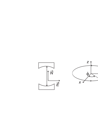
Figure 1: Left: Optical (Fabry-Perot) cavity. The unit vector $\hat{N}$ is parallel to the cavity axis, the unit vector $\hat{E}$ is the polarization of the electromagnetic radiation inside the cavity. Right: Microwave cavity. The ring denotes the electromagnetic cavity mode, parametrized by an angle $0\leq\phi<2\pi$. The polarization $\hat{E}$ is parallel to the $z$ axis, the unit vector $\hat{N}$ is a tangent denoting the direction of the mode for each $\phi$.

II.3 Covalent bonds

The materials quartz (used, for example, in BrilletHall ; HilsHall ) and sapphire (e.g., Braxmaier ; COREs ; MuellerASTROD ) are based on covalent bonds. These bonds have a partial ionic character, i.e., the effective charges of the atoms are $\iota ev$ (as before, $v$ denotes the number of valence charges), where $\iota<1$ can be determined roughly from the difference of the electronegativities of the atoms (see, e.g., Mortimer ). From Eq. (15), we thus obtain length-change coefficients in the per cent range (Table 1). Since the concept of partial ionic character is not an exact concept, these values have limited accuracy. They suggest, however, that the relative length change $\delta L/L$ of a cavity made from quartz or sapphire is negligible compared to the relative change $\delta c/c$ of the speed of light.

Here, we give some arguments indicating that the length change of a covalent crystal may be derived in analogy to ionic crystals. Covalent bonds are given by Coulomb interactions between delocalized electrons, and between the electrons and the atom cores. For our calculation, the main difference to ionic bonds is that the electrons are not localized; instead, they are described by a symmetrized $n$-electron state $\psi^{n}(\vec{x}_{1},\vec{x}_{2},\ldots\vec{x}_{n})$. This state is formed from the single-electron states $\psi_{i}$ as the Slater determinant $(1/\sqrt{N!})\,$Det$(\psi_{i}(\vec{x}_{j}))$. The covalent potential $V_{C}=V_{EC}+V_{EE}+V_{CC}$ is then the sum of the core-core interactions $V_{CC}$

$$V_{CC}=\sum_{a}\sum_{b}\Phi^{(ab)}(\vec{x}_{a}-\vec{x}_{b})$$ (19)

[where $a$ and $b$ enumerate the cores, and $\Phi^{(ab)}(\vec{x}_{a}-\vec{x}_{b})$ is the Coulomb potential between the cores $a$ and $b$ at the locations $\vec{x}_{a}$ and $\vec{x}_{b}$], the electron-core interactions

$$V_{EC}=\sum_{i}\sum_{a}\int(\psi^{n})^{*}\Phi^{(ia)}(\vec{x}_{i}-\vec{x}_{a})\psi^{n}d^{3}x_{1}\ldots d^{3}x_{n}$$ (20)

(where $i$ numerates the electrons and $\Phi^{(ia)}$ is the Coulomb potential between the core $a$ and the electron $i$) and the electron-electron interactions

$$V_{EE}=\sum_{i}\sum_{j}\int(\psi^{n})^{*}\Phi^{(ij)}(\vec{x}_{i}-\vec{x}_{j})\psi^{n}d^{3}x_{1}\ldots d^{3}x_{n}$$ (21)

with $\Phi^{(ij)}$, the Coulomb potential between the electrons $i$ and $j$. Since $\psi^{n}$ is symmetrized, these expressions contain all the terms usually found in the treatment of covalent systems, like the hydrogen molecule. Although the electron wave-functions are spread over the whole crystal volume, their centers of mass are localized at some point within a distance $\bar{a}$ from the cores, where $\bar{a}$ is of atomic dimensions kohn , smaller than the typical distance of atoms in a lattice. As a toy model, we thus assume centers of charge at points $\vec{x}_{\bar{a}}$ at some distance $\bar{a}$ from the locations of the nearest cores. Coulomb forces between these centers of charge and the cores make up an important part of the covalent binding force. The model reduces $V_{EC}$ and $V_{EE}$ to a sum over Coulomb interactions, i.e., we have

$$V_{EC} \sim \sum_{a}\sum_{\bar{a}}\Phi^{(\bar{a}a)}(\vec{x}_{\bar{a}}-\vec{x}_{a})$$ (22)

$$V_{EE} \sim \sum_{\bar{a}}\sum_{\bar{b}}\Phi^{(\bar{a}\bar{b})}(\vec{x}_{\bar{a}}-\vec{x}_{\bar{b}})\,.$$ (23)

The distance $\bar{a}$ between the centers of mass of the delocalized electrons and the cores gives rise to an effective charge of the cores. A calculation of the Lorentz-violating length change could now start from these sums and proceed as for ionic crystals. While this is a simplified model, it indicates that the effect of a Lorentz violating Coulomb potential for covalent bonds will be in analogy to ionic crystals. Thus, estimates for covalent crystals made above should at least give the correct order of magnitude.

III Conclusion and Summary

Table 1: Length change coefficients. The first part of the table contains cubical two-atom crystals, for which the calculation was performed. The length-change coefficients $A$, $a_{\|}$, and $a_{\perp}$ are obtained from Eqs. (14) and (15). The second part contains crystals of other structure with non ionic bindings. Quartz and sapphire have two lattice constants; the axis of highest symmetry is given.

Material	$E_{\rm Y}$	$\rho$	$M$	$\iota^{2}v_{1}v_{2}$	$a$	$A$	$a_{\|}$	$a_{\perp}$
	(GPa)	$\left(\frac{\mbox{g}}{\mbox{cm}^{3}}\right)$			(Å)
NaCl	40	2.1	58	0.64	2.841	-0.14	-0.28	0.10
LiF	64.8	2.64	26	1	2.015	-0.54	-1.06	0.37
NaF	64.8	2.73	32	1	2.135	-0.43	-0.83	0.29
sapphire	497	4.0	102	$1.5$	$13.0$	-0.02	-0.03	0.01
quartz	107	2.2	60	$0.72$	5.4	-0.06	-0.11	0.04

The contributions from Eq. (1) and Eq. (II.2) give

$$\frac{\delta\nu}{\nu} = -a_{\|}\hat{N}(\kappa_{DE})_{\rm lab}\hat{N}$$

$$-\left(\frac{1}{2}+a_{\perp}\right)\left[\hat{E}^{*}(\kappa_{DE})_{\rm lab}\hat{E}\right.$$

$$+\left.(\hat{N}\times\hat{E}^{*})(\kappa_{DE})_{\rm lab}(\hat{N}\times\hat{E})\right]\,.$$

This has been simplified by noting that astrophysical tests lead to $(\kappa_{HB})=-(\kappa_{DE})$ with an accuracy many orders of magnitude higher than attainable in cavity experiments Kostelecky2002 . The second part of Eq. (III) is equivalent to the speed of light change Eq. (1) times $1+2a_{\perp}$, $a_{\perp}\sim 0.01\ldots 0.4$ for the materials in table 1. Additionally, the frequency is sensitive to a term proportional to $a_{\|}\sim-0.03\ldots-1$. For both coefficients, the small coefficients in the per-cent range are for covalent materials (quartz and sapphire); although they are based on a simplified model, they should be accurate enough to conclude that the relative length change of a cavity made from quartz or sapphire is negligible against the change of the speed of light. Since present experiments use these materials, it is indeed possible to analyze them as if the cavity length would not be affected by Lorentz violation. This holds for cavities of any structure, including (microwave) cavities using radial or whispering gallery modes. Their length change is given by Eq. (17). However, future experiments using resonators out of ionic materials, as proposed in BraxmaierPRD will be affected more strongly by the Lorentz violating Coulomb forces (see Table 1); here, it is necessary to analyze them using Eq. (III) rather than Eq. (1).

We note that a cavity experiment is mainly sensitive to the parity odd coefficients Kostelecky2002 of the standard model extension, since both the change of the phase velocity of light, Eq. (1), as well as the cavity length change Eq. (II.2) are dominated by these coefficients. Parity even coefficients that are not tightly constrained by astrophysical birefringence measurements Kostelecky2002 enter cavity experiments only suppressed by $\beta_{\rm lab}$, the velocity of the laboratory with respect to the frame in which one defines the parameters $\kappa_{DE}$ and $\kappa_{HB}$. For experiments on Earth and using a sun centered frame, $\beta_{\rm lab}\sim 10^{-4}$.

We have calculated the length change of electromagnetic cavities due to a modified Coulomb potential arising necessarily from a Lorentz violating velocity of light, as it follows from an extension of the standard model. As a first model, we have assumed that the cavity is made of an ionic crystal. We then extended the model to the covalent bonds of practical materials using the approximate concept of partial charges. Taking this into account for the interpretation of cavity tests of Lorentz invariance, we have shown that the length change effect adds to the hypothetical Lorentz-violating signal derived from a change of the speed of light and increases somewhat the sensitivity of experiments. However, for materials used in present experiments, the increase is at the percent level and thus negligible, as all the Lorentz invariance tests are null tests. As a result, the classical interpretation that neglects the length change is justified (this also holds for microwave cavities and for the classic interferometer tests). For future experiments using ionic crystals as a resonator material, however, the effects derived here are larger and must be taken into account.

As an outlook, we note that the properties of matter and thus the dimensions of cavities also depend on Lorentz-violating terms in the fermionic equations of motion, i.e., a modified Dirac equation KosteleckySME ; Laemmerzahl98 . Strong upper limits on some of these terms have been placed by, e.g., comparisons between atomic clocks Kostelecky99 . In this work, we have focused on the purely electromagnetic sector; the effect of the fermionic terms in cavity experiments will be treated elsewhere. It might be possible to access Lorentz violating fermionic terms in cavity experiments due to the length change they cause. One would compare cavities made from different materials, in order to separate the electromagnetic from the fermionic terms.

Appendix: The repulsive force of the ionic bond

Here, we calculate the modification of the repulsive force due to Lorentz violation. It is caused by the modified wave functions of the ions arising from the modified Coulomb potential between the nucleus and the outer electrons. The repulsive force is a short-range force, so it is sufficient to consider next neighbors only.

Since in ionic crystals, the positive ions are usually small compared to the negative ones Mortimer , we assume as a model that the positive ions are pointlike. The repulsive potential

$$\Phi_{BM}(\vec{R})=\mbox{const}|\psi^{(0)}(\vec{R})|^{2}$$ (25)

is then proportional to the probability density of the outer electrons of the negative ions. $\psi^{(0)}(\vec{R})$ is the unperturbed wave function at the location $\vec{R}$ of the positive ion without Lorentz violation (we assume that the ion-ion interaction does not change appreciably the wave function, which should be satisfied to reasonable accuracy in ionic crystals). The wave function $\psi^{(0)}(\vec{R})$ is proportional to $e^{-\zeta|\vec{R}|}$ for large $|\vec{R}|$ with a constant $\zeta\sim 1/a_{0}$ with the Bohr radius $a_{0}$; the potential $\Phi_{BM}$ is thus a Born-Mayer potential $Be^{-2\zeta|\vec{r}|}$ ($B$ as well as $\zeta$ are phenomenological parameters that are determined by fitting the model to the measurements), which is frequently used as a model of the repulsive force Ashcroft . In the case of Lorentz violation, $\psi(\vec{r})=\psi^{(0)}+\psi^{(1)}$ with a correction $\psi^{(1)}$ that is proportional to $\kappa_{DE}$, which will be calculated for hydrogenlike atoms.

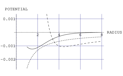
Figure 2: Ion-ion potentials for $n=1,l=0,m=0$ (for other quantum numbers, a similar situation is found). The $x$ axis gives $R$ in units of $a_{0}$, the $y$ axis the potential in arbitrary units. Solid line: $300\delta\Phi_{BM}(\vec{R})$, i.e. the correction to the Born-Mayer Potential, assuming $(\kappa_{DE})^{zz}=1$, enlarged by a factor of 300. Dots: $V(\vec{R})$, i.e. the correction to the Coulomb interaction between two ions for comparison. Dashes: Unperturbed ion-ion Potential $\Phi_{BM}-1/(4\pi|R|)$. The constant const$=15$ has been inserted as to obtain a minimum of the total unperturbed ion-ion potential around $R$=5, as commonly found in ionic crystals (e.g., $R=5.3a_{0}$ for NaCl). The correction to the repulsive potential is negligible compared to the correction of the Coulomb potential.

For this calculation, we denote the unperturbed state of hydrogen $|nlm>^{(0)}$ with a principal quantum number $n$, angular momentum $l$ and magnetic quantum number $m$. The corresponding wave function $\psi_{nlm}^{(0)}(\vec{r})$ can be factorized into a radial function $R_{nl}(r)$ that depends solely on the radius coordinate $r$, and spherical harmonics $Y_{l}^{m}(\theta,\phi)$. Only the ground state $n=1$ is not degenerate; for the $n=2$ states, the use of the perturbation theory of nondegenerate states is still possible since, due to the nature of the matrix elements calculated below, the degenerate $n=2$ states do not mix. For $n=1,2$, the state $|nlm>=|nlm>^{(0)}+|nlm>^{(1)}$ in first order perturbation theory is given by

$$|nlm>^{(1)}={\sum_{n^{\prime}l^{\prime}m^{\prime}}}^{\prime}\frac{<nlm|V|n^{\prime}l^{\prime}m^{\prime}>}{E_{n}-E_{n^{\prime}}}|n^{\prime}l^{\prime}m^{\prime}>$$ (26)

with $V$ given by Eq. (2). Inserted into Eq. (25), this leads to a correction to the Born-Mayer potential

$$\delta\Phi_{BM}(\vec{R})=2\,\mbox{const}{\sum_{n^{\prime}l^{\prime}m^{\prime}}}^{\prime}\frac{<nlm|V|n^{\prime}l^{\prime}m^{\prime}>}{E_{n}-E_{n^{\prime}}}$$ (27)

$$\times|\psi_{nlm}^{(0)}(\vec{R})\psi_{n^{\prime}l^{\prime}m^{\prime}}^{(0)}(\vec{R})|\,.$$

We apply coordinates in which $\kappa_{DE}$ is diagonal with the diagonal elements $\kappa_{xx},\kappa_{yy},$ and $\kappa_{zz}$. Applying polar coordinates with the $\theta=0$ axis parallel to the $z$ axis, the Lorentz violating correction to the Coulomb potential $V$ can be written as

$$V=\frac{e^{2}}{8\pi r}[(\kappa_{xx}\sin^{2}\phi+\kappa_{yy}\cos^{2}\phi)\sin^{2}\theta+\kappa_{zz}\cos^{2}\theta]\,.$$ (28)

Since in first order perturbation theory, the change of the wave function $|nlm>^{(1)}$ for a sum of perturbations $\sum_{i}V_{i}$ is a linear combination of the changes for each single perturbation $V_{i}$, it is sufficient to consider the term proportional to $\kappa_{zz}$. In configuration space,

$$<nlm|r^{-1}\cos^{2}\theta|n^{\prime}l^{\prime}m^{\prime}>=\int R_{nl}(r)\frac{1}{r}R_{n^{\prime}l^{\prime}}(r)r^{2}dr$$

$$\times\int Y_{l}^{m}(\theta,\phi)\cos^{2}\theta Y_{l^{\prime}}^{m^{\prime}}(\theta,\phi)\sin\theta d\theta d\phi\quad$$ (29)

with the normalized radial functions

$$R_{nl}=\frac{2}{n^{2}}\sqrt{\frac{\zeta^{3}(n-l-1)!}{(n+1)!}}\left(2\frac{\zeta r}{n}\right)^{l}e^{-\zeta r/n}L_{n-l-1}^{2l+1}\left(2\frac{\zeta r}{n}\right)$$ (30)

where $L_{p}^{k}(z)$ are associated Laguerre polynomials as defined in Gradstein . For the treatment of hydrogenlike atoms, $\zeta=Z/a_{0}$ is given by the core charge number $Z$. Here, we take $\zeta=1/a_{0}$. Using

$$Y_{l}^{m}(\theta,\phi)=\sqrt{\frac{2l+1}{4\pi}\frac{(l-m)!}{(l+m)!}}P_{l}^{m}(\cos\theta)e^{im\phi}\,,$$ (31)

[where $P_{l}^{m}(x)$ are the associated Legendre functions], it is easy to verify that the $\phi$ integration gives $\pi\delta_{m,m^{\prime}}$. For the $\theta$ integration, we substitute $x=\cos\theta$. Applying the relation Gradstein

$$x(2l+1)P_{l}^{m}(x)=(l-m+1)P_{l+1}^{m}(x)+(l+m)P_{l-1}^{m}(x)$$ (32)

two times and using the normalization

$$\int_{-1}^{1}P_{l}^{m}(x)P_{l^{\prime}}^{m}(x)dx=\frac{2}{2l+1}\frac{(l+m)!}{(l-m)!}\delta_{ll^{\prime}}\,,$$ (33)

it can be shown that

$$\int_{-1}^{1}P_{l}^{m}(x)P_{l^{\prime}}^{m}(x)x^{2}dx$$

$$=\left\{\begin{array}[]{lr}\frac{4l^{2}-1+(l+m)(4l^{2}+4m-3)}{(2l-1)(2l+1)^{2}(2l+3)}\frac{2(l+m)!}{(l-m)!}\,,&l^{\prime}=l\\ &\\ \frac{2}{(2l^{\prime}-1)(2l^{\prime}+1)(2l^{\prime}+3)}\frac{(l+m+1\pm 1)!}{(l-m-1\pm 1)!}\,,&l^{\prime}=l\pm 2\end{array}\right.$$ (37)

and zero otherwise. That means, the matrix element is nonzero only for $l=l^{\prime}$ or $l=l^{\prime}\pm 2$. However, for $l=l^{\prime}$, the radial integral is nonzero only for $n=n^{\prime}$; that term is not needed for this calculation. Combining these results leads to the more simple expression for the correction of the Born-Mayer potential

$$\delta\Phi_{BM}(\vec{R}) = 2\,\mbox{const}\sum_{n^{\prime}=3}^{\infty}\frac{<nlm|V|n^{\prime}l+2m>}{E_{n}-E_{n^{\prime}}}$$ (38)

$$\times|\psi_{nlm}^{(0)}(\vec{R})\psi_{n^{\prime}\,l+2\,m}^{(0)}(\vec{R})|$$

(for $n=1,2$, $0\leq l<n$, and $|m|\leq l$). Formally, the series should be summed up to infinity. However, the terms decay rapidly with increasing $n^{\prime}$. The correction of the Born-Mayer potential due to Lorentz violation can thus be obtained and compared to the correction of the Coulomb potential due to the same Lorentz violation (Fig. 2). Here, $\vec{R}$ was assumed parallel to the $z$ direction. If $\vec{R}$ is not perpendicular to the $z$ direction, the correction to the Born-Mayer potential is smaller. From this calculation, it can be concluded that the Lorentz-violating modification of the repulsive potential $\delta\Phi_{BM}$ is negligible compared to the modification of the Coulomb potential, at least for the $n=1$ and 2 states that have been considered in this simple model. This is due to the small magnitude of the matrix elements $<nlm|V|n^{\prime}l^{\prime}m^{\prime}>$, which are also small for high $n$ and $n^{\prime}$ (they even decrease with increasing $n$ and $n^{\prime}$). So, although for $n\geq 3$, the perturbation theory for degenerate states should be applied, this will not dramatically change the magnitude of $\delta\Phi_{BM}$ and thus our conclusion that $\delta\Phi_{BM}$ is negligible remains valid.

References

- (1) A.A. Michelson, Am. J. Sci. 22, 120 (1881); A.A. Michelson and E.W. Morley, ibid. 34, 333 (1887); Phil. Mag. 24, 449 (1897).
- (2) R.J. Kennedy and E.M. Thorndike, Phys. Rev. 42, 400 (1932).
- (3) A. Brillet and J.L. Hall, Phys. Rev. Lett. 42, 549 (1979).
- (4) D. Hils and J.L. Hall, Phys. Rev. Lett. 64, 1697 (1990).
- (5) S. Buchman et al., Adv. Space Res. 25, 1251 (2000).
- (6) C. Lämmerzahl et al., Class. Quantum Grav. 18, 2499 (2001).
- (7) C. Braxmaier et al., Phys. Rev. Lett. 88, 010401 (2001).
- (8) H. Müller et al., Int. J. Mod. Phys. D 11, 1101 (2002).
- (9) P. Wolf et al., Phys. Rev. Lett. 90, 060402 (2003); J.A. Lipa et al., ibid. 90, 060403 (2003).
- (10) V.A. Kostelecký and S. Samuel, Phys. Rev. D 39, 683 (1989).
- (11) J. Ellis et al, Gen. Relativ. Gravit. 32, 1777 (2000); gr-qc/9909085; Gen. Relativ. Gravit. 31, 1257 (1999).
- (12) R. Gambini and J. Pullin, Phys. Rev. D 59, 124021 (1999).
- (13) J. Alfaro, H.A. Morales-Técotl, and L.F. Urrutia, Phys. Rev. D 65, 103509 (2002); Phys. Rev. Lett. 84, 2318 (2000).
- (14) D. Colladay and V.A. Kostelecký, Phys. Rev. D 55, 6760 (1997); 58, 116002 (1998); R. Bluhm et al., Phys. Rev. Lett. 88, 090801 (2002) and references cited therein.
- (15) V.A. Kostelecky and M. Mewes, Phys. Rev. D 66, 056005 (2002).
- (16) H.P. Robertson, Rev. Mod. Phys 21, 378 (1949).
- (17) R.M. Mansouri and R.U. Sexl, Gen. Relativ. Gravit. 8, 497 (1977); 8, 515 (1977); 8, 809 (1977)
- (18) C. Lämmerzahl et al., Int. J. Mod. Phys. D, 11 1109 (2002).
- (19) C.M. Will, Theory and Experiment in Gravitational Physics, revised ed. (Cambridge University Press, Cambridge, England, 1993).
- (20) Other parameters are strongly bounded by astrophysical polarization measurements. We assume here.
- (21) Lorentz violation might also influence the boundary conditions for the electromagnetic fields inside the cavity, adding a phase shift to radiation reflected at the boundary. This results in a frequency shift ( is the wavelength inside the cavity), which would have to be added to (1). However, it is negligible, at least in optical cavities, where is of order .
- (22) C.M. Will, Phys. Rev. D 45, 403 (1992).
- (23) C. Lämmerzahl and M.P. Haugan, Phys. Lett. A 282, 223 (2001).
- (24) E.W. Morley and D.C. Miller, Philos. Mag. 8, 753 (1904); 9, 680 (1905)
- (25) G. Woan, The Cambridge Handbook of Physics Formulas (Cambridge University Press, Cambridge, England, 2000), p. 80.
- (26) C. Braxmaier et al., Phys. Rev. D 64, 042001 (2001).
- (27) N.W. Ashcroft, N.D. Mermin, Solid state physics, International ed. (Saunders College, Fort Worth, 1976)
- (28) S. Seel et al., Phys. Rev. Lett 78, 4741 (1997); R. Storz et al., Opt. Lett. 23, 1031 (1998).
- (29) C.E. Mortimer, Chemistry (Wadsworth, Belmont, Ca. 1986).
- (30) W. Kohn, Phys. Rev. 133, A171 (1964).
- (31) C. Lämmerzahl, Class. Quantum Grav. 14, 13 (1998).
- (32) V.A. Kostelecky and C.D. Lane, Phys. Rev. D 60, 116010 (1999); R. Bluhm et al., Phys. Rev. Lett. 88, 090801 (2002) and references cited therein.
- (33) I.S. Gradsteyn and I.M. Ryzhik, Table of Integrals, Series, and Products, sixth ed. (Academic, San Diego, 2000).