SLAC-PUB-9614 December 2002

Brane-localized Kinetic Terms in the Randall-Sundrum Model

H. Davoudiasl^1,a, J.L. Hewett^2,b, and T.G. Rizzo^2,c

¹School of Natural Sciences, Institute for Advanced Study, Princeton, NJ 08540

²Stanford Linear Accelerator Center, Stanford, CA, 94309

We examine the effects of boundary kinetic terms in the Randall-Sundrum model with gauge fields in the bulk. We derive the resulting gauge Kaluza-Klein (KK) state wavefunctions and their corresponding masses, as well as the KK gauge field couplings to boundary fermions, and find that they are modified in the presence of the boundary terms. In particular, for natural choices of the parameters, these fermionic couplings can be substantially suppressed compared to those in the conventional Randall-Sundrum scenario. This results in a significant relaxation of the bound on the lightest gauge KK mass obtained from precision electroweak data; we demonstrate that this bound can be as low as a few hundred GeV. Due to the relationship between the lightest gauge KK state and the electroweak scale in this model, this weakened constraint allows for the electroweak scale to be near a TeV in this minimal extension of the Randall-Sundrum model with bulk gauge fields, as opposed to the conventional scenario.

1 Introduction

The Randall-Sundrum (RS) model [1] offers a new approach to the hierarchy problem. Within this scenario, the disparity between the electroweak and Planck scales is generated by the curvature of a 5-dimensional (5-d) background geometry which is a slice of anti-de Sitter ($AdS_{5}$) spacetime. This slice is bounded by two 3-branes of equal and opposite tensions sitting at the fixed points of an $S^{1}/Z_{2}$ orbifold which are located at $\phi=0,\pi$ where $\phi$ is the coordinate of the $5^{th}$ dimension. The 5-d warped geometry then induces an effective 4-d scale $\Lambda_{\pi}$ of order a TeV on the brane at $\phi=\pi$, the so-called TeV brane. $\Lambda_{\pi}$ is exponentially smaller than the effective scale of gravity given by the reduced Planck scale, $\overline{M}_{Pl}$, with the suppression being determined by the product of the 5-d curvature parameter $k$ and the separation $r_{c}$ of the two branes, i.e., $\Lambda_{\pi}=\overline{M}_{Pl}e^{-kr_{c}\pi}$. In this theory, the original parameters of the 5-d action are all naturally of the size $\sim\overline{M}_{Pl}$, while in the 4-d picture a hierarchy with $\Lambda_{\pi}/\overline{M}_{Pl}\,\,\hbox to0.0pt{\raise 3.0pt\hbox{$<$}\hss}{\lower 3.0pt\hbox{$\sim$}}\,\,10^{-15}$ appears. It has been demonstrated [2] that this scenario is naturally stabilized without the introduction of fine-tuning for $kr_{c}\simeq 11$, which is the numerical value required to generate the hierarchy. This model leads to a distinct set of phenomenological signatures that may soon be revealed by experiments at the TeV scale; these have been examined in much detail [3, 4, 5].

For model building purposes, it is advantageous to extend the original framework of the RS model, where gravity alone propagates in the extra dimension, to the case where at least some of the Standard Model (SM) fields are present in the bulk [6]. The simplest such possibility is to have the SM gauge fields in the bulk [4, 5], while the other SM fields remain localized on the TeV brane. This scenario was examined in detail some time ago [4] where it was found that the couplings of the Kaluza-Klein (KK) excitations of the bulk gauge fields to matter on the boundary were enhanced by a factor of $\sqrt{2\pi kr_{c}}$ compared to those of the corresponding zero-mode states. Since $kr_{c}\simeq 11$ as discussed above, this enhancement is numerically significant and is approximately a factor of $\simeq 8.4$. Severe constraints are then imposed on the gauge KK excitations from precision electroweak measurements; these imply that the mass of the lightest gauge KK state must be heavy with $m_{1}\geq 25-30$ TeV. Due to the relation in this model between the masses of the KK states and the scale of physics on the TeV brane, this bound then correspondingly requires that $\Lambda_{\pi}\geq 100$ TeV. This places such a scenario in a very unfavorable light in terms of its original motivation of resolving the hierarchy.

Here, we investigate whether Brane Localized Kinetic Terms (BLKT’s) for bulk gauge fields can modify these results. Recently, Carena, Tait and Wagner [7] examined the phenomenological influence of such localized kinetic terms for bulk gauge fields within the context of flat TeV^-1-sized extra dimensions. These authors showed that such terms can lead to significant modifications to the gauge KK spectrum, as well as to the KK state self-couplings and couplings to fields remaining on orbifold fixed points. Localized kinetic terms are expected to be present on rather general grounds in any orbifolded theory, as was shown by Georgi, Grant and Hailu [8], since they are needed to provide counterterms for divergences that are generated at one loop. In addition, these boundary terms can have important implications in a number of different situations such as model building [9], the construction of GUTs in higher dimensions with flat [10] or warped [11] geometries, and, in a different context, the quasilocalization of gravity [12]. Up to now the phenomenological implications of BLKT’s in the case of warped extra dimensions have not been examined.

We examine the effects of localized kinetic terms in the case where the SM gauge fields are present in the RS bulk and the remaining SM fields are on the TeV-brane. As in the case of TeV^-1-sized extra dimensions, we find that these boundary terms alter both the KK spectrum as well as their associated couplings to the remaining wall fields, but in a manner which is quite distinctive due to the curved geometry in this scenario. We will show that for a reasonable range of model parameters these modifications can be quite significant and lead to a natural reduction in the strength of the KK couplings. This allows the restrictions on $\Lambda_{\pi}$ to be reduced by more than an order of magnitude and it would then no longer be unfavorable to have gauge fields be the only SM fields present in the RS bulk. The next section contains a detailed discussion of the modification of the usual gauge boson analysis within the RS framework due to the existence of brane localized kinetic terms. In Section 3 we discuss the implication of these results for the phenomenology of this scenario and our conclusions can be found in Section 4. Special limits of the KK mass equation are discussed in an Appendix.

2 Formalism

In this section, we derive the wavefunctions and the KK mass eigenvalue equation for bulk gauge fields with BLKT’s in the RS scenario. We then compute the coupling of the gauge field KK modes to 4-d fermions localized on the TeV brane, where the scale of physics is of order the electroweak scale. Our derivation will demonstrate how the boundary terms modify these couplings from their original form and result in a possible softening of the precision electroweak bounds on the mass of the lightest KK gauge state. In the rest of the paper, KK modes refer to those from the bulk gauge fields, unless otherwise specified.

We perform our calculations for a $U(1)$ gauge field; the generalization to the case of non-Abelian fields is straightforward. Let us start with the 5-d action for the gauge sector

$$S_{A}= - \frac{1}{4}\int d^{5}x\,\sqrt{-G}\,\left\{G^{AM}G^{BN}F_{AB}F_{MN}\right.$$ (1)

$$+ \left.[c_{0}\,\delta(\phi)+c_{\pi}\,\delta(\phi-\pi)]\,G^{\alpha\mu}G^{\beta\nu}F_{\alpha\beta}F_{\mu\nu}\right\}\,,$$

where the terms proportional to $c_{0}$ and $c_{\pi}$ represent the kinetic terms for the branes located at $\phi=0,\,\pi$, respectively, and the metric $G_{MN}$ is given by the RS line element

$$ds^{2}=e^{-2\sigma}\eta_{\mu\nu}dx^{\mu}dx^{\nu}-r_{c}^{2}d\phi^{2}\,\,\,\,;\,\,\,\,\sigma=kr_{c}|\phi|\,.$$ (2)

Here the dimensionless constants $c_{0,\pi}$ would naturally be expected to be of order unity. Note that we can neglect terms proportional to $\partial_{5}A_{\mu}$ on either brane as demonstrated by [7]. We will work in the $A_{5}=0$ gauge so that terms including $A_{5}$ can also be neglected. Thus only the usual 4-d kinetic term appears in the brane contributions to the action. In our notation, $A,B,\ldots=0,\ldots,3,5$ and $\alpha,\beta,\ldots=0,\ldots,3$. Here, $k$ is the 5-d curvature scale, $r_{c}$ is the compactification radius, and $x^{5}=r_{c}\phi$ with $-\pi\leq\phi\leq\pi$. The field strength is given by

$$F_{MN}=\partial_{M}A_{N}-\partial_{N}A_{M}\,.$$ (3)

The gauge field is assumed to have the KK expansion

$$A_{\mu}(x,\phi)=\sum_{n}A_{\mu}^{(n)}(x)\frac{\chi^{(n)}(\phi)}{\sqrt{r_{c}}}\,.$$ (4)

Substituting the above expansion in the action (1) yields

$$S_{A}= - \frac{1}{4r_{c}}\int d^{5}x\sum_{m,n}\,\left\{[1+c_{0}\,\delta(\phi)+c_{\pi}\,\delta(\phi-\pi)]\,F^{\mu\nu(m)}F_{\mu\nu}^{(n)}\chi^{(m)}\chi^{(n)}\right.$$ (5)

$$- \left.(2/r_{c}^{2})\,A^{\mu(m)}A_{\mu}^{(n)}e^{-2\sigma}[(d/d\phi)\chi^{(m)}][(d/d\phi)\chi^{(n)}]\right\}\,,$$

where now all the Lorentz indices are contracted using the 4-d Minkowski metric. In order to cast this action in the diagonal form, we demand

$$\int d\phi\,[1+c_{0}\,\delta(\phi)+c_{\pi}\,\delta(\phi-\pi)]\,\chi^{(m)}\chi^{(n)}=Z_{n}\delta^{mn}$$ (6)

and

$$\frac{1}{r_{c}^{2}}\int d\phi\,e^{-2\sigma}\Big{[}\frac{d}{d\phi}\chi^{(m)}\Big{]}\Big{[}\frac{d}{d\phi}\chi^{(n)}\Big{]}=Z_{n}m_{n}^{2}\,\delta^{mn}\,.$$ (7)

These equations imply

$$\frac{d}{d\phi}\left(e^{-2\sigma}\frac{d}{d\phi}\chi^{(n)}\right)+[1+c_{0}\,\delta(\phi)+c_{\pi}\,\delta(\phi-\pi)]\,r_{c}^{2}\,m_{n}^{2}\,\chi^{(n)}=0\,.$$ (8)

Away from the boundaries at $\phi=0,\pi$, the solution to Eq.(8) is given by [4, 5]

$$\chi^{(n)}(\phi)=\frac{e^{\sigma}}{N_{n}}\,\zeta_{1}(z_{n})\,,$$ (9)

where $z_{n}(\phi)\equiv(m_{n}/k)e^{\sigma}$; $\zeta_{q}(z_{n})\equiv[J_{q}(z_{n})+\alpha_{n}\,Y_{q}(z_{n})]$, with $J_{q}$ and $Y_{q}$ denoting the usual Bessel functions of order $q$. The normalization $N_{n}$ is set by the condition

$$\int_{-\pi}^{+\pi}d\phi~{}[\chi^{(n)}]^{2}=1\,,$$ (10)

implying that the zero mode is given by $\chi^{(0)}=1/\sqrt{2\pi}$. Integrating Eq.(8) around the fixed points $\phi=0$ and $\phi=\pm\pi$ yields

$$2\frac{d}{d\phi}\chi^{(n)}(0)+c_{0}\,r_{c}^{2}m_{n}^{2}\,\chi^{(n)}(0)=0$$ (11)

and

$$2\frac{d}{d\phi}\chi^{(n)}(\pi)-e^{2kr_{c}\pi}c_{\pi}r_{c}^{2}\,m_{n}^{2}\,\chi^{(n)}(\pi)=0\,,$$ (12)

respectively.

Let $\varepsilon_{n}\equiv z_{n}(0)$. For light KK modes with masses $m_{n}\sim 1$ TeV, which are of phenomenological interest, $\varepsilon_{n}\ll 1$; for $k\sim\overline{M}_{Pl}$ we have $\varepsilon_{n}\sim 10^{-15}$. Substituting for $\chi^{(n)}$ from Eq.(9) in Eq.(11), and using the identity

$$x\zeta_{0}(x)=\zeta_{1}(x)+x\zeta_{1}^{\prime}(x)\,,$$ (13)

we obtain

$$\alpha_{n}=-\frac{J_{0}(\varepsilon_{n})+\delta_{0}\varepsilon_{n}J_{1}(\varepsilon_{n})}{Y_{0}(\varepsilon_{n})+\delta_{0}\varepsilon_{n}Y_{1}(\varepsilon_{n})}\,,$$ (14)

where $\delta_{0}\equiv c_{0}k\,r_{c}/2$ and a prime $(^{\prime})$ denotes a derivative. Note that with $c_{0}$ of order unity, we may expect values of $\delta_{0}$ of order 10 since $kr_{c}$ takes on the value $\sim 11$ in order to address the hierarchy. Similarly, from Eq.(12), we obtain

$$\zeta_{0}(x_{n})-\delta_{\pi}x_{n}\zeta_{1}(x_{n})=0\,,$$ (15)

where $\delta_{\pi}\equiv c_{\pi}k\,r_{c}/2$ and $x_{n}\equiv z_{n}(\pi)$. The roots $x_{n}$ of Eq.(15) yield the gauge KK mass spectrum, $m_{n}=x_{n}ke^{-kr_{c}\pi}$. We will study various limits of this root equation in the Appendix. Following the same arguments as above, we may expect that $|\delta_{0,\pi}|\,\,\hbox to0.0pt{\raise 3.0pt\hbox{$<$}\hss}{\lower 3.0pt\hbox{$\sim$}}\,\,{\cal O}(10)$, assuming no fine-tuning.

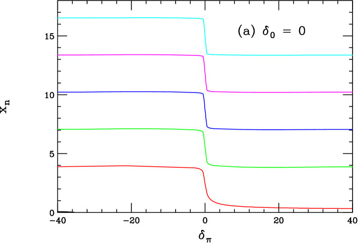
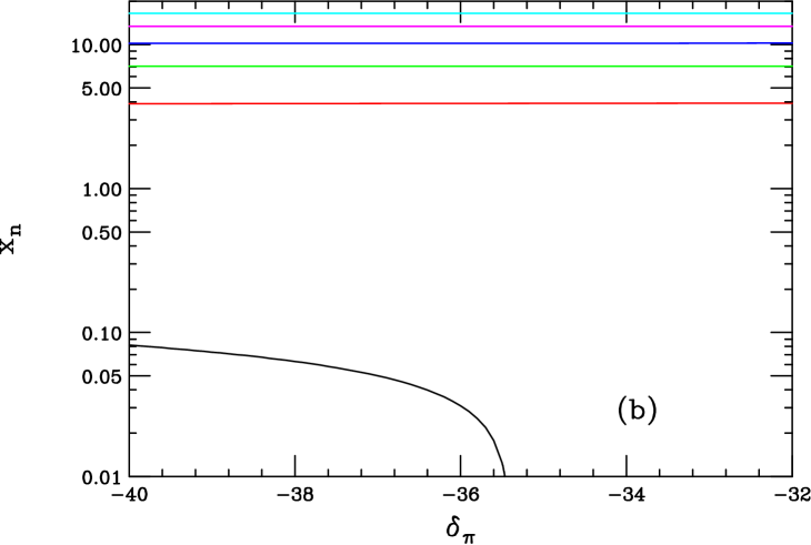
Figure 1: (a) The behavior of the first five roots as $\delta_{\pi}$ is varied, assuming $\delta_{0}=0$. Note the sharp increase in $x_{n}$ near $\delta_{\pi}=0$ for all KK levels. (b) The large negative $\delta_{\pi}$ region is expanded to show the new root originating at the value $\delta_{\pi}=-kr_{c}\pi\simeq-35.4$.

Due to the exponentially small value of $\epsilon_{n}$, it may first appear that the $\delta_{0}$-dependent corrections to $\alpha_{n}$ are highly suppressed, and that $\alpha_{n}$ is small, of order $\sim 0.01$, as in the standard RS scenario. However, an expansion of Eq. (14) in the parameter $\varepsilon_{n}$ yields

$$\alpha_{n}\simeq-\frac{\pi/2}{\ln(x_{n}/2)-k\,r_{c}\,\pi+\gamma-\delta_{0}}\,,$$ (16)

where $\gamma\approx 0.577$ is Euler’s constant. $\alpha_{n}$ remains small over most regions of parameter space of interest here, except for when $\delta_{0}\simeq-kr_{c}\pi\simeq-35.4$. There are two sources of modifications to $\alpha_{n}$ as compared to the original RS framework due to the presence of the boundary terms: (1) the appearance of the term proportional to $\delta_{0}$ in the denominator which is not suppressed by the exponential warp factor, and (2) the BLKT-modified values of $x_{n}$. In our numerical analyses we will use the exact expression for $\alpha_{n}$, rather than the approximate version given above, and we take $kr_{c}=11.27$.

To get a flavor of how the KK tower mass spectrum is modified in this scenario with BLKT’s, we must solve Eq.(15) for a range of values of $\delta_{0,\pi}$. We first take the simplest possibility by setting $\delta_{0}=0$, and examine the roots $x_{n}$ as a function of $\delta_{\pi}$. Our results are displayed in Fig. 1. From Fig. 1a, we see that in the region near $\delta_{\pi}=0$ the roots undergo a substantial shift but remain relatively independent of variations in $\delta_{\pi}$ away from the origin. For large negative values of $\delta_{\pi}$, the roots are almost the same as those obtained in the case of the graviton KK spectrum in the original RS framework [3]. This can be seen analytically by taking the limit of large $|\delta_{\pi}|$ in Eq.(15) and neglecting $\alpha_{n}\ll 1$. When the value of $-\delta_{\pi}$ exceeds $kr_{c}\pi$, a new root appears which is barely perceptible in Fig. 1a, but whose turn-on is shown in detail in Fig. 1b. The analytical source of this root is discussed in the Appendix. We will later see that this signals the appearance of an unphysical ghost, i.e., a tachyonic state with negative norm.

When $\delta_{0}\neq 0$ the modifications to the roots are sensitive to the sign of $\delta_{0}$. For $\delta_{0}=\delta_{\pi}$, and in the range $\delta_{\pi}\mathrel{\mathchoice{\lower 3.01385pt\vbox{\halign{$\matth\displaystyle\hfil#\hfil$\cr>\crcr\sim\crcr}}}{\lower 3.01385pt\vbox{\halign{$\matth\textstyle\hfil#\hfil$\cr>\crcr\sim\crcr}}}{\lower 3.01385pt\vbox{\halign{$\matth\scriptstyle\hfil#\hfil$\cr>\crcr\sim\crcr}}}{\lower 3.01385pt\vbox{\halign{$\matth\scriptscriptstyle\hfil#\hfil$\cr>\crcr\sim\crcr}}}}-30$, the roots appear to be very similar to those obtained when $\delta_{0}=0$, as is shown in Fig. 2a. The major difference in this case is the location of where the additional ghost root materializes; as shown in the Appendix, this root appears at the value $\delta_{\pi}=-(kr_{c}\pi+\delta_{0})$. When $\delta_{0}>(<)0$ the turn-on of this root thus moves to smaller (larger) values of $\delta_{\pi}$. In the case $\delta_{0}=\delta_{\pi}$, Fig. 2a shows that the new root appears at $\delta_{\pi}=-kr_{c}\pi/2$ as expected. We also see that for $\delta_{\pi}\,\,\hbox to0.0pt{\raise 3.0pt\hbox{$<$}\hss}{\lower 3.0pt\hbox{$\sim$}}\,\,-\pi kr_{c}$ the roots approach those which govern the KK graviton spectrum, as discussed above. In Fig. 2b, we display the roots for the case $\delta_{0}=-\delta_{\pi}$. For most values of $\delta_{\pi}$ shown in the figure, these are found to be similar to the case where $\delta_{0}=0$ except that a new light root does not appear in this case. This is as expected, based on the discussion in the Appendix. When $\delta_{\pi}$ is large and positive, $\delta_{\pi}\mathrel{\mathchoice{\lower 3.01385pt\vbox{\halign{$\matth\displaystyle\hfil#\hfil$\cr>\crcr\sim\crcr}}}{\lower 3.01385pt\vbox{\halign{$\matth\textstyle\hfil#\hfil$\cr>\crcr\sim\crcr}}}{\lower 3.01385pt\vbox{\halign{$\matth\scriptstyle\hfil#\hfil$\cr>\crcr\sim\crcr}}}{\lower 3.01385pt\vbox{\halign{$\matth\scriptscriptstyle\hfil#\hfil$\cr>\crcr\sim\crcr}}}}\pi kr_{c}$, the roots again approach those for the case of KK gravitons, as anticipated.

When $\delta_{\pi}=0$, the roots exhibit a weak dependence on $\delta_{0}$ away from the $\delta_{0}=-kr_{c}\pi$ region; this can be seen in Fig. 3. The $\delta_{0}$ dependence of the roots is isolated in the coefficients $\alpha_{n}$ as seen in Eq.(16). From this we see that the roots have a slightly negative slope with increasing $\delta_{0}$.

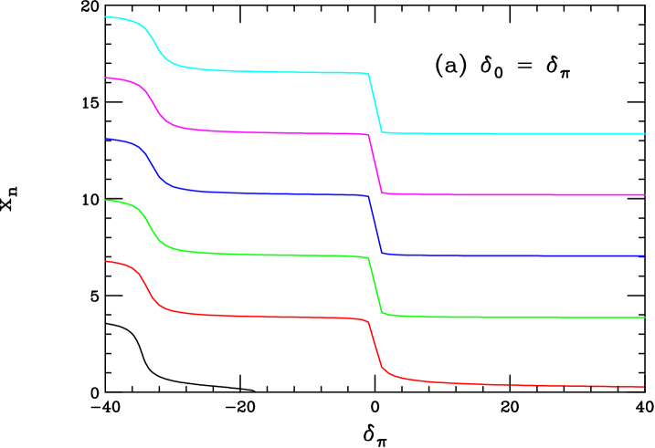
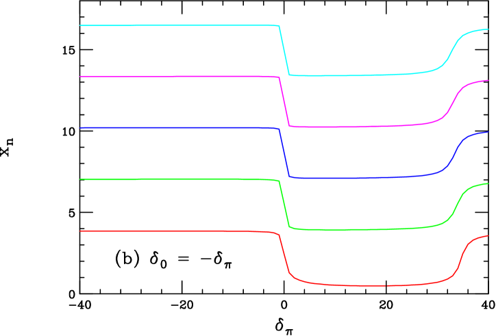
Figure 2: (a) The behavior of the first five roots as a function of $\delta_{\pi}$ for the case $\delta_{0}=\delta_{\pi}$. Here, the new root appears at the value $\delta_{\pi}=-kr_{c}\pi/2\simeq-17.7$. (b) Same as above for the case $\delta_{0}=-\delta_{\pi}$.

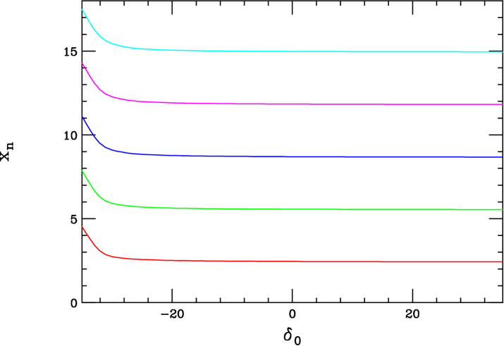
Figure 3: The behavior of the first five roots as a function of $\delta_{0}$ taking $\delta_{\pi}=0$.

3 Analysis

In this section, we study the couplings of the KK modes to the boundary fermions at $\phi=\pi$. The values of these couplings are the driving force behind the important constraints on the mass of the lightest KK gauge field in the original RS scenario [4]. In this section, we reexamine these bounds in the presence of brane localized kinetic terms. To begin, we note that the diagonalization conditions (6) and (7) yield the 4-d action

$$S_{A}=-\frac{1}{4}\int d^{4}x\sum_{n}\,Z_{n}\left(F^{\mu\nu(n)}F_{\mu\nu}^{(n)}-2m_{n}^{2}A^{\mu(n)}A_{\mu}^{(n)}\right)\,,$$ (17)

where we have

$$Z_{n}=1+c_{0}[\chi^{(n)}(0)]^{2}+c_{\pi}[\chi^{(n)}(\pi)]^{2}\,.$$ (18)

Note that for physical fields, we demand that $Z_{n}>0$ for all $n\geq 0$.

The coupling of a bulk gauge field $A_{\mu}$ to fermions $\psi$ localized at $\phi=\pi$ is given by the action

$$S_{\psi}=-\int d\phi\,d^{4}x\,(detV)\,g_{5}\,\bar{\psi}V^{\mu}_{\alpha}\gamma^{\alpha}A_{\mu}(x,\phi)\psi\,\delta(\phi-\pi)\,,$$ (19)

where $V^{\mu}_{\alpha}=e^{\sigma}\eta^{\mu}_{\alpha}$ is the vielbein, $detV=e^{-4\sigma}$, and $g_{5}$ is the 5-d coupling constant. Using the expansion (4) in Eq.(19), we obtain

$$S_{\psi}=-\int d^{4}x\left[\frac{g_{5}}{\sqrt{2\pi r_{c}}}\,\bar{\psi}\gamma^{\mu}A_{\mu}^{(0)}\psi+\sum_{n\neq 0}g_{5}{e^{\pi kr_{c}}\zeta_{1}(x_{n})\over N_{n}\sqrt{r_{c}}}\,\bar{\psi}\gamma^{\mu}A_{\mu}^{(n)}\psi\right]\,,$$ (20)

where we have performed the redefinition $\psi\rightarrow e^{3kr_{c}\pi/2}\psi$ to make the $\psi$ kinetic terms canonical. Here, we have used the normalization

$$N_{n}^{2}={x_{n}^{2}\over kr_{c}\epsilon_{n}^{2}}\,\zeta_{1}^{2}(x_{n})W\,,$$ (21)

where

$$W=(1-2\delta_{\pi}+\delta_{\pi}^{2}x_{n}^{2})\left[1-{\epsilon_{n}^{2}\zeta_{1}^{2}(\epsilon_{n})[1+2\delta_{0}+\epsilon_{n}^{2}\delta_{0}^{2}]\over x_{n}^{2}\zeta_{1}^{2}(x_{n})[1-2\delta_{\pi}+x_{n}^{2}\delta_{\pi}^{2}]}\right]\,.$$ (22)

Note that this normalization is mode dependent. To bring the gauge field kinetic terms in Eq.(17) into the canonical form, we require

$$A^{(n)}_{\mu}\rightarrow\frac{A^{(n)}_{\mu}}{\sqrt{Z_{n}}}\,.$$ (23)

Eqs.(20) and (23) then yield

$$S_{\psi}=-\int d^{4}x\left[g_{0}\,\bar{\psi}\gamma^{\mu}A_{\mu}^{(0)}\psi+\sum_{n\neq 0}g_{n}\bar{\psi}\gamma^{\mu}A_{\mu}^{(n)}\psi\right]\,,$$ (24)

with

$$g_{0}\equiv{g_{5}\over\sqrt{2\pi r_{c}Z_{0}}}$$ (25)

and

$$g_{n}\equiv g_{0}\sqrt{2\pi kr_{c}}\sqrt{{Z_{0}\over WZ_{n}}}\,.$$ (26)

Here, $g_{0}$ is identified as the usual 4-d coupling constant for the interactions of the fermions with the zero-mode KK state. The KK excitation couplings are given by $g_{n}$, which due to the presence of the boundary terms are now mode dependent. Without the presence of the brane kinetic terms, one obtains $Z_{0}=Z_{n}=1$ which yields the result that $g_{n}$ is an approximately mode-independent constant given by $g_{n}\simeq g_{0}\sqrt{2\pi kr_{c}}$, since in this case $\alpha_{n}\sim 10^{-2}$ and $W\simeq 1$.

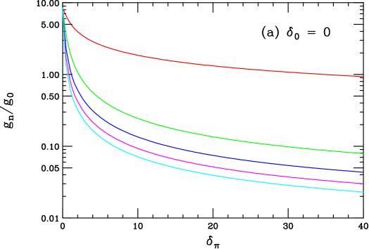
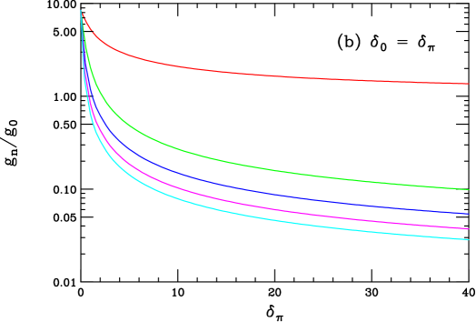
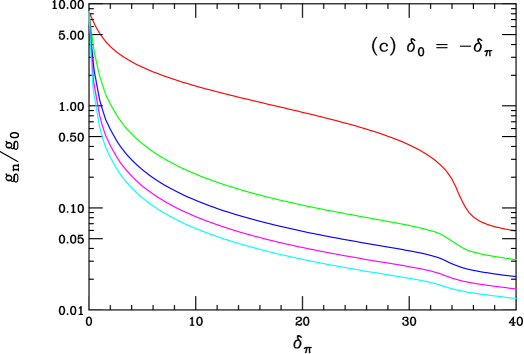
Figure 4: The ratios of the first five KK couplings to that of the zero-mode as a function of $\delta_{\pi}$ for the cases (a) $\delta_{0}=0$, (b) $\delta_{0}=\delta_{\pi}$, and (c) $\delta_{0}=-\delta_{\pi}$. The lightest (heaviest) KK mode corresponds to the top (bottom) curve in each case.

We can now compute the size of the effect of the brane localized kinetic terms on the ratio of couplings $g_{n}/g_{0}$. Using Eq.(18), we obtain

$$Z_{0}=1+\frac{\delta_{0}+\delta_{\pi}}{\pi kr_{c}}\,,$$ (27)

and, neglecting terms of order $\epsilon_{n}$,

$$Z_{n}\simeq 1+W^{-1}\left[2\delta_{\pi}+{8\delta_{0}\delta_{\pi}^{2}\alpha_{n}^{2}\over\pi^{2}\zeta_{0}^{2}(x_{n})}\right]\,.$$ (28)

Note that similar to the case of TeV^-1-sized extra dimensions, $Z_{n}$ is found to be $n$-dependent. From the requirement that $Z_{0}>0$, we obtain the constraint $\delta_{0}+\delta_{\pi}>-\pi kr_{c}\simeq-35.4$. If this condition isn’t satisfied, the state then has negative norm and is unphysical.

We first consider the case $\delta_{\pi}\geq 0$, in order to avoid the ghost states. Figures 4a-c display the existence of a significant fall-off of the ratio of couplings $g_{n}/g_{0}$ as a function of $\delta_{\pi}$. The values of the coupling ratio in the negative $\delta_{\pi}$ region, away from the regions where the ghost states appear, are shown in Fig. 5a-c. In both cases we see the mode dependence of the coupling strength away from the value $\delta_{\pi}=0$. Note that the coupling strength of the first KK excitation is substantially smaller when $\delta_{\pi}<0$ compared to the case with positive values of $\delta_{\pi}$. It is clear that compared to the original RS framework, the ratio $g_{n}/g_{0}$ is now naturally much reduced.

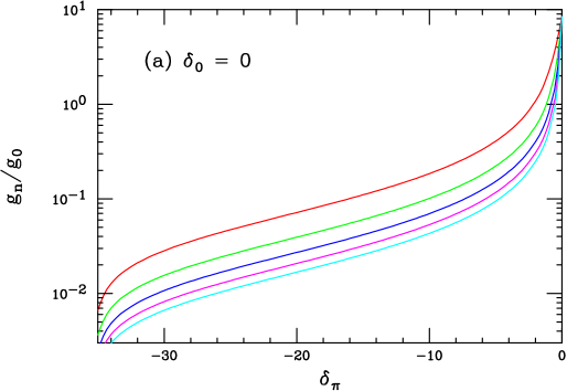
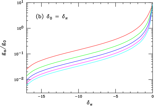
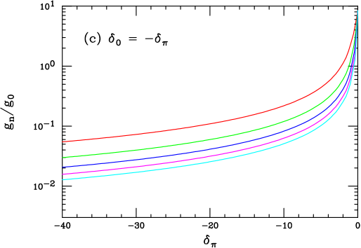
Figure 5: The ratios of the first five KK couplings to that of the zero-mode as a function of negative $\delta_{\pi}$ for the cases (a) $\delta_{0}=0$, (b) $\delta_{0}=\delta_{\pi}$, and (c) $\delta_{0}=-\delta_{\pi}$. The lightest (heaviest) KK mode corresponds to the top (bottom) curve in each case.

Due to the shifts in the mass spectrum and the reduced values of the ratio $g_{n}/g_{0}$, we now expect that the inclusion of the localized kinetic terms can result in a significant loosening of the precision electroweak bounds [4] on the RS model. To obtain the constraints on the KK gauge boson mass spectrum, we need to consider the quantity

$$\tilde{V}(\delta_{\pi},\delta_{0})\equiv\sum_{n}\Big{(}{g_{n}\over g_{0}}\Big{)}^{2}\Big{(}{x_{1}\over x_{n}}\Big{)}^{2}\,,$$ (29)

where the $x_{n}$ are the roots given above, and examine its detailed dependence on $\delta_{0,\pi}$. This quantity describes the relative strength of the set of contact interactions induced by dimension-6 operators arising from KK gauge exchanges in precision electroweak observables [4]; a full description of the analysis procedure and the dependence of the precision electroweak variables on $V$ can be found in Ref. [13]. Here, we perform a global fit to the most recent precision electroweak data sample [14] with the use of ZFITTER. Since for the case $\delta_{0,\pi}=0$ we know from our previous analysis that precision measurements imply the bound $m_{1}|_{RS}\mathrel{\mathchoice{\lower 3.01385pt\vbox{\halign{$\matth\displaystyle\hfil#\hfil$\cr>\crcr\sim\crcr}}}{\lower 3.01385pt\vbox{\halign{$\matth\textstyle\hfil#\hfil$\cr>\crcr\sim\crcr}}}{\lower 3.01385pt\vbox{\halign{$\matth\scriptstyle\hfil#\hfil$\cr>\crcr\sim\crcr}}}{\lower 3.01385pt\vbox{\halign{$\matth\scriptscriptstyle\hfil#\hfil$\cr>\crcr\sim\crcr}}}}25$ TeV for the lightest gauge KK excitation [4], we can easily obtain the corresponding constraint for non-zero values of $\delta_{0,\pi}$. We obtain the bound $m_{1}|_{BLKT}\geq m_{1}|_{RS}[\tilde{V}(\delta_{\pi},\delta_{0})/\tilde{V}(0,0)]^{1/2}$; the numerical results of this analysis is presented in Fig. 6a-b. Here, we see that the bound on $m_{1}$ falls rapidly as the magnitude of $\delta_{\pi}$ increases. For example, with $\delta_{\pi}\sim 10-20$, we see that $m_{1}$ can be as low as $2-3$ TeV which will lead to an observable signal in Drell-Yan production for the first gauge KK excitation at the LHC. This is demonstrated in Fig 7 for the case of $m_{1}=5$ TeV. For larger values of $\delta_{\pi}$, such states may be observable at the Tevatron. For $\delta_{\pi}<0$ away from the ghost root region, the constraints from electroweak data are even weaker; here, direct searches at the Tevatron can place bounds on the parameter space.

So far, we have shown that the inclusion of boundary kinetic terms allow for a substantially lighter mass spectrum for the gauge KK states than in the conventional RS scenario. However, the question remains as to whether this ameilorates the stringent bound of $\Lambda_{\pi}\mathrel{\mathchoice{\lower 3.01385pt\vbox{\halign{$\matth\displaystyle\hfil#\hfil$\cr>\crcr\sim\crcr}}}{\lower 3.01385pt\vbox{\halign{$\matth\textstyle\hfil#\hfil$\cr>\crcr\sim\crcr}}}{\lower 3.01385pt\vbox{\halign{$\matth\scriptstyle\hfil#\hfil$\cr>\crcr\sim\crcr}}}{\lower 3.01385pt\vbox{\halign{$\matth\scriptscriptstyle\hfil#\hfil$\cr>\crcr\sim\crcr}}}}100$ GeV. To address this issue, we convert the constraint on $m_{1}$ into one on $\Lambda_{\pi}$ by noting that $m_{1}=x_{1}\Lambda_{\pi}k/\overline{M}_{Pl}$, recalling that $k/\overline{M}_{Pl}\leq 0.1$, and using the values of $x_{1}$ that we computed above. Solving for $\Lambda_{\pi}$, we find the results displayed in Fig. 8. Note that for most values of the parameters, the resulting bound on $\Lambda_{\pi}$ remains quite large for positive values of $\delta_{\pi}$. This is due to the interplay of the modified roots and the constraints on the gauge KK mass spectrum. However, for $\delta_{\pi}<0$, we see that the lower bound on $\Lambda_{\pi}$ is easily reduced by almost an order of magnitude or more. This would seem to be the preferred region of parameter space for this model in its relation to the hierarchy problem.

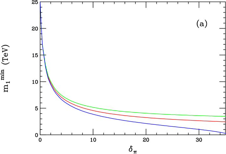
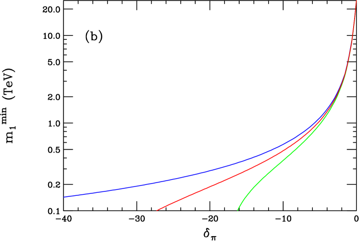
Figure 6: (a) Lower bound on the mass of the lightest gauge boson KK excitation as a function of $\delta_{\pi}\geq 0$ from a fit to the precision electroweak data for the cases $\delta_{0}=\delta_{\pi}$ (top/green), $\delta_{0}=0$ (middle/red), and $\delta_{0}=-\delta_{\pi}$ (bottom/blue). (b) Same as above but now for the region $\delta_{\pi}\leq 0$ with $\delta_{0}=\delta_{\pi}$ (bottom/green), $\delta_{0}=0$ (middle/red), and $\delta_{0}=-\delta_{\pi}$ (top/blue).

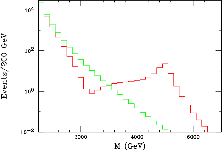
Figure 7: Drell-Yan event rate at the LHC for the first gauge KK state in the RS scenario with boundary terms. We have assumed a luminosity of 300  ${\mathrm{fb}}^{-1}$ and have set $m_{1}=5$ TeV. The steeply falling histogram represents the SM Drell-Yan continuum.

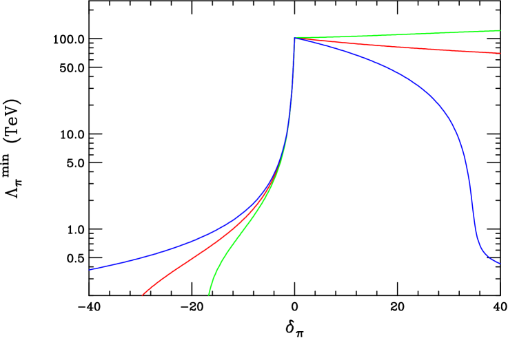
Figure 8: Bounds on $\Lambda_{\pi}$ as a function of $\delta_{\pi}$ for the cases $\delta_{0}=\delta_{\pi}$ (green), $\delta_{0}=0$ (red), and $\delta_{0}=-\delta_{\pi}$ (blue), as derived from the constraints on the mass of the first gauge KK state. The color coding of the curves corresponds to $\delta_{0}=\delta_{\pi}\,,0\,,-\delta_{\pi}$ being represented by the top(bottom), middle(middle), bottom(top) curves on the right(left) handside of the figure.

4 Conclusions

A minimal, yet interesting, extension of the RS model is obtained by assuming that only gauge fields propagate in the bulk. However, this setup has been shown to be constrained by precision electroweak data to have a scale $\Lambda_{\pi}\,\,\hbox to0.0pt{\raise 3.0pt\hbox{$>$}\hss}{\lower 3.0pt\hbox{$\sim$}}\,\,100$ TeV for physics on the TeV brane [4]. This makes such a scenario less attractive as a means for resolving the gauge hierarchy. The stringent bound on the electroweak scale $\Lambda_{\pi}$ is a result of the strong coupling of the gauge KK modes to the boundary fermions. It is thus interesting to examine if a modification of the boundary physics can lead to a relaxation of this constraint. One such possibility which is a simple extension of the theory, motivated by field theoretic considerations [8], is the addition of brane localized kinetic terms for the bulk gauge fields.

In this paper, we assumed the presence of localized gauge field kinetic terms on both the Planck and TeV branes in the RS model. We then derived the wavefunctions and the mass spectrum of the gauge KK modes. The couplings of the KK states to the SM brane localized fermions were then calculated. It was shown that for natural choices of parameters, a substantial suppression of these KK couplings, compared to the original model, can be achieved. We then reexamined the precision electroweak bounds on the lightest gauge KK mass or, equivalently, $\Lambda_{\pi}$. We found that for a reasonably wide range of parameters, the mass of the lightest gauge KK field can be as low as a few hundred GeV and hence will be visible at the LHC and possibly the Tevatron. The weakening of the constraints from precision data results in a significantly less severe bound on $\Lambda_{\pi}$; one can now naturally obtain $\Lambda_{\pi}\,\,\hbox to0.0pt{\raise 3.0pt\hbox{$<$}\hss}{\lower 3.0pt\hbox{$\sim$}}\,\,10$ TeV. This makes the RS framework with gauge fields in the bulk more favorable, in the context of a solution to the hierarchy problem, and facilitates the construction of more realistic models based on the RS proposal. In addition, for much of the $\delta_{0,\pi}$ parameter space, the gauge field and graviton KK excitations are nearly degenerate which may result in some interesting collider phenomenology.

Given the observations in this paper, we expect that the addition of brane localized kinetic terms for other bulk fields, such as gravitons, could significantly alter the phenomenology of the RS model, and could also lead to the appearance of new features in the low energy theory.

Acknowledgements

The work of H.D. was supported by the US Department of Energy under contract DE-FG02-90ER40542.

Note Added: A related article appeared at a similar time [15]; we thank these authors for pointing out a sign error in an earlier version of this manuscript.

Appendix

Here, we will show that near special values of the BLKT coefficients $\delta_{0}$ and $\delta_{\pi}$ a vanishing root develops in Eq.(15), signaling the appearance of an unphysical ghost state. We will also discuss the large $|\delta_{\pi}|$ limit of this equation. In the limit where $x_{n}\rightarrow 0$, Eqs.(15) and (16) yield

$$x_{n}^{2}=\frac{-4(\delta_{\pi}+\delta_{0}+kr_{c}\pi)}{-(kr_{c}\pi+\delta_{0})(2\delta_{\pi}+1)+(1+\delta_{\pi})}.$$ (30)

This equation is valid for $x_{n}\ll 1$, and for $\delta_{\pi}=-(\delta_{0}+kr_{c}\pi)$, it yields $x_{n}^{2}=0$. Thus, for $\delta_{\pi}\leq-(\delta_{0}+kr_{c}\pi)$, an unphysical ghost state, a state with negative norm, appears in the spectrum, as implied by Eq. (27). Note that in the original RS model, with $\delta_{0}=\delta_{\pi}=0$, this ghost state does not appear, since $kr_{c}\pi>0$.

We now study Eq.(30) in the limit $\delta_{\pi}\rightarrow\pm\infty$, for the three cases $\delta_{0}=0,\delta_{\pi},-\delta_{\pi}$ that were examined in the text. For $\delta_{0}=0$, we have $x_{n}^{2}\rightarrow 4/(2kr_{c}\pi-1)$ as $\delta_{\pi}\rightarrow\pm\infty$. Since $kr_{c}\pi\approx 35$, the small $x_{n}$ approximation is valid and for $\delta_{\pi}\rightarrow+\infty$, the root is physical, as shown in Fig. 1a. Here, we see that the root for the lowest KK state asymptotes to a constant value of $\simeq 0.24$ as $\delta_{\pi}$ becomes large and positive; when $\delta_{\pi}$ is large and negative, the ghost root asymptotes to this same value. For $\delta_{0}=\delta_{\pi}$, $x_{n}^{2}\rightarrow 4/\delta_{\pi}$ as $\delta_{\pi}\rightarrow\pm\infty$. This root is only physical for $\delta_{\pi}\rightarrow+\infty$, and approaches zero, as presented in Fig. 2a. In the case where $\delta_{0}=-\delta_{\pi}$, we have $x_{n}^{2}\rightarrow-(4kr_{c}\pi)/(2\delta_{\pi}^{2})$ as $\delta_{\pi}\rightarrow\pm\infty$, and there are no light physical modes in this limit, as seen in Fig. 2b.

We would like to note that in the limit $\delta_{\pi}\rightarrow\pm\infty$, with choices of $\delta_{0}$ that yield $|\alpha_{n}|\ll 1$, Eq.(15) is well-approximated by $J_{1}(x_{n})=0$, for $x_{n}\neq 0$. In this case, apart from the special light modes discussed above, the rest of the gauge field KK modes have masses that are approximately degenerate with those of the KK gravitons from the original RS model [3]. More generally, as can be seen from Figures 1a and 2, a large range of parameters exist where this near degeneracy occurs. This will have important phenomenological implications at future colliders.

References

- [1] L. Randall and R. Sundrum, Phys. Rev. Lett. 83, 3370 (1999) [arXiv:hep-ph/9905221].
- [2] W. D. Goldberger and M. B. Wise, Phys. Rev. Lett. 83, 4922 (1999) [arXiv:hep-ph/9907447].
- [3] H. Davoudiasl, J. L. Hewett and T. G. Rizzo, Phys. Rev. Lett. 84, 2080 (2000) [arXiv:hep-ph/9909255].
- [4] H. Davoudiasl, J. L. Hewett and T. G. Rizzo, Phys. Rev. D 63, 075004 (2001) [arXiv:hep-ph/0006041] and Phys. Lett. B 473, 43 (2000) [arXiv:hep-ph/9911262].
- [5] A. Pomarol, Phys. Lett. B 486, 153 (2000)[arXiv:hep-ph/9911294]; Y. Grossman and M. Neubert, Phys. Lett. B 474, 361 (2000) [arXiv:hep-ph/9912408]; T. Gherghetta and A. Pomarol, Nucl. Phys. B 586, 141 (2000); S. Chang, J. Hisano, H. Nakano, N. Okada and M. Yamaguchi, Phys. Rev. D 62, 084025 (2000)[arXiv:hep-ph/9912498]; R. Kitano, Phys. Lett. B 481, 39 (2000)[arXiv:hep-ph/0002279]; S. J. Huber and Q. Shafi, Phys. Lett. B 498, 256 (2001) [arXiv:hep-ph/0010195] and Phys. Rev. D 63, 045010 (2001) [arXiv:hep-ph/0005286]; S. J. Huber, C. A. Lee and Q. Shafi, arXiv:hep-ph/0111465; J. L. Hewett, F. J. Petriello and T. G. Rizzo, JHEP 0209, 030 (2002) [arXiv:hep-ph/0203091]; F. Del Aguila and J. Santiago, arXiv:hep-ph/0111047, arXiv:hep-ph/0011143, Nucl. Phys. Proc. Suppl. 89, 43 (2000)[arXiv:hep-ph/0011142] and Phys. Lett. B 493, 175 (2000)[arXiv:hep-ph/0008143]; C. S. Kim, J. D. Kim and J. Song, arXiv:hep-ph/0204002; C. Csaki et al., Phys. Rev. D66, 064021 (2002), hep-ph/0203034; G. Burdman, Phys. Rev. D 66, 076003 (2002) [arXiv:hep-ph/0205329]; F. del Aguila and J. Santiago, arXiv:hep-ph/0212205.
- [6] W. D. Goldberger and M. B. Wise, Phys. Rev. D 60, 107505 (1999) [arXiv:hep-ph/9907218].
- [7] M. Carena, T. Tait and C. Wagner, hep-ph/0207056.
- [8] H. Georgi, A.K. Grant and G. Hailu, Phys. Lett. B506, 207 (2001).
- [9] H.C. Cheng, K.T. Matchev and M. Schmaltz, hep-ph/0204342 and hep-ph/0205314.
- [10] L. Hall and Y. Nomura Phys. Rev. D64, 055003 (2001)and Phys. Rev. D65, 125012 (2002); Y. Nomura, Phys. Rev. D65, 085036 (2002); R. Contino, L. Pilo, R. Rattazzi and E. Trincherini, Nucl. Phys. B622, 227 (2002); M. Chaichian and A. Kobakhidze, hep-ph/0208129.
- [11] K. Agashe and A. Delgado, [arXiv:hep-th/0209212]; K. Agashe, A. Delgado and R. Sundrum, Nucl. Phys. B 643, 172 (2002) [arXiv:hep-ph/0206099].
- [12] G.R. Davali, G. Gabadadze and M. Porrati, Phys. Lett. B485, 208 (2000); G.R. Davali and G. Gabadadze, Phys. Rev. D63, 065007 (2001); G.R. Davali, G. Gabadadze and M.A. Shifman, Phys. Lett. B497, 271 (2001); G.R. Davali, G. Gabadadze and M. Kolanovic, Phys. Rev. D64, 084004 (2001); S.L. Dubovsky and V.A. Rubakov, Int. J. Mod. Phys. A16, 4331 (2001); M. Chaichian and A.B. Kobakhidze, Phys. Rev. Lett. 87, 171601 (2001); M.Carena et al., Nucl. Phys. 609, 499 (2001).
- [13] T. G. Rizzo and J. D. Wells, Phys. Rev. D 61, 016007 (2000) [arXiv:hep-ph/9906234].
- [14] M. Grünewald, talk presented at the 31st International Conference on High Energy Physics, Amsterdam, Netherlands, July 2002; LEP/SLD Electroweak Working Group, LEPEWWG/2002-01.
- [15] M. Carena, E. Ponton, T. Tait and C. E. Wagner, arXiv:hep-ph/0212307.