Full one-loop electroweak radiative corrections to single Higgs production in $e^{+}e^{-}\;$.

G. Bélanger¹⁾, F. Boudjema¹⁾, J. Fujimoto²⁾, T. Ishikawa²⁾,

T. Kaneko²⁾, K. Kato³⁾, Y. Shimizu²⁾

1) LAPTH${\;}^{\dagger}$, B.P.110, Annecy-le-Vieux F-74941, France.

2) KEK, Oho 1-1, Tsukuba, Ibaraki 305–0801, Japan.

3) Kogakuin University, Nishi-Shinjuku 1-24, Shinjuku, Tokyo 163–8677, Japan.

Abstract

We present the full ${{\cal O}}(\alpha)$ electroweak radiative corrections to single Higgs production in $e^{+}e^{-}\;$. This takes into account the full one-loop corrections as well as the effects of hard photon radiation. We include both the fusion and Higgs-strahlung processes. The computation is performed with the help of GRACE-loop where we have implemented a generalised non-linear gauge fixing condition. The latter includes $5$ gauge parameters that can be used for checks on our results. Besides the UV, IR finiteness and gauge parameter independence checks it proves also powerful to test our implementation of the 5-point function. We find that for a 500GeV machine and a light Higgs of mass $150$GeV, the total ${{\cal O}}(\alpha)$ correction is small when the results are expressed in terms of $\alpha_{{\rm QED}}$. The total correction decreases slightly for higher energies. For moderate centre of mass energies the total ${{\cal O}}(\alpha)$ decreases as the Higgs mass increases, reaching $-10\%$ for $M_{H}=350$GeV and $\sqrt{s}=500$GeV. In order to quantify the genuine weak corrections we have subtracted the universal virtual and bremsstrahlung correction from the full ${{\cal O}}(\alpha)$. We find, for $M_{H}=150$GeV, a weak correction slowly decreasing from $-2\%$ to $-4\%$ as the energy increases from $\sqrt{s}=300$GeV to $\sqrt{s}=1$TeV after expressing the tree-level results in terms of $G_{\mu}$.

LAPTH-959/2002

KEK-CP-135

^†UMR 5108 du CNRS, associée à l’Université de Savoie.

1 Introduction

Uncovering the mechanism of symmetry breaking is one of the major tasks of the high energy colliders. Most prominent is the search for the Higgs particle. Although the LHC should not miss this particle even if it weighed up to 1TeV, precision measurements on the Higgs properties will only be conducted in an $e^{+}e^{-}\;$collider. There are two important mechanisms for Higgs production in $e^{+}e^{-}\;$. The Higgs-strahlung process, $e^{+}e^{-}\;\rightarrow ZH\;$and the $W$-fusion process, $e^{+}e^{-}\;\rightarrow\nu_{e}\bar{\nu}_{e}H\;$. The former is the dominant one at small (in the LEP2 range say) to moderate energies but decreases rather fast with energy. At TeV energies the $W$-fusion process dominates by far for Higgs masses up to $1$TeV. Even at $500$GeV this $t$-channel process is dominant for Higgs masses in the range preferred by the indirect electroweak precision data[1] and remains an important component for all Higgs masses at energies of the linear collider. Tree-level computations of Higgs production are rather well under control[2, 3], including interference of the $W$ fusion process with the Higgs-strahlung process. Note however that the complexity of the process $e^{+}e^{-}\;\rightarrow\nu\bar{\nu}H\;$precludes a full analytic result for the total cross section even at tree-level, although the differential cross section can be cast in a very compact form[2, 3]. Full radiative corrections for Higgs-strahlung have been considered by a number of groups[4], while a proper one-loop treatment of the fusion process is still lacking despite the importance of the process for the linear collider physics program. Some recipes have been suggested[5, 6] to include parts of the radiative corrections to the fusion process but considering the domain of validity of these approximations $\sqrt{s},M_{H}\ll 2m_{t}$, they are expected not to be precise for the interesting range of Higgs masses(preferred by the latest precision measurements[1]) and next collider energies. One-loop contribution to the $HWW$ vertex has been considered on the basis that it might constitute a good approximation for the fusion process[7], but it rests to see how well this approximation fares in comparison of the full calculation. Very recently one-loop radiative corrections to this process have been investigated within the minimal supersymmetric model but again by only taking into account the contribution of the fermions and sfermions to the $H/hWW$ vertex[7, 8]. It is the aim of this letter to summarise the results of the full radiative corrections to single Higgs production in $e^{+}e^{-}\;$, including both the fusion and Higgs-strahlung processes in the ${\cal{S}}{\cal{M}}\;$(Standard Model). We include both the virtual and soft corrections as well as the hard photon radiation. A longer paper will detail our computation and results and will look into the issue of finding approximations to the full result.

A standard hand calculation using the usual techniques could hardly be attempted for such $2\rightarrow 3$ processes at one-loop. Considering the ever increasing power of computers, the possibility of parallelisation and the fact that the whole procedure of perturbation theory consists of algorithms that can be directly translated on a computer it seems that most, if not all, complex calculations in high-energy physics can be automated. This is especially true for electroweak processes where various scales and masses enter the calculations. GRACE-loop [11] from which our results are derived is such a program. GRACE [12], the tree-level component of the system, has been tested and heavily used for tree-level cross sections up to 6-fermions in the final state[13]. GRACE-loop has been exploited and checked thoroughly for a variety of $2\rightarrow 2$ processes in the electroweak theory [14]. The system which requires as input, a model file that describes all the interaction vertices derived from a particular Lagrangian can generate all the necessary Feynman graphs together with their codes so that matrix elements can be generated before being processed for the calculation of the cross section and event generation. For loop processes, there is a symbolic manipulation stage (either FORM[15] or REDUCE[16] ) that handles all the Dirac and tensor algebra in $n$-dimension for all the interference terms between tree-level and 1-loop diagrams and automatically applies the Feynman trick for the propagator. This is then passed to a module that contains two libraries for the loop integration containing the FF package[17] as well as an in-house numerical code. The system together with the one-loop renormalisation program is described in detail in [14]. As far as the calculation of one-loop processes is concerned, a series of powerful tests are implemented in the code as described in [14] and as will be presented below for $e^{+}e^{-}\;\rightarrow\nu\bar{\nu}H\;$.

2 Tree-level results, setting-up the loop calculation

Our input parameters for the calculation of $e^{+}e^{-}\;\rightarrow\nu\bar{\nu}H\;$are the following. Throughout we expressed our results in terms of the fine structure constant in the Thomson limit $\alpha^{-1}=137.0359895$ and the $Z$ mass $M_{Z}=91.1876$GeV. Our on-shell renormalisation program uses $M_{W}$ as input parameter, nonetheless our numerical value of $M_{W}$ is derived through $\Delta r$[18]. $M_{W}$ thus changes as a function of $M_{H}$. For the the lepton masses we take $m_{e}=0.510999$MeV, $m_{\mu}=105.6584$MeV and $m_{\tau}=1.777$GeV. For the quark masses beside the top mass $M_{t}=174$GeV, we take the set $M_{u}=M_{d}=58$MeV, $M_{s}=92$MeV, $M_{c}=1.5$GeV and $M_{b}=4.7$GeV. With these values we calculate $\Delta\alpha(M_{Z})=0.059258$. With this we find for example that $M_{W}=80.3767$GeV for $M_{H}=150$GeV and $M_{W}=80.3158$GeV for $M_{H}=350$GeV. Especially for the Higgs-strahlung subprocess we require a $Z$-width. We have taken a constant fixed $Z$-width, $\Gamma_{Z}=2.4952$GeV. Unless when otherwise stated our results refer to the full $e^{+}e^{-}\;\rightarrow\nu\bar{\nu}H\;$, summing over all three types of neutrinos with, for electron neutrinos, the effect of interference between fusion and Higgs-strahlung.

We have checked that our tree-level results are in very good agreement with those in [2] after expressing them in terms of $G_{\mu}$. However since we are considering the effect of radiative corrections, within our scheme we prefer showing all our results using $\alpha$. We will only comment on the $G_{\mu}$ scheme at the end of this letter. We find for example for $\sqrt{s}=500$GeV and $M_{H}=350$GeV that $\sigma_{{\rm tree,total}}=4.606$fb at tree-level for the contribution of all three neutrinos. In an attempt to separate the different contributions to single Higgs production, we will refer to the $s$-channel as given by $\sigma_{s}=3\times\sigma(e^{+}e^{-}\;\rightarrow\nu_{\mu}\bar{\nu}_{\mu}H)$. The bulk of this contribution is given by $\sigma(e^{+}e^{-}\;\rightarrow ZH)\times B_{Z\rightarrow{\rm inv.}}\;,\;B_{Z\rightarrow{\rm inv.}}\simeq 20\%$. We will define the $t$-channel as $\sigma_{t}=\sigma_{{\rm total}}-\sigma_{s}$, this implicitly means that the interference term is included in this contribution. These definitions will be carried over to the one-loop case as well.

In Fig. 2 we have also included the tree-level cross section. They are shown as a function of the centre-of-mass energy for a light Higgs of mass $M_{H}=150$GeV as well as a function of the Higgs mass at a centre-of-mass of $500$GeV. All integration over phase space are done with the help of BASES, see[12]. These figures clearly show the importance of the $t$-channel contribution pointed out in the introduction. For a low Higgs mass of $150$GeV, although the $s$-channel still dominates at $\sqrt{s}=300$GeV, very quickly at $\sqrt{s}=500$GeV it is the $t$-channel that dominates. For the latter energy as the Higgs mass increases, the $t$-channel contribution drops much quickly than the $s$-channel, where both merge around $M_{H}=380$GeV to $M_{H}=390$GeV, but very quickly around the $ZH$ threshold for $M_{H}\sim 408$GeV, the $s$-channel drops precipitously leaving the $t$-channel as the sole contribution for the whole process.

Figure 1: A small selection of different classes of loop diagrams contributing to $e^{+}e^{-}\;\rightarrow\nu\bar{\nu}H\;$. We keep the same graph numbering as that produced by the system. Graph 1312 belongs to the corrections from self-energies, here both the virtual and counterterm contributions are generated and counted as one diagram. Graph 87 shows a vertex correction. Both graphs can be considered as resonant Higgs-strahlung contributions. Graph 249 represents a box correction, it is a non resonant contribution but applies also to the $\nu_{\mu},\nu_{\tau}$ channels. Graph 486 is also a box correction which is non resonant and applies only to $\nu_{e}$. Graph 541 and Graph 565 are typical bosonic and fermionic corrections to the $WWH$ vertex for the fusion process. Graph 846 shows a pentagon correction that also applies to $\mu$ and $\tau$ neutrinos, this again can be considered as a non-resonant contribution. Graphs 827 and 828 are pentagons that only contribute to $e^{+}e^{-}\;\rightarrow\nu_{e}\bar{\nu}_{e}H\;$.

Neglecting all Goldstone-electron coupling (proportional to the electron mass), one has at one-loop $249$ diagrams (for $\nu_{e}\bar{\nu}_{e}H$, and $146$ for $\nu_{\mu}\bar{\nu}_{\mu}H$) including $15$ pentagons (5-point functions) compared to only 2 diagrams at tree-level, one for the fusion process and one for the Higgs-strahlung. Keeping the electron Yukawa coupling one has a total of $1350$ diagrams (98 pentagons corresponding to 5-point functions) at one-loop. Although in running our program to derive cross sections we only use the set of 249 diagrams, to perform our extensive checks especially those of gauge-parameter independence, at the level of the differential cross section, we keep the full set of 1350 diagrams. It is impossible to show all the contributing diagrams here. They may be downloaded or visualised at this location[19]. All these diagrams are generated and drawn by gracefig the Feynman diagrams generator of GRACE . A representative selection of diagrams is shown in Fig. 1.

The results of the calculation are checked by performing three kinds of tests at some random points in phase space. For these tests to be passed one works in quadruple precision. We first check the ultraviolet finiteness of the results. This test applies to the whole set of the virtual one-loop diagrams. In order to conduct this test we regularise any infrared divergence by giving the photon a fictitious mass (we set this at $\lambda=10^{-15}$GeV). In the intermediate step of the symbolic calculation dealing with loop integrals (in $n$-dimension), we extract the regulator constant $C_{UV}=1/\varepsilon-\gamma_{E}+\log 4\pi$, $n=4-2\varepsilon$ and treat this as a parameter. The ultraviolet finiteness test gives a result that is stable over $30$ digits when one varies the dimensional regularisation parameter $C_{UV}$. This parameter could then be set to $0$ in further computation. The test on the infrared finiteness is performed by including both loop and bremsstrahlung contributions and checking that there is no dependence on the fictitious photon mass $\lambda$. We find results that are stable over $23$ digits when varying $\lambda$. An additional test concerns the bremsstrahlung part. It relates to the independence in the parameter $k_{c}$ which is a soft photon cut parameter that separates soft photon radiation and the hard photon performed by the Monte-Carlo integration.

Gauge parameter independence of the result is performed through a set of five gauge fixing parameters. For the latter a generalised non-linear gauge fixing condition[20] has been chosen.

$${{\cal L}}_{GF} = -\frac{1}{\xi_{W}}|(\partial_{\mu}\;-\;ie\tilde{\alpha}A_{\mu}\;-\;igc_{W}\tilde{\beta}Z_{\mu})W^{\mu+}+\xi_{W}\frac{g}{2}(v+\tilde{\delta}H+i\tilde{\kappa}\chi_{3})\chi^{+}|^{2}$$ (2.1)

$$\;-\frac{1}{2\xi_{Z}}(\partial.Z+\xi_{Z}\frac{g}{2c_{W}}(v+\tilde{\varepsilon}H)\chi_{3})^{2}\;-\frac{1}{2\xi_{A}}(\partial.A)^{2}\;.$$

The $\chi$ represent the Goldstone. We take the ’t Hooft-Feynman gauge with $\xi_{W}=\xi_{Z}=\xi_{A}=1$ so that no “longitudinal” term in the gauge propagators contributes. Not only this makes the expressions much simpler and avoids unnecessary large cancelations, but it also avoids the need for high tensor structures in the loop integrals. The use of five parameters is not redundant as often these parameters check complementary sets of diagrams. For example the parameter $\tilde{\beta}$ is involved in all diagrams containing the gauge $WWZ$ and their Goldstone counterpart, whereas $\tilde{\alpha}$ checks $WW\gamma$ and $\tilde{\delta}$ is implicitly present in $WWH$. For each parameter of the set $\zeta=(\tilde{\alpha},\tilde{\beta},\tilde{\delta},\tilde{\kappa},\tilde{\epsilon})$ the first check is made while freezing all other four parameters to $0$. We have also made checks with two parameters non-zero. In principle checking for $2$ or $3$ values of the gauge parameter should be convincing enough. We in fact go one step further and perform a complete gauge parameter independence. To achieve this we generate for each non-linear gauge parameter $\zeta$, the values of the loop correction to the total differential cross section as well as the contribution of each one-loop diagram contribution for the five values $\zeta=0,\pm 1,\pm 2$. The one-loop diagram contribution from each loop graph $g$, is defined as

$${\rm d}\sigma_{g}={\rm d}\sigma_{g}(\zeta)=\Re\left({{\cal T}}^{loop}_{g}\cdot{{\cal T}}^{tree\ \dagger}\right)\;.$$ (2.2)

${{\cal T}}^{tree}$ is the tree-level amplitude summed over all tree-diagrams. ${{\cal T}}^{loop}_{g}$ is the one-loop amplitude contribution of the one-loop diagram $g$. A rapid look at the structure of the Feynman rules of the non-linear gauge leads one to conclude that for $e^{+}e^{-}\;\rightarrow\nu\bar{\nu}H\;$each contribution is a polynomial of (at most) third degree in the gauge parameter and thus, that each contribution, ${\rm d}\sigma_{g}$ may be written as

$${\rm d}\sigma_{g}={\rm d}\sigma_{g}^{(0)}+\zeta{\rm d}\sigma_{g}^{(1)}+\zeta^{2}{\rm d}\sigma_{g}^{(2)}+\zeta^{3}{\rm d}\sigma_{g}^{(3)}\;,$$ (2.3)

For each contribution ${\rm d}\sigma_{g}$, it is a straightforward matter, given the values of ${\rm d}\sigma_{g}$ for the five input $\zeta=0,\pm 1,\pm 2$, to reconstruct ${\rm d}\sigma_{g}^{(0,1,2,3)}$. This is what we do. In fact for each set of parameters we automatically pick up all those diagrams that involve a dependence on the gauge parameter. The number of diagrams in this set depends on the parameter chosen. In some cases a very large number of diagrams is involved. For the process at hand this occurs with the parameter $\tilde{\delta}$ where about $500$ diagrams are involved in the check.

We then verify that the differential cross section is independent of $\zeta$

$${\rm d}\sigma=\sum_{g}{\rm d}\sigma_{g}=\sum_{g}{\rm d}\sigma_{g}^{(0)}\;,$$ (2.4)

and therefore that

$${\rm sum}_{i}=\frac{\sum_{g}{\rm d}\sigma_{g}^{(i)}}{{\rm Max}_{g}\bigl{(}|{\rm d}\sigma_{g}^{(i)}|\bigr{)}}\;\;,\;\;i=1,2,3\;,$$ (2.5)

vanishes.

	$\#$ graphs	${\rm sum}_{3}$	${\rm sum}_{2}$	${\rm sum}_{1}$
$\tilde{\alpha}$	149	$-$	$10^{-28}$	$10^{-30}$
$\tilde{\beta}$	314	$-$	$10^{-31}$	$10^{-23}$
$\tilde{\delta}$	477 (1059)	$10^{-20}$	$10^{-20}$	$10^{-26}$
$\tilde{\kappa}$	122	$-$	$10^{-23}$	$10^{-23}$
$\tilde{\epsilon}$	128 (132)	$-$	$10^{-21}$	$10^{-30}$

Table 1: Numerical size of sum_i for each non-linear gauge parameter. ’# of graphs’ means the number of graphs that contributes to each sum depending on the gauge parameter, the number between bracket include the residual dependence from ${{\cal T}}^{tree\ \dagger}$. $-$ means that no diagram is involved.

As seen from Table 1 agreement within $20$ to $30$ digits is observed. This agreement gets better if one gives the electron mass a higher value, say $1$GeV. The gauge parameter dependence check not only tests the various components of the input file (correct Feynman diagrams for example) but also the symbolic manipulation part and most important of all the correctness of all the reduction formulae and the proper implementation of all the $N$-point functions. This is quite useful when one deals with 5-point functions as is the case at hand. Talking of parametric integrals all tensor reductions are done following the standard procedure and then passing the scalar integrals to the FF package[17] or to our own specially optimised routines when photon exchange is involved. The pentagon integrals are expressed in terms of boxes as is now standard[21], our procedure is outlined in the Appendix. We work in the on-shell renormalisation scheme closely following [22]. Apart from masses and couplings, renormalisation is also carried for the fields. In particular we also require the residues of the renormalised propagators of all physical particles to be unity. As known[4], this procedure leads to a (very sharp) threshold singularity in the wave function of the Higgs at the thresholds corresponding to $M_{H}=2M_{W},2M_{Z}$. Solutions to smooth this behaviour[23], like the inclusion of the finite width of the $W$ and $Z$, do exist but we have not implemented them yet in the present version of GRACE-loop . Therefore when scanning over $M_{H}$ it is sufficient to avoid these regions within $1$GeV around the thresholds.

As a separate check on our implementation we have also computed $H\rightarrow WW$ and $e^{+}e^{-}\;\rightarrow ZH$, after tuning our parameters we find excellent agreement with the literature[4, 5].

3 Results

3.1 Full ${{\cal O}}(\alpha)$ results

The results we show here include all 3 neutrino species. We first discuss the full ${{\cal O}}(\alpha)$ which includes the hard bremsstrahlung part. The separation between the $s$-channel and the $t$-channel is done in the same way as with the separation done at tree-level. It should be noted that in the one-loop diagrams that contribute to $e^{+}e^{-}\;\rightarrow\nu_{\mu}\bar{\nu}_{\mu}H$, and which we classify as $s$-channel, there are diagrams which can not be deduced from the one-loop corrections to the $s$-channel $2\rightarrow 2$ process $e^{+}e^{-}\;\rightarrow ZH$. Graph 249 in Fig.1 is one example. The relative correction for all three contributions is defined as $\delta_{{{\cal O}}(\alpha)}\equiv\frac{\sigma_{O(\alpha)}}{\sigma_{tree}}-1$ and will be referred to as the full one-loop ${{\cal O}}(\alpha)$ correction.

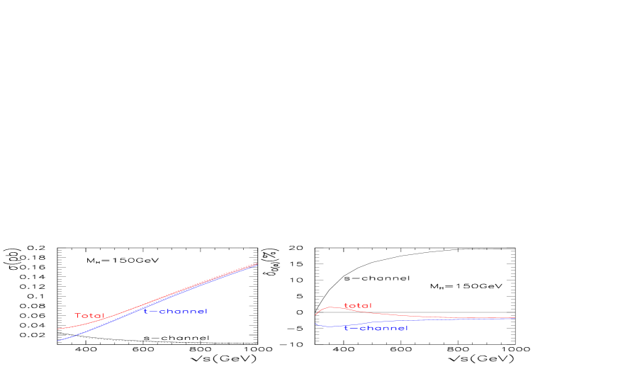
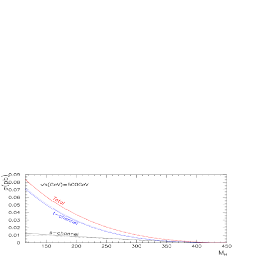
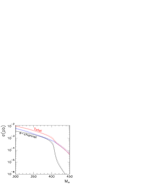
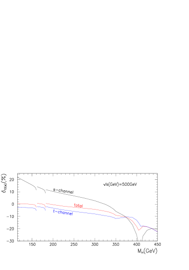
Figure 2: The two figures in the first row show the cross section as a function of centre-of-mass energy for a light Higgs of mass $M_{H}=150$GeV. We show the $s$-channel, $t$-channel and the sum of these (total) cross sections as defined in the text. Both the tree-level (dashed lines) and the full one-loop correction (full lines) are shown. In the second panel we show the relative correction in per-cent. In the second row, the dependence of the cross section as a function of the Higgs mass at a centre-of-mass of $500$GeV is shown.

One important remark is that the overall correction in the $s$-channel and $t$-channel are quite different. For a light Higgs of mass $150$GeV the correction to the $s$-channel Higgs-strahlung contribution is positive for practically all centre of mass energies of the next linear collider, see Fig. 2. It rises rather sharply to reach about $+20\%$ for a centre-of mass energy of 1TeV, however as will be argued below, the bulk of these large corrections are due to virtual and real QED corrections. Moreover in regions where these corrections are large, the Higgs-strahlung contribution is rather small. On the other hand the total correction in the $t$-channel for a small Higgs mass of 150GeV is negative throughout the range $\sqrt{s}=350$GeV to 1TeV, and is almost constant past $\sqrt{s}=500$GeV, reaching about $-2\%$. Combining these two contributions, we see that the full correction to the whole process also remains small for a small Higgs mass. In fact at $500$GeV it is almost at its lowest of about $0.2\%$. This is an accidental cancellation between the contributions of both the $t$-channel and the $s$-channel at this energy. We have also studied the Higgs mass dependence of the corrections. First of all note that all our results capture the sharp spikes for $M_{H}=2M_{W},2M_{Z}$, the top threshold is also visible when we plot the relative corrections. For $500$GeV the $s$-channel ${{\cal O}}(\alpha)$ correction decreases for higher Higgs masses, eventually turning negative with a value $-6\%$ for $M_{H}=350$GeV. It then drops rather sharply to reach as much as $-30\%$ at the $ZH$ threshold, past which this cross section is completely negligible. This behaviour is largely due to QED corrections and is driven by the kinematics of the two-body $e^{+}e^{-}\;\rightarrow ZH$. At $500$GeV the correction in the $t$-channel contribution remains negative for all Higgs masses that we considered, i.e. in the range $115-450$GeV. It drops steadily from about $-2\%$ for $M_{H}=115$GeV to about $-10\%$ at $350$GeV close to the top pair threshold. It then increases up to the $ZH$ threshold before dropping sharply around the $ZH$ threshold. Most of the large corrections are due to QED corrections.

3.2 Extraction the QED corrections

As is known large QED corrections require a higher order treatment. In order to quantify the effects of the genuine weak corrections, one could try subtract these QED corrections. This can be done rather easily for the $s$-channel contribution, where the correction can be readily extracted from the electromagnetic correction to the $eeZ$ vertex and the soft-photon bremsstrahlung part. Indeed our computation produces at an intermediate stage the result including the soft bremsstrahlung correction, that is before the inclusion of hard photons. The cut on the photon energy, $k_{c}$, has been taken sufficiently small, $k_{c}=0.1$GeV. These corrections without hard bremsstrahlung include thus the QED virtual and soft bremsstrahlung (which depend on $k_{c}$) as well as the genuine weak correction to the process. For this $s$-channel process the latter QED corrections are given by the universal soft photon factor that leads to a relative correction

$$\delta_{V+S}^{QED}=\frac{2\alpha}{\pi}\left((L_{e}-1)\ln\frac{k_{c}}{E_{b}}+\frac{3}{4}L_{e}+\frac{\pi^{2}}{6}-1\right)\;,\;L_{e}=\ln(s/m_{e}^{2})\;.$$ (3.6)

where $m_{e}$ is the electron mass and $E_{b}$ the beam energy $s=4E_{b}^{2}$. Subtracting this contribution from our $k_{c}$ dependent (numerical) result reproduces the genuine weak correction, $\delta_{W,s-channel}$.

To quantify in an unambiguous way the effect of the weak correction in the $t$-channel we have also subtracted this universal factor $\delta_{V+S}^{QED}$ from the full ${{\cal O}}(\alpha)$ correction. It can be shown that the leading (infrared and collinear) contributions are given by the universal factor, Eq. 3.6[14]. This procedure also paves the way to a resummation of these large QED factors for the full process which is conducive to a Monte-Carlo implementation as could be done for instance through a QED parton shower[24]. This will be treated elsewhere. Coming back to the weak corrections, we will denote by $\delta_{W,t-channel}$ and $\delta_{W,total}$ the weak correction for the $t$-channel and the full process based on the subtraction of the universal QED factor in Eq. 3.6.

For a light Higgs mass ($M_{H}=150$GeV), the weak correction for the $s$ and $t$-channels have a different behaviour as the energy increases, see Fig. 3. The former varies from about $6\%$ at $\sqrt{s}=300$GeV to $-2.5\%$ at $\sqrt{s}=1$TeV. Past $400$GeV where it dominates, the weak correction to the $t$-channel varies rather slowly from $7\%$ at $\sqrt{s}=400$GeV to about $5\%$ at $\sqrt{s}=1$TeV. The dependence of the weak corrections on the Higgs mass for a moderate centre-of-mass energy, $\sqrt{s}=500$GeV, reveals that up to the $ZH$ threshold these corrections increase with the Higgs mass (most probably due to $M_{H}^{2}$ terms from the Higgs self-coupling as in $e^{+}e^{-}\;\rightarrow ZH$), apart from the clearly visible spikes at the $W,Z$ and the top thresholds. Apart from the drop in the $t$-channel contribution around the $ZH$ threshold, the weak correction in the $t$-channel picks up again and as expected merges with the correction to the full process.

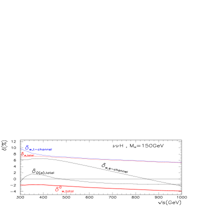
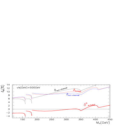
Figure 3: Relative weak corrections as defined in the text, for the $t$-channel ($\delta_{W,t-channel}$), $s$-channel ($\delta_{W,s-channel}$)and the whole process ($\delta_{W,total}$). We also show the full ${\cal O}(\alpha)$ correction for the whole process in the first panel. Also shown is the weak correction for the full process expressed in the $G_{\mu}$ scheme ($\delta^{G}_{w,total}$), see text.

3.3 Expressing the weak corrections in terms of $G_{\mu}$

Expressing the corrections in the $G_{\mu}$ scheme or in other words had we expressed our tree-level results in terms of $G_{\mu},$ thus subtracting some universal weak corrections (essentially fermionic contributions) affecting two-point functions, we can have a quantitative measure of the non-universal weak radiative correction specific to this process. We thus define for the $s$-channel and $t$-channel contributions, these weak corrections as $\delta_{W}^{G}=\delta_{W}-3\Delta r$. Let us briefly summarise our findings for $M_{H}=150$GeV where with our input $\Delta r$ contributes about $3\%$ (the leading Higgs mass dependence in $\Delta r$ is logarithmic). For the full contribution with all three neutrinos we find $\delta_{W}^{G}$ to be slowly varying (with exactly the same “slope” as $\delta_{W,total}$ in Fig. 3), from about $-2\%$ to about $-4\%$ in the energy range from $\sqrt{s}=300$GeV to $\sqrt{s}=1$TeV. These genuine weak corrections remain therefore well contained in the full process, but in view of the precision of the $e^{+}e^{-}\;$machine they must be taken into account. Applied to the $s$-channel with $M_{H}=150$GeV, the corrections with $G_{\mu}$ as an input, are moderate for energies up to $400$GeV but they quickly decrease below about $-12\%$ at $1$TeV. Such behaviour had been observed in $e^{+}e^{-}\;\rightarrow ZH$[4]. This is another manifestation of the failure of the $G_{\mu}$ scheme to properly describe the weak corrections for such processes at high energies. For example it is known that in $e^{+}e^{-}\;\rightarrow ZH$  the contribution of boxes is important. We do not attempt in this letter to make a thorough investigation of the different loop contributions to $e^{+}e^{-}\;\rightarrow\nu\bar{\nu}H$, for example the fermionic and bosonic contributions. We leave this to a further study. This could be interesting in order to devise reliable approximations based on a small subset compared to the large number of contributions for such a complex process. For example, very recently, the fermionic contributions and especially the effect of the third generation have been investigated in [8] and [7] with differing results. It could be interesting to see how well these contributions can reproduce the full result. We also do not report here on how the distributions in the Higgs variables are affected by the radiative corrections. We have briefly discussed this in a previous note[9] and leave the full discussion for a forthcoming paper.

4 Conclusions

We have calculated with the help of GRACE-loop the full radiative corrections including hard photon radiation to the important Higgs discovery channel at a future high energy $e^{+}e^{-}\;$machine, $e^{+}e^{-}\;\rightarrow\nu\bar{\nu}H\;$. Apart from the usual checks on the ultraviolet and infra-red finiteness of the result, we have performed tests on the gauge parameter independence of the results. To this end we have relied on a generalised non-linear gauge fixing condition where one has control over five independent gauge parameters. For a light Higgs of mass $150$GeV for energies ranging from $300$GeV to $1$TeV we find a modest total ${\cal O}(\alpha)$ correction which is within $\pm 2\%$, being negligible at $500$GeV ($2$ per-mil). We have also studied the Higgs mass dependence at $\sqrt{s}=500$GeV. For example with $M_{H}=350$GeV we find a larger ${\cal O}(\alpha)$ negative correction of about $-10\%$. In order to quantify the weak correction we have subtracted the universal QED virtual and bremsstrahlung corrections. In the energy range $\sqrt{s}=300$GeV to $\sqrt{s}=1$TeV we find, for $M_{H}=150$GeV, that for the full process the correction ranges from $+7\%$ to $+5\%$ when the tree-level is expressed in terms of $\alpha$. Further investigations and details on this important process are left to a forthcoming publication.

Acknowledgment This work is part of a collaboration between the GRACE project in the Minami-Tateya group and LAPTH. D. Perret-Gallix and Y. Kurihara deserve special thanks for their contribution. This work was supported in part by Japan Society for Promotion of Science under the Grant-in-Aid for scientific Research B(N^o. 14340081) and PICS 397 of the French National Centre for Scientific Research.

A Appendix

Five point functions are calculated as linear combinations of four point functions[21]. Our method is based on an identity suitable for the Feynman parameter integration, which is similar to the one described in[25].

A five point function is expressed as

$$I_{5} = \int\frac{d^{4}l}{(2\pi)^{4}}\frac{N(l)}{D_{0}D_{1}D_{2}D_{3}D_{4}},$$ (A. 1)

where $l$ is the loop momentum and $N(l)$ is a polynomial of $l^{2}$ and inner products of $l$ with other four-vectors. The denominators of propagators are defined as

$$D_{0} = l^{2}-m_{0}^{2}\;=\;l^{2}+X_{0},$$

$$D_{i} = (l+r_{i})^{2}-m_{i}^{2}\;=\;l^{2}+2l.r_{i}+X_{i},\qquad i=1,...,4.$$ (A. 2)

We take a set $r_{i}$ ($i=1,...,4$) of linearly independent momenta. The latter form a basis for vectors in 4-dimensional space. Therefore with the Gram matrix $A_{ij}=r_{i}.r_{j}$ one has the following identity

$$g^{\mu\nu}=\sum_{i,j=1}^{4}r_{i}^{\mu}A_{ij}^{-1}r_{j}^{\nu}\Longrightarrow l^{2}=\sum_{i,j=1}^{4}l.r_{i}A_{ij}^{-1}l.r_{j}.$$ (A. 3)

Combining this identity with Eq.(A. 2) we obtain

$$1 = \sum_{\alpha=0}^{4}[a_{\alpha}+\sum_{i=1}^{4}l.r_{i}b_{\alpha,i}]D_{\alpha},$$ (A. 4)

where

$$a_{i} = \frac{1}{\Delta}\sum_{j=1}^{4}A_{ij}^{-1}(X_{j}-X_{0}),$$ (A. 5)

$$a_{0} = \frac{4}{\Delta}-\sum_{i=1}^{4}a_{i},$$ (A. 6)

$$b_{i,k} = -\frac{2}{\Delta}A_{ik}^{-1},$$ (A. 7)

$$b_{0,k} = -\sum_{i=1}^{4}b_{i,k},$$ (A. 8)

$$\Delta = 4X_{0}+\sum_{i,j}(X_{i}-X_{0})A_{ij}^{-1}(X_{j}-X_{0}).$$ (A. 9)

This immediately shows that the five point tensor integral can be reduced to $5$ box integrals.

Now we introduce the Feynman parameters. It is easy to see that

$$I_{5}=\int\frac{d^{4}l}{(2\pi)^{4}}\int\prod_{\lambda=0}^{4}dx_{\lambda}\delta(1-\sum_{\beta=0}^{4}x_{\beta})\;\;\frac{N(l)}{D^{4}}\sum_{\alpha}\left(a_{\alpha}+\sum_{i=1}^{4}l.r_{i}b_{\alpha,i}\right)\delta(x_{\alpha}).$$ (A. 10)

Making a shift in the loop momentum , $l\rightarrow l-t\;\;t=\sum_{i=1}^{4}x_{i}r_{i}$, so as to eliminate linear terms in the loop momentum in $D$, we obtain our reduction formula

$$I_{5} = \int\frac{d^{4}l}{(2\pi)^{4}}\int\prod_{\lambda=0}^{4}dx_{\lambda}\delta(1-\sum_{\beta=0}^{4}x_{\beta})\;\;\frac{N(l-t)}{D^{4}}\sum_{\alpha=0}^{4}\left(\bar{a}_{\alpha}+\sum_{i=1}^{4}l.r_{i}b_{\alpha,i}\right)\delta(x_{\alpha})$$

$$\bar{a}_{0} = a_{0}-2/\Delta\quad,\quad\bar{a}_{i}=a_{i}\quad,\qquad D=l^{2}+\sum_{\alpha_{=}0}^{4}X_{\alpha}x_{\alpha}-\sum_{i,j=1}^{4}A_{ij}\;x_{i}x_{j}.$$ (A. 11)

For the scalar pentagon, $N(l)=1$, only $\bar{a}_{\alpha}$ in the previous equation contributes.

References

-
[1]
M.W. Grünewald, Plenary talk at the 31st ICHEP, Amsterdam,
Netherlands,hep-ex/0210003. For updates see
http://lepewwg.web.cern.ch/LEPEWWG. - [2] W. Kilian, M. Krämer and P.M. Zerwas, Phys. Lett. B373 (1996) 135.
-
[3]
G. Altarelli, B. Mele and F. Pitolli, Nucl.Phys. B287 (1987)
205.
R.N. Cahn Nucl.Phys.B255 (1985) 341 Erratum-ibid.B262 (1985)744.
D.R.T. Jones and S.T. Petcov, Phys.Lett.B84 (1979) 440.
R.N. Cahn and S. Dawson,Phys. Lett. B136 (1984) 96;
G.L. Kane, W.W. Repko, and W.B. Rolnick, Phys. Lett. B148 (1984) 367;
B.A. Kniehl, Z. Phys. C55 (1992) 605.
E. Boos, M. Sachwitz, H. Schreiber, and S. Shichanin, Int. J. Mod. Phys. A10 (1995) 2067. -
[4]
A. Denner, J. Küblbeck, R. Mertig and M. Böhm, Z. Phys. C56 (1992)
261.
B.A. Kniehl, Z. Phys. C55 (1992) 605.
See also, J. Fleischer and F. Jegerlehner, Nucl. Phys. B216 (1983) 469. - [5] B. A. Kniehl, Phys. Rep. 240 (1994) 211.
- [6] For a review see, B. A. Kniehl, Int.J.Mod.Phys. A17 (2002) 1457.
- [7] E. Eberl, W. Majerotto and V.C. Spanos, Phys. Lett. B538 (2002) 35, ibid hep-ph/0210038.
- [8] T. Hahn, S. Heinemeyer and G. Weiglein, hep-ph/0211204.
- [9] G. Bélanger, F. Boudjema, J. Fujimoto, T. Ishikawa, T. Kaneko, K. Kato and Y.Shimizu, hep-ph/0211268, Proceedings of RADCOR 2002.
- [10] F. Jegerlehner and O. Tarasov, hep-ph/0212004, Proceedings of RADCOR 2002..
- [11] J. Fujimoto, T. Ishikawa, Y. Shimizu, K. Kato, N. Nakazawa and T. Kaneko, Acta Phys. Polonica B28 (1997) 945.
- [12] T.Ishikawa, T.Kaneko, K.Kato, S.Kawabata, Y.Shimizu and K.Tanaka, KEK Report 92-19, 1993, The GRACE manual Ver. 1.0.
- [13] F. Yuasa, Y. Kurihara and S. Kawabata, Phys. Lett. 414 (1997) 178.
- [14] G. Bélanger, F. Boudjema, J. Fujimoto, T. Ishikawa, T. Kaneko, K. Kato and Y.Shimizu, in preparation.
- [15] J. A. M. Vermaseren:New Features of FORM; math-ph/0010025.
- [16] Reduce, by A.C. Hearn: Reduce User’s Manual, version 3.7, Rand. Corp. 1999.
- [17] G. J. van Oldenborgh , Comput. Phys. Commun. 58 (1991) 1.
- [18] We use the code from Z. Hioki, see for example Z.Hioki, Zeit. Phys. C49 (1991), 287, see also Z. Hioki, Acta Phys.Polon. B27 (1996) 2573; hep-ph/9510269.
-
[19]
http://minami-home.kek.jp/eennh/grcfig-eennh.pdf or
http://wwwlapp.in2p3.fr/boudjema/eennh/alleennh.pdf, the file is about 1.7Mb. - [20] F. Boudjema and E. Chopin, Z.Phys. C73 (1996) 85.
-
[21]
D.B. Melrose, Il Nuovo Cimento 40A (1965) 181.
W.L. van Neerven and J.A.M. Vermaseren, Phys. Lett. 137 (1984) 241. - [22] K. Aoki, Z. Hioki, R. Kawabe, M. Konuma and T. Muta, Suppl. Prog. Theor. Phys. 73 (1982) 1.
-
[23]
T. Bhattacharya and S. Willenbrock, Phys. Rev. D47 (1993) 469.
K. Melnikov, M. Spira and O. Yakovlev, Z. Phys. C 64 (1994) 401.
B. A. Kniehl, C.P. Palisoc and A. Sirlin, Nucl. Phys. B591 (2000) 296. -
[24]
Y .Kurihara, J. Fujimoto, T. Munehisa and Y. Shimizu,
Prog.Theor.Phys. 96
(1996) 1223.
T. Munehisa, J. Fujimoto, Y. Kurihara and Y. Shimizu, Prog.Theor.Phys. 95 (1996) 375. - [25] P.Nogueira and J.C. Romão, Z.Phys. C60, 757 (1993).