Nonperturbative QCD treatment of $J/\Psi$ photoproduction

Abstract

We present a nonperturbative QCD calculation of elastic $J/\psi$ meson production in photon-proton scattering at high energies. Using light cone wave functions of the photon and vector mesons, and the framework of the model of the stochastic QCD vacuum, we calculate the differential and integrated elastic cross sections for $\gamma~{}p\rightarrow J/\psi~{}p$. With an energy dependence following the two-pomeron model we are able to give a consistent description of the integrated cross sections and the differential cross sections at low $|t|$ in the range from 20 GeV up to the highest HERA energies. We discuss different approaches to introduce saturation and find no specific effects up to energies presently available. We also calculate and compare to experiments the cross section for $\Upsilon$ photoproduction.

I Introduction

Photoproduction of J/$\psi$ mesons is at the borderline of soft and hard physics. On one side the mass of the charmed quark provides a relatively large scale, but on the other hand the size of the J/$\psi$ meson is determined not only by the mass of the charmed quark but also by the confinement mechanism which therefore cannot be neglected. Indeed if confinement effects could be totally neglected the size of the $J/\psi$ would be of the order of the Coulomb radius $1/(m_{c}\alpha_{s})$ which is considerably larger than the Compton-wave length $1/m_{c}$.

J/$\psi$ photoproduction has been treated extensively with methods of perturbative QCD pqcd1 ; pqcd2 ; pqcd3 ; pqcd4 ; pqcd5 . In this paper we present a nonperturbative approach. This has the disadvantage of stronger model dependence, but the advantage that the process can be viewed from an unified point of view together with other processes already studied, and no use of external quantities like parton distributions is needed. The only intervening quantities are inherently calculated in the nonperturbative approach and no new free parameters have to be introduced. By comparing the successes and limitations of the perturbative and nonperturbative approaches, important insight in the transition region between the two QCD regimes can be obtained.

The approach presented here is based on a functional integral treatment of high energy scattering Nac91 where the functional integrals are evaluated in an extension of the stochastic vacuum model Dos87 ; DS88 . The method has been applied with great success to calculate differential and total cross sections for many processes.

Although the size of the $\Upsilon$ is much smaller than that of the $J/\psi$ and hard contributions are expected to be dominant, we nevertheless also calculate photoproduction of the $\Upsilon$-meson in our model, obtaining reasonable agreement with experiment.

Our paper is organized as follows. In Sect. 2 we discuss shortly the main features of the underlying nonperturbative model and present the final formulae for dipole-dipole scattering, which is the basic ingredient in our approach. We also give convenient parametrisations of our theoretical results and discuss the inherent limitations of the model. Our numerical results and a comparison with experiment are given in Sect. 3. The paper closes with the discussion in Sect. 4. In the Appendix we collect some useful formulae concerning wave functions.

II The model

II.1 Nonperturbative treatment of scattering amplitudes

In this subsection we give a short review of the main ideas behind our nonperturbative model for soft high energy reactions and present the final formulae. For more details we refer to the original literature Nac91 ; DFK94 and reviews Nac96 ; Dos96 ; Dos99 . The functional integral approach to soft high energy scattering Nac91 starts from the scattering of a highly energetic quark in an external colour field $\mbox{\bf B}_{\mu}(x)$. Along its path $\Gamma$ the quark picks up the non-Abelian phase

$$e^{-ig\int_{\Gamma}\mbox{\bf B}dx}~{},$$

where the expression is path ordered. Here and in the following we express through bold face letters matrix valued quantities like

$$\mbox{\bf B}_{\mu}(x)=\sum_{C=1}^{8}\frac{1}{2}\lambda_{C}B^{C}_{\mu}(x)~{},$$ (1)

where $\lambda_{C}$ represents the Gell-Mann matrices.

According to the functional integral approach to quantisation the scattering amplitude of two quarks can be obtained by averaging these phase factors of two quarks with the exponential of the action as weight. Formally this can written as the functional integral

$$\int{\cal D}Be^{-ig\int_{\Gamma_{1}}\mbox{\bf B}dx}e^{-ig\int_{\Gamma_{2}}\mbox{\bf B}dx}\exp[-iS_{QCD}]\equiv\langle e^{-ig\int_{\Gamma_{1}}\mbox{\bf B}dx}e^{-ig\int_{\Gamma_{2}}\mbox{\bf B}dx}\rangle_{B}~{}.$$ (2)

This quark-quark-scattering amplitude is neither observable nor gauge invariant. In order to construct a gauge invariant expression we consider the scattering of two colour neutral quark-antiquark states, so called colour dipoles. This leads to the expectation value of two Wegner-Wilson loops DFK94 , as depicted in Fig. 1.

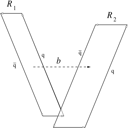
Figure 1: The scattering of two dipoles.

The four corners of the loops have the coordinates

$$C_{1} : (-T,-T,\vec{x}\,_{1}),(T,T,\vec{x}\,_{1}),(-T,-T,\vec{x^{\prime}}\,_{1}),(T,T,\vec{x^{\prime}}\,_{1})$$ (3)

$$C_{2} : (-T,T,\vec{x}\,_{2}),(T,-T,\vec{x}\,_{2}),(-T,T,\vec{x^{\prime}}\,_{2}),(T,-T,\vec{x^{\prime}}\,_{2})$$ (4)

where the arrow always indicates vectors in transverse space and $T$ goes to infinity.

The relative and centre coordinates are introduced as

$$\vec{R_{i}}=\vec{x}\,_{i}-\vec{x^{\prime}}\,_{i};\quad\vec{X}_{i}=\vec{x^{\prime}}\,_{i}+z_{i}\vec{R}_{i}~{}.$$ (5)

The vector $\vec{R}_{i}$ denotes the transverse extension of the loop $i$ and the quantity $z_{i}$ with $0\leq z_{i}\leq 1$ will later be identified with the longitudinal momentum fraction of the quark. The impact parameter vector $\vec{b}$ is defined by

$$\vec{b}=\vec{X}_{1}-\vec{X_{2}}~{}.$$ (6)

With this definition the $t$-dependent scattering amplitude can be obtained as the two-dimensional Fourier transform with respect to the impact parameter DGKP97 .

The basic element of the scattering matrix for colour-singlet quark-antiquark dipoles is the expectation value of two loops,

$$S(\vec{b},\vec{R}_{1},z_{1},\vec{R}_{2},z_{2}))=\frac{\textstyle{\frac{1}{9}}\langle W[C_{1}]W[C_{2}]\rangle}{\textstyle{\frac{1}{3}}\langle W[C_{1}]\rangle\textstyle{\frac{1}{3}}\langle W[C_{2}]\rangle}~{},$$ (7)

with

$$W[C_{i}]={\rm tr~{}P}\exp[-ig\oint_{{\cal S}_{i}}\mbox{\bf B}dx]$$ (8)

where ${\cal S}_{i}$ the border line of loop $i$.

We will discuss later how we pass from the dipole-dipole amplitudes to hadronic scattering (or photoproduction) amplitudes by integrating over light-cone wave functions.

The expectation value of the loops is approximately calculated using an extension of the stochastic vacuum model (SVM). In this model it is assumed that the long-distance behaviour of QCD can be approximated by a Gaussian stochastic process with the gluon field strength as the stochastic variable. This model yields confinement in non-Abelian gauge theories and is in conformity with the Mandelstam-t’Hooft  Man76 ; tHo76 picture of string formation through monopole condensation; we refer to DSS00 for a detailed review. In order to apply the model for the evaluation of two loops it has to be extended, since in a stochastic process with non-commuting variables the higher cumulants which must vanish in a Gaussian process are not uniquely defined.

In order to pass from the gluon potential occuring in the line integrals in Eq. (8) to the gluon field strength we have to apply the non-Abelian Stokes theorem. This implies a special choice of a surface containing both loops as borders. This choice is not unique, and in this paper we use one proposed in DFK94 ; for other possible choices, see SSP02 .

The general form of the basic correlator which determines the full Gaussian process is in our approach given by DS88

$$\langle:g^{2}F^{a}_{\mu\nu}(x)\Big{(}e^{-ig\int_{x}^{x^{\prime}}Adz}\Big{)}^{bc}\ F^{d}_{\rho\sigma}(x^{\prime}):\rangle=$$

$$~{}~{}~{}{\textstyle{{1}\over{96}}}\delta^{ab}\delta^{cd}\langle g^{2}FF\rangle_{B}\int{d^{4}k\over(2\pi)^{4}}\ e^{-ik.{(x-x^{\prime})}}\Big{(}(g_{\mu\rho}g_{\nu\sigma}-g_{\mu\sigma}g_{\nu\rho})\ \kappa~{}i\widetilde{D}(k^{2})$$

$$~{}~{}+(-g_{\nu\sigma}k_{\mu}k_{\rho}+g_{\nu\rho}k_{\mu}k_{\sigma}-g_{\mu\rho}k_{\nu}k_{\sigma}+g_{\mu\sigma}k_{\nu}k_{\rho})(1-\kappa)\ i\frac{d\widetilde{D}_{1}(k^{2})}{dk^{2}}\Big{)}~{}.$$

For the correlation functions we take the form proposed in DFK94

$$\tilde{D}(k^{2}) = \frac{27\pi^{4}k^{2}}{4a^{2}(k^{2}+\frac{9\pi^{2}}{64a^{2}})^{4}}~{},$$

$$\tilde{D}_{1}(k^{2}) = \frac{9\pi^{4}}{2a^{2}(k^{2}+\frac{9\pi^{2}}{64a^{2}})^{3}}~{},$$ (10)

with the parameters

$$a=0.346~{}{\rm fm}~{},\qquad\langle g^{2}FF\rangle a^{4}=23.5~{},\qquad\kappa=0.74~{},$$ (11)

where $a$ is the correlation length, which are in agreement with lattice results DGM99 ; Meg99 . This same parameter set has been used for many applications of the model to hadron-hadron, photon-hadron and photon-photon high energy interactions and will be used throughout this paper.

The formalism set up above allows us to calculate the scattering matrix in terms of the correlator (LABEL:msvc) using the assumptions of the stochastic-vacuum model. The most straightforward way is to expand the exponentials occuring in the Wegner-Wilson loops of Eq. (7). We then obtain

$$S(\vec{b},1,2) = {\textstyle\frac{1}{144}}{\rm tr}(\lambda^{a}\lambda^{b}){\rm tr}(\lambda^{c}\lambda^{d})$$ (12)

$$\times\Big{\langle}\int_{{\cal S}_{1}}d\sigma^{\mu\nu}F^{a}_{\mu\nu}\,\int_{{\cal S}_{2}}d\sigma^{\kappa\lambda}F^{c}_{\kappa\lambda}\int_{{\cal S}_{1}}d\sigma^{\mu\nu}F^{b}_{\mu\nu}\,\int_{{\cal S}_{2}}d\sigma^{\kappa\lambda}F^{d}_{\kappa\lambda}\Big{\rangle}_{B}$$

$$+\dots$$

where the dots represent products of more than four field-strength tensors and 1,2 stands for $\vec{R}_{1},z_{1},\vec{R}_{2},z_{2}$. Inserting the expressions (10) and performing the surface integrals we are finally lead to

$$S(\vec{b},1,2)=1-{\textstyle{{1}\over{9}}}\chi^{2}(\vec{b},1,2)~{},$$ (13)

with

$$\chi(\vec{b},1,2) = \frac{1}{96}\langle g^{2}FF\rangle\Big{(}I(\vec{x}_{1},\vec{x}_{2})+I(\vec{x}^{\prime}_{1},\vec{x}^{\prime}_{2})$$ (14)

$$~{}~{}~{}~{}~{}~{}~{}~{}-I(\vec{x}_{1},\vec{x}^{\prime}_{2})-I(\vec{x}^{\prime}_{1},\vec{x}_{2})\Big{)}.$$

Using the special form of the correlators in Eq. (10) we obtain

$$I(\vec{x}_{1},\vec{x}_{2}) = {\textstyle\frac{1}{2}}\pi\kappa\int_{0}^{1}dv\Big{(}|v\vec{x}_{2}-\vec{x}_{1}|^{2}K_{2}(\lambda^{-1}|v\vec{r}_{2}-\vec{x}_{1}|)~{}~{}~{}~{}~{}~{}~{}~{}~{}~{}~{}~{}$$ (15)

$$~{}~{}~{}~{}~{}~{}~{}~{}~{}~{}~{}~{}~{}~{}+|\vec{x}_{2}-v\vec{x}_{1}|^{2}K_{2}(\lambda^{-1}|\vec{x}_{2}-v\vec{x}_{1}|)\Big{)}$$

$$+(1-\kappa)\pi\lambda^{2}|\vec{x}_{2}-\vec{x}_{1}|^{2}K_{3}(\lambda^{-1}|\vec{x}_{2}-\vec{x}_{1}|)$$

where $\lambda=(3\pi/8)a~{}$ , and $K_{2}$ and $K_{3}$ are modified Bessel functions.

A more refined method to treat the two traces has been developed by Berger and Nachtmann BN99 . The main idea is to interpret the product of the two separate traces in Eq. (12) over $3\times 3$ matrices (generators of $SU(3)$ in the fundamental representation) as one trace ${\rm Tr}_{2}$ in the product space of the two fundamental representations of $SU(3)$; that is ${\rm Tr}_{2}$ acts in $SU(3)\otimes SU(3)$. Thus

$$S(\vec{b},1,2) = \textstyle{\frac{1}{9}}{\rm Tr}_{2}\Big{\langle}\exp\Big{(}-ig\int_{{\cal S}_{1}}d\sigma^{\mu\nu}F^{a}_{\mu\nu}({\textstyle\frac{1}{2}}\lambda^{a}\otimes 1)\Big{)}$$ (16)

$$\times\exp\Big{(}-ig\int_{{\cal S}_{2}}d\sigma^{\mu\nu}F^{c}_{\mu\nu}(1\otimes{\textstyle\frac{1}{2}}\lambda^{c}\big{)}\Big{)}\Big{\rangle}_{B}~{}.$$

The two exponentials commute in the product space and we can write the right-hand side of this equation as a single exponential

$$S(\vec{b},1,2)=\textstyle{\frac{1}{9}}\,{\rm Tr}_{2}\Big{\langle}\exp\Big{(}-ig\int_{{\cal S}}d\sigma^{\mu\nu}\mbox{\bf F}_{\mu\nu}\Big{)}\Big{\rangle}_{B}~{},$$ (17)

where the surface integral extends over the surfaces ${\cal S}_{1}$ and ${\cal S}_{2}$, and $\mbox{\bf F}_{\mu\nu}$ takes its values in the product algebra of $SU(3)\otimes SU(3)$. We can now make a cluster expansion with stochastic variables from the product algebra and using the correlator (10) we finally obtains  BN99

$$S(\vec{b},1,2)=\textstyle{\frac{2}{3}}e^{-\frac{1}{3}i\chi}+\textstyle{\frac{1}{3}}e^{\frac{2}{3}i\chi}~{},$$ (18)

where $\chi=\chi(\vec{b},1,2)$ is the same as given in Eq. (14).

In the following we refer to the first method leading to Eq. (13) as the expansion method, and the second method leading to Eq. (18) as the matrix-cumulant method.

In a very loose sense we can consider the quantity $\chi$ as representing the exchange of a nonperturbative gluon. In this sense the expansion method takes only into account the exchange of two nonperturbative gluons. The matrix cumulant method then takes also into account multiple gluon exchange; it will automatically satisfy unitarity constraints for hadronic cross sections. An expansion of Eq. (18) in $\chi$ yields in leading order the result obtained in Eq. (13) above, namely

$$S(\vec{b},1,2)=1-\textstyle{\frac{1}{9}}\chi^{2}-\dots$$ (19)

We also consider the eikonal unitarisation method

$$S(\vec{b},1,2)=e^{-\chi^{2}/9}~{},$$ (20)

which is similar to forms used to study saturation effects pqcd4 ; CFKS01 . Like the matrix-cumulant method it corresponds to multiple exchange, but here the exchanged objects represented by $\chi$ are coupled in such a way that always a pair forms a color singlet whereas in the matrix-cumulant method only the entirety of the exchanged objects has to form a colour singlet. The three different methods are illustrated in Fig. 2   .

Figure 2: Illustration of a) the expansion metod, b) the matrix-cumulant method and c) the eikonal method. The gluon line with a $\chi$ corresponds to the expression (14) and can be viewed loosely as the exchange of a nonperturbative gluon.

The matrix element for dipole-dipole scattering with momentum transfer $\vec{q}$ is then given by

$$T_{fi}(s,t,\vec{R}_{1},z_{1},\vec{R}_{2},z_{2})=-2is\int d^{2}b\,e^{i\vec{q}.\vec{b}}\Big{(}S(\vec{b},1,2)-1\Big{)}~{},$$ (21)

with $t=-\vec{q}^{2}$.

The treatment of three quarks in a colour-singlet state is analogous to the scattering of two dipoles, but technically more involved. We refer to the literature DFK94 ; BN99 for the corresponding results.

If the parameters of the stochastic-vacuum model are taken to be independent of the energy, the resulting cross sections turn out to be independent of the scattering energy too. The observed energy dependence has therefore to be introduced by hand. One way is to make the size of the hadrons energy dependent  DFK94 ; FP97 . This has been shown to be very simple and effective for purely hadronic processes. We here adopt the two-Pomeron approach of Donnachie and Landshoff DL98 , coupling a soft Pomeron with intercept 1.08 to large and a hard Pomeron with intercept 1.42 to small dipoles DDR00 ; DD02 .

Specifically we introduce an energy dependence of the quantity $\chi$, Eq. (14)

$$\chi(b,1,2) \to \chi^{E}(b,1,2,s)=\chi(b,1,2)\Bigg{(}\frac{s}{s_{0}}\Bigg{)}^{\epsilon_{s}/2}\mbox{ for }R_{1}\mbox{ and }R_{2}>r_{c}$$

$$\chi(b,1,2) \to \chi^{E}(b,1,2,s)=\chi(b,1,2)\Bigg{(}\frac{sR_{i}^{2}}{s_{0}r_{c}^{2}}\Bigg{)}^{\epsilon_{h}/2}\mbox{ for }R_{i}\leq r_{c},i=1\mbox{ or }2$$

$$\chi(b,1,2) \to \chi^{E}(b,1,2,s)=\chi(b,1,2)\Bigg{(}\frac{sR_{1}R_{2}}{s_{0}r_{c}^{2}}\Bigg{)}^{\epsilon_{h}/2}\mbox{ for }R_{1}~{}\mbox{\bf{ and }}~{}R_{2}\leq r_{c}$$

with $\epsilon_{s}=0.08,~{}\epsilon_{h}=0.42$ taken from DL98 and $r_{c}$=0.22 fm taken from a treatment of the proton structure function DD02 .

II.2 Wave functions and hadronic reactions

We are interested in reaction amplitudes where the external particles are physical hadrons and photons. We obtain such amplitudes from the dipole-dipole scattering amplitude (21) by integrating over all dipoles sizes with the light-cone wave functions of the participating particles as weights.

A meson or a photon is here described by a light-cone wave function $\psi_{n}(\vec{R}_{i},z_{i})$ of a quark and an antiquark with relative transverse coordinates $\vec{R}_{i}$ and quark longitudinal momentum fraction $z_{i}$. The meson or photon scattering amplitude for the reaction $a~{}b\to c~{}d$ is then obtained from the dipole-dipole scattering amplitude $T_{fi}(s,t,\vec{R}_{1},z_{1},\vec{R}_{2},z_{2})$ of Eq. (21) by

$$T_{ab\to cd}(s,t)=-2is\int d^{2}\vec{b}\,e^{i\vec{p}.\vec{b}}\Big{(}S_{ab\to cd}(\vec{b},s)-1\Big{)}~{},$$ (23)

where

$$S_{ab\to cd}(\vec{b},s) = \int d^{2}R_{1}\int d^{2}R_{2}\int_{0}^{1}dz_{1}\int_{0}^{1}dz_{2}~{}\psi_{c}^{*}(\vec{R}_{1},z_{1})\psi_{a}(\vec{R}_{1},z_{1})$$ (24)

$$\times~{}\psi_{d}^{*}(\vec{R}_{2},z_{2})\psi_{b}(\vec{R}_{2},z_{2})S(\vec{b},1,2)~{}.$$

The normalization is such that

$$\frac{d\sigma}{d|t|}=\frac{1}{16\pi~{}s^{2}}~{}|T_{ab\to cd}(s,t)|^{2}~{}.$$ (25)

For the heavy quark content of a photon the perturbative expressions for the wave functions are reliable since the charm quark mass sets the scale. Although we need in the present work only with the transverse wave function, we give for completeness the expressions for both transverse and longitudinal photons, the latter being needed for electroproduction of mesons. For photons of helicities 1, -1 and 0, we write respectively

$$\psi_{\gamma,1}(Q^{2};z,r,\theta)=$$ (26)

$$\hat{e}_{f}\frac{\sqrt{6\alpha}}{2\pi}\Big{[}i\epsilon e^{i\theta}(z\delta_{h,+}\delta_{\bar{h},-}-\bar{z}\delta_{h,-}\delta_{\bar{h},+})K_{1}(\epsilon r)+m_{f}\delta_{h,+}\delta_{\bar{h},+}K_{0}(\epsilon r)\Big{]}~{},$$

$$\psi_{\gamma,-1}(Q^{2};z,r,\theta)=$$ (27)

$$\hat{e}_{f}\frac{\sqrt{6\alpha}}{2\pi}\Big{[}i\epsilon e^{-i\theta}(\bar{z}\delta_{h,+}\delta_{\bar{h},-}-z\delta_{h,-}\delta_{\bar{h},+})K_{1}(\epsilon r)+m_{f}\delta_{h,-}\delta_{\bar{h},-}K_{0}(\epsilon r)\Big{]}$$

and

$$\psi_{\gamma,0}(Q^{2};z,r)=\hat{e}_{q}\frac{\sqrt{3\alpha}}{2\pi}(-2z\bar{z})~{}\delta_{h,-\bar{h}}~{}Q~{}K_{0}(\epsilon r)~{},$$ (28)

where

$$\epsilon=\sqrt{z\bar{z}Q^{2}+m_{f}^{2}}~{},$$ (29)

and $m_{f}$ is the quark mass and $\hat{e}_{f}$ is the quark charge in units of the elementary charge for each flavour $f$; $K_{0}$, $K_{1}$ are the modified Bessel functions.

Meson wave functions are more model dependent than photon wave functions and especially the spin structure can be quite complicated BB98 . In this paper we take for the vector mesons the spin structure from the vector current leading to similar expressions as for the photon DGKP97 , namely

$$\psi_{V,+1}(z,r) = \phi_{V}(z,r)\Big{(}i\omega^{2}re^{i\theta}(z\delta_{h,+}\delta_{\bar{h},-}-\bar{z}\delta_{h,-}\delta_{\bar{h},+})+m_{f}\delta_{h,+}\delta_{\bar{h},+}\Big{)}~{},$$

$$\psi_{V,-1}(z,r) = \phi_{V}(z,r)\Big{(}i\omega^{2}re^{-i\theta}(\bar{z}\delta_{h,+}\delta_{\bar{h},-}-z\delta_{h,-}\delta_{\bar{h},+})+m_{f}\delta_{h,-}\delta_{\bar{h},-}\Big{)}$$ (30)

and

$$\psi_{V,0}(z,r)=\phi(z,r)_{V}\Big{(}\omega 4z\bar{z}\delta_{h,-\bar{h}}\Big{)}~{}.$$ (31)

Here $\pm 1$ and $0$ denote transverse and longitudinal polarizations of the vector meson, and $h$ and $\bar{h}$ represent the helicities of quark and antiquark respectively.

The functions $\phi_{V}(z,r)$ are constrained by the normalisation condition and by the electromagnetic decay width, as described in the Appendix. Making for the $r$ dependence a Gaussian ansatz, the parameters are then completely determined by the two conditions just mentioned. For the $z$ dependence we make two ansätze: one is suggested by the phenomenologically very successfull Bauer-Stech-Wirbel model BSW87

$$\phi_{\rm BSW}(z,r)=\frac{N}{\sqrt{4\pi~{}}}~{}\sqrt{z(1-z)~{}}~{}\exp\Big{[}-\frac{M_{V}^{2}}{2\omega^{2}}(z-\frac{1}{2})^{2}\Big{]}~{}~{}\exp[-\frac{1}{2}\omega^{2}r^{2}]~{}.$$ (32)

The other choice is obtained in the spirit of Brodsky-Lepage BL80 from a non-relativistic wave function in the rest frame where the transition to the light-cone coordinates is achieved by the replacement of the relative momentum $\vec{k}$ of the two constituents by the transverse momentum $\vec{k}_{T}$ and the longitudinal momentum fraction of the quark according to

$$k^{2}\to\frac{k_{T}^{2}+m_{f}^{2}}{4z(1-z)}-m_{f}^{2}~{}.$$ (33)

This procedure only makes sense for a finite quark mass and leads to a more photon-like $z$ dependence of the wave function. We then write

$$\phi_{\rm BL}(z,r)=\frac{N}{\sqrt{4\pi~{}}}\exp\Big{[}-\frac{m_{f}^{2}(z-\frac{1}{2})^{2}}{2\omega^{2}z(1-z)}\Big{]}~{}\exp[-2z(1-z)\omega^{2}r^{2}]~{}.$$ (34)

$M_{V}$ and $m_{f}$ represent respectively the vector meson mass and the the quark mass.

For the proton we should use a three quark wave function which in principle poses no problems DFK94 . Earlier investigations have shown however that a quark diquark structure of the proton leads to phenomenologically consistent results and most applications have been made in this picture. The quark-diquark nucleon wave function can be treated like a quark-antiquark meson wave function and again we make a Gaussian ansatz for the wave function and fix the longitudinal momentum fraction at $z\approx 1/2$  , namely

$$\psi_{p}(R)=\frac{1}{2\pi}\frac{1}{S_{p}}e^{-r^{2}/(2S_{p})^{2}}~{}.$$ (35)

The transverse size parameter $S_{p}$ of the proton is choosen to be

$$S_{p}=0.74~{}~{}~{}{\rm fm}~{},$$ (36)

which leads to a good description of $pp$ scattering and also to a good proton form factor DNPW01 .

For the charm mass we adopt the value used in a previous analysis of structure functions DD02 ,

$$m_{c}=1.25~{}\rm{GeV}~{}.$$ (37)

This value lies in the middle of the range of masses of the modified minimal subtraction scheme PDG02 . The dependence of the charm mass is discussed in the Appendix.

This finishes the description of the general model, with characterization of all parameters. It should be noted that in the original application of the matrix cumulant method BN99 a slightly different set of parameters was used in order to get an optimal overall description of the elastic proton-proton cross section. Showing in the present paper the values of amplitudes and cross sections evaluated with only one set of parameters we wish to emphasize the magnitude of the influence of multiple scattering mechanisms.

II.3 Photoproduction of vector mesons

Using the results of the two previous sub-sections we can calculate the scattering amplitudes for photoproduction of vector mesons.

Inserting the wave functions of Eqs.(27),(30) and (35) into the production amplitude (24) we obtain

$$S_{\gamma p\to Vp}(b)=\int d^{2}R_{1}~{}\int dz_{1}\,\int d^{2}R_{2}\,\rho_{\gamma,V,\lambda}(z_{1},R_{1})|\psi_{p}(R_{2})|^{2}S(b,z_{1},\vec{R}_{1},1/2,\vec{R}_{2})~{},$$ (38)

where $\rho_{\gamma,V,\lambda}(z_{1},R_{1})$ is the photon-vector-meson overlap function

$$\rho_{\gamma,V,\lambda}(z_{1},R_{1}) = \hat{e}_{q}\frac{\sqrt{6\alpha}}{2\pi}~{}~{}\phi_{BSW/BL}(z,R_{1})$$ (39)

$$\times \Big{(}\epsilon~{}\omega^{2}R_{1}\big{[}z^{2}+(1-z)^{2}\big{]}K_{1}(m_{f}~{}R_{1})+m_{f}^{2}K_{0}(m_{f}~{}R_{1})\Big{)}~{}.$$

The overlap densities are independent of the angles $\theta_{1}$ and $\theta_{2}$ of $\vec{R}_{1}$ and $\vec{R}_{2}$, and the functions $\chi(\vec{b},1,2)$ change sign if $\vec{R}_{1}$ or $\vec{R}_{2}$ is reversed, as can be seen easily from Eq. (14) by noting that $\vec{R}_{i}\to-\vec{R}_{i}$ corresponds to $(\vec{x}_{i},\vec{x}^{\prime}_{i})\to(\vec{x}^{\prime}_{i},\vec{x}_{i})$. Inserting the result (18) of the matrix cumulant method into Eq. (38) we see that after integration over the angles $\theta_{1}$ and $\theta_{2}$ only the even terms in $\chi$ survive and the exponentials in Eq. (18) can be replaced by cosines. Therefore we may insert in Eq. (38), as result of the matrix cumulant method,

$$S(\vec{b},1,2)=\textstyle{\frac{2}{3}}\cos\Big{(}\frac{1}{3}\chi\Big{)}+\textstyle{\frac{1}{3}}\cos\Big{(}\frac{2}{3}\chi\Big{)}\equiv 1+\frac{2}{3}\Big{[}\cos\Big{(}\frac{1}{3}\chi\Big{)}+2\Big{]}\Big{[}\cos\Big{(}\frac{1}{3}\chi\Big{)}-1\Big{]}$$ (40)

This form guarantees that the amplitude remains inside the unitarity bounds if $\chi$ becomes large. Differences with respect to the expansion method, Eq. (13), increase at high energies.

If the energy dependent expressions in Eq. (LABEL:chiE) are introduced it turns out that the hard part of the proton, $R_{1}\leq r_{c}$ gives for energies below the TeV region only a negligible contribution, so we have only to consider the two cases $R_{1}\leq r_{c}$ and $R_{1}>r_{c}$.

Now all formulae are set up and all parameters are fixed.

Our results for the differential and total cross section of $J/\psi$ photoproduction in the expansion method are written

$$\frac{d\sigma}{d|t|}=\bigg{(}A_{h}(t)\Big{(}\frac{s}{s_{0}}\Big{)}^{0.42}+A_{s}(t)\Big{(}\frac{s}{s_{0}}\Big{)}^{0.08}\bigg{)}^{2}~{}.$$ (41)

The soft and hard amplitudes for the case of the BSW wave function can be conveniently expressed by the parametrisations

$$A_{s}(t) = \frac{10.82\exp(-1.07|t|)}{1+3.39|t|}~{},$$

$$A_{h}(t) = \frac{2.0\exp(-0.94|t|)}{1+3.39|t|}~{},~{}(BSW)~{},$$ (42)

where $t$ is in GeV² and $A_{s,h}(t)$ in $\sqrt{\rm nb}/$GeV, $s_{0}=(20~{}{\rm GeV})^{2}$. For the case of the BL wave function the forms are very similar

$$A_{s}(t) = \frac{11.17\exp(-1.06|t|)}{1+3.26|t|}~{},$$

$$A_{h}(t) = \frac{2.1\exp(-0.95|t|)}{1+3.26|t|}~{},~{}(BL)~{}.$$ (43)

These very convenient parametrisations reproduce the exact results with an accuracy always better than 5 percent. We see that the t-dependence of the differential cross section predicted by our model is not a pure exponential, showing a curvature in a logarithimic scale. Since the parameters expressing the t-dependences of the hard and soft parts of the amplitude have rather similar values, the shape of the angular distribution (and the slope parameter) depend only weakly on the energy (we recall that we work with small values of $|t|$). The values of $A_{s}(t)$ and $A_{h}(t)$ are shown in Fig. (3), in solid line for the BWS and in dashed line for the BL wave function. These forms, together with Eq. (41) contain all results for the expansion method that will be used for comparison with experiments. At low energies the soft contribution is several times stronger than the hard one. The hard part reaches the soft part for $W$ about 240 GeV.

Since the differences between the two kinds of $J/\psi$ wave functions are very small, from now on in the present paper, we will use only one of them, namely the BSW wave function.

The results for the matrix cumulant method BN99 cannot be parametrized so easily, due to the nonlinear dependence of the amplitudes on the quantity $\chi^{E}(b,1,2,s)$, Eq. (LABEL:chiE). That is, we cannot factorize the $s$ and $t$ dependences of the soft and hard parts, as in Eq. (41). The same is true of the amplitudes obtained with the eikonal form of Eq. (20). In Fig. 3 we draw also the amplitudes for these two unitarization procedures, for a fixed energy $W=20$ GeV, where we see that the form of the t-dependence (in a limited $|t|$ interval) is not much affected by the saturation corrections. The same is true for higher energies.

Accurate parametrisations of the differential cross sections can be written in the form

$$\frac{d\sigma}{d|t|}=\frac{A\exp(-a|t|)}{1+b|t|}~{},$$ (44)

yielding results summarised in Tables 1, 2. We found that parametric forms with dipole factor like $1/(1+b|t|)^{2}$ do not lead to equally accurate representations for $d{\sigma}/d|t|$.

	exp.	matrix-cum.	eikonal
$W$	A	A	A
GeV	nb/GeV2	nb/GeV2	nb/GeV2
20	167.6	153.7	141.1
200	896.4	790.2	693.3
1000	5657	3983	3008

Table 1: Result for $A$ in the parametrisation (44) for the expansion, the matrix-cumulant and the eikonal methods.

	expansion		matrix-cumulant		eikonal
$W$	a	b	a	b	a	b
GeV	GeV-2	GeV-2	GeV-2	GeV-2	GeV-2	GeV-2
20	2.72	9.0	2.83	10	3.00	10
200	2.62	9.2	2.87	10	3.15	10
1000	2.56	9.3	3.38	10	3.78	10

Table 2: Results for parameters $a$ and $b$ (44) for the expansion, the matrix-cumulant and the eikonal methods at different energies.

Figure 3: $t$-dependence of soft and hard production amplitudes at the energy $W=\sqrt{s}=20$ GeV. The lines can be parametrised in forms $A(0)\exp(-a|t|)/(1+b|t|)$, as explained in the text. The solid and the dashed lines are the results for the expansion method Eq.(13), using respectively BSW and BL wave functions for $J/\psi$. The dotted line corresponds to the matrix-cumulant method Eq.(40) and the dot-dashed line to the eikonal method Eq.(20), both using BSW wave function.

Figure 4: Integrated elastic production $\gamma~{}p\to J/\psi~{}p$ cross section. In full line the result with the expansion method, Eq.(13). Dotted and dash-dotted lines correspond respectively to the matrix cumulant method of Eq. (40) and to the exponentiation form of Eq.(20). In the upper figure the same $\langle g^{2}FF\rangle a^{4}=23.5$ for the gluon condensate is used for the three curves. In the lower figure we show that the unitarization effects are compensated, in the present experimental range $\sqrt{s}\leq 300$ GeV, by slight changes of parameters: $\langle g^{2}FF\rangle a^{4}=$ 25.0 and 26.0 respectively for Eqs. (40) and (20). The behaviour at high energies is explained in the text.

For the integrated production cross section we obtain with the expansion procedure

$$\sigma=0.552\Big{(}\frac{s}{s_{0}}\Big{)}^{0.84}+13.539\Big{(}\frac{s}{s_{0}}\Big{)}^{0.16}+5.465\Big{(}\frac{s}{s_{0}}\Big{)}^{0.50}~{}.$$ (45)

In the upper part of Fig. 4 we show the results for the integrated cross sections using the same input-parameter set of Eqs. (11) and (36) for the expansion method of Eq. (13) and for the matrix cumulant expression of Eq. (40) and for the eikonal form of Eq. (20). The curves show the influence of possible multiple scattering corrections. In the lower part of Fig. 4 we instead choose slightly different values for the gluon condensate: $\langle g^{2}FF\rangle a^{4}=$ 25.0 and 26.0 respectively for Eqs. (40) and (20). This last figure shows that in the present experimental range, below 300 GeV, unitarity corrections are easily compensated by slight changes of one single parameter. Small changes in the value of the charm quark mass that enters in the wave function has important effects of the same kind.

We may conclude that these saturation effects are not clearly observed in elastic photoproduction of $J/\psi$ for energies up to 300 GeV.

It is interesting to investigate the behaviour of the integrated cross section at higher energies. While with the expansion method the cross section increase according to Eq. (45), in the unitarized cases the behaviour in the whole range $20\leq W\leq 1000$ GeV is described by the slower behaviour

$$\sigma(W)=\sigma(W_{0})\times[1+C\big{(}\frac{W}{W_{0}}\big{)}^{\delta}\log\big{(}\frac{W}{W_{0}}\big{)}]~{},$$ (46)

with $\delta$ = 0.7 for the matrix cumulant (dotted lines) cases and = 0.6 for the exponentiation procedure (dot-dashed lines). The values of the multiplicative constant C vary a little with the choice of $\langle g^{2}FF\rangle a^{4}=$ as follows: C=0.36 and 0.35 in the matrix cumulant method respectively for 23.5 and 25.0 , and C=0.43 and 0.41 in the exponentiation procedure respectively for gluon condensates 23.5 and 26.0.

If we restrict ourselves to the experimental energy range from 20 to 300 GeV, the results obtained with the expansion method can be represented with an effective power like form

$$\sigma(W)=14.6+9.37\big{(}\frac{W}{W_{0}}\big{)}^{1.08}~{}.$$ (47)

The functional integrals occuring in the basic expression (7) for the S-matrix are in our approach approximately evaluated with the help of the stochastic vacuum model. This model is an approximation appropriate only for the soft part of QCD. The higher the momentum transfer the more important will become contributions of hard gluons. Therefore we expect our calculations to be best at small momentum transfer. Of course we cannot predict the exact scale where hard scattering becomes important but investigations of the gluon distributions in hadrons and virtual photons SSDP02 indicate that the hard component becomes as important as the soft part at a transverse momentum of the gluons $|k_{T}|\approx 1$ GeV, so that a safe limit for soft process is $\sqrt{|t|}\ll 1$ GeV. We also expect that for photoproduction of $\Upsilon$-mesons even at small momentum transfer hard gluons play a more important role . There the small size of the $\Upsilon$ suppresses the contribution of the soft (nonperturbative) gluons as compared to the hard ones.

Another limitation of our approach is given by the WKB approximation underlying the nonperturbative approach Nac91 to scattering. Here the path is assumed to be the classical one, being nearly a straight line. This also determines the momentum transfer below which the model can be safely applied. The WKB approximation should be more reliable at high energies, and this restricts the application of the model to energies higher than $\sqrt{s}\approx 20$ GeV.

Apart from the approximations characteristic of the stochastic vacuum model, also the wave functions are treated in a very simplified form. From previous experience we expect the reliabillity of the model to be about 10 % in the amplitudes. Thus, putting all this together, discrepancies between theory and experiment below 20 % for the production cross sections could be considered as natural.

III Comparison with experiment

Figure 5: Forward differential cross section $\big{(}d\sigma/dt\big{)}(t=0)$ for the reaction $\gamma~{}p\to J/\psi~{}p$. The line represents our results with the expansion method. The experimental results are from the H1 Collaboration H1-00 for the momentum transfer in the interval $0\leq|t|=0.053$ GeV²

The experimental H1-00 forward production cross section $\big{(}d\sigma/dt\big{)}(t=0)$ is shown in Fig. 5. Only the H1 Collaboration measures directly this quantity, represented by their $0\leq|t|\leq 0.053$ GeV² bin . The values reported by Zeus Zeus02 correspond to the extrapolations to $|t|=0$ of their fitted straight lines, as will be discussed later (Fig. 8).

A direct comparison with both ZEUS and H1 data in the forward direction can be made at $|t|=0.1$ GeV², and this is presented in Fig. 6. Here we see a very satisfactory agreement between theory and ZEUS and H1 data, with a remarkable theoretical description of the energy dependence in the whole range from 40 to 260 GeV.

Figure 6: Differential cross section $\big{(}d\sigma/dt\big{)}(|t|=0.1)$ for the elastic production $\gamma~{}p\to J/\psi~{}p$ at $|t|=0.1$ GeV². The solid line represents our calculation with the expansion method. The experimental results are from ZEUS Zeus02 and H1 H1-00 collaborations. Zeus data are separately reported for observations of $J/\psi\to\mu^{+}\mu^{-}$ and $J/\psi\to e^{+}e^{-}$ decays.

Figure 7: Integrated cross section for the reaction $\gamma~{}p\to J/\psi~{}p$. The experimental data are from the H1 H1-00 and Zeus Zeus02 collaborations. The point marked with a star at $W=16.8$ GeV represents results from fixed target experiments target1 ; target2 ; target3 . The solid line is obtained with the expansion method. The dashed line shows our results using the matrix cumulant method, with the same set of parameters, as in the top part of Fig. 4. To show the influence of a different choice for the charm mass, the dot-dashed line gives the results obtained with the expansion method, using $m_{c}=$ 1.2 GeV.

The integrated production cross section is presented in Fig. 7, showing again a reasonable agreement of our model with all data up to nearly 300 GeV. The solid line corresponds to our calculation using the $\chi^{2}$ expansion of Eq. (13). As we have already shown in Fig. 4, the effects of saturation introduced by the matrix cumulant or exponentiation method are not very large, are within our expected errors, and can be compensated by slight change in parameters. In the figure the dashed line represents the results obtained with the matrix cumulant, using the standard set of parameters. We have shown in Fig. 4 that choosing $\langle g^{2}FF\rangle a^{4}=$ 25.0 , instead of 23.5, the result of the matrix-cumulant coincides in this energy range nearly with the solid line in Fig. 7. To show the influence of the value of the charm mass in the calculation, this figure includes also (dot-dashed line) the results obtained using a value $m_{c}=1.2$ GeV in the wave functions.

The H1 and ZEUS data on integrated elastic cross sections put together can be fitted by either of the two forms (in nb)

$$\sigma(W)=25.8~{}\big{(}\frac{W}{W_{0}}\big{)}^{0.71}~{},$$ (48)

or

$$\sigma(W)=26.0+17.14~{}\big{(}\frac{W}{W_{0}}\big{)}^{0.43}~{}\log\big{(}\frac{W}{W_{0}}\big{)}~{},$$ (49)

with the same deviation $\chi^{2}=1.73$ per degree of freedom.

In Fig. 8 we compare our calculations of differential cross sections with the most recent data from H1 and ZEUS experiments. The energy range is from 40 to 260 GeV, distributed in 9 bins, and the $|t|$ range is $(0-1.6)\rm{GeV}^{2}$. Where data from different experiments in similar energy bins are available, we plot them together in the same figure. We emphasize that our calculation contains no adjustable parameters and that these measurements cover a wide energy range.

Figure 8: $t$-dependence of differential cross sections for the reaction $\gamma~{}p\to J/\psi~{}p$. Data are from H1 H1-00 and ZEUS Zeus02 experiments. The solid curves represent our calculations, as described in the text. The dashed straight lines are Zeus fits in each of their energy bins.

As a quite general feature we see that for small values of the momentum transfer $t$ the agreement between experiment and theory is quite satifactory for all energies. For larger values of $|t|$ agreement with H1 data is still satisfactory, but at the lower and middle energies our results are in general below the new ZEUS data. At the highest energies, the agreement improves. Since in our model we take into account only nonperturbative effects it is not surprising that at larger momentum transfers where harder gluons are exchanged, some contributions are missing in our calculation. In FP02 a good fit up to $|t|\approx 6$ GeV² is indeed obtained.

Zeus gives exponential fits in $t$ to their data, which are indicated by dotted lines in our plots in Fig. (8) . From this fit the Zeus collaboration obtains the forward differential cross section and then evaluates the integrated elastic cross section. The plots show remarkable differences at $|t|=0$ between our results (with the epansion method) and the ZEUS extrapolated values obtained with a straight line.

As we have shown in the general description of the calculation, the differences between the expansion method and the matrix cumulant and exponentiation methods are not very large and could be absorbed in a slightly different choice of parameters. We do not include the corresponding lines in Fig. 8 in order not to overload the plots.

The data presented above are the most recent HERA data on $J/\psi$ photoproduction. Some of the pioneering fixed target experiments of 20 years ago were made at energies near $\sqrt{s}=20$ GeV , which is at the border of the range appropriate for our calculations. We have included in Fig. 7 a point at about 16.8 GeV representing this experimental effort target1 ; target2 ; target3 , showing that it fits well in the sequence of higher energy data points. As a historical tribute, we show in Fig. 9 the $|t|$-dependence of the differential cross sections obtained in some of these experiments. In this figure we draw together our curves for the expansion method of Eq. (13) (solid line), for the matrix cumulant result of Berger and Nachtmann BN99 given by Eq. (40) and for the exponentiation procedure of Eq. (20).

Figure 9: $t$-dependence of differential cross sections for the reaction $\gamma~{}p\to J/\psi~{}p$ at the low energies of some fixed target experiments target1 ; target2 ; target3 . The solid, dashed and dotted lines represent our results using Eqs. (13), (40) and Eq. (20) respectively.

We have also applied the model to photoproduction of $\Upsilon~{}(1S)$ mesons. As expected the results of our calculation are below the central values of the experimental data from Zeus upsil1 and H1   H1-00 , but the large errors do not allow a definite conclusion about the need of other contributions. We find it nevertheless quite astonishing that the nonperturbative model seems to yield at least a substantial fraction of the cross section for such a hard process. Our results shown in Fig. 10 can be compared with perturbative calculations upsil2 , upsil3 of the same process. In upsil2 the LO calculation taking into account the skewed parton distrubution in some way obtains results on the lower edge of the error bars, while in upsil3 additional contributions lead to values just through the central values of the measurements.

Figure 10: Integrated cross section for the reaction $\gamma~{}p\to\Upsilon~{}p$. Solid : our result with $m_{b}=4.2$ GeV, dashed with $m_{b}=4.4$ GeV. Experimental points from Zeus   upsil1 and H1   H1-00

IV Summary and discussion

The main purpose of this paper is to investigate to what extent photoproduction of $J/\psi(1S)$ mesons can be described in a purely nonperturbative QCD model. The model has been tested before, and the parameters used in the present work have been taken from previous publications on different processes. They were determined mainly from results of QCD lattice calculations and hadronic properties. Our parameter free results are compared with the more recent experimental data obtained at HERA by the H1 H1-00 and Zeus Zeus02 collaborations. Comparison of the calculated values of the differential cross sections with the data in nearly forward directions is presented in Figs. 5 and 6. The values reported by Zeus at $|t|=0$ are not direct measurements, but rather extrapoled values from linear fits, as shown in Fig. 8. In our view, these linear extrapolations do not account for possible structure in the very forward direction, and may lead to underestimated values, so that Fig. 5 only shows the H1 data. At $|t|=0.1~{}{\rm GeV}^{2}$ both H1 and Zeus direct measurements exist, and Fig. 6 shows that the theoretical model gives excellent description of the magnitude and of the energy dependence at low $|t|$.

Fig. 8 shows that at larger $|t|$ our calculations agree well with the H1 measurements and are below the Zeus points for energies up to $W=120$ GeV. At the highest energies the agreement with Zeus data is good, except that our model predicts a curvature, with a rise in the very forward direction. A clarification of this point is very important, since many models can only calculate the forward scattering amplitude and the test of the corresponding theoretical ideas depend on this kind of experimental data. Our model leads to a peculiar form-factor dependence which is exhibited in Fig. 3 and represented by the parametrizations of Eqs. (41), (42) and (43). The t-dependence of the differential cross sections shows similar curvatures, represented by Eq. (44).

We recall that our model in meant to be tested in the low $|t|$ range, say below 1.0 GeV². For larger momentum transfers the differential cross section values are already 100 times smaller than in the soft region, and an additional genuinely hard contribution, however small (without influence on the integrated cross section), may play here an important role.

The integrated cross section is in reasonable agreement with the experimental data, as shown in Fig. 7.

We have studied particularly the influence of saturation. We have several methods based on the stochastic vacuum model to evaluate our model.

• The expansion method which corresponds loosely speaking to an exchange of two ,,nonperturbative” gluons.

• The matrix cumulant method BN99 which takes in some way multigluon exchange into account and respects the unitarity constraints for hadronic cross sections.

• The usual exponentiation of the profile function, as in Eq. (20).

The methods are illustrated in Fig. 2 and compared in Figs. 3 and 4. The energy dependence was introduced based on the two-pomeron model of Donnachie and Landshoff DL98 . In the expansion method it leads to a power like increase of the integrated cross section, while the matrix cumulant and in the exponentiation methods there is saturation due to the unitarity constraints on the dipole cross sections, inherently respected by the approach. Up to energies about 1000 GeV, the energy dependence in these unitarity controlled calculations is very well parametrized in forms given by Eq. (46). In Fig. 7 our calculations are compared with the data.

It should be noted that in photoproduction processes the Froissart theorem cannot be proved and that a powerlike increase does not contradict fundamental theorems of local quantum field theory.

At present energies and with present accuracies the data show no indication of saturation and are well compatible with the powerlike behaviour of the unconstrained two pomeron approach. But a comparison with the theoretical approaches that introduce saturation effects shows that these are also compatible with the experiment, considered some 20 % allowed variation in our model. Rather small changes of parameter values may account for differences among calculation procedures.

We have also tested two different types of wave functions and found only small differences in relevant results.

We conclude that, in the energy range available at HERA, the methods here studied yield results compatible with experiment. As can be seen from Fig. 4, sizeable deviations are only expected for energies above 300 GeV.

In our model the residues of both soft and hard pomerons are evaluated by nonperturbative methods but this seems to agree fairly well with the phenomenological value. This has already been noted in DD01 for a large number of total cross sections and forward amplitudes.

We have extended the use of our model to photoproduction of $\Upsilon(1S)$ mesons and found that it can yield at least a sizeable part of this supposedly hard process.

*

Appendix A Conditions on wave functions

The two parameters in the wave functions of the vector mesons, $N$ ans $\omega$, are determined by the normalisation condition and the leptonic decay width.

The square of the wave functions (30,31) summed over internal helicities is given for the transverse case by

$$|\psi_{X,\pm 1}(z,r)|^{2}=|\phi_{X}(z,r)|^{2}\times\Big{(}\omega^{4}r^{2}\big{[}z^{2}+(1-z)^{2}\big{]}+m_{f}^{2}\Big{)}$$ (50)

and for the longitudinal case by

$$|\psi_{X,0}(z,r)|^{2}=2~{}|\phi_{X}(z,r)|^{2}\times(\omega 4z\bar{z})^{2}~{}.$$ (51)

where the $X$ in the index stands for BSW   BSW87 or BL   BL80 -type wave functions. It has to fulfil the normalisation condition

$$\int_{0}^{1}dz\int|\psi_{X,\lambda}(z,r)|^{2}d^{2}{\mathbf{r}}=1~{}.$$ (52)

The condition which relates the wave function with the e.m. decay width $f_{V}$ is, for the transverse cases,

$$f_{V}=\hat{e}_{V}\frac{\sqrt{6~{}}}{M_{V}}\frac{\sqrt{4\pi~{}}}{16\pi^{3}}~{}\int_{0}^{1}dz\int d^{2}{\mathbf{k}}\frac{1}{z(1-z)}\Big{(}\big{[}z^{2}+(1-z)^{2}\big{]}k^{2}+m_{f}^{2}\Big{)}\tilde{\phi}_{X}(z,k)$$ (53)

and for the longitudinal cases

$$f_{V}=\hat{e}_{V}\omega\sqrt{3~{}}\frac{\sqrt{4\pi~{}}}{16\pi^{3}}~{}\int_{0}^{1}dz\int d^{2}{\mathbf{k}}~{}16~{}z(1-z)~{}\tilde{\phi}_{X}(z,k)~{}.$$ (54)

where $\tilde{\phi}_{X}(z,k)$ is the Fourier transform of $\phi_{X}(z,r)$, defined through

$$\phi_{X}(z,r)=\int\frac{d^{2}{\mathbf{k}}}{4\pi^{2}}~{}\tilde{\phi}_{X}(z,k)~{}\exp[-i{\mathbf{k}}\cdot{\mathbf{r}}]~{},$$ (55)

and $\hat{e}_{f}$ is the quark charge in units of the elementary charge, that is $\hat{e}=2/3$ for the $J/\psi$ and -1/3 for the $\Upsilon$.

The decay constant $f_{V}$ is related to the e.m. decay width $\Gamma_{e^{+}e^{-}}$ through

$$f_{V}^{2}=\frac{3M_{V}\Gamma_{e^{+}e^{-}}}{4\pi\alpha^{2}}~{}.$$ (56)

		BSW			BL
Meson	$m_{f}$	$\omega$	$N$	$S$	$\omega$	$N$	$S$
	[GeV]	[GeV]		[fm]	[GeV]		[fm]
$J/\psi(1S)$	$1.2$	$0.59$	$3.30$	$0.35$	$0.64$	$1.47$	$0.36$
	$1.25$	$0.58$	$3.17$	$0.36$	$0.63$	$1.44$	$0.35$
	$1.3$	$0.57$	$3.04$	$0.36$	$0.62$	$1.41$	$0.35$
$\Upsilon(1S)$	$4.2$	$1.29$	$2.48$	$0.16$	$1.32$	$1.17$	$0.16$
	$4.4$	$1.26$	$2.35$	$0.16$	$1.30$	$1.14$	$0.16$

Table 3: Values of $\omega$ , $N$ and size parameter $S$ for transverse wave functions of $J/\psi$ and $\Upsilon$ mesons.

In Table 3 we give the values of $N,~{}\omega$ and the mean square transverse radius for the $J/\psi$ and the $\Upsilon$ wave functions for different choices of the charm and bottom masses for the transverse BSW- and BL-type meson wave functions.

The $\gamma^{*}$-vector meson overlap functions, necessary for the calculation of photo- and electroproduction of vector mesons are obtained from Eqs. (30,31) and (27, 28), and are given by

a) transverse

$$\rho_{\gamma^{*}V,1}(z,r) = \hat{e}_{V}\frac{\sqrt{6\alpha}}{2\pi}~{}~{}\phi_{X}(z,r)$$ (57)

$$\times \Big{(}\epsilon~{}\omega^{2}r\big{[}z^{2}+(1-z)^{2}\big{]}K_{1}(\epsilon~{}r)+m_{f}^{2}K_{0}(\epsilon~{}r)\Big{)}=\hat{e}_{V}~{}\hat{\rho}_{\gamma V,1}(z,r)$$

b)longitudinal

$$\rho_{\gamma^{*}V,0}(z,r)=-16\hat{e}_{V}\frac{\sqrt{3\alpha}}{2\pi}~{}\omega~{}\phi_{X}(z,r)z^{2}(1-z)^{2}~{}Q~{}K_{0}(\epsilon~{}r)=\hat{e}_{V}~{}\hat{\rho}_{\gamma V,0}(z,r)~{},$$ (58)

where $\epsilon=\sqrt{z\bar{z}Q^{2}+m_{f}^{2}}$   .

The real photon-vector meson overlap is obtained by setting $Q=0$, i.e. the longitudinal part vanishes and $\epsilon\to m_{f}$.

The integrals of the square radius over the overlap functions

$$C(\lambda)=\int_{0}^{1}dz\int d^{2}{\mathbf{r}}~{}r^{2}~{}\rho_{\gamma V,\lambda}(z,r)~{}.$$ (59)

give an estimate of the effective strength for the production process, the square of these quantities being nearly proportional to the integrated cross sections. Thus the numbers in Table 4 tell us that the ratio between $\Upsilon$ and $J/\psi$ production cross sections at 20 GeV is about $10^{-3}$.

		BSW	BL
Meson	$m_{f}$	$C(\lambda=\pm 1)$	$C(\lambda=\pm 1)$
	[GeV]	[GeV-2]	[GeV-2]
$J/\psi(1S)$	$1.2$	$0.0103$	$0.0113$
	$1.25$	$0.0095$	$0.0102$
	$1.3$	$0.0088$	$0.0093$
$\Upsilon(1S)$	$4.2$	$-0.00034$	$-0.00035$
	$4.4$	$-0.00030$	$-0.00031$

Table 4: Values of the integrated square radius over the overlap functions, defined by Eq. (59), for the two kinds of transverse wave function.

References

- (1) M.G. Ryskin, Z. Phys. C 57 (1993) 89.
- (2) S.J. Brodsky et al., Phys. Rev. D 50 (1994) 3134.
- (3) M.G. Ryskin, R.G. Roberts, A.D. Martin, E.M. Levin, Z. Phys. C 76 (1997) 231.
- (4) E. Gotsman, E. Ferreira, E. Levin, U. Maor and E. Naftali, Phys. Lett. B 503 (2001) 277.
- (5) E. Gotsman, E. Levin, U. Maor and E. Naftali, Phys. Lett. B 532 (2002) 37.
- (6) O. Nachtmann, Annals Phys. 209 (1991) 436.
- (7) H. G. Dosch, Phys. Lett. B 190 (1987) 177.
- (8) H. G. Dosch and Y. A. Simonov, Phys. Lett. B 205 (1988) 339.
- (9) H.G. Dosch, E. Ferreira and A. Kramer, Phys. Rev. D 50 (1994) 1992
- (10) O. Nachtmann, Lectures at Schladming School 1996, arXiv:hep-ph/9609365.
- (11) H. G. Dosch, “Nonperturbative Methods in QCD”, in Hadron Physics 96, Ed. E. Ferreira et al., World Scientific, Singapore 1997
- (12) H. G. Dosch, Acta Phys. Polon. B 30 (1999) 3813.
- (13) H. G. Dosch, T. Gousset, G. Kulzinger and H. J. Pirner, Phys. Rev. D 55 (1997) 2602
- (14) S. Mandelstam, Phys. Rep. 23C (1976) 245
- (15) G. ’tHooft, in “High Energy Physics”, Ed. Zichichi, Bologna 1976
- (16) H. G. Dosch, V. I. Shevchenko and Y. A. Simonov, Phys. Rep. 372 (2002) 319 arXiv:hep-ph/0007223.
- (17) A. I. Shoshi, F. D. Steffen and H. J. Pirner, Nucl. Phys. A709(2002) 131
- (18) M. D’Elia, A. Di Giacomo and E. Meggiolaro, Nucl. Phys. Proc. Suppl. 73 (1999) 515 [arXiv:hep-lat/9811017].
- (19) E. Meggiolaro, Phys. Lett. B 451 (1999) 414 [arXiv:hep-ph/9807567].
- (20) E. R. Berger and O. Nachtmann, Eur. Phys. J. C 7 (1999) 459 [arXiv:hep-ph/9808320].
- (21) A. Capella, E. G. Ferreiro, A. Kaidalov and C. A. Salgado, IX Blois conference, Pruhonice 2001, Elastic and diffractive scattering
- (22) E. Ferreira and F. Pereira, Phys. Rev. D 56 (1997) 179 [arXiv:hep-ph/9705278].
- (23) A. Donnachie and P. V. Landshoff, Phys. Lett. B 437 (1998) 408 [arXiv:hep-ph/9806344].
- (24) A. Donnachie, H. G. Dosch and M. Rueter, Eur. Phys. J. C 13 (2000) 141 [arXiv:hep-ph/9908413].
- (25) A. Donnachie and H. G. Dosch, Phys. Rev. D 65 (2002) 014019 [arXiv:hep-ph/0106169].
- (26) P. Ball and V. M. Braun, Workshop on Continuous Advances in QCD, Minneapolis 1998 arXiv:hep-ph/9808229.
- (27) M. Bauer, B. Stech and M. Wirbel, Z. Phys. C 34 (1987) 103.
- (28) G. P. Lepage and S. J. Brodsky, Phys. Rev. D 22 (1980) 2157.
- (29) H. G. Dosch, O. Nachtmann, T. Paulus and S. Weinstock, Eur. Phys. J. C 21 (2001) 339 [arXiv:hep-ph/0012367].
- (30) K. Hagiwara et al. [Particle Data Group Collaboration], Phys. Rev. D 66 (2002) 010001.
- (31) A. I. Shoshi, F. D. Steffen, H. G. Dosch and H. J. Pirner, Phys. Rev. D66: 094019 (2002) arXiv:hep-ph/0207287.
- (32) C. Adloff et al., H1 Coll. Phys. Lett. B 483 (2000) 23
- (33) S. Chekanov et al., Zeus Coll. Eur. Phys. J. C 24 (2002) 345
- (34) J. R. Forshaw and G. Poludniowski, arXiv:hep-ph/0107068.
- (35) M. Binkley et al., E-401 Coll., Phys. Rev. Lett. 48 (1982) 73
- (36) M. Arneodo et al. (NMC Coll.) Phys. Lett. B 332 (1994) 195
- (37) J. J. Aubert (EMC Coll.) Nucl. Phys. B 213 (1983) 1
- (38) J. Breitweg et al., Zeus Coll., Phys. Lett. B 437 (1998) 432
- (39) L. Frankfurt, M. McDermont and M. Strikman, JHEP 02 (1999) 002
- (40) A.D. Martin, M.G. Ryskin and T. Teubner, Phys. Lett. B 454 (1999) 348
- (41) A. Donnachie and H. G. Dosch, Phys. Lett. B 502 (2001) 74 [arXiv:hep-ph/0010227].