Neutrino Mass, Proton Decay and Dark Matter in TeV Scale Universal Extra Dimension Models

Abstract

We show how the problem of small neutrino masses and suppressed proton decay can be simultaneously resolved in 6-D universal extra dimension models (UED) with a low fundamental scale using extended gauge groups that contain the local $B-L$ symmetry. The extra space dimensions are compactified either on a $T^{2}/Z_{2}$ or $T^{2}/Z_{2}\times Z^{\prime}_{2}$ orbifold depending on whether the full gauge group is $SU(2)_{L}\times U(1)_{I_{3R}}\times U(1)_{B-L}$ or $SU(2)_{L}\times SU(2)_{R}\times U(1)_{B-L}$. In both cases, neutrino masses are suppressed by an appropriate orbifold parity assignment for the standard model singlet neutrinos and the proton decay rate is suppressed due to a residual discrete symmetry left over from compactification. For lower values of the fundamental scale, a dominant decay mode of the neutron is $n\rightarrow 3\nu$. An interesting consequence of the model is a possible two component picture for dark matter of the universe.

I Introduction

The possibility that the fundamental scale of nature ($M_{*}$) is in the multi-TeV range has been the focus of great deal of activity in the past several years [1]. These models are inspired by results in nonperturbative string theories and may therefore be providing a possibility of testing string theories in colliders as well as other low energy measurements. Furthermore, they also provide a new way to look at the puzzles of the standard model such as the gauge hierarchy and fermion masses. Even regardless of these motivations, their sharp differences from the usual “grand” desert picture of beyond the standard model physics makes them interesting enough to pursue their phenomenological as well as cosmological implications. As it is well known the high value of the conventional Planck scale is a derived scale in these models and arises out of a combination of $M_{*}$ and the compactification sizes of the extra dimensions. When the sizes of the extra dimensions are large, many other phenomenological consequences ensue and have been widely discussed in literature.

Even though these models are attractive in many ways, they have two fundamental problems that need to be resolved before they can be taken seriously: (i) they provide no simple way to understand small neutrino masses since the familiar seesaw mechanism[2] requires scales of order $10^{12}$ GeV or so, which are much higher than $M_{*}$; and (ii) no simple way to suppress proton decay induced by physics at the string scale.

A proposal for solving the neutrino mass problem using a singlet neutrino in the entire 5-dimensional bulk (so called bulk neutrinos) was proposed in ref. [3]. The smallness of neutrino masses in this picture owe their origin to large bulk radius rather than a large mass scale as in seesaw models. This new way of discussing neutrino masses has many new implications which have been studied in several papers [4]. In this case however, one has to assume the existence of a global B-L symmetry in the theory to prevent dangerous operators like $(LH)^{2}/M_{*}$ from destabilizing the neutrino masses. Since there is a general lore that there should be no global symmetries in string theories, barring the possibility that the global symmetry arises accidentally, we face a problem.

Proton decay in such models can arise due to the presence of nonrenormalizable operators of the form

$${QQQL\over M_{*}}~{};$$ (1)

which would clearly lead to an unacceptably short lifetime for the proton, many orders of magnitude below the present experimental lower limit.

In a recent paper [5] a solution to the proton decay problem was proposed in the context of the so called universal extra dimension models (UED) [6] where the number of space-time dimensions where all standard model (SM) fields reside is six and the fundamental scale of nature is in the TeV range. The main observation of [5] is that in six dimensional UED models, the extra space-time dimensions (the 5th and 6th dimensions) provide a new $U(1)$ symmetry under which the SM fermions are “charged” and enough of this symmetry survives the process of orbifold compactification that it suppresses proton decay to a very high degree. In the model of [5], the surviving symmetry is $Z_{8}$, so that the leading order baryon number violating operator has dimension 16 in six dimensions and thus highly suppressed.

No simple solution to the neutrino mass problem has been found in these models.

In a recent paper[7], a new way to solve the neutrino mass problem in TeV scale gravity models was proposed in higher dimensional theories without invoking the bulk neutrino or large extra dimensions. Instead, it was noted that in a 5-dimensional UED model based on an extended gauge symmetry $SU(2)_{L}\times SU(2)_{R}\times U(1)_{B-L}$ if the right handed neutrino is given a “twisted” orbifold boundary condition, the leading order neutrino mass operator has sufficiently high dimension so that its contribution to $m_{\nu}$ is suppressed despite the fundamental scale being low. The essential trick used is to project the familiar right handed neutrinos out of the zero mode spectrum of the theory. The main reasons that this solves the neutrino mass problem are as follows:

• (i) the local B-L symmetry forbids the operator $LHLH/M^{*}$;

• (ii) the assignment of the orbifold symmetry to the chiral components of the right handed neutrino $N$ forbids the conventional Dirac mass of the neutrinos.

The resulting lowest dimension operator contributing to the Majorana neutrino mass in five dimensions has dimension d=10 and there is a mini-seesaw for the Dirac mass leading to eV neutrino mass without any fine tuning. There was also no need to assume any global symmetries. A fundamental scale $M_{*}$ of 30-100 TeV and a compactification scale of order of a TeV was sufficient for phenomenological consistency as well as for giving small neutrino masses. It was speculated in this paper that when extended to six dimensions, the model also solves the proton decay problem.

In this paper, we first present a simpler six dimensional model based on the smaller gauge group $SU(2)_{L}\times U(1)_{I_{3R}}\times U(1)_{B-L}$ and a more economical fermion spectrum and show using $T^{2}/Z_{2}$ compactification that, we can solve both the neutrino mass and proton decay problems simultaneously. The compactification scale as well as the scale of $B-L$ breaking in this model are in the range of a TeV and the fundamental scale $M_{*}$ anywhere from 10-100 TeV. We then extend the gauge group to the left-right symmetric case and show how the same results are maintained; in this case however, we need to have the compactification on $T^{2}/Z_{2}\times Z^{\prime}_{2}$, which is very similar to our earlier work [7], now extended to six dimensions. Furthermore, we find some new decay modes for the nucleon in both models that may have lifetimes in the range of experimental accessibility. We then discuss the question of dark matter in these models.

In addition to solving the neutrino mass and proton decay problem, the models have the following interesting features:

• they predict the existence of a light $Z^{\prime}$ with mass at the compactification scale (of order of a TeV);

• they predict baryon number violating processes where both neutron and proton decay to final states with three leptons, e.g. $n\rightarrow\nu\bar{\nu}_{s}\bar{\nu}_{s}$;  $n\rightarrow\pi^{0}\nu_{e}\bar{\nu}_{s}\bar{\nu}_{s}$;  $n\rightarrow\pi^{+}e^{-}\bar{\nu}_{s}\bar{\nu}_{s}$;  and $p\rightarrow\pi^{+}\nu_{e}\bar{\nu}_{s}\bar{\nu}_{s}$.

• The model gives a two component picture of dark matter with $\gamma_{KK}$ and $\nu_{R}$ both playing the role of dark matter.

We organize our discussion as follows: in section II we present the $SU(2)_{L}\times U(1)_{I_{3R}}\times U(1)_{B-L}$ model and show how one solves the neutrino mass and proton decay problems using $T^{2}/Z_{2}$ compactification. In sec. III, we introduce the left-right extension of this model. In section IV, we discuss the anomaly cancellations conditions for both these models, which drive us to the conclusion that the model should contain at least three families. This provides a generalization of the results of Ref. [8] to the case of extended gauge groups. In section V, we discuss the $T^{2}/Z_{2}\times Z^{\prime}_{2}$ orbifolding of the two extra space-like dimensions, the breaking of the six dimensional Lorentz symmetries and the generalities for the mode expansion and mass spectrum of the theory. In section VI we introduce our $Z_{2}\times Z^{\prime}_{2}$ charge assignments for the particles of the model and discuss the orbifold and spontaneous symmetry breaking. The mass pectrum and a brief discussion of phenomenology is the subject of sec. VII. We use the previous results to analyze the origin of the neutrino mass for the left-right model in section VIII. In section IX, we systematically analyze the baryon violating operators to study proton and neutron decay on the model. In sec. X, we discuss the two component picture of the dark matter in the universe. We present our conclusions in section XI. Some useful results are finally given in the appendix.

II $SU(2)_{L}\times U(1)_{I_{3R}}\times U(1)_{B-L}$ model in 6-D, neutrino mass and nucleon decay

In this section, we consider a six dimensional model based on the gauge group $SU(2)_{L}\times U(1)_{I_{3R}}\times U(1)_{B-L}$, with the six dimensional gravitational anomaly free particle content as in [5]: $Q_{-}(2,0,1/3),~{}\psi_{-}(2,0,-1),~{}U_{+}(1,1/2,1/3),~{}D_{+}(1,-1/2,1/3),~{}E_{+}(1,-1/2,-1)$, $~{}N_{+}(1,+1/2,-1)$ where $Q^{T}=(u,d)$ and $\psi^{T}=(\nu,e)$ and the subscripts $\pm$ denote the six dimensional chirality; the numbers in the parentheses are the gauge quantum numbers. The corresponding six dimensional chirality projection operator is defined as $P_{\pm}=(1\pm\Gamma^{7})/2$, where $\Gamma^{7}$ is itself given by the product of the six (eight by eight) Dirac matrices: $\Gamma^{7}=\Gamma^{0}\Gamma^{1}\cdots\Gamma^{5}$. Note that the right handed neutrino is required for cancellation of gravitational anomalies in six dimensions. We will denote the space coordinates by $(x^{0},x^{1},x^{2},x^{3},x^{4},x^{5})$ and often write $x^{4}=y_{1}$ and $x^{5}=y_{2}$.

Each fermion field in the above equation is a four component field with two 4-dimensional 2 component spinors with opposite chirality e.g. $Q_{-}$ has a left chiral $Q_{-,L}$ and a right chiral field $Q_{-,R}$ (see appendix). As such the theory is vectorlike at this stage and we will need orbifold projections to obtain a chiral theory.

We compactify the theory on a $T^{2}/Z_{2}$ orbifold; where $T^{2}$ is defined by the extra coordinates $y_{1,2}$ satisfying the following conditions: $y_{1,2}=~{}y_{1,2}+2\pi R$ and $Z_{2}$ operates on the two extra coordinates as follows: $(y_{1},y_{2})\rightarrow(-y_{1},-y_{2})$. We now impose the orbifold conditions on the fields as follows: we choose the following fields to be even under the $Z_{2}$ symmetry: $Q_{L},\psi_{L},U_{R},D_{R},E_{R},N_{L}$; the kinetic energy terms then force the opposite chirality states to be odd under $Z_{2}$. Note specifically that, along with the $SU(2)_{L}$ singlet fields $U_{R},D_{R},E_{R}$, the $N_{L}$ is chosen even under $Z_{2}$ instead of the $N_{R}$ field. This is crucial to our understanding of neutrino masses. In usual extensions of the standard model to incorporate neutrino masses, one usually includes the $N_{R}$ fields. If one instead included the $N_{L}$ field, theory would have been anomalous. In our case however, since the zero modes descend from an anomaly free higher dimensional theory, this problem does not arise. In fact, the apparent anomaly in the zero mode sector of the theory would be cancelled by appropriate Chern-Simon terms that would be induced in the process of compactification and by the Green-Schwarz mechanism [9].

As is well known, the even fields when Fourier expanded involve only the $cos\frac{\vec{n}\cdot\vec{y}}{R}$ and the odd fields only $sin\frac{\vec{n}\cdot\vec{y}}{R}$; for $\vec{n}=(n_{1},n_{2})$ a pair of integer numbers. As a result only the $Z_{2}$ even fields have zero modes. Thus, with the above compactification, below the mass scale $R^{-1}$, the only fermionic modes are those of the standard model plus the sterile neutrino $\nu_{s}\equiv N^{0}_{L}$.

The gauge group below this energy is the entire gauge group of the theory i.e. $SU(2)_{L}\times U(1)_{I_{3R}}\times U(1)_{B-L}$. To implement gauge symmetry breaking, we choose one Higgs doublet $\phi(2,-1/2,0)$ with $B-L=0$ and a singlet $B-L=-1$ Higgs boson $\chi(1,1/2,-1)$. We choose both the Higgs fields to be even under the $Z_{2}$ symmetry. We will use their zero modes to break the gauge symmetry as in the standard model. When we give vev to the field $\langle\chi\rangle=~{}v_{BL}$, it breaks the group down to the standard model. We will choose $v_{B-L}\sim 800$ GeV to a TeV.

Before discussing the implications of the model for neutrino masses and proton decay, let us study the extra symmetries of the 4-dimensional theory implied by the fact that it derives from a 6-dimensional one.

First, a discrete translational symmetry insures the conservation of the fifth and sixth momentum components, $p_{a}$, which are quantized in integer factors of $1/R$.

Secondly, in the full uncompactified six dimensional theory, there is an extra $U(1)_{45}$ symmetry associated with the rotations in the $x_{4}$-$x_{5}$ plane. After compactification, the $U(1)_{45}$ invariance reduces to a $Z_{4}$ symmetry. Therefore invariance under the $SO(1,3)\times Z_{4}$ space-time Lorentz transformations must be imposed on all possible operators allowed in the effective four dimensional theory, i.e. the allowed operators will be those that are invariant under the whole $SO(1,5)$ symmetry, plus those for which the sum of fermion $U(1)_{45}$ charges equals zero modulus 8. The reasoning is as follows: the $Z_{4}$ spatial symmetry, actually translates into a $Z_{8}$ symmetry group for the spinorial representation. In fact under a $\pi/2$ rotation of the $x_{4}$-$x_{5}$ plane a fermion transforms as $\Psi(x^{\prime})=U\Psi(x)$; with $U=\exp[i(\pi/2)\Sigma_{45}/2]$; where $\Sigma_{45}=i[\Gamma^{4},\Gamma^{5}]/2$ is the generator of the $U(1)_{45}$ group (see appendix for details).

To see which operators are allowed, we need to know the $U(1)_{45}$ quantum numbers of the theory which can be easily read of from the six dimensional theory and are given in Table I.

Fields	$Z_{2}$ parity	$U(1)_{45}$ charge
$Q_{L},\psi_{L}$	+	+1/2
$U_{R},D_{R},E_{R}$	+	+1/2
$N_{L}$	+	-1/2
$Q_{R},\psi_{R}$	-	-1/2
$U_{L},D_{L},E_{L}$	-	-1/2
$N_{R}$	-	+1/2

TABLE I.: $U(1)_{45}$ and orbifold $Z_{2}$ assignment quantum numbers of the fermion fields in the model

It may be helpful to note that the rule for $U(1)_{45}$ charges of various fermion fields is that for $\Psi_{\pm,L}$, it is $\mp\frac{1}{2}$ and for $\Psi_{\pm,R}$, it is $\pm\frac{1}{2}$ (see appendix). We will use these quantum numbers below in constructing all allowed higher dimensional operators, which must conserve the $U(1)_{45}$ charge modulus 8.

A Neutrino mass

Note that in this model due to our orbifold assignments and choice of the gauge group coupled with the residual $Z_{8}$ symmetry discussed above, we only have one term that contributes to neutrino masses in the leading order. The leading order allowed term is:

$$\lambda\frac{\psi^{T}_{L}C^{-1}N_{L}\phi(\chi^{*})^{2}}{M^{5}_{*}}.$$ (2)

The following potentially dangerous terms are forbidden by the symmetries of the 6-dimensional theory:

• $(\psi_{L}\phi)^{2}/M_{*}$ is forbidden by $B-L$ symmetry.

• Terms like $\bar{\psi}_{L}\phi N_{R}$, though allowed are not problematic due to $Z_{2}$ quantum numbers which imply that the $N_{R}$ has no zero mode.

• $\frac{(\psi_{L}\phi)^{2}(\chi^{*})^{2}}{M^{7}_{*}}$ and $N_{L}N_{L}(\chi^{*})^{2}$ are forbidden by the residual $Z_{8}$ symmetry.

The operator allowed by the symmetries are written in the 6-dimensional field theory. Upon compactification to the 4-dimensions, it reduces to the form $\lambda\frac{\psi^{(0)T}_{L}C^{-1}N^{(0)}_{L}\phi^{(0)}(\chi^{(0)*})^{2}}{M^{5}_{*}R^{3}}$ (where the superscript $0$ denotes the zero mode of the field). Using $M_{*}\simeq 100$ TeV and $R^{-1}\sim$ TeV and using $\lambda\sim 0.1$, we find for that it leads to $m_{\nu}\sim$ eV, which is in the right range to fit oscillation data without any fine tuning. If we allowed $\lambda\approx 10^{-6}$, the value of the scale $M_{*}$ could be 10 TeV. Furthermore, the neutrinos in this model are Dirac particles since all Majorana terms are forbidden by the $Z_{8}$ symmetry. This is basically due to the fact that charge conjugation and chirality operators now commute (see also the appendix). As a result, neutrinoless double beta decay is forbidden in this model.

B Baryon nonconservation

Let us now study the consequences of the extra local $B-L$ symmetry and the 6-dimensional geometry for baryon nonconservation. First, it is easy to check that the operator in Eq. (1) is not invariant under the residual $Z_{8}$ symmetry of the orbifold. Indeed, considering again that all the SM fields are zero modes that have a $Z_{8}$ charge $+1$, one concludes that such an operator has $\Delta\Sigma_{45}=4$ (notice that only the zero mode fields are relevant for B-violating processes of experimental interest). Furthermore, an operator with $\Delta B\neq 0$ has at the zero mode level

$$\Delta\Sigma_{45}=3~{}\Delta B+\Delta L_{SM}-\Delta L_{\nu_{s}}$$ (3)

where $\Delta L_{SM}$ gives the total lepton number in SM fields whereas $\Delta L_{\nu_{s}}$ gives the sterile ($\nu_{s}\equiv N_{L}$) contribution to lepton number. In terms of the $B-L$ gauge charge, one can write above equation in the form: $\Delta\Sigma_{45}=3\Delta(B-L)_{quarks}-\Delta(B-L)_{leptons}+\Delta(B-L)_{\nu_{s}}$.

Due to the Lorentz invariance condition in Eq. (3), the simplest $\Delta B=1$ operators must involve at least three quarks and three leptons. One can further classify all non renormalizable six fermion $\Delta B=1$ couplings according to their sterile neutrino content. One then has operators with $\Delta L=3$ for those involving three $\nu_{s}$’s; $\Delta L=1$ for two; $\Delta L=-1$ for one; and finally and $\Delta L=-3$ for operators non involving any $\nu_{s}$ at all. Clearly, only those with $\Delta L=1$ are naturally invariant under $B-L$. All others need to involve at least two $\chi$ scalar fields to compensate the $B-L$ charge. Hence, any of the lowest dimension operators should have two sterile neutrinos at the zero mode level. Here are some typical operators involving the zero mode fields which arise after orbifold compactification from the allowed operators in six dimensions:

$$a) (\bar{\psi}_{L}d_{R})(Q^{T}_{L}C^{-1}N_{L})(d^{T}_{R}C^{-1}\not{{D}\hskip 2.15277pt}N_{L})~{};$$ (4)

$$b) (\bar{\psi}_{L}\not{{D}\hskip 2.15277pt}Q_{L})(d^{T}_{R}C^{-1}\gamma^{\mu}N_{L})(d^{T}_{R}C^{-1}\gamma_{\mu}N_{L})~{};$$ (5)

$$c) (\bar{e}_{R}\not{{D}\hskip 2.15277pt}d_{R})(d^{T}_{R}C^{-1}\gamma^{\mu}N_{L})(d^{T}_{R}C^{-1}\gamma_{\mu}N_{L})~{};$$ (6)

respectively, with an overall strength of $\sim[M_{*}^{6}(M^{*}\pi R)^{4}]^{-1}$. It is worth noticing that these operators are completely different from those considered in Ref. [5] for the 6D standard model.

Operators in Eq. (6) contribute to the following processes: An invisible neutron decay: $n\rightarrow\nu_{L}\bar{\nu}_{s}\bar{\nu}_{s}$. Nucleon, four body decays: $n\rightarrow\pi^{0}\nu_{L}\bar{\nu}_{s}\bar{\nu}_{s}$ and $p\rightarrow\pi^{+}\nu_{L}\bar{\nu}_{s}\bar{\nu}_{s}$; and five body decays: $n\rightarrow\pi^{0}\pi^{0}\nu_{L}\bar{\nu}_{s}\bar{\nu}_{s}$, $n\rightarrow\pi^{+}\pi^{-}\nu_{L}\bar{\nu}_{s}\bar{\nu}_{s}$ and $p\rightarrow\pi^{+}\pi^{0}\nu_{L}\bar{\nu}_{s}\bar{\nu}_{s}$. They also contribute to $n\rightarrow\pi^{+}\ell^{-}\bar{\nu}_{s}\bar{\nu}_{s}$; $n\rightarrow\pi^{+}\pi^{0}\ell^{-}\bar{\nu}_{s}\bar{\nu}_{s}$ and $p\rightarrow\pi^{+}\pi^{+}\ell^{-}\bar{\nu}_{s}\bar{\nu}_{s}$. The overall amplitude for these processes, (up to possible coupling constants and form and phase space factors) gives a decay rate of the order

$$\Gamma_{dim16}\sim{1\over{3}^{13}(\pi RM_{*})^{8}}\left({m_{N}\over M_{*}}\right)^{12}m_{N}~{};$$ (7)

with $m_{N}$ the mass of the nucleon used here to fix the scale (as $m_{N}/3$. The powers of $3^{13}$ are due to the fact that the nucleon undergoes a three body decay.

It turns out that in this model there are next order operators, which in some cases are less suppressed. Examples of such dimension 17 operators are (in terms of the zero mode fields)

$$a) (\bar{\psi}_{L}\gamma^{\mu}Q_{L})(d^{T}_{R}C^{-1}\gamma_{\mu}N_{L})(Q_{L}^{T}C^{-1}N_{L})\phi~{};$$ (8)

$$b) (Q^{T}_{L}C^{-1}N_{L})^{2}(\bar{\psi}_{L}d_{R})~{}\phi~{};$$ (9)

These operators induce the very same processes as those already mentioned above. The decay rates in this case are of order

$$\Gamma_{dim17}\sim{v_{wk}^{2}\over 3^{11}M_{*}^{2}(\pi RM_{*})^{10}}\left({m_{N}\over M_{*}}\right)^{10}m_{N}\sim{9v_{wk}^{2}\over(\pi RM_{*})^{2}m_{N}^{2}}~{}\Gamma_{dim16}~{}.$$ (10)

The overall factor on the right hand side of this equation appears due to the replacement of the $(m_{N}/3)^{2}$ contribution from the covariant derivative in Eq. (6) by $v_{wk}^{2}/(\pi RM_{*})^{2}$. For small gaps between compactification and fundamental scales ($\pi RM_{*}<100$), the last factor gets larger, and thus the contribution of the dimension 17 operators becomes the leading order. A simple estimation gives the lifetime

$$\tau\approx~{}6\cdot 10^{30}~{}{\rm yr}\times\left[{10^{-4}\over\Phi_{n}}\right]\left({\pi RM_{*}\over 10}\right)^{10}~{}\left({M_{*}\over 10~{}{\rm TeV}}\right)^{12}~{};$$ (11)

where we have explicitly introduced the contribution of the kinematical phase space factor, $\Phi_{n}$, which depends in the specific process with $n$ final states. (A possible order one form factor which enters in the case of two pion production has not been written.)

The simplest process we have is $n\rightarrow\nu_{L}\bar{\nu}_{s}\bar{\nu}_{s}$, which has three final states, and so $\Phi_{3}\mathrel{\lower 4.0pt\vbox{\hbox{$<$}\hbox{$\sim$}}}(4\pi)^{-3}~{}O(10^{-2})$. Hence, the theory is quite safe in this regard. Actually, with the values we used for getting a ‘natural’ neutrino mass one gets a very large bound for all nucleon decay modes: $\tau\mathrel{\lower 4.0pt\vbox{\hbox{$>$}\hbox{$\sim$}}}10^{48}$ yr. Nevertheless, if one allows a soft hierarchy, say having $\lambda\sim 10^{-6}$, one can take the values suggested in Eq. (11), $M_{*}\sim 10~{}{\rm TeV}$ and $\pi RM_{*}\sim 10$, thus getting lifetimes just on the edge of present experimental limits. For comparison, search for the decays $p\rightarrow e^{-}\pi^{+}\pi^{-}$; and $n\rightarrow e^{-}\pi^{+}$ set limits in about $\tau_{p}>3\cdot 10^{31}$ yr [10] and $\tau_{n}>6.5\cdot 10^{31}$ [11] respectively. There is a proposal to search for the decay mode $n\rightarrow 3\nu$ in the KAMLAND experiment[12].

III Left-Right Symmetry in 6D

In this section, we extend the discussion of the previous section to the left-right symmetric model based on the gauge group $SU(2)_{L}\times SU(2)_{R}\times U(1)_{B-L}$, which contains the subgroup $SU(2)_{L}\times U(1)_{I_{3R}}\times U(1)_{B-L}$. In addition to the aesthetically appealing feature of having parity as an asymptotic symmetry in this theory, it provides new phenomenology associated with the TeV scale right handed $W^{\pm}_{R}$, which may be accessible to colliders. A 5-dimensional left-right model was discussed in [7]. The six dimensional left-right model shares many of the features of the 5-dimensional model- e.g. the smallness of neutrino mass, although the details are different; low scale $W_{R}$ and $Z^{\prime}$ boson and an effective model below the compactification scale based on $SU(2)_{L}\times U(1)_{I_{3R}}\times U(1)_{B-L}$ with a light sterile neutrino. There are however several new aspects that we discuss now.

The major new points are three fold: (i) in contrast with the $SU(2)_{L}\times U(1)_{I_{3R}}\times U(1)_{B-L}$ model, in this case the standard model fermion spectrum requires that the orbifold compactification be made on a $T^{2}/(Z_{2}\times Z^{\prime}_{2})$ space; (ii) in contrast with the 5-dimensional left-right model, now the proton decay problem can be solved using the $U(1)_{45}$ symmetry as in the previous section. This provides a simultaneous resolution of both the neutrino mass and proton decay problem with a TeV scale gravity. Since the compactification in our case is different from that in [5], in order to show we indeed solve the proton decay problem, one has to show that the residual $Z_{8}$ symmetry survives at low energies; (iii) a discussion of KK dark matter particle, where we show that in this model dark matter has two cold components: the $\gamma^{1}_{KK}$ and $N_{R}$. For the sake of completeness, we review some of the salient points of the model given in Ref.[7] when extended to the 6-D case.

To discuss the model further, we denote the gauge bosons as $G_{M}$; $W^{\pm,0}_{1,M}$; $W^{\pm,0}_{1,M}$; and $B_{M}$, for $SU(3)_{c}$, $SU(2)_{L}$, $SU(2)_{R}$ and $U(1)_{B-L}$ respectively, where $M=0,1,2,3,4,5$ denotes the six space-time indices. We will also use the following short hand notations: Greek letters $\mu,\nu,\dots=0,1,2,3$ to denote usual four dimensions indices, as usual, and lower case Latin letters $a,b,\dots=4,5$ for those of the extra dimensions. We will also use $\vec{y}$ to denote the ($x_{4},x_{5}$) coordinates of a point in the extra space.

For matter content, we choose four quark and four lepton representations per generation as follows:

$${\cal Q}_{1,-},~{}{\cal Q}^{\prime}_{1,-}=(3,2,1,1/3)~{}; {\cal Q}_{2,+},~{}{\cal Q}^{\prime}_{2,+}=(3,1,2,1/3)~{};$$ (12)

$$\!\!{\cal\psi}_{1,-},~{}{\cal\psi}^{\prime}_{1,-}=(1,2,1,-1)~{}; ~{}{\cal\psi}_{2,+},~{}{\cal\psi}^{\prime}_{2,+}=(1,1,2,-1)~{};$$ (13)

where, within brackets, we have written the quantum numbers that correspond to each group factor, respectively. Notice that we have duplicated the spectrum with respect to the usual four dimensional left right model. One needs to do so in order to reproduce the standard model (SM) content in the four dimensional theory, as it will become clear later on when discussing the orbifolding on the theory. We will also assume all above matter fields to be chiral in the six dimensional sense. Notice we have chosen all fields with subscript ‘1’ (‘2’) to have a positive (negative) six dimensional chirality. Thus, the matter content of the theory would be symmetric under the subscript interchange: $1\leftrightarrow 2$.

IV Cancellation of anomalies and the number of generations

With the above assignments the model describes chiral interactions that should be made anomaly free to be consistent. There are two classes of anomalies: local and global anomalies (for a discussion see [13]). Local anomalies are related to infinitesimal gauge and/or coordinate transformations, whereas global anomalies are essentially nonperturbative.

In six dimensions, local anomalies arise from box one-loop diagrams where the external legs are either gauge bosons or gravitons. Diagrams with only gauge bosons in the external legs correspond to the pure gauge anomaly, whereas those with only gravitons give the pure gravitational anomaly. Diagrams with both gauge bosons and gravitons correspond to mixed anomalies.

In our model $U(1)_{B-L}$ is vector-like due to the replication of representations with opposite chiralities. Same happens for color $SU(3)_{c}$ group. Thus, $SU(3)_{c}\times U(1)_{B-L}$ anomalies cancel within each generation. Same holds for the subgroup $U(1)_{Q}$. In fact, the model has no irreducible local gauge anomalies. The only possible anomalies of this kind, which are $[U(1)]^{4}$ and $[SU(3)]^{3}U(1)$ vanish identically. All other anomalies associated to: $[SU(2)_{1,2}]^{4}$; $[SU(3)]^{2}[SU(2)_{1,2}]^{2}$; and $[SU(2)_{1,2}]^{2}[U(1)]^{2}$; are reducible. They are not a matter of concern, because they can be cancelled through the Green-Schwarz mechanism [9] by the introduction of an appropriate set of two index antisymmetric tensors. The presence of reducible anomalies is rather generic in six dimensional chiral theories, thus, antisymmetric tensor are likely to be an ingredient of any six dimensional model (see for instance the models in Refs. [6, 13, 14]). Notice that all local anomalies that are cubic in $SU(2)_{1,2}$ are identically zero.

Regarding our first model, we should note that all the above arguments also hold since $U(1)_{I_{3}}$ is actually the diagonal subgroup of the $SU(2)_{2}$ group, whereas the matter content is identical (up to a replication). Same would be true for the rest of the discussion alone this section.

As the total number of fermions with chirality $+$ is equal to the number of fermions with chirality $-$, there is no pure gravitational anomaly. Regarding mixed anomalies, only those associated to diagrams with two gravitons in the external legs can be non zero [15]. Again, due to the vector-like nature of $U(1)_{B-L}$ and $SU(3)$ such anomalies vanish for these groups. Mixed anomalies that involve $SU(2)_{1,2}$ are all reducible, and cancelled by the same tensors that take care of the reducible pure gauge anomalies.

Global anomalies are, on the other hand, more restrictive for the fermion content of the model. These anomalies are related to local symmetries that can not be deduced continuously from the identity. Cancellation of the of global gravitational anomalies in six dimensions, however, is automatically insured by the cancellation of the local gravitational anomaly. Therefore, only global gauge anomalies are possible. In general, they are associated to a non trivial topology of the gauge group. Particularly, they arise in six dimensional theories when the sixth homotopy group, $\pi_{6}$, of the gauge group $G$ is non trivial ($\pi_{6}(G)\neq 0$). Cancellation of such an anomaly needs an appropriate matter content. As a matter of fact, they may occur for $SU(3)$ as well as $SU(2)$ gauge theories [16, 17]. Given that $\pi_{6}[SU(3)]=Z_{6}$ and $\pi_{6}[SU(2)]=Z_{12}$, the cancellation of the global gauge anomalies constrains the number of chiral triplet color representations in the model, $N_{c}(3_{\pm})$, to satisfy:

$$N_{c}(3_{+})-N_{c}(3_{-})=0~{}~{}\mbox{mod}~{}6~{}$$ (14)

As $SU(3)$ is vector like this condition is naturally fulfilled. For the number of $SU(2)_{1,2}$ chiral doublets, $N_{1,2}(2_{\pm})$, it also requires that

$$N_{1,2}(2_{+})-N_{1,2}(2_{-})=0~{}~{}\mbox{mod}~{}6~{}.$$ (15)

Last condition indicates that the global anomaly does not cancel within a single family, because for both the $SU(2)$ their eight fermion representations are all of the same chirality, either $-$ for $SU(2)_{1}$ or $+$ for $SU(2)_{2}$. Looking at the matter content in Eq. (13) one easily sees that the above constraint can be written in a unique way in terms of the number of generations, $n_{g}$, which is the number of exact replications of our matter content, as follows:

$$n_{g}=0~{}~{}\mbox{mod}~{}3~{}.$$ (16)

Hence, 3 is the minimal number of generations for which the theory is mathematically consistent. This is a remarkable result. It was already known for the case of the six dimensional extension of the Standard Model [8], and it nicely remains in the present left-right extension. This is also true for the case of the $SU(2)_{L}\times U(1)_{I_{3R}}\times U(1)_{B-L}$ model where the same condition (15) holds.

V Orbifolding

A $T^{2}/Z_{2}\times Z^{\prime}_{2}$ orbifolding, and its space-time symmetries

As already discussed, in six dimensions, the chiral spinors are vector like in four dimensions. In order to get a chiral theory, one must do appropriate projection. We discuss this below.

First, we compactify the extra $x_{4}$, $x_{5}$ dimensions into a torus, $T^{2}$, with equal radii, $R$, by imposing periodicity conditions, $\varphi(x_{4},x_{5})=\varphi(x_{4}+2\pi R,x_{5})=\varphi(x_{4},x_{5}+2\pi R)$ on any field $\varphi$. The physical space for this manifold is then represented by the squared interval: $[-\pi R,\pi R]\times[-\pi R,\pi R]$. This has the effect of breaking the original $SO(1,5)$ Lorentz symmetry group of the six dimensional space into the subgroup $SO(1,3)\times Z_{4}$, where the last factor corresponds to the group of discrete rotations in the $x_{4}$-$x_{5}$ plane, by angles of $k\pi/2$ for $k=0,1,2,3$. This is a subgroup of the continuous $U(1)_{45}$ rotational symmetry contained in $SO(1,5)$. The remaining $SO(1,3)$ symmetry gives the usual 4D Lorentz invariance. Notice also that due to the periodicity conditions, the Poincare translational invariance remains unbroken. In fact, the center of the square could have been chosen anywhere on the torus, thus given the same physical space up to a coordinate redefinition.

Next, we double orbifold the torus by requiring that the theory be invariant under the transformations:

$$Z_{2}:\vec{y}\rightarrow-\vec{y}\qquad\mbox{and}\qquad Z^{\prime}_{2}:\vec{y}~{}^{\prime}\rightarrow-\vec{y}~{}^{\prime}$$ (17)

for $\vec{y}=(x_{4},x_{5})$; and where $\vec{y}~{}^{\prime}=\vec{y}-(\pi R/2,\pi R/2)$. As it is shown in figure 1, this orbifolding has four fundamental fixed points that bound the fundamental space, which is now reduced to a smaller squared interval that we identify with: $[0,\pi R]\times[-\pi R/2,\pi R/2]$. The fundamental $Z_{2}$ fixed points, $O_{1,2}$, are then located at the coordinates $(0,0)$ and $(0,\pi R)$, whereas those of $Z^{\prime}_{2}$, $O_{3,4}$, are located at the points $(\pi R/2,\pm\pi R/2)$, respectively.

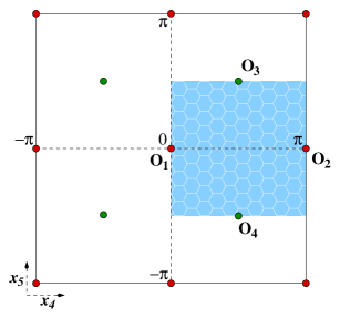
FIG. 1.: Fixed points of the $Z_{2}\times Z^{\prime}_{2}$ orbifolding of the torus, here represented by the whole squared in the $x_{4}$-$x_{5}$ plane. For simplicity, the coordinates are given in units of $R$. The shadowed region corresponds to the actual fundamental space.

It is worth noticing that the distribution of the fixed points is such that the $T^{2}/Z_{2}\times Z^{\prime}_{2}$ orbifolding breaks the translational invariance on the torus down to a discrete translational group, $\cal P$, which maps the equivalent fixed points among themselves. The orbifold also keeps a discrete $Z_{4}$ rotational symmetry around any fixed point. Notice also that, as it is shown in figure 2, the discrete translation ${\cal P^{\prime}}:\vec{y}\rightarrow y^{\prime}$ maps the fundamental space into itself up to the interchange on the $Z_{2}$ and $Z^{\prime}_{2}$ fixed points: $O_{1}\leftrightarrow O_{3}$ and $O_{2}\leftrightarrow O_{4}$, which is equivalent to the exchange of projections: $Z_{2}\leftrightarrow Z^{\prime}_{2}$.

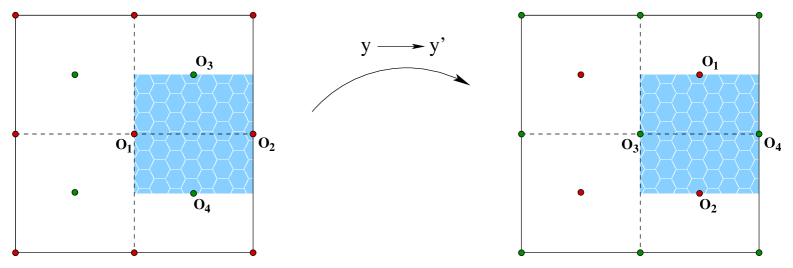
FIG. 2.: Mapping of the orbifold under the discrete translation ${\cal P^{\prime}}:\vec{y}\rightarrow\vec{y}~{}^{\prime}$. Notice that this transformation is equivalent to a redefinition on the projections: $Z_{2}\leftrightarrow Z^{\prime}_{2}$, which interchanges the corresponding fixed points.

The orbifold does not break completely the six dimensional Poincare invariance down to the 4D Poincare group, but it rather keeps an additional discrete subgroup: $Z_{4}\times{\cal P}$, so maintaining the $Z_{8}$ symmetry already existing in the $T^{2}/Z_{2}$ orbifold [5]. This is a remarkable result whose phenomenological consequences we have already mention in section II : (i) the conservation of the extra momentum and (ii) the conservation of the $U(1)_{45}$ symmetry modulus operators with $\Delta\Sigma_{45}=8$; which forbids Majorana neutrinos and introduces a large suppression for proton decay.

B Mode expansion

Any generic field $\varphi(x^{\mu},\vec{y})$ with given $Z_{2}\times Z^{\prime}_{2}$ quantum numbers ($z,z^{\prime}$), for $z,z^{\prime}=\pm$, can be Fourier expanded as

$$\varphi^{(z,z^{\prime})}(x^{\mu},y)=\sum_{n_{1},n_{2}=0}^{\infty}\xi^{(z,z^{\prime})}_{n_{1}n_{2}}(\vec{y})~{}\varphi_{n_{1}n_{2}}(x^{\mu})+\sum_{n_{1},n_{2}=1}^{\infty}\zeta^{(z,z^{\prime})}_{n_{1}n_{2}}(\vec{y})~{}\tilde{\varphi}_{n_{1}n_{2}}(x^{\mu})~{}.$$ (18)

The $\xi^{(z,z^{\prime})}_{n_{1}n_{2}}$ and $\zeta^{(z,z^{\prime})}_{n_{1}n_{2}}$ modes, properly normalized on the fundamental space, are given by

$$\xi^{(+,\pm)}_{n_{1}n_{2}}={\eta_{\vec{n}}\over\pi R}\cos{\vec{n}\cdot\vec{y}\over R}~{};\quad\zeta^{(+,\pm)}_{n_{1}n_{2}}={\sqrt{2}\over\pi R}\cos{\vec{n}\cdot\sigma_{3}\vec{y}\over R}~{};$$ (19)

$$\xi^{(-,\pm)}_{n_{1}n_{2}}={\sqrt{2}\over\pi R}\sin{\vec{n}\cdot\vec{y}\over R}~{};\quad\zeta^{(-,\pm)}_{n_{1}n_{2}}={\sqrt{2}\over\pi R}\sin{\vec{n}\cdot\sigma_{3}\vec{y}\over R}~{};$$ (20)

where both $n_{1}$ and $n_{2}$ are either even or odd numbers for the $(\pm,\pm)$ charged modes, whereas $n_{1}$ should be even (odd) when $n_{2}$ is odd (even) for $(\pm,\mp)$; otherwise the modes are identically zero. Clearly, $\vec{n}$ stands for the vector $(n_{1},n_{2})$. The normalization factor $\eta_{\vec{n}}$ that appears in Eq. (19) is equal to 1 for $\vec{n}=0$ and $\sqrt{2}$ otherwise. Notice that only fields with $(+,+)$ quantum numbers have zero modes.

Using the expansion in Eq. (18), it is easy now to check that the Lagrangian satisfies: ${\cal L}[\varphi^{(z,z^{\prime})}(x^{\mu},\vec{y}~{}^{\prime})]={\cal L}[\varphi^{(z^{\prime},z)}(x^{\mu},\vec{y})]$. That confirms our previous observation that the discrete translation $\vec{y}\rightarrow\vec{y}~{}^{\prime}$ is equivalent to a permutation on the $Z_{2}$ and $Z^{\prime}_{2}$ charges. That also shows the invariance of the lagrangian under the $Z_{4}$ spatial symmetry proper of the $T^{2}/Z_{2}$ orbifold.

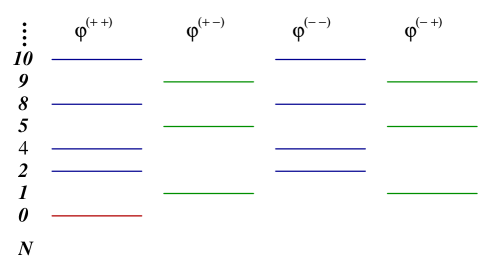
FIG. 3.: KK mass spectrum of a generic field, $\varphi$. The KK index $N=m_{KK}^{2}R^{2}$. Notice that only the (++) fields develop zero modes, and that part of the spectrum has been projected out.

In the effective 4D theory the mass of each mode has the form

$$m_{N}^{2}=m_{0}^{2}+{N\over R^{2}}~{};$$ (21)

with $N=\vec{n}^{2}=n_{1}^{2}+n_{2}^{2}$. In this equation $m_{0}$ is the Higgs vacuum mass contribution, and the physical mass of the zero mode. A typical spectrum of Kaluza Klein (KK) levels is shown in Fig. 3. Except for the zero mode, the spectrum is degenerated and rather complex. Degeneracy for a given mass level depends on the array of $\{n_{1},n_{2}\}$ numbers that give the numerical value $N$. For arrays of the form $\{n,0\}$ (up to a permutation) and $\{n,n\}$, the natural degeneracy of the level is equal to 2. For all other cases the degeneracy is equal to 4. There often are, however, some levels with a larger accidental degeneracy due to some numerical coincidences: some natural numbers have more than one decomposition of the form $N=n_{1}^{2}+n_{2}^{2}$. For instance, one can write $25=5^{2}+0=4^{2}+3^{2}$. Thus, the 6-fold degeneracy of the $N=25$ level sums over the degeneracy of both the decompositions. Table 1. gives the degeneracy of the first KK mass levels for the four classes of $Z_{2}\times Z^{\prime}_{2}$ charges. Notice that the spectrum is only a fourth of the one associated to $T^{2}$. Indeed, the ‘missing’ states have been projected out by the orbifolding. It is worth noticing that the $(\pm,\pm)$ eigenmodes lack the very first (N=1) excited mode, whereas it is present for the $(\pm,\mp)$. Therefore the lightest KK particle on the model will come from these last class of fields.

$N$	$(\pm,\pm)$	$(\pm,\mp)$	$N$	$(\pm,\pm)$	$(\pm,\mp)$
1	—	2	13	—	4
2	2	—	16	2	—
4	2	—	17	—	4
5	—	4	18	2	—
8	2	—	20	4	—
9	—	2	25	—	6
10	4	—	26	4	—

TABLE II.: Level degeneracy according to the $Z_{2}\times Z^{\prime}_{2}$ field charges. Here $N$ labels the physical mass level. A dash indicates a mode that has been projected out from the spectrum by orbifolding. The non degenerated zero mode ($N=0$) has been omitted in this table.

VI $Z_{2}\times Z^{\prime}_{2}$ charge assignments.

A Gauge boson charges: Orbifold symmetry breaking

We now proceed to show the way the gauge and matter fields of our left right model transform under the $Z_{2}\times Z^{\prime}_{2}$ symmetries. We will closely follow a similar prescription to the one given in Reference [7, 18] for the case of five dimensions. We take Gluons and $B-L$ gauge boson to transform under the $Z_{2}$ and $Z^{\prime}_{2}$ projections as follows:

$$G_{\mu}(x,\vec{y})\rightarrow G_{\mu}(x,\vec{y})~{}; G_{a}(x,\vec{y})\rightarrow-G_{a}(x,\vec{y})~{};$$ (22)

$$B_{\mu}(x,\vec{y})\rightarrow B_{\mu}(x,\vec{y})~{}; B_{a}(x,\vec{y})\rightarrow-B_{a}(x,\vec{y})~{};$$ (23)

for $a=4,5$. For the $SU(2)$’s gauge bosons we define the matrix $W=\vec{W}\cdot\vec{\sigma}$. The $Z_{2}\times Z^{\prime}_{2}$ transformation properties of $W_{1,2}$ are then written as

$$W_{\mu}(x^{\mu},\vec{y}) \rightarrow W_{\mu}(x^{\mu},-\vec{y})~{}~{}=~{}\quad PW_{\mu}(x^{\mu},\vec{y})P^{-1}~{};$$ (24)

$$W_{a}(x^{\mu},\vec{y}) \rightarrow W_{a}(x^{\mu},-\vec{y})~{}~{}=~{}-PW_{a}(x^{\mu},\vec{y})P^{-1}~{};$$ (25)

$$W_{\mu}(x^{\mu},\vec{y}~{}^{\prime}) \rightarrow W_{\mu}(x^{\mu},-\vec{y}~{}^{\prime})~{}=~{}\quad P^{\prime}W_{\mu}(x^{\mu},\vec{y}~{}^{\prime})P^{{}^{\prime}-1}~{};$$ (26)

$$W_{a}(x^{\mu},\vec{y}^{\prime}) \rightarrow W_{a}(x^{\mu},-\vec{y}~{}^{\prime})~{}=~{}-P^{\prime}W_{a}(x^{\mu},\vec{y}~{}^{\prime})P^{{}^{\prime}-1}~{};$$ (27)

where $P$, and $P^{\prime}$ are two by two diagonal matrices, acting on the group space, that we chose to be (i) $P~{}=~{}P^{\prime}~{}=~{}diag(1,1)$ for the $SU(2)_{1}$ gauge bosons; and (ii) $P~{}=~{}diag(1,1)$ and $P^{\prime}~{}=~{}diag(1,-1)$, for those of $SU(2)_{2}$.

Above transformation properties can be briefly summarized in terms of the following $Z_{2}\times Z^{\prime}_{2}$ charge assignments:

$$G_{\mu}(+,+);\quad B_{\mu}(+,+);\quad W_{1,\mu}^{3,\pm}(+,+);\quad W^{3}_{2,\mu}(+,+);\quad W^{\pm}_{2,\mu}(+,-);$$ (28)

$$G_{a}(-,-);\quad B_{a}(-,-);\quad W_{1,a}^{3,\pm}(-,-);\quad W^{3}_{2,a}(-,-);\quad W^{\pm}_{2,a}(-,+).$$ (29)

With these assignments, one finds that at the $Z^{\prime}_{2}$ fixed points, $O_{1,2}$, the charged $W^{\pm}_{2,\mu}$ bosons vanish. Thus, the $SU(2)_{2}$ symmetry breaks down to its $U(1)_{I_{3,2}}$ subgroup, whereas all other group factors remain unbroken at such points. In contrast, at the $Z_{2}$ fixed points all the gauge symmetry remains intact. Nevertheless, due to the breaking of the symmetry at two of the fixed points, in the effective four dimensional theory the symmetry is also broken. The residual group is identified as the one on our previous model: $SU(3)_{c}\times SU(2)_{L}\times U(1)_{I_{3R}}\times U(1)_{B-L}$. Notice that this group can also be written as: $[SU(3)_{c}\times SU(2)_{L}\times U(1)_{Y}]\times U(1)_{Y^{\prime}}$. That is the SM symmetry times an extra $U(1)_{Y^{\prime}}$ factor, which is generated by the operator: ${1\over 2}Y^{\prime}\equiv\sqrt{\frac{2}{5}}I_{3,2}-\frac{3}{\sqrt{10}}{1\over 2}(B-L)$. One can easily check this statement by looking at the effective 4D theory. One finds that only the gauge bosons associated with this generator have zero modes, which are massless at this stage.

B Fermion charges

We now turn to the fermion content. In general under the $Z_{2}$ and $Z^{\prime}_{2}$ projections a fermion transforms as

$$\Psi(x^{\mu},\vec{y}) \rightarrow \Psi(x^{\mu},-\vec{y})~{}=~{}\epsilon~{}\Sigma_{45}P\Psi(x^{\mu},y);$$ (30)

$$\Psi(x^{\mu},\vec{y}~{}^{\prime}) \rightarrow \Psi(x^{\mu},-\vec{y}~{}^{\prime})~{}=~{}\epsilon^{\prime}~{}\Sigma_{45}P^{\prime}\Psi(x^{\mu},\vec{y}~{}^{\prime})~{};$$ (31)

where $\epsilon,\epsilon^{\prime}=\pm 1$ are the overall $Z_{2}$ and $Z^{\prime}_{2}$ charges of the six dimensional fermion, respectively. In last equation $P$ and $P^{\prime}$ are the very same matrices used in Eq. (27) which act on the $SU(2)_{1,2}$ group indices. They commute with the $\Sigma_{45}$ matrix that acts on the spinorial space. Clearly, the actual $Z_{2}\times Z^{\prime}_{2}$ charges of each fermionic component depend on the final combination of $\epsilon$’s, $P$’s and the $\Sigma_{45}$ charges. Notice that in the chiral representation, as it is given in the appendix, the $\Sigma_{45}$ operator is diagonal and has the form $\Sigma_{45}=diag(\gamma_{5},-\gamma_{5})$, which indicates that the 4D left and right handed components of a chiral 6D fermion actually hold opposite parities under the $Z_{2}$ and $Z^{\prime}_{2}$ projections. In fact, using the same chiral representation of the appendix, Eq. (31) can be explicitly decomposed in terms of left and right handed components, to get the simplified transformation rules $\Psi_{\pm,R}\rightarrow\pm\epsilon P\Psi_{\pm,R}$ and $\Psi_{\pm,L}\rightarrow\mp\epsilon P\Psi_{\pm,L}$ for $Z_{2}$, and a similar expression for $Z^{\prime}_{2}$.

We take the following ($\epsilon,\epsilon^{\prime}$) assignments for the matter content of the model: ${\cal Q}_{1}(+,+)$; ${\cal Q}^{\prime}_{1}(+,-)$; ${\cal\psi}_{1}(+,+)$; ${\cal\psi}^{\prime}_{1}(-,+)$; ${\cal Q}_{2}(+,+)$; ${\cal Q}^{\prime}_{2}(+,-)$; ${\cal\psi}_{2}(+,-)$; and ${\cal\psi}^{\prime}_{2}(-,-)$. Combining this choice with the one made for the $P$ and $P^{\prime}$ matrices in Eq. (27), it is easy to see that the various fermion representations get the following $Z_{2}\times Z^{\prime}_{2}$ charges, for quarks:

$$Q_{1,L}\equiv\left(\begin{array}[]{c}u_{1L}(+,+)\\ d_{1L}(+,+)\end{array}\right); Q^{\prime}_{1,L}\equiv\left(\begin{array}[]{c}u^{\prime}_{1L}(+,-)\\ d^{\prime}_{1L}(+,-)\end{array}\right);$$ (36)

$$Q_{1,R}\equiv\left(\begin{array}[]{c}u_{1R}(-,-)\\ d_{1R}(-,-)\end{array}\right); Q^{\prime}_{1,R}\equiv\left(\begin{array}[]{c}u^{\prime}_{1R}(-,+)\\ d^{\prime}_{1R}(-,+)\end{array}\right);$$ (41)

$$Q_{2,L}\equiv\left(\begin{array}[]{c}u_{2L}(-,-)\\ d_{2L}(-,+)\end{array}\right); Q^{\prime}_{2,L}\equiv\left(\begin{array}[]{c}u^{\prime}_{2L}(-,+)\\ d^{\prime}_{2L}(-,-)\end{array}\right);$$ (46)

$$Q_{2,R}\equiv\left(\begin{array}[]{c}u_{2R}(+,+)\\ d_{2R}(+,-)\end{array}\right); Q^{\prime}_{2,R}\equiv\left(\begin{array}[]{c}u^{\prime}_{2R}(+,-)\\ d^{\prime}_{2R}(+,+)\end{array}\right);$$ (51)

and for leptons:

$$\psi_{1,L}\equiv\left(\begin{array}[]{c}\nu_{1L}(+,+)\\ e_{1L}(+,+)\end{array}\right); \psi^{\prime}_{1,L}\equiv\left(\begin{array}[]{c}\nu^{\prime}_{1L}(-,+)\\ e^{\prime}_{1L}(-,+)\end{array}\right);$$ (56)

$$\psi_{1,R}\equiv\left(\begin{array}[]{c}\nu_{1R}(-,-)\\ e_{1R}(-,-)\end{array}\right); \psi^{\prime}_{1,R}\equiv\left(\begin{array}[]{c}\nu^{\prime}_{1R}(+,-)\\ e^{\prime}_{1R}(+,-)\end{array}\right);\qquad$$ (61)

$$\psi_{2,L}\equiv\left(\begin{array}[]{c}\nu_{2L}(-,+)\\ e_{2L}(-,-)\end{array}\right); \psi^{\prime}_{2,L}\equiv\left(\begin{array}[]{c}\nu^{\prime}_{2L}(+,+)\\ e^{\prime}_{2L}(+,-)\end{array}\right);$$ (66)

$$\psi_{2,R}\equiv\left(\begin{array}[]{c}\nu_{2R}(+,-)\\ e_{2R}(+,+)\end{array}\right); \psi^{\prime}_{2,R}\equiv\left(\begin{array}[]{c}\nu^{\prime}_{2R}(-,-)\\ e^{\prime}_{2R}(-,+)\end{array}\right).$$ (71)

The zero mode fermion content of the model is the same as the standard model plus an additional sterile neutrino per family. Note that the zero mode spectrum is actually the one of the model discussed in section II. From now one can identify the fermion fields having zero modes with the self-explaining standard notation: $Q,L,u_{R},d_{R},e_{R}$ and $\nu_{s}$.

C Scalar content: Spontaneous symmetry breaking.

The effective 4D gauge symmetry $SU(2)_{L}\times U(1)_{Y}\times U(1)_{Y^{\prime}}$ of the model is being spontaneously broken by an appropriate set of Higgs fields. The minimal set required for this purpose as well to give masses to the SM fermions was introduced in Ref. [7]. It has a bidoublet $\phi(2,2,0)$ and doublets $\chi_{L}(2,1,-1)$ and $\chi_{R}(1,2,-1)$ with the following $Z_{2}\times Z^{\prime}_{2}$ quantum numbers:

$$\phi\equiv\left(\begin{array}[]{cc}\phi^{0}_{u}(+,+)&\phi^{+}_{d}(+,-)\\ \phi^{-}_{u}(+,+)&\phi^{0}_{d}(+,-)\end{array}\right);\quad\chi_{L}\equiv\left(\begin{array}[]{c}\chi^{0}_{L}(-,+)\\ \chi^{-}_{L}(-,+)\end{array}\right);\quad\chi_{R}\equiv\left(\begin{array}[]{c}\chi^{0}_{R}(+,+)\\ \chi^{-}_{R}(+,-)\end{array}\right).$$ (72)

At the zero mode level, only the SM doublet $(\phi^{0}_{u},\phi^{-}_{u})$ and a singlet $\chi^{0}_{R}$ appear. The vacuum expectation values (vev’s) of these fields, namely $\langle\phi^{0}_{u}\rangle=v_{wk}$ and $\langle\chi^{0}_{R}\rangle=v_{R}$, break the SM symmetry and the extra $U(1)_{Y}^{\prime}$ gauge group, respectively. As a matter of fact, in the six dimensional theory, $\langle\chi^{0}_{R}\rangle$ breaks the group $SU(2)_{2}\times U(1)_{B-L}$ down to $U(1)_{Y}$, given a universal mass contribution to all KK $W_{R}$ modes.

VII Mass spectrum and phenomenology.

The analysis of the masses spectrum follows almost identically the one already presented in Ref. [7], with the KK masses now given accordingly to Eq. (21). Vacuum contribution to the masses of all particles is independent of the KK number and directly calculable in the six dimensional theory. Therefore, it introduces a global shifting of the KK spectrum by fixing the value of $m_{0}$, in Eq. (21), for every each field. Mixings in the theory are only produced trough the vacuum, and they are also six dimensional. Thus, no mixing among fields with different KK number is possible. Briefly, these are our main results:

There is no mixing among charged gauge bosons ($W^{\pm}_{L,R}$). The $W_{L}$ zero mode mass is, as usual, $m_{0,W_{L}}^{2}=M_{W_{L}}^{2}=g_{L}^{2}v_{wk}^{2}/2$ whereas, $W_{R}$ gets $m_{0,W_{R}}^{2}={g_{R}^{2}\over 2}\left(v_{R}^{2}+v_{wk}^{2}\right)$. Here, $g_{L,R}$ represent the gauge coupling constants of $SU(2)_{L,R}$ respectively. Notice, that due to its $Z_{2}\times Z^{\prime}_{2}$ charges, $W_{R}$ has no zero mode, and thus, its lower mode gets a $1/R^{2}$ KK mass contribution. Without mixings in this sector, added to KK conservation, most of the former 4D constraints on $v_{R}$ disappear. For instance: there are no new tree level contributions to muon decay. Moreover, $W_{R}$ has not tree level contribution to double beta decay, nor a relevant contribution on the $K-\bar{K}$ mixing (last comes out very suppressed).

On the neutral sector photon decouples and remain massless. the other two neutral gauge bosons mix among themselves. For $v_{R}\gg v_{wk}$, the mass of the standard $Z$ boson gets a mass correction due to this mixing: $M_{Z}^{2}=m_{Z}^{2}-\delta m_{Z}^{2}$, which in the symmetric limit ($g_{L}=g_{R}$) has the form

$${\delta m_{Z}^{2}\over m_{Z}^{2}}\approx{\cos^{2}2\theta\over\cos^{4}\theta}\left({v_{wk}\over v_{R}}\right)^{2}~{},$$ (73)

whereas the mixing is given as

$$\tan\beta\approx\left({v_{wk}\over v_{R}}\right)^{2}{(\cos 2\theta)^{3/2}\over\cos^{4}\theta}~{}.$$ (74)

In these equations $\theta$ corresponds to the standard weak mixing angle. Existence of a mixing in the neutral currents imposes a lower limit on $v_{R}$ that can be calculated as in four dimensions due to the KK conservation. On gets $v_{R}\mathrel{\lower 4.0pt\vbox{\hbox{$>$}\hbox{$\sim$}}}800$ GeV. Limits on $R$ are very weak. Production of KK pair excitations of the $W_{L}$ in colliders [6] imposes a limit that ranges from 400 to 800 GeV. The first KK level for all these neutral fields get a KK mass contribution equal to $2/R^{2}$. They lack the very first possible level of the tower.

The most general Yukawa couplings in the model are

$$h_{u}\bar{Q}_{1}\phi Q_{2}+h_{d}\bar{Q}_{1}\tilde{\phi}Q^{\prime}_{2}+h_{e}\bar{\psi}_{1}\tilde{\phi}\psi_{2}+h^{\prime}_{u}\bar{Q}^{\prime}_{1}\phi Q^{\prime}_{2}+h^{\prime}_{d}\bar{Q}^{\prime}_{1}\tilde{\phi}Q_{2}+h^{\prime}_{e}\bar{\psi}^{\prime}_{1}\tilde{\phi}\psi^{\prime}_{2}+h.c.;$$ (75)

where $\tilde{\phi}\equiv\tau_{2}\phi^{*}\tau_{2}$ is the charge conjugate field of $\phi$. A six dimensional realization of the left-right symmetry, which interchanges the subscripts: $1\leftrightarrow 2$, is obtained provided the $3\times 3$ Yukawa coupling matrices satisfy the constraints: $h_{u}~{}=~{}h^{\dagger}_{u}$; $h^{\prime}_{u}~{}=~{}h^{{}^{\prime}\dagger}_{u}$; $h_{e}~{}=~{}h^{\dagger}_{e};$ $h^{\prime}_{e}~{}=~{}h^{{}^{\prime}\dagger}_{e};$ $h_{d}~{}=~{}h^{{}^{\prime}\dagger}_{d}$. At the zero mode level one obtains the SM Yukawa couplings

$${\cal L}~{}=~{}h_{u}\bar{Q}\phi_{u}u_{R}+h_{d}\bar{Q}\tilde{\phi}_{u}d_{R}+h_{e}\bar{L}\tilde{\phi}_{u}e_{R}+h.c.$$ (76)

It is important to notice that in the above equation $h_{u,e}$ are hermitian matrices, while $h_{d}$ is not. Therefore, whereas $h_{u,e}$ are diagonalizable by a single unitary matrix, $h^{diag}_{u,e}=V_{u,e}h_{u,e}V^{\dagger}_{u,e}$; $h_{d}$ needs two of such matrices: $h^{diag}_{d}~{}=~{}V_{d}h_{d}U^{\dagger}_{d}$. Last implies that, unlike the case of standard left-right models, the left and right handed quark mixings are different from each other. Indeed, for left handed quarks one gets the CKM matrix $U_{CKM}~{}=~{}V^{\dagger}_{u}V_{d}$; while the corresponding right handed charged current mixing matrix for quarks is $U^{R}~{}=~{}V^{\dagger}_{u}U_{d}$.

Considering the decomposition $\bar{\Psi}_{1}\Psi_{2}=\bar{\Psi}_{1,L}\Psi_{2,R}+\bar{\Psi}_{1,R}\Psi_{2,L}$, one can easily read the fermion masses induced by vacuum. Particularly, we find that left and right handed chiral partners (in same representation) have the same mass out of the Yukawa couplings. Also, we stress that all but the neutrino fields, $\nu_{1}$; $\nu^{\prime}_{1}$, $\nu_{2}$; and $\nu^{\prime}_{2}$, get a mass contribution proportional to $v_{wk}$. Standard and sterile neutrinos remain massless at this point. They will get small masses, however, through non renormalizable operators as we will discuss next. It is worth noticing that being neutrinos the particles with the smaller vacuum mass correction, the lightest KK fermionic particle in the model will be a KK neutrino: the ones associated to $\nu^{\prime}_{1}$ and $\nu_{2}$, which have the lowest possible KK mass level with a mass $1/R$.

VIII Neutrino masses

As already mentioned in section V, the orbifolding leaves a residual discrete $Z_{8}$ Lorentz symmetry acting on spinors, which is generated by $\Sigma_{45}$. The conservation of such a symmetry constrains the possible bilinear couplings among fermions. Particularly, as already mentioned, the symmetry forbids a Majorana self coupling for chiral fields. A simple way of understanding this is by noticing that the charge conjugation does not change the 6D chirality (see the appendix), thus, $\bar{\Psi}^{c}_{\pm}~{}\Psi_{\pm}$ has $\Delta\Sigma_{45}=2$. This is troublesome for understanding the smallness of the neutrino mass since without a large Majorana mass, the see-saw mechanism is not any more at work. The problem was already noticed for the six dimensional SM, and an alternative solution was explored in Ref. [19]. Such a solution, however, makes use of singlet bulk neutrinos propagating in a larger (7D) space where the additional dimension is warped [20]. This was similar in spirit to the model of Ref. [21].

As we already remarked in the last section, in our model a Dirac neutrino mass does not come at the renormalizable level of the theory. The model, however, contains neutrinos in both the chiral sectors, and thus a mass term can be written in the effective theory through non renormalizable operators. Such an operator, of course, should be $Z_{8}$ invariant, so it ought to have $\Delta\Sigma_{45}=0$. Looking at the zero mode spectrum of the model we find that all the SM fields ($Q,L,u_{R},d_{R},e_{R}$) have $\Sigma_{45}$ charge equal to $1$, whereas $\nu_{s}$ has $\Sigma_{45}=-1$. Therefore the only possible neutrino mass term at the zero mode level is of the form $\nu^{T}_{sL}C^{-1}\nu_{L}$. As in the previous example, this implies that the neutrino is a Dirac particle. The lowest order operator that contains such a term is of mass dimension eleven:

$${h\over M_{*}^{5}}\bar{\psi}_{1}\tilde{\phi}{~{}\psi^{\prime}_{2}}^{c}\chi_{R}\chi_{R}~{},$$ (77)

which is equivalent to the operator considered in Eq. (2). It generates at the 4D effective theory the suppressed dimension six operator [23]

$\displaystyle{h\over(M_{*}\pi R)^{3}}{{\bar{L}\phi_{u}\nu_{s}^{c}}\chi_{R}^{2}\over M_{*}^{2}}~{}.$which, for $v_{R}\approx 1/\pi R\approx 1$ TeV; $M_{*}\approx 100$ TeV, and a coupling strength of order 0.1 gives $m_{\nu}\sim 1$ eV.

It is remarkable that the model does not need the introduction of singlet bulk neutrinos. Nevertheless, at least one warped or several flat extra dimensions (not seen by the model fields) may be used (though not mandatory) to compensate for the gap between the compactification $R$ and fundamental scale, $M_{*}$. The value of $M_{*}$ we are considering is consistent with current bounds on graviton effects (see for instance Refs. [24]).

IX Baryon non conservation

Turning to the question of proton decay, the considerations are very similar to the $SU(2)_{L}\times U(1)_{I_{3R}}\times U(1)_{B-L}$ model discussed in section II. The residual discrete $Z_{8}$ spatial symmetry of the orbifold naturally constrains the proton life time. All allowed baryon number violating now have to be invariant under the full left-right group and are suppressed down to levels consistent with the experiment as in the $SU(2)_{L}\times U(1)_{I_{3R}}\times U(1)_{B-L}$ model of section II.

The lowest dimension $\Delta B=1$ operators, invariant under gauge and orbifold symmetries in this case are: (i) dimension 16 operators:

$$a) (\bar{\psi}_{1}Q_{2})(\bar{Q}_{1}^{c}\psi^{\prime}_{2})(\bar{Q}_{2}^{c}\not{{D}\hskip 2.15277pt}\psi^{\prime}_{2})~{};$$ (78)

$$b) (\bar{\psi}_{1}\not{{D}\hskip 2.15277pt}Q_{1})(\bar{Q}_{2}^{c}\Gamma^{M}\psi^{\prime}_{2})(\bar{Q}_{2}^{c}\Gamma_{M}\psi^{\prime}_{2})~{};$$ (79)

$$c) (\bar{\psi}_{2}\not{{D}\hskip 2.15277pt}Q_{2})(\bar{Q}_{2}^{c}\Gamma^{M}\psi^{\prime}_{2})(\bar{Q}_{2}^{c}\Gamma_{M}\psi^{\prime}_{2})~{};$$ (80)

where we have considered operators with the smallest number of $\Gamma$’s. The insertion of any product of $\Sigma_{MN}$ matrices will not introduce any new operator to the effective 4D theory. Permutation of $\not{{D}\hskip 2.15277pt}$ and $\Gamma_{M}$ is also allowed. The overall mass suppression on these couplings is of order $M^{-10}$. Thus, at the 4D effective theory one gets the six fermion couplings:

$$a) (\bar{L}d_{R})(\bar{Q}^{c}\nu_{s})(\bar{d}_{R}^{c}\not{{D}\hskip 2.15277pt}\nu_{s})~{};$$ (81)

$$b) (\bar{L}\not{{D}\hskip 2.15277pt}Q)(\bar{d}_{R}^{c}\gamma^{\mu}\nu_{s})(\bar{d}_{R}^{c}\gamma_{\mu}\nu_{s})~{};$$ (82)

$$c) (\bar{e}_{R}\not{{D}\hskip 2.15277pt}d_{R})(\bar{d}_{R}^{c}\gamma^{\mu}\nu_{s})(\bar{d}_{R}^{c}\gamma_{\mu}\nu_{s})~{};$$ (83)

respectively, with and overall suppression $\sim[M_{*}^{6}(M\pi R)^{4}]^{-1}$. The decay modes and predictions for nucleon lifetimes are same as in section II and we do not repeat the discussion here.

X Two component Kaluza-Klein dark matter

In this section, we look at possible dark matter candidates in our model. The fact that in universal extra dimension models with a low compactification scale, KK excitations of photon is stable and can act as a dark matter candidate has been discussed recently[25]. This is however dependent on the nature of the orbifold compactification and in models with $S^{1}/Z_{2}$ orbifold, $\gamma^{1}_{KK}$ is clearly the only possibility. The main reason for this is that, of all the particles at the first KK level, the one with the slowest annihilation rate is the first KK excitation of the photon. First KK excitations of particles such as neutrino or electron which have antiparticles, can annihilate via the exchange of zero mode states (n=0 states) (such as the usual Z-boson) whereas the annihilation of the KK modes of photon can proceed only via the exchange of another KK excitation due to conservation of “fifth” momentum. The latter annihilation cross section is therefore highly suppressed compared to the annihilation rate other particles in the theory. This in turn implies that the $\gamma^{1}_{KK}$ will be present in the late universe in greater abundance than all other KK modes and can play the role of dark matter of the Universe.

When the compactification orbifold is different such as $T^{2}/(Z_{2}\times Z^{\prime}_{2})$ as it is in the left-right symmetric case of this paper, the situation changes drastically. In this case there are two classes of levels: one class corresponding to even KK number with $Z_{2}\times Z^{\prime}_{2}$ quantum numbers $(+,+)$ and $(-,-)$ and another class corresponding to odd KK number, corresponding to $Z_{2}\times Z^{\prime}_{2}$ quantum numbers $(+,-)$ and $(-,+)$. Of these only $(+,+)$ modes contain the zero mode (see Fig. 3). This implies that the lightest KK modes are those in $(+,-)$ or $(-,+)$ class. In these theories the mass of the lowest $\gamma_{KK}$ mode is twice the mass of the lowest KK modes of states $(\pm,\mp)$ type. Therefore the discussion of dark matter candidate has to take this into account to see which particle really is the dark matter. What we find is that the role of dark matter is shared by two different particles: $\gamma^{1}_{KK}$ and $\nu^{1}_{2,KK}$ because the annihilation rate of both of these states are mediated by particles with masses of order $R^{-1}$ and are therefore comparable. In the case of $\gamma^{1}_{KK}$, the exchange particles are the lowest KK modes of the standard model particles and in case of $\nu^{1}_{2,KK}$, they are the $Z^{\prime}$ gauge boson. Below we give semi-quantitative arguments to show that their abundances in the present universe are comparable to each other. The dark matter of the universe should therefore have two components.

To get $\Omega_{X}$ where $X$ denotes either of the above particles, we need their present number density $n_{0}(X)$ and mass. To calculate $n_{0}(X)$, note that if the X-particle decouples from the Hubble expansion at a temperature $T^{*}$, after decoupling, the ratio $n(X,T^{*})/n(\gamma,T^{*})$ does not change except for a predictable fraction which correspond to contributions from particle annihilation to photon density. If we call that fraction $\beta$, the present number density of $n_{0}(X)$ can be written as:

$$n_{0}(X)\simeq\frac{n(X,T^{*})}{n(\gamma,T^{*})}\beta n_{0}(\gamma)$$ (84)

For a given particle $X$, we can roughly estimate $\frac{n(X,T^{*})}{n(\gamma,T^{*})}$ as follows:

$$\frac{n(X,T^{*})}{n(\gamma,T^{*})}~{}=~{}\frac{1.2\sqrt{g^{*}}}{<\sigma_{X}v>}\frac{(T^{*})^{2}}{M_{P\ell}}$$ (85)

where $\sigma_{X}$ denotes the annihilation rate for the pairs of $X$ particles. Thus the relative abundance of the different particles is determined by the magnitude of $\sigma_{X}$, which we estimate below.

For $\gamma^{1}_{KK}$, $\sigma_{X}$ is given by

$$\sigma_{\gamma^{1}_{KK}}\simeq\frac{e^{4}n_{f}}{16\pi M^{2}}$$ (86)

where $M=R^{-1}$ and $n_{f}=\sum_{i}Q^{4}_{i}$, where $Q_{i}$ is the electric charge of the final state particle; $n_{f}\simeq 6$ for our model, where states contributing are all charged leptons (zero modes), quarks and $W^{\pm}$.

On the other hand for $\nu^{1}_{2,L,R}$, the annihilation cross sections are given by:

$$\sigma_{\nu_{2}}\simeq\left(\frac{g_{2}^{2}}{16cos^{2}\theta_{W}M^{2}_{Z^{\prime}}}\right)^{2}2n^{\prime}_{f}$$ (87)

where $g_{2}$ is the weak $SU(2)$-gauge coupling constant. Putting in the values for $g^{2}_{2}\simeq 0.41$ and $sin^{2}\theta_{W}\simeq 0.23$ and taking $M_{Z^{\prime}}$ close to $R^{-1}$, we estimate that $\sigma_{\nu_{2}}\simeq\sigma_{\gamma_{KK}}$. There are two $\nu_{2}$ states (L and R); however, the $\gamma_{KK}$ is twice as massive as the $\nu_{2}$. therefore all three states have nearly same contribution and should equally share the dark matter role. Again one can give a rough evaluation of the contribution of each particle to $\Omega_{X}$ and we find

$$\Omega_{X}\simeq\left(\frac{M}{200~{}GeV}\right)^{2}5~{}KeV$$ (88)

This contribution is roughly of the same order of magnitude as required to give 50% of the critical mass density. Thus we see that the dark matter of the universe in our model has two components to it. This feature should have implications for dark matter detection as well as dark matter annihilation in galaxies. A detailed analysis of these questions will be the subject of a forthcoming investigation.

XI Conclusions

In summary, we have considered local $B-L$ extensions of TeV scale gravity models in six space-time dimensions. We have shown that two problems of TeV scale gravity models having to do with proton decay and neutrino mass can be solved simultaneously with two extra space dimensions compactified on a $T^{2}/Z_{2}$ or $T^{2}/(Z_{2}\times Z^{\prime}_{2})$ orbifold. We have shown how this occurs in two examples: one with the gauge group $SU(2)_{L}\times U(1)_{I_{3R}}\times U(1)_{B-L}$ and another with its left-right symmetric extension. We show that the model can have a compactification scale of order of a TeV and fundamental scale of order 30 to 100 TeV without contradiction with any known phenomenology. The model predicts several interesting decay modes of both the neutron and the proton which under certain circumstances can be within the accessible range of planned proton decay search experiments. We also show that the dark matter of the universe in this picture consists of two components.

A

In a six dimensional space, the $\Gamma^{M}$ Dirac matrices are eight by eight matrices, which can be built from the well known $\gamma^{\mu}$ of the four dimensional representation. Consider the following possible realization:

$$\Gamma^{\mu}=\gamma^{\mu}\otimes\sigma_{1}=\left(\begin{array}[]{cc}0&\gamma^{\mu}\\ \gamma^{\mu}&0\\ \end{array}\right)~{};\qquad\Gamma^{4}=i\gamma_{5}\otimes\sigma_{1}=\left(\begin{array}[]{cc}0&i\gamma_{5}\\ i\gamma_{5}&0\\ \end{array}\right)~{};$$

$$\Gamma^{5}=1_{4\times 4}\otimes i\sigma_{2}=\left(\begin{array}[]{cc}0&1_{4\times 4}\\ -1_{4\times 4}&0\\ \end{array}\right)~{};$$ (A2)

where $\gamma^{5}=-i\gamma^{0}\gamma^{1}\gamma^{2}\gamma^{3}$. It is then easy to see that the above matrices satisfy Clifford algebra: $\{\Gamma^{M},\Gamma^{N}\}=2g^{MN}$ for $M,N=0,1,\dots,5$ and $g^{MN}=diag(1,-1,-1,-1,-1,-1)$, as required.

In this representation one gets

$$\Gamma^{7}=\Gamma^{0}\Gamma^{1}\cdots\Gamma^{5}=\left(\begin{array}[]{cc}1_{4\times 4}&0\\ 0&-1_{4\times 4}\\ \end{array}\right)~{};$$ (A3)

whereas the generator of rotations in the $x_{4}-x_{5}$ plane, that is the $U(1)_{45}$ Lorentz subgroup, is given by

$$\Sigma_{45}={i\over 2}~{}[\Gamma^{4},\Gamma^{5}]~{}=~{}\left(\begin{array}[]{cc}\gamma_{5}&0\\ 0&-\gamma_{5}\\ \end{array}\right)~{}.$$ (A4)

Notice that $[\Sigma_{45},\Gamma^{7}]=0$; thus, one can further classify the fermion components in terms of the $\Sigma_{45}$ eigenstates, that is through out the $U(1)_{45}$ charge.

Furthermore, we take the four dimensional Dirac matrices in its well known chiral representation:

$$\gamma^{\mu}=\left(\begin{array}[]{cc}0&\sigma^{\mu}\\ \bar{\sigma}^{\mu}&0\\ \end{array}\right)~{};$$ (A5)

for $\sigma^{\mu}=(1_{2\times 2},\vec{\sigma})$, with $\vec{\sigma}$ the Pauli matrices, and $\bar{\sigma}^{\mu}=(1_{2\times 2},-\vec{\sigma})$. In this representation $\gamma_{5}$ has a totally diagonal form: $\gamma_{5}=diag(1_{2\times 2},-1_{2\times 2})$.

$\Gamma^{7}$ has two chiral eigenstates defined as $\Psi_{+}$ and $\Psi_{-}$. Clearly, any six dimensional fermion, $\Psi$, is decomposed in the chiral representation in terms of its chiral components as

$\displaystyle\Psi=\left(\begin{array}[]{c}\Psi_{+}\\ \Psi_{-}\end{array}\right)~{}.$Let us stress that six dimensional chirality does not correspond to four dimensional chirality. Six dimensional chiral fields, indeed, correspond to four component fermions, that still contain two 4D chiral components, identified as usual as left (L) and right (R) handed components, eigenstates of $\gamma^{5}$:

$\displaystyle\Psi_{\pm}=\left(\begin{array}[]{c}\psi_{\pm,R}\\ \psi_{\pm,L}\end{array}\right)~{}.$

Charge conjugated fields are defined as usual by the transformation $\Psi^{c}=C\bar{\Psi}^{T}$, where $C$ is such that $(\Gamma^{M})^{T}=-C\Gamma^{M}C^{-1}$. It is easy to check that in the chiral 6D representation $C=\Gamma^{0}\Gamma^{2}\Gamma^{4}$. The operator $C$ also satisfies the identities $C^{\dagger}=C^{-1}=-C$. Notice also that because $\{C,\Sigma_{45}\}=0$, charge conjugation changes the $U(1)_{45}$ charge. Moreover, as $[C,\Gamma^{7}]=0$, thus charge conjugation does not affect the six dimensional chirality. Specifically we have $(\Psi_{\pm})^{c}=(\Psi^{c})_{\pm}$, in contrast to what happens in four dimensions. The straightforward implication of this property is the absence of a Majorana mass term for a single chiral fermion. Indeed, the corresponding Lorentz invariant bilinear that one can write with a single field and its conjugate needs both its chiral components to couple in the form:

$\displaystyle\bar{\Psi}^{c}~{}\Psi=\bar{\Psi}^{c}_{+}~{}\Psi_{-}+\bar{\Psi}_{-}^{c}~{}\Psi_{+}~{}.$Actually this is just as in the case of the Dirac mass couplings, which, as in four dimensions, also need both the chiralities to be written:

$\displaystyle\bar{\Psi}~{}\Psi=\bar{\Psi}_{+}~{}\Psi_{-}+\bar{\Psi}_{-}~{}\Psi_{+}~{}.$

REFERENCES

- [1] I. Antoniadis, Phys. Lett. B 246 (1990) 377; E. Witten, Nucl. Phys. B471, 135 (1996); J. Lykken, Phys. Rev. D 54, 3693 (1996); N. Arkani-Hamed, S. Dimopoulos and G. Dvali, Phys. Lett. B 429, 263 (1998); Phys. Rev. D59, 086004 (1999); I. Antoniadis, N. Arkani-Hamed, S. Dimopoulos and G. Dvali, Nucl. Phys. B 516, 70 (1998); K. Dienes, E. Dudas and T. Gherghetta, Phys. Lett. B 436, 55 (1998).
- [2] M. Gell-Mann, P. Ramond and R. Slansky, in Supergravity, eds. P. van Niewenhuizen and D.Z. Freedman (North Holland 1979); T. Yanagida, in Proceedings of Workshop on Unified Theory and Baryon number in the Universe, eds. O. Sawada and A. Sugamoto (KEK 1979); R.N. Mohapatra and G. Senjanović, Phys. Rev. Lett. 44, 912 (1980).
- [3] K. R. Dienes, E. Dudas and T. Gherghetta, Nucl. Phys. B557, 25 (1999); N. Arkani-Hamed, S. Dimopoulos, G. Dvali and J. March-Russell, hep-ph/9811448.
- [4] G. Dvali and A.Y. Smirnov, Nucl. Phys. B563, 63 (1999); R. N. Mohapatra and A. Pérez-Lorenzana, Nucl. Phys. B 593, 451 (2001); R. N. Mohapatra and A. Pérez-Lorenzana, Nucl. Phys. B 576, 466 (2000); R. Barbieri, P. Creminelli and A. Strumia, Nucl.Phys. B 585, 28 (2000).
- [5] T. Appelquist, B.A. Dobrescu, E. Ponton, Ho-U. Yee, Phys. Rev. Lett. 87, 181802 (2001).
- [6] T. Appelquist, H. C. Cheng and B. Dobrescu, Phys. Rev. D 64, 035002 (2001).
- [7] R. N. Mohapatra and A. Pérez-Lorenzana, Phys. Rev. D66, 035005 (2002).
- [8] B. Dobrescu and E. Poppitz, Phys. Rev. Lett. 87, 031801 (2001).
- [9] M.B. Green, H. Schwarz, Phys. Lett. B 149, 117 (1984).
- [10] C. Berger et al. [Frejus Collaboration], Phys. Lett. B269, 227 (1991).
- [11] S. Seidel et al., Phys. Rev. Lett.61, 2522 (1988).
- [12] Y. Kamyshkov, Proceedings of NNN1 workshop, Stony Brook, ed. C. K. Jung (1999).
- [13] N. Borghini, Y. Gouverneur, M. H.G. Tytgat, Phys. Rev. D 65, 025017 (2002).
- [14] M. Fabrichesi, M. Piai, G. Tasinato, Phys. Rev. D64, 116006 (2001).
- [15] L. Alvarez-Gaumé, E. Witten, Nuc. Phys. B 234, 269 (1984).
- [16] E. Witten, Phys. Lett. B 117, 324 (1982).
- [17] S. Elitzur, V. P. Nair, Nucl. Phys. B243, 205 (1984); E. Kiritsis, Phys. Lett. B 178, 53 (1986); M. Bershadsky and C. Vafa, hep-th/9703167.
- [18] K. Mimura and S. Nandi, hep-ph/0203126.
- [19] T. Appelquist, B.A. Dobrescu, E. Ponton, Ho-U. Yee, hep-ph/0201131.
- [20] L. Randall and R. Sundrum, Phys. Rev. Lett. 83, 3370 (1999).
- [21] Y. Grossman and M. Neubert, Phys. Lett. B474 (2000) 361;
- [22] G. Perez, hep-ph/0208102.
- [23] For a related discussion on the use of higher dimension operators for generating neutrino masses see for instance: K.S. Babu, C.N. Leung, Nucl.Phys. B619, 667 (2001); A. Pérez-Lorenzana and C.A. de S. Pires, Phys. Lett. B 522, 297 (2001).
- [24] C.D. Hoyle, et. al, Phys. Rev. Lett.86, 1418 (2001). G. F. Giudice, R. Rattazzi and J. D. Wells, Nucl. Phys. B 544, 3 (1999); V. Barger, T. Han, C. Kao and R. J. Zhang, Phys. Lett. B 461, 34 (1999); E. A. Mirabelli, M. Perelstein and Michael E. Peskin, Phys. Rev. Lett. 82, 2236 (1999); S. Hannestad, G.G. Raffelt, Phys. Rev. Lett. 88, 071301 (2002).
- [25] G. Servant and T. Tait, hep-ph/0206071; H. C. Cheng, J. Feng and K. Matchev, hep-ph/0207125.