Unbiased analysis of CLEO data at NLO and pion distribution amplitude

Abstract

We discuss different QCD approaches to calculate the form factor $F^{\gamma^{*}\gamma\pi}(Q^{2})$ of the $\gamma^{*}\gamma\to\pi^{0}$ transition giving preference to the light-cone QCD sum rules (LCSR) approach as being the most adequate. In this context we revise the previous analysis of the CLEO experimental data on $F^{\gamma^{*}\gamma\pi}\left(Q^{2}\right)$ by Schmedding and Yakovlev. Special attention is paid to the sensitivity of the results to the (strong radiative) $\alpha_{s}$-corrections and to the value of the twist-four coupling $\delta^{2}$. We present a full analysis of the CLEO data at the NLO level of LCSRs, focusing particular attention to the extraction of the relevant parameters to determine the pion distribution amplitude, i.e., the Gegenbauer coefficients $a_{2},~{}a_{4}$. Our analysis confirms our previous results and also the main findings of Schmedding and Yakovlev: both the asymptotic, as well as the Chernyak–Zhitnitsky pion distribution amplitudes are completely excluded by the CLEO data. A novelty of our approach is to use the CLEO data as a means of determining the value of the QCD vacuum non-locality parameter $\lambda^{2}_{q}=\langle{\bar{q}D^{2}q}\rangle/\langle{\bar{q}q}\rangle=0.4\text{ GeV}^{2}$, which specifies the average virtuality of the vacuum quarks.

I Introduction

Recently, the CLEO collaboration CLEO98 has measured the $\gamma^{*}\gamma\to\pi^{0}$ form factor $F^{\gamma^{*}\gamma\pi}(Q^{2})$ with high precision. This data has been processed by Schmedding and Yakovlev (SY) SchmYa99 using light-cone QCD sum rules (LCSR), taking also into account the perturbative QCD contributions in the next-to-leading order (NLO) approximation. In this way SY obtained useful constraints on the shape of the pion distribution amplitude (DA) in terms of confidence regions for the Gegenbauer coefficients $a_{2}$ and $a_{4}$, the latter being the projection coefficients of the pion DA on the corresponding eigenfunctions. Note that SY have extended to the NLO the LCSR approach suggested before by Khodjamirian Kho99 for the leading order (LO) light-cone sum rule method.

The present analysis gives further support to the claim, expressed by the above mentioned authors, that LCSRs provide the most appropriate basis in describing the form factor of the $\gamma^{*}\gamma\to\pi^{0}$ transition. This is intimately connected with peculiarities of real-photon processes in QCD RR96 ; Kho99 . But the method of the CLEO data processing, adopted in SchmYa99 , seems to be not quite complete from our point of view. We think that an optimal analysis should take into account the correct ERBL evolution of the pion DA to the scale $Q^{2}_{\text{exp}}$ of the process (the latter not to be fixed at some average point, $\mu_{\text{SY}}=2.4$ GeV, as done in SchmYa99 ) and to re-estimate the contribution $\delta^{2}$ from the next twist term. The influence of both these effects appears to be important and it is examined here in detail. Furthermore, we are not satisfied with the error estimation performed in the SY analysis, for reasons to be explained later, and prefer therefore to use a more traditional treatment to determine the sensitivity to the input parameter $\delta^{2}$ and the construction of the 1-$\sigma$ and 2-$\sigma$ error contours.

Our main goal in the present work will be to obtain new constraints on the $(a_{2},~{}a_{4})$ DA parameters from the CLEO data, taking into account all the remarks mentioned above, and then to compare them with the constraints following from QCD SRs with nonlocal condensates (NLC). We will not repeat here the derivation of the main results of LCSRs, as well as those related to NLC SRs, but we will refer the interested reader to Kho99 ; SchmYa99 and correspondingly to BMS01 ; BM02 and references therein. But for the sake of convenience we included a technical exposition of our approach in comprehensive appendices.

The paper is organized as follows. In Sec. II we review different QCD approaches to calculate the transition form factor $F^{\gamma^{*}\gamma\pi}(Q^{2})$, having recourse to QCD “factorization theorems” ERBL79 , encompassing both perturbation theory and LCSRs. The analysis of the CLEO data is discussed in Sec. III in conjunction with the SY approach in comparison with other approaches/approximations. In Sec. IV we present a complete NLO analysis of the CLEO data with a short discussion of the BLM setting procedure. Sec. V includes a comparison of the QCD SR pion DA models with the results obtained in Sec. IV from the CLEO data processing. In Sec. VI we summarize our conclusions. The paper ends with five appendices: in Appendix A we re-estimate the value of the twist-four scale $\delta^{2}$. In Appendix B the old Chernyak–Zhitnitsky (CZ) result for $a_{2}$ is discussed, paying attention to evolution effects. In Appendices C and D the two-loop results DaCh81 ; KMR86 for the purely perturbative part of the form-factor calculations and the ERBL evolution of the pion DA are outlined. Finally, in Appendix E, all needed calculation details for the NLO LCSR are presented.

II Transition form factor $\mathbf{F^{\gamma^{*}\gamma\pi}(Q^{2})}$ with LCSR

II.1 Factorization of the $\mathbf{F^{\gamma^{*}\gamma^{*}\pi}}$ form factor. Standard results

The form factor of the process $\gamma^{*}(q_{1})\gamma^{*}(q_{2})\to\pi^{0}(p)$ is defined by the matrix element

$$\int d^{4}ze^{-iq_{1}z}\langle{\pi^{0}(p)\mid T\{j_{\mu}(z)j_{\nu}(0)\}\mid 0}\rangle=i\epsilon_{\mu\nu\alpha\beta}q_{1}^{\alpha}q_{2}^{\beta}F^{\gamma^{*}\gamma^{*}\pi}(Q^{2},q^{2})\,,$$ (1)

where $q_{1}+q_{2}=p$, $Q^{2}=-q_{1}^{2}>0$ with $q^{2}=-q_{2}^{2}\geq 0$ are the virtualities of the photons, $j_{\mu}=(\frac{2}{3}\bar{u}\gamma_{\mu}u-\frac{1}{3}\bar{d}\gamma_{\mu}d)$ is the quark electromagnetic current, and $\pi^{0}(p)$ is the pion state with momentum $p$. If both virtualities, $Q^{2}$ and $q^{2}$, are sufficiently large, the $T$-product of the currents in (1) can be expanded near the light-cone $z^{2}=0$. This expansion results in factorization theorems, which control the structure of the form factor ERBL79 at leading twist. As a result, the form factor can be cast in the form of a convolution over the momentum fraction variable $x$ (of the total momentum $p$) to read

$$F_{\text{QCD}}^{\gamma^{*}\gamma^{*}\pi}(Q^{2},q^{2})=f_{\pi}\int\limits_{0}^{1}\!\!dx\,\,T(Q^{2},q^{2};\mu_{\text{F}}^{2};x)\varphi_{\pi}(x;\mu_{\text{F}}^{2})\equiv f_{\pi}T(Q^{2},q^{2};\mu_{\text{F}}^{2};x)\mathop{\otimes}\limits_{x}\varphi_{\pi}(x;\mu_{\text{F}}^{2})\,.$$ (2)

The hard amplitude $T(Q^{2},q^{2};x)$ – playing the role of the Wilson coefficient in the OPE – is calculable within QCD perturbation theory (PT):

$$T=T_{0}+\frac{\alpha_{s}(\mu_{\text{R}}^{2})}{4\pi}T_{1}+\left[\frac{\alpha_{s}(\mu_{\text{R}}^{2})}{4\pi}\right]^{2}T_{2}+\ldots\,,$$ (3)

while the pion DA $\varphi_{\pi}(x;\mu_{\text{F}}^{2})$ contains the long-distance effects and demands the application of nonperturbative methods. Due to factorization theorems, DAs enter as the central input of various QCD calculations of hard exclusive processes. The LO term $T_{0}$ in (3) depends only on kinematical variables, but the NLO amplitude $T_{1}$, calculated in DaCh81 ; KMR86 , depends also on the factorization scale $\mu_{\text{F}}^{2}$:

$$T_{0}(Q^{2},q^{2};x) \equiv N_{T}C_{0}(Q^{2},q^{2};x)\ =\ N_{T}\left[\frac{1}{Q^{2}x+q^{2}(1-x)}+(x\to 1-x)\right]\,;$$ (4)

$$T_{1}(Q^{2},q^{2};\mu_{\text{F}}^{2};x) = N_{T}\left[\ln\left(\frac{\bar{Q}^{2}}{\mu_{\text{F}}^{2}}\right)\cdot C_{0}(Q^{2},q^{2};u)\mathop{\otimes}\limits_{u}V_{0}(u,x)+C_{1}(Q^{2},q^{2};x)\right]\,.$$ (5)

Here, $N_{T}\equiv(e_{u}^{2}-e_{d}^{2})/\sqrt{2}=\sqrt{2}/6$ is the QCD normalization factor, $\bar{Q}^{2}=-\left[(q_{1}-q_{2})/2\right]^{2}=(Q^{2}+q^{2})/2$, and $\mu_{\text{R}}^{2}$ and $\mu_{\text{F}}^{2}$ denote, respectively, the scale of renormalization of the theory and the factorization scale of the process. $C_{0,1}$ and $V_{0,1}$ are, respectively, the perturbative expansion elements of the coefficient function $C$ of the process and the ERBL kernel $V$ in the LO (subscript 0) and NLO (subscript 1) approximation . The structure of $T_{1}$ is discussed in more detail in KMR86 ; MuR97 and in Appendix C.1. Here we only recall those features relevant for our discussion: Eq. (5), which specifies the definition of the coefficient function $C_{1}$ is a consequence of the QCD factorization theorems ERBL79 . Due to these theorems, the first logarithmic term in Eq. (5), originating from collinear divergences, can be absorbed into the renormalization of the DA, $\varphi_{\pi}(x;\mu_{\text{F}}^{2})$, following the ERBL equation (see App. D, Eq. (D.1)). Namely, the formal solution of the ERBL equation in the 1-loop approximation is

$$\varphi_{\pi}(x;\mu^{2}_{0})\stackrel{{\scriptstyle\text{ERBL}}}{{\longrightarrow}}\varphi_{\pi}^{\text{RG}}(x;\mu^{2}) = \exp\left[\int_{\alpha_{s}(\mu_{0}^{2})}^{\alpha_{s}(\mu^{2})}da\frac{aV_{0}\ }{\beta(a)}\mathop{\otimes}\limits\right]\varphi_{\pi}(x;\mu_{0}^{2})$$ (6)

(here $\beta(a)=-b_{0}a^{2}$ is the 1-loop $\beta$-function). We adopt here as a factorization scale $\mu_{\text{F}}^{2}=Q^{2}$. For that case, $F^{\gamma^{*}\gamma^{*}\pi}$, obtained in Eq. (2) at the scale $\mu^{2}$, can be transformed into

$$F^{\gamma^{*}\gamma^{*}\pi}\to F^{\gamma^{*}\gamma^{*}\pi}_{\text{RG}}(Q^{2},q^{2})=f_{\pi}\left[T_{0}(Q^{2},q^{2};x)+\frac{\alpha_{s}(\mu_{\text{R}}^{2})}{4\pi}T_{1}(Q^{2},q^{2};Q^{2};x)\right]\mathop{\otimes}\limits_{x}\varphi_{\pi}^{\text{RG}}(x;Q^{2})\,.$$ (7)

To fix the renormalization scale $\mu_{\text{R}}^{2}$, one needs to go beyond the NLO approximation. In the absence of such information and in order to further simplify the NLO analysis, we also set $\mu_{\text{R}}^{2}=\mu_{\text{F}}^{2}=Q^{2}$. It is useful to expand $\varphi_{\pi}^{\text{RG}}(x;\mu^{2})$ over the eigenfunctions $\psi_{n}(x)$ of the one-loop ERBL equation, i.e., in terms of the Gegenbauer polynomials $C^{3/2}_{n}(\xi)$,

$$\varphi_{\pi}^{RG}(x;\mu^{2})=\sum_{n=0,2,4,\ldots}a_{n}(\mu^{2})\cdot\psi_{n}(x)\,;\quad a_{0}=1;~{}\psi_{n}(x)\equiv 6x(1-x)C^{3/2}_{n}(2x-1)\,.$$ (8)

In this representation, all the dependence on $\mu^{2}$ is contained in the coefficients $a_{n}(\mu^{2})$ and is dictated by the ERBL equation. Different reasons, explained in SchmYa99 and BMS01 ; BM02 , point to the possibility of retaining only the first 3 terms in this expansion. Following then this approximation, the form factor can be parameterized by only two variables $a_{2}(\mu_{0}^{2})$ and $a_{4}(\mu_{0}^{2})$ that accumulate the mesonic large-distance effects (at some scale $\mu_{0}^{2}$).

A special case of the OPE appears when one of the photons ($q_{2}$) is near the mass shell. It is instructive to present here an evident NLO perturbative expression for Eq. (7) in the formal limit $q^{2}\to 0$ (cf. Eq. (C.8) in Appendix C),

$$F_{\text{PT}}^{\gamma^{*}\gamma\pi}(Q^{2}) = \frac{\sqrt{2}}{Q^{2}}f_{\pi}\left\{1+\Sigma(Q^{2})+\frac{\alpha_{s}(Q^{2})}{4\pi}C_{\text{F}}\left[-5+7.9\cdot\Sigma(Q^{2})-3.8\cdot\Delta(Q^{2})\right]\right.$$ (9)

$$\qquad\qquad\left.-\frac{80}{27}\frac{\delta^{2}(Q^{2})}{Q^{2}}\right\}$$

with $\Sigma(Q^{2})\equiv a_{2}(Q^{2})+a_{4}(Q^{2})$ and $\Delta(Q^{2})\equiv a_{2}(Q^{2})-a_{4}(Q^{2}).$

On the r.h.s. of Eq. (9), the twist-four contribution is included in terms of the twist-four asymptotic DAs, presented in Kho99 . The coefficients $a_{2,4}(Q^{2})$ and the twist-four coupling $\delta^{2}(Q^{2})$ are evolved to the scale $Q^{2}$ using, correspondingly, the renormalization group (RG) equation to NLO and LO accuracy.

II.2 Why do we need LCSRs for the transition form factor?

A straightforward calculation of $F^{\gamma^{*}\gamma\pi}(Q^{2})$ in QCD is not possible. In particular, at the formal limit $q^{2}\to 0$, it is not sufficient to retain only a few terms of the light-cone OPE of (1). One has, in addition, to take into account the interaction of the small-virtuality photon at large distances proportional to $O(1/\sqrt{q^{2}})$, (for a recent discussion, consider section 4 in RR96 and MuR97 ). The LCSR method allows one to avoid the problem of the photon long-distance interaction by providing the means of performing all QCD calculations at sufficiently large $q^{2}$ and then use a dispersion relation to return to the mass-shell photon. To isolate the dangerous neighborhood of $q^{2}=0$, one should apply an appropriate realistic model for the spectral density at low $s$, based, for instance, on quark-hadron duality. Using this sort of analysis and by employing analyticity and duality arguments, the following expression was obtained in Kho99

$$F_{\text{LCSR}}^{\gamma^{*}\gamma\pi}(Q^{2})=\int\limits_{0}^{s_{0}}\!\!\frac{ds}{m_{\rho}^{2}}\,\mathbf{Im}\left[\frac{1}{\pi}\,F_{\text{QCD}}^{\gamma^{*}\gamma^{*}\pi}(Q^{2},s)\right]\,e^{\left(m_{\rho}^{2}-s\right)/M^{2}}+\int\limits_{s_{0}}^{\infty}\!\!\frac{ds}{s}\,\mathbf{Im}\left[\frac{1}{\pi}\,F_{\text{QCD}}^{\gamma^{*}\gamma^{*}\pi}(Q^{2},s)\right]\,.$$ (10)

$F_{\text{QCD}}^{\gamma^{*}\gamma^{*}\pi}(Q^{2},s)$ on the r.h.s. of (10) is taken from Eq. (2) and the Borel parameter is $M^{2}\approx 0.7$ GeV², whereas $m_{\rho}$ is the $\rho$-meson mass and $s_{0}=1.5$ GeV² denotes the effective threshold in the $\rho$-meson channel.

This program has first been suggested in general form in Kho99 and was realized there for the LO approximation of the process. Taking $F_{\text{QCD}}^{\gamma^{*}\gamma^{*}\pi}$ at LO in $\alpha_{s}$, the form factor $F_{\text{LOLC}}^{\gamma^{*}\gamma\pi}(Q^{2})$ was obtained from Eq. (10) with

$$F_{\text{LO QCD}}^{\gamma^{*}\gamma^{*}\pi}(Q^{2},q^{2})=f_{\pi}N_{T}\left\{C_{0}(Q^{2},q^{2};u)\mathop{\otimes}\limits_{u}\varphi_{\pi}(u)-\frac{1}{2}\left[C_{0}(Q^{2},q^{2};u)\right]^{2}\mathop{\otimes}\limits_{u}\varphi^{(4)}_{\pi}(u)\right\}\,$$ (11)

and

$$\mathbf{Im}\left[\frac{1}{\pi}\,F_{\text{LO QCD}}^{\gamma^{*}\gamma^{*}\pi}(Q^{2},s)\right]=\frac{f_{\pi}\sqrt{2}}{3}\left[\frac{\varphi_{\pi}(u)}{s+Q^{2}}-\frac{1}{Q^{2}}\frac{d\varphi^{(4)}(u)}{ds}\right]_{u=Q^{2}/(s+Q^{2})}\,.$$ (12)

Here, the numerically important twist-four contribution was also included using a simple asymptotic expression for the twist-four DA contribution Kho99

$$\varphi^{(4)}(u,\mu^{2})=\frac{80}{3}\delta^{2}(\mu^{2})u^{2}(1-u)^{2}\,.$$ (13)

Note that the coupling $\delta^{2}$ is determined from the matrix element

$$\langle{\pi(p)|g_{s}\bar{d}\tilde{G}_{\alpha\mu}\gamma^{\alpha}u|0}\rangle=i\delta^{2}f_{\pi}p_{\mu}\,.$$ (14)

The estimates for $\delta^{2}(\mu^{2})$, including also its RG-evolution, are presented in Appendix A.

II.3 The framework of NLO LCSR for the form factor

An application of the above scheme to the NLO was more recently performed in SchmYa99 . The $\alpha_{s}$-corrections to this process are expected to be rather large, of the order of 20% (see, e.g., MuR97 ). The size of these corrections can be roughly estimated from the perturbative expressions for their asymptotic parts by comparing to each other the values $1$ and $\displaystyle-5\frac{\alpha_{s}}{4\pi}C_{\text{F}}$ in Eq. (9). Therefore, for a quantitative description of the form factor, this contribution should be taken into account. This important step was done by Schmedding and Yakovlev, who have used the NLO perturbative expression for $F_{\text{QCD}}^{\gamma^{*}\gamma^{*}\pi}$ in Eq. (10),

$$F_{\text{NLO QCD}}^{\gamma^{*}\gamma^{*}\pi}(Q^{2},q^{2};\mu^{2})=F_{\text{LO QCD}}^{\gamma^{*}\gamma^{*}\pi}(Q^{2},q^{2})+\frac{\alpha_{s}(\mu^{2})}{4\pi}f_{\pi}T_{1}(Q^{2},q^{2};\mu^{2};x)\mathop{\otimes}\limits_{x}\varphi_{\pi}(x;\mu^{2})\,,$$ (15)

where $\mu^{2}\equiv\mu_{\text{F}}^{2}=\mu_{\text{R}}^{2}\neq Q^{2}$, to construct a NLO version of the LCSR for the form factor $F^{\gamma^{*}\gamma\pi}(Q^{2})$. The spectral density $\mathbf{Im}[F_{\text{NLO QCD}}^{\gamma^{*}\gamma^{*}\pi}(Q^{2},s;\mu^{2})]/\pi$, based on Eq. (15), depends on the scale $\mu^{2}$. In the original paper SchmYa99 , this scale was fixed by relating it to the mean value of $Q^{2}$ with respect to the CLEO experimental data, i.e., by setting $\mu^{2}=\mu_{\text{SY}}^{2}=$ $\langle{Q_{\text{exp}}^{2}}\rangle\approx(2.4)^{2}~{}{\text{GeV}^{2}}$. Use of Eq. (15) implies that one accounts for the scale dependence in $\varphi_{\pi}(x;Q^{2})$ (e.g., for the different CLEO points) via the leading order perturbative formula

$$\varphi_{\pi}(x;Q^{2})\approx\left[1+\frac{\alpha_{s}(\mu^{2})}{4\pi}\ln\left(Q^{2}/\mu^{2}\right)\cdot V_{0}(x,u)\right]\mathop{\otimes}\limits_{u}\varphi_{\pi}(u;\mu^{2})\,,$$

rather, than using the RG expression, given by Eq. (6). This seems to be a rather crude approximation, given that other reference points are evolved with $\mu^{2}$ by utilizing the NLO ERBL evolution equation.

III CLEO data analysis revisited

Let us scrutinize the form factor approaches, discussed above, in close comparison with the CLEO data CLEO98 .

III.1 Theoretical approaches to the CLEO data

In this subsection – in order to be in close analogy with the original SY paper – we shall adopt their scale definition of the CZ DA. It is worth noting, however, that the genuine CZ DA differs from that definition because it is determined at the much lower normalization scale $\mu_{0}=0.5$ GeV (a discussion of this important point is relegated to Appendix B). To distinguish the two models in the present analysis, we will use in what follows a special notation: (i) CZ DA parameters originating from the SY prescription ($a_{2}^{\text{CZ}}(\mu^{2}=0.5~{}{\text{GeV}^{2}})=2/3$), and by using a 2-loop evolution to the scale $\mu^{2}_{\text{SY}}$, will be denoted with the superscripts CZSY, whereas (ii) those conforming with our prescription ($a_{2}^{\text{CZ}}(\mu^{2}=1~{}{\text{GeV}^{2}})=0.56$, see Appendix B) and being 2-loop evolved to the scale $\mu^{2}_{\text{SY}}$ will be marked by the superscripts CZ.

        

Figure 1: The plane ($a_{2},a_{4}$) and results of different analyses of the CLEO data for the form factor $F_{\pi\gamma\gamma}(Q^{2})$. We show here the best-fit points of LO LCSR, NLO LC SR (SY) and a NLO PT analysis for two values of the twist-four coupling $\delta^{2}=0.2~{}{\text{GeV}^{2}}$ (a) and $\delta^{2}=0.18~{}{\text{GeV}^{2}}$ (b). The solid contours correspond to a $1\sigma$-criterion, while the broken ones to a $2\sigma$-criterion. We also plot for comparison the positions of the CZSY (◼) and the asymptotic (◆) DAs. All values are evaluated at $\mu^{2}=(2.4~{}{\text{GeV}})^{2}$. The inclined straight line on the right hand-side of the figure is the modified diagonal $a_{2}+a_{4}/3=$const, corresponding to the new $1\sigma$-ellipse of the NLO LCSR analysis.

The status of these approximations (NLO PT, LO LCSR and NLO LCSR) is illustrated in Fig. 1 by the relative positions of the corresponding admissible regions for these parameters in the $(a_{2},a_{4})$ plane. Here, the regions enclosed by the needle-like- and ellipse-like solid contours correspond to a $1\sigma$-deviation criterion (CL=68%) PDG2000 , while the broken contours refer to a $2\sigma$-deviation criterion (CL=95%). Note that these contours have been derived by taking into account only the statistical error bars in CLEO98 (see their Table 1). This marks a crucial difference between our processing of the data and that in SchmYa99 , where the “theoretical-systematic uncertainties” have been involved in the statistical analysis together with the statistical ones. In other words, we do not “smear” the quantities $\delta^{2}$ (or $a_{0}=1$) over their corresponding (theoretical) error-bar intervals. In our opinion, such a manner would require an additional substantiation and further suggestions about the distribution of these errors that we want to avoid in our analysis. Hence, instead of that, we process the data at a few fixed values of $\delta^{2}$ in order to clarify the sensitivity of the results to this parameter.

It should be clear that a really admissible region might be somewhat larger than the presented “purely statistical” contours in Fig. 1, a price one has to pay for our strict way of data processing.

1. The large contour, enclosing the origin, corresponds to the LO LCSR form factor, discussed in Kho99 . Note that the point denoting the position of the asymptotic DA lies just on the periphery of the $1\sigma$-contour and that the CZ DA one (see Kho99 ), lies far outside.

2. The needle-like contour on the left top corner of both parts of Fig. 1 corresponds to Eq. (9) and is stretched along the “diagonal” $a_{2}+0.75\cdot a_{4}=$ const. The weak dependence of Eq. (9) on $\Delta\equiv a_{2}-a_{4}$ slightly turns the angle of the diagonal $\simeq 3\pi/4\to 0.8\pi$. On the other hand, taking into account the evolution with $Q^{2}$ of $a_{2}$ and $a_{4}$ for every $Q^{2}_{\text{exp}}$ makes the contour finite – much like a “diagonal” needle-like strip. As we have mentioned above, the formal limit of the NLO expression, Eq. (9), cannot give a reliable result for the form factor. In this context it is interesting to mention that the corresponding contour is located outside the regions determined by the LCSRs. Furthermore, all known DA models (see, e.g., Table 1) and the phenomenological predictions (BKM00 ; BMS01 and references therein) are located far away from this contour – clearly demonstrating the poor reliability of the corresponding perturbative approach.

3. At least the heavy-line contours (enclosing also the SY point SchmYa99 ) correspond to the SY approximation. These contours do not overlap with those corresponding to the LO LCSR ones – even at the $2\sigma$-deviation level. Therefore, $\alpha_{s}$-corrections are crucially important in extracting the DA parameters. Our best-fit point with respect to the NLO LCSR is close to but not coinciding with the one presented by SY (compare entries 3 and 4 in Table 1). In Fig. 1(a) the full circle inside the contour is just the SY point. The best-fit points, corresponding to different approximations and models, considered in the present analysis, are collected in Table 1, where the notation $\chi^{2}_{\text{(d.o.f.)}}=\chi^{2}/14$ has been used (in correspondence to the number 15 of the CLEO experimental data points).

Table 1: Compilation of best-fit points shown in Fig. 1(a) with $\delta^{2}(1~{}{\text{GeV}^{2}})=0.20$ GeV².

Best-fit points/models	$a_{2}(\mu_{\text{SY}}^{2})$	$a_{4}(\mu_{\text{SY}}^{2})$	$\chi^{2}_{\text{(d.o.f.)}}$
NLO PT (9) best fit	$-0.44$	$+0.40$	$0.49$
LO LCSR best fit	$+0.04$	$-0.19$	$0.48$
NLO LCSR best fit	$+0.20$	$-0.17$	$0.48$
SY LCSR SchmYa99	$+0.19$	$-0.14$	$0.49$
BMS model BMS01	$+0.13$	$-0.08$	$0.74$
CZSY DA SchmYa99	$+0.28$	$-0.009$	$1.8$
CZ DA CZ84	$+0.35$	$-0.006$	$3.6$
Asympt. DA	$-0.006$	$+0.00$	$3.0$

It should be stressed that the admissible region (heavy-line contours), obtained with our data-processing procedure, differs from that in SchmYa99 . Our contours look slightly larger than theirs despite the fact that possible theoretical/systematic uncertainties were not included in our consideration. Just because of this latter reason, our contours possess another orientation relative to those of SY, as one appreciates by comparing Fig. 1(a) and Fig. 2 with Fig. 6 in SchmYa99 . Moreover, the CZSY DA model appears to be seemingly closer ($\chi^{2}=1.8$) to the best-fit point $(0.20,-0.17)$ than the asymptotic one ($\chi^{2}\approx 3$). But the genuine CZ DA with $a_{2}^{\text{CZ}}(\mu_{\text{SY}}^{2})=0.35$ and $a_{4}^{\text{CZ}}(\mu_{\text{SY}}^{2})=-0.006$ (consult the discussion in Appendix B) generates a value of $\chi^{2}=3.6$, which is larger than that of the asymptotic DA.

The best-fitted linear combination of $a_{2},~{}a_{4}$, that determines the large axis of the NLO LCSR contour (see Fig. 1(a)) and parameterizes its orientation, is found to be

$$a_{2}+\frac{1}{3}\cdot a_{4}=0.143,$$ (16)

instead of $a_{2}+0.6\cdot a_{4}=0.11\pm 0.03$, reported in SchmYa99 . Note that the SY point also belongs to the diagonal: $a_{2}^{\text{SY}}+1/3\cdot a_{4}^{\text{SY}}\approx 0.143$. The coefficient $1/3$ in (16) can be predicted without any fitting; it is solely determined by the structure of the NLO LCSR (10). Indeed, Eq. (10) can be rewritten as SchmYa99

$$A_{0}(Q^{2},\mu^{2}_{\text{SY}})+A_{2}(Q^{2},\mu^{2}_{\text{SY}})\cdot a_{2}(\mu^{2}_{\text{SY}})+A_{4}(Q^{2},\mu^{2}_{\text{SY}})\cdot a_{4}(\mu^{2}_{\text{SY}})=Q^{2}\cdot F^{\gamma^{*}\gamma\pi}(Q^{2})$$

(to be compared with the fit given in Eq. (16)) and the discussed coefficient expresses the average value of the ratio $A_{4}(Q^{2},\mu^{2}_{\text{SY}})/A_{2}(Q^{2},\mu^{2}_{\text{SY}})$. Notice that this ratio, averaged over the CLEO data range $\{Q^{2}_{\text{exp}}\}$, amounts to 0.31, while the r.h.s. of Eq. (16) is determined by the experimental data on the form factor. The coefficient $0.6$, obtained in the SY fit SchmYa99 , can be associated with the same ratio at the mean value $\mu_{\text{SY}}^{2}=\langle{Q^{2}_{\text{exp}}}\rangle$. The ratio $A_{4}(Q^{2})/A_{2}(Q^{2})$ is a concave function in $Q^{2}$ and, therefore, its mean value, $\langle{A_{4}(Q^{2})/A_{2}(Q^{2})}\rangle$, is smaller than its value, $A_{4}(\mu_{\text{SY}}^{2})/A_{2}(\mu_{\text{SY}}^{2})$, at the “mean point” $\mu_{\text{SY}}^{2}$.

III.2 Sensitivity to input parameters

As it turns out, the location of the admissible $a_{2},~{}a_{4}$ regions is rather sensitive to the value of the input parameter $\delta^{2}$. To illustrate this point, we have repeated the data processing with an admissible (near its low boundary) value $\delta^{2}=0.18~{}{\text{GeV}^{2}}$ (see Appendix A). All contours in Fig. 1(b) shift closer to the asymptotic point (◆), but their relative positions do not drastically change and, hence, the main conclusions (i-iii) of the previous subsection remain valid. The results of this data processing are presented in Fig. 1(b) and in Table 2. One appreciates that the hierarchy of the different models (lower parts of both Tables) with respect to the NLO LCSR best fit does not change, though the values of $\chi^{2}$ can change significantly. Indeed, the point marking the BMS model moves from the $2\sigma$-deviation level at $\delta^{2}=0.2~{}{\text{GeV}^{2}}$ (see Table 1) inside the $1\sigma$-deviation region near the SY LCSR point at $\delta^{2}=0.18~{}{\text{GeV}^{2}}$ (cf. row 5 in Table 2). Therefore, the value of $\delta^{2}$ and, in general, also the value of the twist-four term can substantially affect the locations of the admissible regions. But all other options, like the CZ DA and the asymptotic DA, remain excluded at the $2\sigma$–deviation level.

Table 2: Compilation of best fit points shown in Fig. 1(b) with $\delta^{2}(1~{}{\text{GeV}^{2}})=0.18$ GeV².

Best-fit points/models	$a_{2}(\mu_{\text{SY}}^{2})$	$a_{4}(\mu_{\text{SY}}^{2})$	$\chi^{2}_{\text{(d.o.f.)}}$
NLO PT (9) best fit	$-0.37$	$+0.34$	$0.49$
LO LCSR best fit	$+0.006$	$-0.14$	$0.49$
NLO LCSR best fit	$+0.17$	$-0.14$	$0.48$
SY LCSR SchmYa99	$+0.19$	$-0.14$	$0.51$
BMS model BMS01	$+0.13$	$-0.08$	$0.56$
CZSY DA SchmYa99	$0.28$	$-0.009$	$2.2$
CZ DA CZ84	$+0.35$	$-0.006$	$4.2$
Asympt. DA	$-0.006$	$+0.00$	$2.3$

Let us pause for a moment and turn our attention to a recent paper by Diehl et al. DKV01 . The authors of this work employ a purely perturbative QCD approach to analyze the CLEO data without taking into account the twist-four contribution, i.e., using Eq. (9) with $\delta^{2}(Q^{2})=0$. They consider this treatment justified given the possible large uncertainties in estimating the twist-four contribution (which in the SY procedure is taken to be $\pm 20$%). Comparing their results with those of Schmedding and Yakovlev SchmYa99 , Diehl et al. correctly note that the relative weights of $a_{2}(\mu_{0}^{2})$ and $a_{4}(\mu_{0}^{2})$ in $F^{\gamma^{*}\gamma\pi}$ display a much stronger $Q^{2}$-dependence than in the leading-twist case with the consequence that the allowed SY parameter region becomes much smaller than in their approach. However, the size of the twist-four contribution is crucial for accurately extracting the parameters $a_{2}$ and $a_{4}$ – as we have just demonstrated. Therefore in our analysis we use a different approach: the value of $\delta^{2}$ is connected with the parameter $\lambda_{q}^{2}$ of the vacuum non-locality. We first fix the value of $\lambda_{q}^{2}$ and then we allow for the parameter $\delta^{2}$ to vary in a 10% range. The whole uncertainty in $\delta^{2}$ for the selected range of $\lambda_{q}^{2}=0.4-0.6$ GeV² amounts then to about 30% in accordance with Kho01 . This strategy enables us to use the CLEO data as a direct measure (a vacuum detector) to select that model for the QCD vacuum, which provides the best agreement between theory and experiment.

IV Complete two-loop analysis of the CLEO data

In the previous section we have demonstrated the high sensitivity of the DA parameters $(a_{2},~{}a_{4})$ to strong radiative corrections for the form factor, as well as to the scale of the twist-four contribution (see Fig. 1 a(b) and BMS01 ). Therefore, to obtain these parameters from the CLEO data in a reliable way, one should take into account the radiative corrections in the most accurate possible way. To this end, we want to improve in this section the accuracy of the extraction procedure of $(a_{2},~{}a_{4})$ at the NLO level. A new estimate for $\delta^{2}$, the magnitude of the twist-four contribution, is also introduced in the present analysis (see below). We also briefly discuss an attempt to go beyond the level of the NLO, having recourse to a recent calculation MNP01a of the radiative correction based on the BLM scale setting.

IV.1 Complete NLO analysis

Here we use the complete 2-loop expression for the form factor $F^{\gamma^{*}\gamma^{*}\pi}(Q^{2},q^{2})$, given by Eq. (7). For this reason, we put $\mu^{2}=Q^{2}$ in (15) so that for the quantities

$$\alpha_{s}(\mu^{2})\stackrel{{\scriptstyle\rm RG}}{{\longrightarrow}}\alpha_{s}(Q^{2}),~{}~{}\varphi_{\pi}(x;\mu^{2})\stackrel{{\scriptstyle\rm ERBL}}{{\longrightarrow}}\varphi_{\pi}(x;Q^{2})=U(\mu^{2}\to Q^{2})\varphi_{\pi}(x;\mu^{2}),\,$$

the NLO evolution is implied. Then, we substitute the spectral density $\rho(Q^{2},s;\mu^{2}=Q^{2})$, derived in SchmYa99 (see the text below Eq. (15)), in LCSR (10) to obtain $F^{\gamma^{*}\gamma\pi}(Q^{2})$ in a regular manner and to fit the CLEO data over $Q^{2}\in\{Q^{2}_{\text{exp}}\}$. The evolution $\varphi_{\pi}(x;Q^{2})=U(\mu^{2}_{\text{SY}}\to Q^{2})\varphi_{\pi}(x;\mu^{2}_{\text{SY}})$ is performed for every point $Q^{2}_{\text{exp}}$, with the aim to return to the normalization scale $\mu^{2}_{\text{SY}}$ and to extract the DA parameters $(a_{2},~{}a_{4})$ at this reference scale. Stated differently, for every measurement, $\{Q_{\text{exp}}^{2},F^{\gamma^{*}\gamma\pi}(Q_{\text{exp}}^{2})\}$, its own factorization/renormalization scheme has been used so that the NLO radiative corrections are taken into account in a complete way.

The accuracy of the procedure is, nevertheless, still limited owing to the mixing of the NLO and the LO approximations. Indeed, the value of the twist-four coupling $\delta^{2}(\mu^{2})$, as well as its RG-evolution with $\mu^{2}$, are estimated in the LO approximation. This quantity enters the LCSR formula (15) together with the NLO-part and can lead to an additional uncertainty. In order to improve the theoretical accuracy of the values of $a_{2}$ and $a_{4}$, extracted from the CLEO data, one has to re-estimate the twist-four contribution, $\delta^{2}(1~{}{\text{GeV}^{2}})$, with a better accuracy.

To summarize, our data processing procedure differs from the SY one in the following points:

1. $\alpha_{s}(\mu^{2})$ is the exact solution of the 2-loop RG equation, rather than the approximate (but popular in the HEP community) expression (C.15) PDG2000 , that was used in the SY analysis.

2. All logarithms $\ln(Q^{2}/\mu^{2})$ are absorbed into the evolution of the pion DA, performed separately at each experimental point $Q_{\text{exp}}$ (compare Eqs. (6), (7) with Eq. (15)). The corresponding expressions for the form factor are collected in Appendix E.

3. The value of the parameter $\delta^{2}$ has been re-estimated to read $\delta^{2}(1{\text{GeV}^{2}})=0.19\pm 0.02~{}{\text{GeV}^{2}}$ (see Appendix A), and this value has been used in the data processing.

This processing of the CLEO data produces the admissible regions, one of which, corresponding to $\delta^{2}=0.19~{}{\text{GeV}^{2}}$, is shown in Fig. 2(a), where the original SY regions (Fig. 6 in SchmYa99 ) are also presented in Fig. 2(d) for the ease of comparison.

     

     

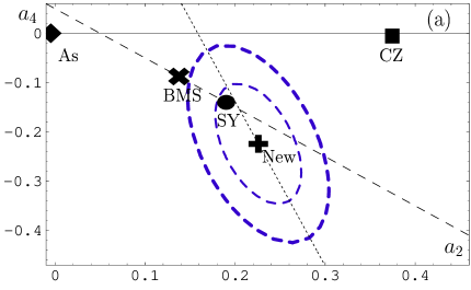
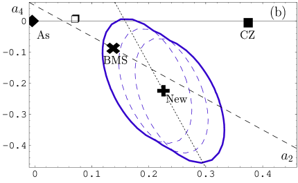
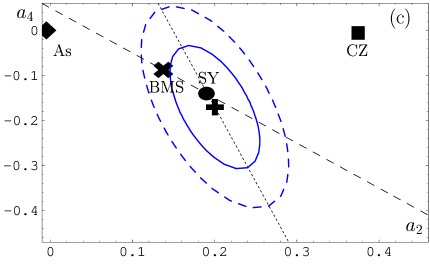
Figure 2: Results of the analysis of the CLEO data for the form factor $F_{\pi\gamma^{*}\gamma}(Q^{2})$ in terms of fiducial areas in the plane ($a_{2}$,$a_{4}$). (a) We show the best fit point of the new NLO LC SRs (✚, termed “New”, which is associated with the value of the twist-four coupling $\delta^{2}=0.19~{}{\text{GeV}^{2}}$, and display by the heavy (broken) contour the regions corresponding to a $1\sigma$ ($2\sigma$)-deviation. We also show the SY point (⚫), the BMS point (✖), the asymptotic point (◆), and the CZ point (◼) - all evolved to the SY scale. The inclined straight dotted line in the left figure is the modified diagonal $a_{2}+0.3a_{4}=0.159$, whereas the inclined straight dashed line is the original diagonal $a_{2}+a_{4}=$const. (b) We show three $2\sigma$-regions (dashed contours), obtained for different values of the twist-four parameter: $\delta^{2}=0.17,\ 019,\ 0.21~{}{\text{GeV}^{2}}$ and also their unification: $2\sigma$-contour (thick line). All points and straight lines are as in Fig. 2(a), except ❒, which denotes a brand-new result obtained on a transverse lattice Dal02 . (c) The contours of the previous NLO analysis à la SY and the “old” best-fit point (✚) are presented for comparison (cf. the lower right corner of Fig. 1(a) and use the scale of Fig. 2(a)). (d) The original SY plot (note the different scales on the axes and the symbol ◼ denoting the CZSY DA) is shown for comparison. All values shown are evaluated at the scale $\mu=2.4$ GeV.

To produce the complete $2\sigma$- and $1\sigma$-contours, corresponding to $\delta^{2}(1{\text{GeV}^{2}})=0.19\pm 0.02~{}{\text{GeV}^{2}}$, we need to unite three regions obtained for different values of the twist-four parameter: $\delta^{2}=0.17,\ 019,\ 0.21~{}{\text{GeV}^{2}}$. This procedure is illustrated in Fig. 2(b) using as an example the $2\sigma$-contour. Let us remind the reader in this context that the SY contours are stretched along the “LO perturbative” diagonal $a_{2}+a_{4}=$const (the dashed straight line on the l.h.s. resembles exactly this diagonal) while the solid (dotted) contours correspond to the 1 $\sigma$ (2 $\sigma$) regions. This stretching of the contours appears here because of the SY manner of the data processing, namely, because the theoretical uncertainties of the input parameters were also involved in the statistical analysis.

Table 3: Compilation of best-fit points shown in Fig. 2(a) with $\delta^{2}(1~{}{\text{GeV}^{2}})=0.19$ GeV².

Best-fit point/models	$a_{2}(\mu_{\text{SY}}^{2})$	$a_{4}(\mu_{\text{SY}}^{2})$	$\chi^{2}_{\text{(d.o.f.)}}$	$a_{2}+0.3\cdot a_{4}$
New NLO LCSR best fit	$+0.23$	$-0.22$	$0.47$	$0.159$
SY NLO LCSR SchmYa99	$+0.19$	$-0.14$	$0.59$	$0.153$
BMS model BMS01	$+0.14$	$-0.09$	$1.0$	$0.113$
Asymptotic model	$-0.002$	$+0.00$	$4.3$	$-0.00$
CZ model CZ84	$+0.43$	$-0.003$	$4.3$	$0.43$

The new best-fit point (✚, “New”), as well as the whole $\sigma$-contours themselves appear to be displaced in Fig. 2(a) (approximately) along the new diagonal (cf. Eq. (16)),

$$\quad a_{2}+0.3\cdot a_{4}=0.16\pm 0.007\,.$$ (17)

In Fig. 2(c) we present for comparison the contours of the previous NLO analysis in the sense of SY (low right corner of Fig. 1(a)) drawn, however, at the scale of Fig. 2(a). The positions of the best-fit points and models are provided in Table 3.

It should be clear from our discussion that these new contours are somewhat smaller than the previous ones (Fig. 2(c)), but slightly larger than the original SY ones (Fig. 2(d)), and show another orientation along the diagonal Eq. (17). The difference between the new regions, determined in the present analysis, and those of the SY one is remarkable. For instance, the SY point appears now near the boundary and inside the $1\sigma$-region in Fig. 2(a). Moreover, the preliminary (i.e., for $a_{4}=0$) SY best-fit point, $a^{\prime}_{2}=0.12\pm 0.03$ SchmYa99 , and the phenomenological estimates for ($a_{2},~{}a_{4}$), presented in BKM00 , ($a_{4}=0,~{}a_{2}~{}(1~{}{\text{GeV}^{2}})=0.1\pm 0.1$), lie on the boundary of the united $2\sigma$-region (see Fig. 2(b)).

IV.2 Beyond the NLO approximation: effects from BLM scale-setting

The renormalization scale $\mu_{\text{R}}^{2}$ in Eq. (7) can be fixed by a NNLO calculation of $T_{2}$ following the BLM prescription. Recently, the NNLO contribution to $C_{2}$, proportional to $b_{0}$ and required for the BLM scale setting, was obtained in MNP01a for a kinematics with $q_{2}^{2}=0$. As an exercise, let us perform the new fit to obtain the scale $\mu_{\text{R}}^{2}=\mu^{2}_{\text{BLM}}$ and the best-fit point $\{a^{\text{BLM}}_{2},a^{\text{BLM}}_{4}\}$ for the NLO expression given by Eq. (9). We follow the same procedure as in Sec. III.1, replacing this time $\alpha_{s}(Q^{2})\to\alpha_{s}(\mu^{2}_{\text{BLM}}(a_{2},a_{4},Q^{2}))$ in Eq. (9), where for $\mu^{2}_{\text{BLM}}(a_{2},a_{4},Q^{2})$ Eq. (7.7) from MNP01a is used. As it turns out, practically for all points in the considered domain in the lower half-plane $a_{4}\leq 0$, the BLM setting leads to the condition $\mu^{2}_{\text{BLM}}\ll Q^{2}$, in conformance with the results of MNP01a . Therefore, for this region, the BLM setting seems to rule out predictions from the NLO perturbation theory.

Only for points within a rather thin strip in the upper half-plane $a_{4}>0$ (cf. Eqs. (7.2a), (7.7) in MNP01a ), the BLM setting gives $\mu^{2}_{\text{BLM}}>Q^{2}$. Interestingly, the case discussed in Sec. III.1 (ii) and based on Eq. (9) belongs just to this thin strip. The corresponding $(a_{2},a_{4})$ values are displayed below for comparison together with the initial result (second row) without the BLM setting.

$$a^{\text{BLM}}_{2}(\mu_{\text{SY}}^{2})=-0.55, \ \ a^{\text{BLM}}_{4}(\mu_{\text{SY}}^{2})=0.48 \mu^{2}_{R}=\mu^{2}_{\text{BLM}}\approx Q^{2}/0.35$$ (18)

$$a_{2}(\mu_{\text{SY}}^{2})=-0.44, \ \ ~{}~{}~{}~{}~{}a_{4}(\mu_{\text{SY}}^{2})=0.40\ \mu^{2}_{R}=Q^{2}\,.$$

To calculate the imaginary part $\mathbf{Im}F_{\text{QCD}}^{\gamma^{*}\gamma^{*}\pi}(Q^{2},s)$, used in Eq. (10), one needs to know the NNLO contribution proportional to $b_{0}$ for $q_{2}^{2}\neq 0$, which is still not computed. For this reason, the results obtained with the BLM scale setting fall out of the region of the NLO LCSR analysis. The calculation of the complete NNLO contribution or, at least, its convolution with $\varphi_{as}$ is a very demanding task that has not been accomplished yet.

V Pion DA from QCD SR vs CLEO data

Let us now turn to the important topic of whether the CLEO data is consistent with the non-local QCD SR results for $\varphi_{\pi}$. We present in Fig. 3 the results of the data analysis for three central values of the coupling $\delta^{2}(\mu^{2}=1~{}{\text{GeV}^{2}})=0.19,0.235,0.29~{}{\text{GeV}^{2}}$, which in turn correspond to three admissible values of the vacuum non-locality parameter $\lambda_{q}^{2}=0.4,0.5,0.6~{}{\text{GeV}^{2}}$. For each value of $\lambda_{q}^{2}$ from this ensemble, we define the corresponding central value of $\delta^{2}$ and its uncertainty (for details, see Appendix A). Then, we process the CLEO data as described in the previous section and obtain the complete $2\sigma$- and $1\sigma$-contours on the plane $(a_{2},a_{4})$, following from the CLEO experiment. An example of these regions is represented in Fig. 2(b) and is also displayed in Fig. 3(a), where the $2\sigma$-contour is shown as a solid line and the $1\sigma$-contour as a dashed one.

The task now is to compare these new constraints with those following from the QCD SRs with nonlocal condensates. We have established in BMS01 that a two-parameter model $\varphi_{\pi}(x;a_{2},a_{4})$ really enables one to fit all the moment constraints for $\langle\xi^{N}\rangle_{\pi}$ that result from NLC QCD SRs (see MR89 for more details). The only parameter entering the NLC SRs is the correlation scale $\lambda^{2}_{q}$ in the QCD vacuum, known from nonperturbative calculations and lattice simulations (for a discussion and references, see Appendix A).

  

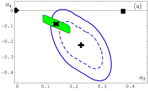
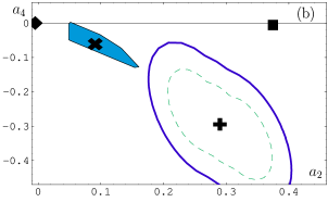
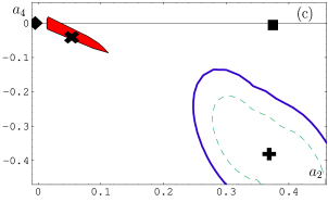
Figure 3: Three $2\sigma$-contours of the admissible regions following from the analysis of the CLEO data for different values of $\delta^{2}$: (a) – for $\lambda^{2}_{q}=0.4~{}{\text{GeV}^{2}}$ and $\delta^{2}=(0.19\pm 0.02)~{}{\text{GeV}^{2}}$; (b) – for $\lambda^{2}_{q}=0.5~{}{\text{GeV}^{2}}$ and $\delta^{2}=(0.235\pm 0.025)~{}{\text{GeV}^{2}}$; (c) – for $\lambda^{2}_{q}=0.6~{}{\text{GeV}^{2}}$ and $\delta^{2}=(0.29\pm 0.03)~{}{\text{GeV}^{2}}$. Solid lines in all figures enclose the $2\sigma$-contours, whereas the $1\sigma$-contours are enclosed by dashed lines. The three slanted and shaded rectangles represent the constraints on ($a_{2},~{}a_{4}$) posed by the QCD SRs BMS01 for corresponding values of $\lambda^{2}_{q}=0.4,~{}0.5,~{}0.6$ GeV² (from left to right). All values are evaluated at $\mu=2.4$ GeV after evolution. The marked points are explained in Fig. 2, except for the point marked with ✖. This point represents here the BMS solution, which corresponds to a particular value of $\lambda_{q}^{2}$.

The three slanted and shaded rectangles in Fig. 3 are the constraints on the Gegenbauer coefficients ($a_{2},~{}a_{4}$) resulting from the NLC QCD SRs at different values of $\lambda^{2}_{q}=0.4,~{}0.5,~{}0.6$ GeV² , BMS01 ; BM02 . The overlap of the displayed regions in Fig. 3 can serve as a means of determining the appropriate value of $\lambda^{2}_{q}$. In fact, one may conclude that the value $\lambda^{2}_{q}=0.4$ GeV² is more preferable relative to the higher values of $\lambda^{2}_{q}$. It should be noted, however, that even for this lowest value of that scale, the agreement with the constraints in Fig. 3 is rather moderate and of similar quality as using the SY constraints BMS01 ; BM02 . It is tempting to test even smaller values of $\lambda^{2}_{q}$ than $0.4$ GeV² in the NLC SR as an attempt to improve the agreement with the CLEO constraints in Fig. 3. But such values appear to be at the lower limits for the $\lambda^{2}_{q}$ estimates from non-perturbative approaches (see Appendix A). Furthermore, the NLC SR becomes unstable at such low values of $\lambda^{2}_{q}$. As a result, the accuracy of the DA moments is rather poor and the final constraint on ($a_{2},~{}a_{4}$) becomes unreliable. Taking into account all these arguments, we think that an improvement of the ingredients of the NLC ansatz may provide a better agreement with the CLEO data than just using $\lambda^{2}_{q}<0.4$ GeV² .

VI Conclusions

In this paper we have studied the theoretical predictions for the pion transition form factor $F^{\gamma^{*}\gamma\pi}(Q^{2})$ in comparison with the CLEO experimental data CLEO98 on this form factor. We have presented a full analysis of this data and contrasted the results with those found in the context of QCD LCSR at the NLO level. In this way, we have revised and improved the procedure of analyzing the CLEO data, first performed by Schmedding and Yakovlev in SchmYa99 . The main goal has been to obtain constraints on the shape of the pion DA of twist-2, $\varphi_{\pi}(x;a_{2},a_{4})$ in the most accurate way. The values of the crucial parameters, viz. the twist-four coupling $\delta^{2}(\mu^{2})$ and $\alpha_{s}(\mu^{2})$, involved in this procedure, have been treated more accurately than in previous approaches. The main findings may be summarized as follows.

1. We have tested different kinds of approximations to calculate $F^{\gamma^{*}\gamma\pi}(Q^{2})$ and revealed how the size of $\alpha_{s}$ and the twist-four corrections can affect the admissible regions of the DA parameters $(a_{2},a_{4})$.

2. New admissible regions for the $(a_{2},a_{4})$ parameters, see Figs. 2(b), 3(a), – different from those in SchmYa99 – have been obtained, though the constraints do not change drastically in the sense that the initial SY best-fit point still belongs to a $1\sigma$-deviation region (CL=68%) in this space, whereas the CZ DA and also the asymptotic one are definitely excluded at the level of a $2\sigma$-deviation criterion (CL=95%). Moreover, one may appreciate by comparing Figs. 2(a, b) with Fig. 2(d) that this exclusion with respect to the asymptotic DA becomes even more pronounced using our data processing.

3. The bunch of admissible pion DAs, $\varphi^{BMS}_{\pi}(x;a_{2},a_{4})$, corresponding to the estimate $\lambda^{2}_{q}=0.4$ GeV², that was constructed within the framework of QCD SRs with nonlocal condensates in BMS01 , compares well (at the $2\sigma$–level) with the new more restrictive constraints obtained in the present investigation as Fig. 3 demonstrates. In addition, half of the calculated admissible region intersects with the $1\sigma$ domain as well, see Fig. 3(a).

Appendix A Revision of the QCD SR results for $\delta^{2}$

The coupling $\delta^{2}(\mu^{2})$ was originally estimated in NSVZ84 and found to be $\delta^{2}(\mu^{2}=1~{}{\text{GeV}^{2}})=0.2\pm 0.02~{}{\text{GeV}^{2}}$. Here, we re-analyze the QCD SR for $\delta^{2}$, derived in OPiv88 , which is based on a non-diagonal correlator of the quark-gluon and quark (pseudoscalar) currents. This SR relates $\delta^{2}$ to $\lambda_{q}^{2}$ and determines the value of the ratio $\displaystyle r=\lambda_{q}^{2}/(2\delta^{2})$. Evaluating the SR leads to the estimate $r>1$ and consequently to $\lambda_{q}^{2}/2>\delta^{2}$. Moreover, $r$ is rather sensitive to the size of the radiative corrections. In this work, we use $\Lambda_{3}^{\text{LO}}=312~{}{\text{MeV}}$, obtained recently in a DIS fit of the CCFR data in KPS02 that leads to $\alpha_{s}^{\text{LO}}(1~{}{\text{GeV}^{2}})\approx 0.59$. The same sort of analysis in the NLO approximation leads to the estimate $\Lambda_{3}^{\text{NLO}}=410~{}{\text{MeV}}$ that is indeed not far from the standard value $380~{}{\text{MeV}}$ (Appendix C.2).

To determine $\delta^{2}$, we first fix the parameter $\lambda_{q}^{2}$ by employing the “conservative estimate” $\lambda_{q}^{2}(\mu^{2}=1~{}{\text{GeV}^{2}})=0.4$ GeV². In QCD the value of this parameter was estimated in the QCD SR approach BI82 and also using lattice data BM02 :

$$\lambda_{q}^{2}=\frac{\langle{\bar{q}(0)\nabla^{2}q(0)}\rangle}{\langle{\bar{q}(0)q(0)}\rangle}\begin{array}[]{c}\text{\footnotesize in chiral}\\ =\\ \text{\footnotesize limit}\end{array}\frac{\langle{\bar{q}(0)\left(ig\,\sigma_{\mu\nu}G^{\mu\nu}\right)q(0)}\rangle}{2\langle{\bar{q}(0)q(0)}\rangle}=\left\{\begin{array}[]{ll}0.4\pm 0.1~{}{\text{GeV}^{2}}&\text{\cite[cite]{\@@bibref{Authors Phrase1YearPhrase2}{BI82,OPiv88}{\@@citephrase{(}}{\@@citephrase{)}}}}\\ 0.4-0.5~{}{\text{GeV}^{2}}&\text{\cite[cite]{\@@bibref{Authors Phrase1YearPhrase2}{BM02}{\@@citephrase{(}}{\@@citephrase{)}}}}\end{array}\right.\ .$$ (A.1)

A brief review of the different estimates of $\lambda_{q}^{2}$ is given in BM02 .

The evaluation of the SR for the quantity $r$,

$$\frac{\lambda_{q}^{2}}{2\delta^{2}}\equiv r(M^{2},\varrho,s_{0})=\frac{\displaystyle 1-\varrho\cdot\exp\left(-m^{2}_{\pi^{\prime}}/M^{2}\right)}{\displaystyle 1+\frac{2\pi^{2}}{9}\frac{\langle{G^{2}}\rangle}{\lambda_{q}^{2}M^{2}}-\frac{2\alpha_{s}(1~{}{\text{GeV}^{2}})}{3\pi}\frac{M^{2}}{\lambda_{q}^{2}}\left[1-\exp(-s_{0}/M^{2})\right]}$$ (A.2)

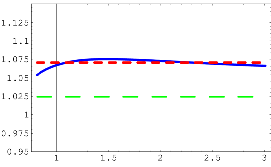
Figure 4: The solid line denotes $r(M^{2},\varrho,s)$ for the best-fitted parameters $\varrho=1.1,~{}s_{0}=3.24$. The short-dashed line corresponds to the value $r=1.07$, whereas the long-dashed line corresponds to $r$ calculated with $\Lambda_{3}=200$ MeV.

for the standard value of the gluon condensate $\langle{G^{2}}\rangle\equiv\langle{\alpha_{s}GG}\rangle/\pi=0.012~{}{\text{GeV}^{4}}$, SVZ , and with the fitting parameters, i.e., the coupling to the $\pi^{\prime}$, $\varrho\approx 1.1$, and the duality interval $s_{0}=3.24~{}{\text{GeV}^{2}}$ yields

$$\ r=1.07(\pm 0.01)\Rightarrow\delta^{2}\approx 0.19~{}{\text{GeV}^{2}}~{}\mbox{for }~{}\Lambda_{3}^{\text{LO}}=0.312~{}{\text{MeV}}\,.$$ (A.3)

The stability of the SR (A.2) with respect to the Borel parameter $M^{2}$ is rather good, as the solid line in Fig. 4 clearly effects.

Note that adopting the popular option $\Lambda_{3}^{\text{LOpop}}=200$ MeV, it simply imitates the $\alpha_{s}^{\text{NLO}}(\mu^{2})$ behavior at intermediate scales $\mu^{2}$, providing $r=1.02(\pm 0.01)$ and $\delta^{2}\approx 0.20~{}{\text{GeV}^{2}}$. This old estimate OPiv88 is also presented here for comparison (cf. long-dashed line in Fig. 4). The parameter $r$ is also rather sensitive to the value of $\langle{G^{2}}\rangle$. For example, the new estimate of the mean value $\langle{G^{2}}\rangle=0.009~{}{\text{GeV}^{4}}$, suggested quite recently in Ioffe02 , leads to $r\simeq 1.1$ and $\delta^{2}\simeq 0.18~{}{\text{GeV}^{2}}$. Taking into account the last estimate, we derive the uncertainty $\Delta_{G}\delta^{2}\simeq 0.01~{}{\text{GeV}^{2}}$. The other uncertainties, inherent in the SR method (A.2), result to an overall effect of the same order: viz., $\Delta\delta^{2}\simeq 0.01~{}{\text{GeV}^{2}}$. Finally, we can establish for $\delta^{2}$ an accuracy: $\delta^{2}=(0.19\pm 0.02)~{}{\text{GeV}^{2}}$ for $\lambda_{q}^{2}=0.4~{}{\text{GeV}^{2}}$.

In the same way we obtain from (A.1) the corresponding central values and uncertainties of $\delta^{2}$ for the higher value of $\lambda_{q}^{2}=0.5~{}{\text{GeV}^{2}}$ ($\delta^{2}=0.235\pm 0.025$) and analogously for the trial value $\lambda_{q}^{2}=0.6~{}{\text{GeV}^{2}}$ ($\delta^{2}=0.29\pm 0.03~{}{\text{GeV}^{2}}$), the latter being of interest due to instanton models  DEM97 ; Pra01 .

The one-loop anomalous dimension of $\delta^{2}$ is $\gamma_{T4}=32/9$ (see, for instance, BKM00 ). On the other hand, the one-loop scale dependence of $\delta^{2}(\mu^{2})$ is given by

$$\delta^{2}(\mu^{2})=\left[\frac{\alpha_{s}(\mu^{2})}{\alpha_{s}(\mu^{2}_{0})}\right]^{\gamma_{T4}/b_{0}}\delta^{2}(\mu^{2}_{0})\,.$$ (A.4)

Appendix B CZ DA normalization point

The authors of SchmYa99 used as a normalization point for the CZ DA the scale $\mu_{1}^{2}=0.5~{}{\text{GeV}^{2}}$, which is significantly larger than the original one used by Chernyak and Zhitnitsky: $\mu_{\text{CZ}}^{2}=0.25~{}{\text{GeV}^{2}}$. This latter and rather low normalization point is due to the fact that CZ employed the description of charmonium decays, where the characteristic virtuality of the pion is indeed of this low order as $\mu^{2}_{\text{CZ}}$. Furthermore, in order to construct their model at such a low scale, they evolved the 2nd moments, determined at a scale of 1.5 GeV², down to this scale using 1-loop evolution equations with $\Lambda_{\text{QCD}}=100~{}{\text{MeV}}$. The result is the well-known CZ DA:

$$\varphi_{\text{CZ}}(x;\mu_{\text{CZ}}^{2})=6x(1-x)\left[1+\frac{2}{3}C^{3/2}_{2}(2x-1)\right]=30x(1-x)(1-2x)^{2}\,.$$ (B.1)

However, if one wants to know the shape of this model at another scale, one has to evolve it to that scale. But a natural question arises: what evolution equation should be used to do that?

From our point of view, the best solution would be to determine once and for all the value of the second Gegenbauer coefficient of the CZ DA at the standard QCD SR scale, $\mu_{0}^{2}=1~{}{\text{GeV}^{2}}$, which is, also according to the CZ arguments, rather close to the scale of the second moment, 1.5 GeV². In this sort of determination, one needs to evolve from the CZ scale $\mu_{\text{CZ}}^{2}$ to the scale $M^{2}=1.5~{}{\text{GeV}^{2}}$ of the second moment $\langle{\xi^{2}}\rangle_{\text{CZ}}$ using the same 1-loop evolution equations (with $\Lambda_{\text{QCD}}=100~{}{\text{MeV}}$) as in their original paper CZ82 . This produces

$$a_{2}^{\text{CZ}}(\mu^{2}=1.5~{}{\text{GeV}^{2}})=0.51\,.$$ (B.2)

But after restoring this way the CZ model at a scale of 1.5 GeV², we should use for the evolution to 1 GeV² the actual value of the 1-loop QCD scale, i.e., 312 MeV. This gives

$$a_{2}^{\text{CZ}}(\mu^{2}=1~{}{\text{GeV}^{2}})=0.56\,.$$ (B.3)

Appendix C Radiative corrections

C.1 Structure of the NLO amplitude $\mathbf{T_{1}}(Q^{2},q^{2};\mu^{2};x)$

Here we present diagram per diagram the results of the NLO $T_{1}$ calculation, performed in KMR86 in the Feynman gauge using the “naive-$\gamma_{5}$ scheme” DaCh81 ; MNP01a .

Table 4: NLO results for individual diagrams⁶

	$\vphantom{{}^{\Big{|}}_{\Big{|}}}T_{1}=N_{T}\big{[}\log$-part $+\ C_{1}\big{]}$
Diagram	ln[¯Q^2/μ^2 ]-part	C_1(x,ω)
	$\displaystyle\ln\Big{[}\frac{\bar{Q}^{2}}{\mu_{F}^{2}}\Big{]}C_{0}(u,\omega)\mathop{\otimes}\limits_{u}V_{a}(u,x)_{+}$ $\displaystyle+\ \ln\Big{[}\frac{\bar{Q}^{2}}{\mu_{F}^{2}}\Big{]}C_{0}(x,\omega)~{}~{}~{}~{}~{}~{}~{}~{}~{}~{}~{}~{}$	$$C^{\prime}_{0}(u,\omega)\mathop{\otimes}\limits_{u}V_{a}(u,x)_{+}\ +\ C^{\prime}_{0}(x,\omega)$$
	$\displaystyle\ln\Big{[}\frac{\bar{Q}^{2}}{\mu_{F}^{2}}\Big{]}C_{0}(u,\omega)\mathop{\otimes}\limits_{u}V_{b}(u,x)_{+}$ $\displaystyle-\ 2\ln\Big{[}\frac{\bar{Q}^{2}}{\mu_{R}^{2}}\Big{]}C_{0}(x,\omega)~{}~{}~{}~{}~{}~{}~{}~{}~{}~{}$	$\displaystyle\Big{[}C^{\prime}_{0}(u,\omega)-C_{0}(u,\omega)\Big{]}\mathop{\otimes}\limits_{u}V_{b}(u,x)_{+}-\ 2C_{0}(x,\omega)$ $\displaystyle+\ \Big{\{}\ln[1+\omega(\bar{u}-u)]\mathop{\otimes}\limits_{u}\frac{V_{b}(u,x)_{+}+K(u,x)}{\bar{Q}^{2}[1+\omega(\bar{x}-x)]}$ $\displaystyle+\ (x\to\bar{x})\Big{\}}~{}~{}~{}~{}~{}~{}~{}~{}~{}~{}~{}~{}~{}~{}~{}~{}~{}~{}~{}~{}~{}~{}~{}~{}~{}~{}~{}~{}~{}~{}~{}~{}~{}~{}~{}$
	$$\ln\Big{[}\frac{\bar{Q}^{2}}{\mu_{R}^{2}}\Big{]}C_{0}(x,\omega)$$	$$C^{\prime}_{0}(x,\omega)-C_{0}(x,\omega)$$

To make the presentation more compact, the average virtuality $\bar{Q}^{2}$ and the asymmetry parameter $\omega$

$$\bar{Q}^{2}=\frac{Q^{2}+q^{2}}{2}\,,~{}~{}~{}\omega=\frac{Q^{2}-q^{2}}{Q^{2}+q^{2}}\,,$$ (C.1)

have been used, employing also the notation $\bar{x}\equiv 1-x$.

The results are expressed in terms of the LO coefficient function $C_{0}(x,\omega)$ (see Eq. (4)) and its logarithmic modification $C^{\prime}_{0}(x,\omega)$, naturally appearing in NLO calculations,

$$C_{0}(x,\omega)=\frac{1}{\bar{Q}^{2}}\frac{1}{1+\omega(\bar{x}-x)}+(x\to\bar{x})\,;~{}~{}~{}C^{\prime}_{0}(x,\omega)=\frac{1}{\bar{Q}^{2}}\frac{\ln[1+\omega(\bar{x}-x)]}{1+\omega(\bar{x}-x)}+(x\to\bar{x}),$$ (C.2)

and their convolutions with $V_{a}$ and $V_{b}$, the latter being parts of the LO ERBL kernel,

$$V_{a}(y,x)=2C_{\text{F}}\,\theta(x-y)\frac{y}{x}+(x\to\bar{x},y\to\bar{y})\,;~{}~{}V_{b}(y,x)=2C_{\text{F}}\,\frac{y}{x}\frac{\theta(x-y)}{x-y}+(x\to\bar{x},y\to\bar{y})\,;$$

$$V_{0}(y,x)=V_{a}(y,x)_{+}+V_{b}(y,x)_{+}=2C_{\text{F}}\left[\theta(x-y)\frac{y}{x}\left(1+\frac{1}{x-y}\right)+(x\to\bar{x},y\to\bar{y})\right]_{+}\,.$$ (C.3)

Here, the ₊-form of a distribution $V(y,x)$ is defined in the common way:

$$V(y,x)_{+}\equiv V(y,x)-\delta(y-x)\int_{0}^{1}V(u,x)\,du\,.$$ (C.4)

The expression for diagram b) requires a more complicated construction involving $K$:

$$K(y,x)=C_{\text{F}}\,\theta(x-y)\frac{1}{x}-(x\to\bar{x},y\to\bar{y})\,.$$ (C.5)

The $\log$ terms, containing the ultraviolet scale $\mu_{\text{R}}^{2}$ in Table 4, are completely cancelled out on account of additional diagrams with self-energy corrections to the quark legs DaCh81 , with contributions of the form $\ln(\mu_{F}^{2}/\mu_{R}^{2})\cdot C_{0}(x,\omega)$. The cancellation of the $\ln(\mu_{\text{R}}^{2})$ terms for the full set of diagrams is a consequence of the Ward identity in QED. Finally, collecting the $\log$ terms from all diagrams, one obtains $\ln(\bar{Q}^{2}/\mu_{F}^{2})\cdot C_{0}\otimes V_{0}$ in accordance with Eq. (5).

To perform the (formal) limit $q^{2}\to 0$ in (5), one has to take $\omega\to 1$ in the formulas of Table 4, giving rise to the known expression for $T_{1}$ DaCh81 ; KMR86 , MNP01a :

$$T(Q^{2},0;\mu_{\text{F}}^{2};x) \!\!=\!\! \frac{N_{T}}{Q^{2}}\left\{\frac{1}{x}+\frac{\alpha_{s}(\mu_{\text{R}}^{2})}{4\pi}\left[\ln\left(\frac{Q^{2}}{\mu_{\text{F}}^{2}}\right)\frac{1}{u}\mathop{\otimes}\limits_{u}V_{0}(u,x)+\frac{C_{\text{F}}}{x}\left(\ln^{2}x-\frac{x\ln x}{1-x}-9\right)\right]\right\}$$ (C.6)

$$+\ (x\to\bar{x})\ +\ {\cal O}\Big{(}\frac{1}{Q^{4}}\Big{)}\,;$$

$$C_{1}(Q^{2},0;x) = \frac{C_{\text{F}}}{xQ^{2}}\left(\ln^{2}x-\frac{x\ln x}{1-x}-9\right)\ +\ (x\to\bar{x}),$$ (C.7)

At the scale $\mu_{\text{F}}^{2}=\mu_{\text{R}}^{2}=Q^{2}$, this leads to

$$Q^{2}F^{\gamma^{*}\gamma\pi}(Q^{2},0)=\sqrt{2}f_{\pi}\left[1+\tilde{a}_{2}+\tilde{a}_{4}+\frac{\alpha_{s}(Q^{2})C_{\text{F}}}{4\pi}\left(-5+\tilde{a}_{2}h_{2}+\tilde{a}_{4}h_{4}\right)-\frac{\delta(Q^{2})}{Q^{2}}\frac{80}{27}\right];$$ (C.8)

$$h_{n}\equiv\frac{1}{3}Q^{2}C_{1}(Q^{2},0;x)\mathop{\otimes}\limits_{x}\psi_{n}(x)\,;\quad h_{2}=\frac{295}{72}\,;\quad h_{4}=\frac{10487}{900}\,,$$ (C.9)

where $\tilde{a}_{n}=a_{n}^{\text{RG}}(Q^{2})$ and $h_{n}$ gives the size of the leading radiative corrections to the contribution of the $n$th Gegenbauer eigenfunctions $\psi_{n}(x)$, entering the expansion of $\varphi_{\pi}(x)$ (see Eq. (8)).

C.2 NLO coupling constant

Let us start with the RG equation for the rescaled running coupling $\displaystyle a_{s}\left(Q^{2}\right)\equiv\alpha_{s}(Q^{2})\left(\frac{b_{0}(N_{f})}{4\pi}\right)$:

$$\frac{da_{s}\left(Q^{2}\right)}{d\ln(Q^{2})}=\bar{\beta}\left(a_{s}(Q^{2}),N_{f}\right)\,,$$ (C.10)

where $N_{f}$ is the number of active flavors and the modified $\bar{\beta}$-function reads

$$\bar{\beta}\left(a_{s},N_{f}\right)=-a_{s}^{2}\left(1+c_{1}a_{s}+c_{2}a_{s}^{2}+\ldots\ \right)\,,$$ (C.11)

with $\displaystyle c_{k}\equiv c_{k}\left(N_{f}\right)=\frac{b_{k}\left(N_{f}\right)}{b_{0}\left(N_{f}\right)^{k+1}}$, and the standard $\beta$-function coefficients are given by

$$b_{0}\left(N_{f}\right) = \frac{11N_{c}-2N_{f}}{3}\,;$$ (C.12)

$$b_{1}\left(N_{f}\right) = \frac{34}{3}N_{c}^{2}-\left(2C_{\text{F}}+\frac{10}{3}N_{c}\right)N_{f}\,;$$ (C.13)

$$b_{2}\left(N_{f}\right) = \frac{2857}{2}-\frac{5033}{18}N_{f}+\frac{325}{54}N_{f}^{2}\,.$$ (C.14)

Following here SY, we use the strong coupling constant in Sec. III in a “Particle Data Group” (PDG) form, which is the expanded second-order iteration of the 2-loop equation (C.10):

$$\alpha_{s}^{\text{PDG}}\left(Q^{2},N_{f}\right)=\frac{4\pi}{b_{0}\left(N_{f}\right)L(Q^{2})}\left[1-\frac{L_{1}(Q^{2})}{L(Q^{2})}+\ \frac{L_{1}(Q^{2})^{2}-c_{1}L_{1}(Q^{2})-c_{12}}{L(Q^{2})^{2}}\right]\,$$ (C.15)

with

$$L(Q^{2})\equiv\ln\left[\frac{Q^{2}}{\Lambda\left(N_{f}\right)^{2}}\right];\,L_{1}(Q^{2})\equiv c_{1}\ln\left[L(Q^{2})\right];\,c_{12}\equiv c_{1}^{2}-c_{2}\,,$$ (C.16)

where we fixed $\Lambda_{5}=\Lambda\left(N_{f}=5\right)$ with the help of PDG2000

$$\alpha_{s}\left(Q^{2}=(91.2\ {\text{GeV}})^{2},N_{f}=5\right)=0.118\,.$$ (C.17)

Matching this coupling at the $N_{f}=4$ threshold, $Q_{4}=10\ {\text{GeV}}$, and analogously at the $N_{f}=3$ threshold, $Q_{3}=2.4\ {\text{GeV}}$, we arrive at

$$\Lambda_{3}=380\ {\text{MeV}}\ .$$ (C.18)

But one can (we actually did this already in Sec. IV) use instead the exact solution of the 2-loop RG equation, rather than the PDG-booklet expression. This exact solution can be expressed in terms of the quantity $a_{s}$ to read

$$\frac{1}{a_{s}(Q^{2})}-c_{1}\ln\left[\frac{1}{a_{s}(Q^{2})}+c_{1}\right]=L(Q^{2})\,.$$ (C.19)

As has been shown in Mag98 the two-loop running coupling in QCD, being the solution of this equation, can be written via the Lambert $W$ function:

$$\alpha_{s}^{\text{2-loop}}\left(Q^{2},N_{f}\right)=-\frac{4\pi}{b_{0}\left(N_{f}\right)c_{1}}\left(1+W\left\{-\frac{1}{c_{1}}\left[\frac{\Lambda^{2}(N_{f})}{eQ^{2}}\right]^{1/c_{1}}\right\}\right)^{-1}\,.$$ (C.20)

The difference between the PDG form and the exact solution varies from 3.5% at $Q^{2}=10$ GeV² to 18% at $Q^{2}=1$ GeV² when one uses the same value of $\Lambda=380$ MeV for both functions. In a real situation, the values of $\Lambda$ in the two cases are different and are fixed in accordance with the standard boundary condition (C.17), so that $\Lambda_{3}^{\text{PDG}}=380$ MeV and $\Lambda_{3}^{\text{2-loop}}=408$ MeV. The deviation between the two forms becomes less pronounced at higher $Q^{2}$ and varies from 0.7% at $Q^{2}=10$ GeV² to 10% at $Q^{2}=1$ GeV² – see Fig. 5.

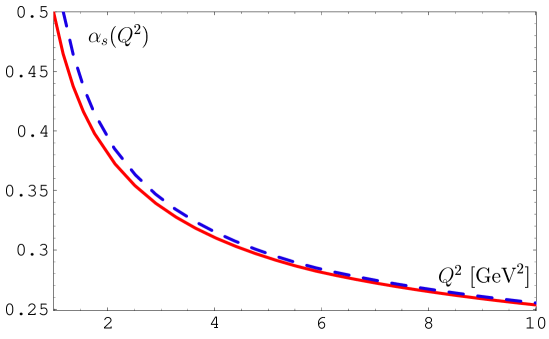
Figure 5: $Q^{2}$-dependence of two different 2-loop running couplings, $\alpha_{s}^{\text{2-loop}}(Q^{2})$ and $\alpha_{s}^{\text{PDG}}(Q^{2})$: the solid line corresponds to the exact solution of the RG-equation, Eq. (C.20); the dashed line to the PDG-booklet approximate form, Eq. (C.15).

It should be realized from this comparison that the PDG formula (C.15) is afflicted by a large error at $Q^{2}=1~{}{\text{GeV}^{2}}$ and for that reason it is preferable in the low $Q^{2}$-region ($\leq 2~{}{\text{GeV}^{2}}$) to use the exact formula (C.20). It is worth to note here that in the case of treating the heavy-quark thresholds in a more accurate way, as done in SM94 , the deviation between the PDG expression and the exact formula for the strong coupling becomes lower – at $Q^{2}=1~{}{\text{GeV}^{2}}$ about 5%.

Appendix D The NLO evolution of DA

The ERBL evolution equation and its kernel have, respectively, the following structure (for more details, see, for example, Ste99 )

$$\frac{d\,\varphi_{\pi}(x;\mu^{2})}{d\,\ln\mu^{2}} = V(x,u;\alpha_{s}(\mu^{2}))\mathop{\otimes}\limits_{u}\varphi_{\pi}(u;\mu^{2})\,;$$ (D.1)

$$V(x,u;\alpha_{s}) = \left(\frac{\alpha_{s}}{4\pi}\right)V_{0}(x,y)+\left(\frac{\alpha_{s}}{4\pi}\right)^{2}V_{1}(x,y)+\ldots$$ (D.2)

Its eigenvalues $\gamma_{n}(\alpha_{s})$ and eigenfunctions $\Psi_{n}(x;\alpha_{s})$ are defined through

$$V(x,u;\alpha_{s})\mathop{\otimes}\limits_{u}\Psi_{n}(u;\alpha_{s}) = \gamma_{n}(\alpha_{s})\Psi_{n}(x;\alpha_{s})\,.$$ (D.3)

We use the following notations for its eigenvalues Ynd83

$$\gamma_{n}(\alpha_{s}) = -\frac{1}{2}\left[\left(\frac{\alpha_{s}}{4\pi}\right)\gamma_{0}(n)+\left(\frac{\alpha_{s}}{4\pi}\right)^{2}\gamma_{1}(n)+\ldots\right]\,,$$ (D.4)

where the sign “$-$” just allows one to work with positive numbers $\gamma_{0}(n)$ and $\gamma_{1}(n)$:

$$\gamma_{0}(0) = 0,\quad\quad\quad\gamma_{1}(0)\ =\ 0\,,$$ (D.5)

$$\gamma_{0}(2) = \frac{100}{9},\quad\quad\gamma_{1}(2)\ =\ \frac{34450}{243}-\frac{830}{81}N_{f}\,,$$ (D.6)

$$\gamma_{0}(4) = \frac{728}{45},\quad\quad\gamma_{1}(4)\ =\ \frac{662846}{3375}-\frac{31132}{2025}N_{f}\,.$$ (D.7)

The two-loop eigenfunctions $\Psi_{n}^{\text{2-loop}}(x;\alpha_{s})$ of the ERBL equation (D.1) can be expanded in terms of the one-loop eigenfunctions $\psi_{n}(x)$ (see Eq. (8)). The approximate solution (6) in NLO is then given by

$$\varphi_{\pi}^{\text{RG}}(x,\mu^{2}) = \sum\limits_{n}a_{n}(\mu_{0}^{2})E(n,\mu^{2})\left[\psi_{n}(x)+\frac{\alpha_{s}(\mu)}{4\pi}\sum\limits_{k>n}d_{nk}(\mu^{2},\mu_{0}^{2})\psi_{k}(x)\right]\,,$$ (D.8)

$$E(n,\mu^{2}) \equiv \exp\left[\int\limits_{a_{s}(\mu_{0}^{2})}^{a_{s}(\mu^{2})}\frac{\gamma_{n}(4\pi a/b_{0})\ da}{\bar{\beta}(a)}\right]\,,$$ (D.9)

with $a_{0}=1$, see, e.g., MR86 . The “diagonal” part (in the $\{\psi_{n}\}$ basis) of (D.8), expressed by the standard RG exponent, is the exact part of this solution, while the “non-diagonal” part is taken in the NLO approximation. The coefficients $d_{nk}(\mu^{2},\mu_{0}^{2})$, corresponding to the non-diagonal part, fix the mixing of the higher harmonics, $k>n$, due to the fact that the matrix of the anomalous dimensions is triangular in the $\{\psi_{n}\}$ basis. The exponent $E(n,\mu^{2})$ in (D.8) can be written explicitly (the scale $\mu_{0}^{2}$ can be fixed at some arbitrary value $\simeq 1\text{ GeV}^{2}$) to read

$$E(n,Q^{2}) = \left[\frac{a_{s}(Q^{2})}{a_{s}(\mu^{2}_{0})}\right]^{\frac{\gamma_{0}(n)}{2b_{0}}}\left[\frac{1+c_{1}a_{s}(Q^{2})}{1+c_{1}a_{s}(\mu^{2}_{0})}\right]^{\omega(n)},$$ (D.10)

$$\omega(n) \equiv \frac{\gamma_{1}(n)b_{0}-\gamma_{0}(n)b_{1}}{2b_{0}b_{1}}\,.$$ (D.11)

Evolving according to (D.8), the Gegenbauer coefficients $a_{2},a_{4}$ change from the scale $\mu^{2}_{0}=\mu^{2}_{\text{SY}}$ to the scale $Q^{2}$ as follows

$$a_{2}\to U_{2}(Q^{2},a_{2})=a_{2}E(2,Q^{2})+\frac{\alpha_{s}(Q^{2})}{4\pi}d_{02}(Q^{2},\mu^{2}_{0})\,,$$ (D.12)

$$a_{4}\to U_{4}(Q^{2},a_{2},a_{4})=a_{4}E(4,Q^{2})+\frac{\alpha_{s}(Q^{2})}{4\pi}\left[d_{04}(Q^{2},\mu^{2}_{0})\right.$$

$$\phantom{a_{4}\to U_{4}(Q^{2},a_{2},a_{4})=}+\left.a_{2}E(2,Q^{2})d_{24}(Q^{2},\mu^{2}_{0})\right].$$ (D.13)

Here the NLO mixing coefficients are ($k=2,4\geq n=0,2$)

$$d_{nk}(Q^{2},\mu^{2}) = \frac{M_{nk}}{\gamma_{0}(k)-\gamma_{0}(n)-2b_{0}}\left\{1-\left[\frac{\alpha_{s}(Q^{2})}{\alpha_{s}(\mu^{2})}\right]^{[\gamma_{0}(k)-\gamma_{0}(n)]/(2b_{0})-1}\right\}\,,$$ (D.14)

where the values of the first few elements of the matrix $M_{nk}$ are

$$M_{02}=-11.2+1.73N_{f},~{}~{}M_{04}=-1.41+0.565N_{f},~{}~{}M_{24}=-22.0+1.65N_{f}\,.$$ (D.15)

Analytic expressions for $M_{nk}$ have been obtained in Mul94 . Using them one can estimate that the accuracy of (D.15) is of the order of 1%.

One appreciates from Eq. (D.8) that the NLO evolution inevitably generates higher harmonics. Even in our case, where we have as a starting point only two harmonics $a_{2}(\mu_{0}^{2})\neq 0$ and $a_{4}(\mu_{0}^{2})\neq 0$, the evolution to the scale $Q^{2}$ produces $a_{k}(Q^{2})\neq 0$ for all $k\geq 6$. As one can see from Eq. (D.8), for $k\geq 6$ these harmonics are of NLO ($a_{k}(Q^{2})\sim\alpha_{s}(Q^{2})$). For this reason and owing to the enormous computional efforts needed for this task, we take into account only the complete NLO evolution of the first two nontrivial harmonics.

Appendix E Expressions for the NLO LCSR transition form factor

We employ a similar formalism as that used in Kho99 ; SchmYa99 . However, to make the present investigation self-contained, we provide explicit expressions, given also that the formulas provided in SchmYa99 are actually incomplete and only partially contained in Kho99 . All in all, the NLO LCSR transition form factor is

$$F_{\pi\gamma^{*}\gamma}(M^{2},Q^{2},a_{2},a_{4}) = F_{\pi\gamma^{*}\gamma}^{\textsc{LO}}(M^{2},Q^{2},a_{2},a_{4})+\frac{\alpha_{s}(Q^{2})C_{\text{F}}}{2\pi}\ F_{\pi\gamma^{*}\gamma}^{\textsc{NLO}}(M^{2},Q^{2},a_{2},a_{4})$$ (E.1)

$$+ F_{\pi\gamma^{*}\gamma}^{\textsc{Tw-4}}(M^{2},Q^{2})$$

with

$$F_{\pi\gamma^{*}\gamma}^{\textsc{(N)LO}}(M^{2},Q^{2},a_{2},a_{4}) = \frac{\sqrt{2}f_{\pi}}{3}\left[G_{0}^{\textsc{(N)LO}}(Q^{2},M^{2})+U_{2}(Q^{2},a_{2})G_{2}^{\textsc{(N)LO}}(Q^{2},M^{2})\right.$$

$$\qquad\quad+\left.U_{4}(Q^{2},a_{2},a_{4})G_{4}^{\textsc{(N)LO}}(Q^{2},M^{2})\right]\,,$$

$$F_{\pi\gamma^{*}\gamma}^{\textsc{Tw-4}}(M^{2},Q^{2})=\frac{\sqrt{2}f_{\pi}}{3}\left[\frac{1}{m_{\rho}^{2}}\int_{0}^{s_{0}}\rho^{\textsc{Tw-4}}(Q^{2},S)e^{\frac{m_{\rho}^{2}-S}{M^{2}}}dS+\frac{1}{Q^{2}}H^{\textsc{Tw-4}}(Q^{2})\right]\,,$$ (E.2)

where the evolution functions $U_{2}(Q^{2},a_{2})$ and $U_{4}(Q^{2},a_{2},a_{4})$ are described in Appendix D. We also define the following LCSR functions

$$Q^{2}G_{k}^{\textsc{order}}(Q^{2},M^{2}) = \frac{Q^{2}}{m_{\rho}^{2}}\int_{0}^{s_{0}}\rho_{k}^{\textsc{order}}(Q^{2},S)e^{\frac{m_{\rho}^{2}-S}{M^{2}}}dS+H_{k}^{\textsc{order}}(Q^{2})\,;$$ (E.3)

$$H_{k}^{\textsc{order}}(Q^{2}) = \int_{s_{0}}^{\infty}\rho_{k}^{\textsc{order}}(Q^{2},S)\frac{Q^{2}dS}{S}\,;$$ (E.4)

$$H^{\textsc{Tw-4}}(Q^{2}) = \int_{s_{0}}^{\infty}\rho^{\textsc{Tw-4}}(Q^{2},S)\frac{Q^{2}dS}{S}\,,$$ (E.5)

for $k=0,2,4$ and set order$=$ LO or NLO. The spectral densities in LO are

$$\rho_{0}^{\textsc{LO}}(u,s) = \frac{6us}{(u+s)^{3}}\,;$$ (E.6)

$$\rho_{2}^{\textsc{LO}}(u,s) = \frac{36us(u^{2}-3us+s^{2})}{(u+s)^{5}}\,;$$ (E.7)

$$\rho_{4}^{\textsc{LO}}(u,s) = \frac{90us(u^{4}-10u^{3}s+20u^{2}s^{2}-10us^{3}+s^{4})}{(u+s)^{7}}$$ (E.8)

and in NLO (see SchmYa99 ) —

$$\rho_{0}^{\textsc{NLO}}(u,s) = \frac{-us}{(u+s)^{3}}\left[15-\pi^{2}+3\left(\ln\frac{s}{u}\right)^{2}\right]\,;$$ (E.9)

$$\rho_{2}^{\textsc{NLO}}(u,s) = \frac{-s}{4(u+s)^{5}}\left[\vphantom{\frac{s}{u}}25s^{3}-8(95+3\pi^{2})s^{2}u+36(25+2\pi^{2})su^{2}-12(5+2\pi^{2})u^{3}\right.$$ (E.10)

$$\left.~{}~{}~{}~{}~{}~{}~{}~{}~{}~{}~{}~{}~{}~{}+12(s^{2}-3su+u^{2})u\ln\frac{s}{u}\left(25+6\ln\frac{s}{u}\right)\right]\,;$$

$$\rho_{4}^{\textsc{NLO}}(u,s) = \frac{-s}{10(u+s)^{7}}\left[\vphantom{\frac{s}{u}}91s^{5}-2(5413+75\pi^{2})s^{4}u+125(541+12\pi^{2})s^{3}u^{2}\right.$$ (E.11)

$$\left.~{}~{}~{}~{}~{}~{}~{}~{}~{}~{}~{}~{}~{}~{}~{}-100(901+30\pi^{2})s^{2}u^{3}+150(193+10\pi^{2})su^{4}\right.$$

$$\left.~{}~{}~{}~{}~{}~{}~{}~{}~{}~{}~{}~{}~{}~{}~{}-15(109+10\pi^{2})u^{5}+30(s^{4}-10s^{3}u+20s^{2}u^{2}-10su^{3}+u^{4})u\right.$$

$$\left.~{}~{}~{}~{}~{}~{}~{}~{}~{}~{}~{}~{}~{}~{}~{}~{}~{}~{}~{}~{}~{}~{}~{}~{}~{}~{}~{}~{}~{}~{}~{}~{}~{}~{}~{}~{}~{}~{}~{}~{}~{}~{}~{}~{}~{}~{}\times\ln\frac{s}{u}\left(91+15\ln\frac{s}{u}\right)\right]\,.$$

Contributions from higher states in LO are given by

$$H_{0}^{\textsc{LO}}(u) = \frac{3u^{2}}{(u+s_{0})^{2}}\,;$$ (E.12)

$$H_{2}^{\textsc{LO}}(u) = \frac{3u^{2}(u^{2}-8us_{0}+6s_{0}^{2})}{(u+s_{0})^{4}}\,;$$ (E.13)

$$H_{4}^{\textsc{LO}}(u) = \frac{3u^{2}(u^{4}-24u^{3}s_{0}+90u^{2}s_{0}^{2}-80us_{0}^{3}+15s_{0}^{4})}{(u+s_{0})^{6}}$$ (E.14)

and in NLO:

$$H_{0}^{\textsc{NLO}}(u) = \frac{-15{u^{2}}}{2(u+s_{0})^{2}}-\frac{3s_{0}}{(u+s_{0})}\ln\frac{s_{0}}{u}+\frac{3(2u+s_{0})s_{0}}{2(u+s_{0})^{2}}\left[\left(\ln\frac{s_{0}}{u}\right)^{2}-\frac{\pi^{2}}{3}\right]$$ (E.15)

$$- 3\left[\textbf{Li}_{2}\left(-\frac{s_{0}}{u}\right)-\left(1-\ln\frac{s_{0}}{u}\right)\ln(1+\frac{s_{0}}{u})\right]\,;$$

$$H_{2}^{\textsc{NLO}}(u) = \frac{5{u}}{48(u+s_{0})^{4}}\left(59{u^{3}}-352{u^{2}}{s_{0}}+564{u}{s_{0}^{2}}-72{s_{0}}^{3}\right)$$ (E.16)

$$+ \frac{3s_{0}}{2(u+s_{0})^{4}}\left(12u^{3}+4u{s_{0}}^{2}+{s_{0}}^{3}\right)\left[\left(\ln\frac{s_{0}}{u}\right)^{2}-\frac{\pi^{2}}{3}\right]$$

$$+ \frac{1}{4(u+s_{0})^{4}}\left(5{u^{4}}+4{s_{0}}\left(47{u^{3}}-3{s_{0}}\left(18{u^{2}}+3u{s_{0}}+{s_{0}}^{2}\right)\right)\right)\ln\frac{s_{0}}{u}$$

$$- 3\left[\textbf{Li}_{2}\left(-\frac{s_{0}}{u}\right)-\left(1-\ln\frac{s_{0}}{u}\right)\ln(1+\frac{s_{0}}{u})\right]+\frac{5}{4}\ln(1+\frac{u}{s_{0}})\,;$$

$$H_{4}^{\textsc{NLO}}(u) = \frac{u}{600(u+s_{0})^{6}}\left(\vphantom{\frac{s_{0}}{u}}10487{u^{5}}-149418{u^{4}}{s_{0}}+678285{u^{3}}{s_{0}}^{2}-888520{u^{2}}{s_{0}}^{3}\right.$$ (E.17)

$$\left.\vphantom{\frac{s_{0}}{u}}~{}~{}~{}~{}~{}~{}~{}~{}~{}~{}~{}~{}~{}~{}~{}~{}+259260{u}{s_{0}}^{4}-6300{s_{0}}^{5}\right)$$

$$+ \frac{3{s_{0}}}{2(u+{s_{0}})^{6}}\left(30{u^{5}}-75{u^{4}}{s_{0}}+100{u^{3}}{s_{0}}^{2}+6u{s_{0}}^{4}+{s_{0}}^{5}\right)\left[\left(\ln\frac{s_{0}}{u}\right)^{2}-\frac{\pi^{2}}{3}\right]$$

$$+ \frac{u}{10(u+{s_{0}})^{6}}\left(44{u^{5}}+2124{u^{4}}{s_{0}}-7575{u^{3}}{s_{0}}^{2}+8000{u^{2}}{s_{0}}^{3}\right.$$

$$\left.~{}~{}~{}~{}~{}~{}~{}~{}~{}~{}~{}~{}~{}~{}~{}~{}-1425{u}{s_{0}}^{4}+30{s_{0}}^{5}\right)\ln\frac{s_{0}}{u}-\ 3\left(\ln\frac{s_{0}}{u}\right)^{2}$$

$$- 3\left[\textbf{Li}_{2}\left(-\frac{s_{0}}{u}\right)-\left(1-\ln\frac{s_{0}}{u}\right)\ln(1+\frac{s_{0}}{u})\right]+\frac{7}{5}\ln(1+\frac{u}{s_{0}})\,.$$

The twist-four spectral density is Kho99

$$\rho^{\textsc{Tw-4}}(u,s) = \frac{80\delta^{2}(u)}{3u}\frac{2u^{2}s(s-u)}{(u+s)^{5}}\,,$$ (E.18)

where $\delta^{2}(u)$ is taken from Eq. (A.4) with $\mu^{2}=u$. This produces

$$H^{\textsc{Tw-4}}(u) = \frac{80\delta^{2}(u)}{3u}\frac{u^{3}(2s_{0}-u)}{3(u+s_{0})^{4}}\,.$$ (E.19)

References

- (1) J. Gronberg et al., Phys. Rev. D57, 33 (1998) [hep-ex/9707031].
- (2) A. Schmedding and O. Yakovlev, Phys. Rev. D62, 116002 (2000) [hep-ph/9905392].
- (3) A. Khodjamirian, Eur. Phys. J. C6, 477 (1999) [hep-ph/9712451].
- (4) A. V. Radyushkin and R. Ruskov, Nucl. Phys. B481, 625 (1996) [hep-ph/9603408].
- (5) A. P. Bakulev, S. V. Mikhailov, and N. G. Stefanis, Phys. Lett. B508, 279 (2001) [hep-ph/0103119]; in Proceedings of the 36th Rencontres De Moriond On QCD And Hadronic Interactions, 17-24 Mar 2001, Les Arcs, France [hep-ph/0104290].
- (6) A. P. Bakulev and S. V. Mikhailov, Phys. Rev. D65, 114511 (2002) [hep-ph/0203046].
-
(7)
A. V. Efremov and A. V. Radyushkin,
Phys. Lett. B94, 245 (1980);
Theor. Math. Phys. 42, 97 (1980);
G. P. Lepage and S. J. Brodsky, Phys. Lett. B87, 359 (1979); Phys. Rev. D22, 2157 (1980). -
(8)
F. del Aguila and M. K. Chase,
Nucl. Phys. B193, 517 (1981);
E. Braaten, Phys. Rev. D28, 524 (1983). - (9) E. P. Kadantseva, S. V. Mikhailov, and A. V. Radyushkin, Sov. J. Nucl. Phys. 44, 326 (1986).
- (10) I. V. Musatov and A. V. Radyushkin, Phys. Rev. D56, 2713 (1997) [hep-ph/9702443].
- (11) D. E. Groom et al., Eur. Phys. J. C15, 1 (2000).
- (12) V. M. Braun, A. Khodjamirian, and M. Maul, Phys. Rev. D61, 073004 (2000) [hep-ph/9907495].
- (13) V. L. Chernyak and A. R. Zhitnitsky, Phys. Rept. 112, 173 (1984).
- (14) M. Diehl, P. Kroll and C. Vogt, Eur. Phys. J. C22, 439 (2001) [hep-ph/0108220].
- (15) A. Khodjamirian, Nucl. Phys. B605, 558 (2001) [hep-ph/0012271].
- (16) B. Melić, B. Nižić, and K. Passek, Phys. Rev. D65, 053020 (2002) [hep-ph/0107295].
- (17) S. Dalley and B. van de Sande, hep-ph/0212086.
-
(18)
S. V. Mikhailov and A. V. Radyushkin,
Sov. J. Nucl. Phys. 49, 494 (1989);
Phys. Rev. D45, 1754 (1992);
A. P. Bakulev and S. V. Mikhailov, Phys. Lett. B436, 351 (1998). -
(19)
V. A. Novikov, M. A. Shifman, A. I. Vainshtein,
M. B. Voloshin, and V. I. Zakharov,
Nucl. Phys. B237, 525 (1984). - (20) A. A. Ovchinnikov and A. A. Pivovarov, Sov. J. Nucl. Phys. 48, 721 (1988).
- (21) A. L. Kataev, G. Parente, and A. V. Sidorov, hep-ph/0106221 (unpublished).
- (22) V. M. Belyaev and B. L. Ioffe, Sov. Phys. JETP 57, 716 (1983).
- (23) M. A. Shifman, A. I. Vainshtein, and V. I. Zakharov, Nucl. Phys. B147, 385, 448, 519 (1979).
- (24) B. L. Ioffe, hep-ph/0207191 (unpublished).
- (25) A. E. Dorokhov, S. V. Esaibegian, and S. V. Mikhailov, Phys. Rev. D56, 4062 (1997).
-
(26)
M. Praszalowicz and A. Rostworowski,
Phys. Rev. D64, 074003 (2001)
[hep-ph/0105188];
ibid. D66, 054002 (2002) [hep-ph/0111196]. - (27) V. L. Chernyak and A. R. Zhitnitsky, Nucl. Phys. B201, 492 (1982).
-
(28)
B. A. Magradze,
in Proceedings of the 10th International Seminar Quarks’98,
Suzdal, Russia, 18–24 May 1998, edited by F. L. Bezrukov et al.
(INR RAS, Moscow, 1999), pp. 158–171 [hep-ph/9808247];
E. Gardi, G. Grunberg, and M. Karliner, JHEP 07, 007 (1998) [hep-ph/9806462]. - (29) D. V. Shirkov and S. V. Mikhailov, Z. Phys. C63, 463 (1994) [hep-ph/9401270].
- (30) N. G. Stefanis, Eur. Phys. J. direct, C7, 1 (1999) [hep-ph/9911375].
- (31) F. J. Yndurin, Quantum Chromodynamics. An Introduction to the Theory of Quarks and Gluons, (Springer-Verlag, New York, Berlin, Heidelberg, Tokyo, 1983), Eq. (20.12) and (21.10).
- (32) S. V. Mikhailov and A. V. Radyushkin, Nucl. Phys. B273, 297 (1986).
- (33) D. Müller, Phys. Rev. D49, 2525 (1994); ibid. D51, 3855 (1995).