A high energy determination of Yukawa couplings
in SUSY models

Abstract

We consider the production, at future lepton colliders, of final fermion, sfermion, scalar pairs in SUSY models. For third family fermions and sfermions and for charged Higgses, the leading Yukawa effect at one loop for large c.m. energies comes from a linear logarithm of Sudakov type, that only depends, in the MSSM, on one SUSY mass scale and on $\tan\beta$. Assuming a relatively light SUSY scenario, we illustrate a possible determination of $\tan\beta$ at c.m. energies of about 1 TeV, working systematically at subleading logarithmic accuracy, at the one-loop level.

I Introduction

The possibility that virtual electroweak effects of Supersymmetric models at future lepton colliders[1, 2] can be described, for sufficiently large c.m. energies, by a logarithmic expansion of Sudakov type, has been examined in recent papers [3, 4, 5] in the simplest case of the MSSM. The first considered process has been that of final fermion pair production. This has been only treated at one-loop, computing for both massless [3] and massive [4] final states the SUSY Sudakov terms. One main conclusion is that these terms do exist and are all of ”subleading” SL (linear) kind. At one TeV, working in a relatively ”light” SUSY scenario, where the heaviest SUSY mass if of a few (two, three) hundred GeV, the numerical effects of SUSY Sudakov terms on the various observables are relatively small (a few percent at most), while at three TeV they become definitely large. The next step has been the analysis of final scalar (sfermion or Higgs) pair production for both massless and massive final states. This has been performed both at the one-loop level and at resummed subleading order accuracy [5]. By comparison of the two calculations it can be concluded that, in the assumed ”light” SUSY scenario the two approximations are practically indistinguishable at one TeV, where their effect is, as in the fermion case, relatively small, but become drastically different (and both large, well beyond a relative ten percent) in the higher (two, three TeV) energy region. Within this approach one would thus conclude that at the LC extreme energies the MSSM can be safely treated, to subleading logarithmic order accuracy, at the one loop level for what concerns fermion, sfermion, scalar Higgs production.

This conclusion could be of immediate practical consequence. In fact, it has been remarked in Refs.[4, 5] that, for production of fermions and squarks of the third family and of charged Higgs bosons, the coefficients of the SL electroweak SUSY logarithms of Yukawa origin only depend on a common SUSY scale $M_{S}$, by definition the heaviest SUSY mass involved in the electroweak component of the process, and on the ratio of the two scalar vevs $\rm tan\beta=v_{2}/v_{1}$. To the extent that a subleading order approximation can be considered as a reliable description of the variation with energy of the observables of the process, i.e. that the missing terms of the expansion can be adequately described by a constant component, this has allowed to propose a determination of $\rm tan\beta$ based on a number of measurements of the observables at different energies (roughly, on measurements of their slopes), whose main features have been already illustrated in Refs. [4, 5] in a qualitative way for fermion production and scalar production separately.

The aim of this note is that of proposing a more quantitative determination of $\rm tan\beta$ from a combined analysis of the slopes in energy of fermion, sfermion, charged Higgs production. This will be done working at the one-loop level, in an energy region around (below) 1 TeV. With this purpose, and to try to be reasonably self-consistent, we briefly recall the structure of the various Yukawa contributions in the production of pairs of fermions ($t,b$), sfermions ($\widetilde{t}_{L,R}$, $\widetilde{b}_{L,R}$) and charged Higgs in the MSSM. The complete expressions of the asymptotic contributions can be found in Refs.[4, 5], and we do not reproduce them here. Starting from them it is relatively straightforward to derive the quantities that are relevant for this note, which are given in the following list.

II Complete List of Yukawa Effects in Cross Sections and Asymmetries

We parametrize the Yukawa effects in the physical observables that we are going to analyze and summarize them by giving a complete list.

Let us denote by ${\cal O}_{n}$, the various cross sections for production of sfermions ($\widetilde{t}_{L,R}$, $\widetilde{b}_{L,R}$), charged Higgs bosons $H^{\pm}$ and third generation fermions ($t$ and $b$). For top and bottom production we also include three basic asymmetry observables (unpolarized forward-backward asymmetry $A_{FB}$, Left-Right asymmetry for longitudinally polarized $e^{\pm}$ beams $A_{LR}$ and its forward-backward asymmetry $A_{pol}$). In the case of top production the average helicity $H_{t}$ as well as its forward-backward and Left-Right asymmetries $H_{FB,t}$ and $H_{LR,t}$ should be measurable by studying the leading top decay mode $t\to Wb$. The definition of these observables, in particular of the asymmetries, is conventional and can be found in full details in Appendix B of [6].

For cross sections ${\cal O}\equiv\sigma$, we define the relative one loop SUSY effect as the ratio

$$\epsilon_{n}(q^{2})=\frac{{\cal O}_{n}(q^{2})-{\cal O}^{\rm Born+SM}_{n}(q^{2})}{{\cal O}^{\rm Born+SM}_{n}(q^{2})},$$ (1)

where “SM” denotes all the one loop terms that do not involve virtual SUSY partners (sfermions, gauginos and extra Higgs particles). For asymmetries, we consider instead the absolute SUSY effect defined as the difference

$$\epsilon_{n}(q^{2})={\cal O}_{n}(q^{2})-{\cal O}^{\rm Born+SM}_{n}(q^{2}).$$ (2)

At one loop, in the asymptotic regime, the shifts $\epsilon_{n}$ can be parametrized as

$$\epsilon(q^{2})=\frac{\alpha}{4\pi}\ F(\tan\beta)\ln\frac{q^{2}}{M_{S}^{2}}+G+{\cal O}\left(\frac{M^{2}}{q^{2}}\right),$$ (3)

where, as we wrote, $F$ is a simple function of $\tan\beta$ only. Its explicit expression must be determined by performing a Sudakov (logarithmic) expansion of the one loop calculation. The detailed analysis can be found in [3, 4, 5] and here we collect the various results for convenience of the reader.

Sfermion cross sections

$$F(\sigma_{\widetilde{t}_{L}}) = -\frac{1}{M_{W}^{2}s_{W}^{2}}\left(m_{t}^{2}\cot^{2}\beta+m_{b}^{2}\tan^{2}\beta\right),$$ (4)

$$F(\sigma_{\widetilde{t}_{R}}) = -\frac{2}{M_{W}^{2}s_{W}^{2}}\ m_{t}^{2}\cot^{2}\beta,$$ (5)

$$F(\sigma_{\widetilde{b}_{L}}) = F(\sigma_{\widetilde{t}_{L}}),$$ (6)

$$F(\sigma_{\widetilde{b}_{R}}) = -\frac{2}{M_{W}^{2}s_{W}^{2}}\ m_{b}^{2}\tan^{2}\beta$$ (7)

Charged Higgs cross section

$$F(\sigma_{H^{\pm}})=-\frac{3}{M_{W}^{2}s_{W}^{2}}\left(m_{t}^{2}\cot^{2}\beta+m_{b}^{2}\tan^{2}\beta\right).$$ (8)

Fermion cross section

$$F(\sigma_{t}) = \frac{1}{s^{2}_{W}M_{W}^{2}}\frac{1}{9-12s_{W}^{2}+88s_{W}^{4}}\times$$ (10)

$$\left(-3m_{t}^{2}(3-4s_{W}^{2}+56s_{W}^{4})\cot^{2}\beta-m_{b}^{2}(9-12s_{W}^{2}+8s_{W}^{4})\tan^{2}\beta\right)$$

$$F(\sigma_{b}) = \frac{1}{s^{2}_{W}M_{W}^{2}}\frac{1}{9-24s_{W}^{2}+40s_{W}^{4}}\times$$ (12)

$$\left(-m_{t}^{2}(9-24s_{W}^{2}+20s_{W}^{4})\cot^{2}\beta-3m_{b}^{2}(3-8s_{W}^{2}+20s_{W}^{4})\tan^{2}\beta\right)$$

Fermion cross section asymmetries

$$F(A_{FB,t}) = \frac{1}{M_{W}^{2}}\frac{72s_{W}^{2}(3-4s_{W}^{2}-4s_{W}^{4})}{(9-12s_{W}^{2}+88s_{W}^{4})^{2}}(m_{t}^{2}\cot^{2}\beta-m_{b}^{2}\tan^{2}\beta)$$ (13)

$$F(A_{LR,t}) = \frac{1}{M_{W}^{2}}\frac{384s_{W}^{2}(3-4s_{W}^{2}+s_{W}^{4})}{(9-12s_{W}^{2}+88s_{W}^{4})^{2}}(m_{t}^{2}\cot^{2}\beta-m_{b}^{2}\tan^{2}\beta)$$ (14)

$$F(A_{pol,t}) = \frac{1}{M_{W}^{2}}\frac{120s_{W}^{2}(9-12s_{W}^{2}+8s_{W}^{4})}{(9-12s_{W}^{2}+88s_{W}^{4})^{2}}(m_{t}^{2}\cot^{2}\beta-m_{b}^{2}\tan^{2}\beta)$$ (15)

$$F(A_{FB,b}) = \frac{1}{M_{W}^{2}}\frac{-18s_{W}^{2}(3-8s_{W}^{2})}{(9-24s_{W}^{2}+40s_{W}^{4})^{2}}(m_{t}^{2}\cot^{2}\beta-m_{b}^{2}\tan^{2}\beta)$$ (16)

$$F(A_{LR,b}) = \frac{1}{M_{W}^{2}}\frac{-96s_{W}^{2}(3-8s_{W}^{2}+5s_{W}^{4})}{(9-24s_{W}^{2}+40s_{W}^{4})^{2}}(m_{t}^{2}\cot^{2}\beta-m_{b}^{2}\tan^{2}\beta)$$ (17)

$$F(A_{pol,b}) = \frac{1}{M_{W}^{2}}\frac{-30s_{W}^{2}(9-24s_{W}^{2}+20s_{W}^{4})}{(9-24s_{W}^{2}+40s_{W}^{4})^{2}}(m_{t}^{2}\cot^{2}\beta-m_{b}^{2}\tan^{2}\beta)$$ (18)

Fermion helicity and its asymmetries
It has been shown in [4] that the logarithmic parts of these observables are related to those of the cross section asymmetries as follows:

$$F(H_{f}) = -\frac{4}{3}A_{pol,f}$$ (19)

$$F(H_{FB,f}) = -\frac{3}{4}A_{LR,f}$$ (20)

$$F(H_{LR,f}) = -\frac{4}{3}A_{FB,f}$$ (21)

III Limits and Confidence Regions for tan $\beta$

The constant $G$ in Eq. (3) is a sub-subleading correction that does not increase with $q^{2}$ and depends on all mass ratios of virtual particles. The omitted terms in Eq. (3) vanish in the high energy limit [7].

To eliminate $G$ we assume that a set of $N$ independent measurements is available at c.m. energies $\sqrt{q_{1}^{2}},\sqrt{q_{2}^{2}},\dots,\sqrt{q_{N}^{2}}$ and take the difference of each measurement with respect to the one at lowest energy. For each observable, the resulting quantities

$$\delta_{i}=\epsilon(q_{i}^{2})-\epsilon(q_{1}^{2}),$$ (22)

do not contain the constant term $G$ and take the simple form

$$\delta_{i}=F(\tan\beta^{*})\ \ln\frac{q_{i}^{2}}{q_{1}^{2}},$$ (23)

where $\tan\beta^{*}$ is the true unknown value that describes the experimental measurements.

We now turn to a description of a possible strategy for the determination of $\tan\beta$. It results from a non linear analysis of data that must deal with extreme situations where $\tan\beta$ is determined with a still reasonable but rather large relative error.

Let us label the various observables by the index $n=1,\dots,N_{\cal O}$ and denote by $\sigma_{n}(q^{2})$ the experimental error on $\epsilon_{n}(q^{2})$. For each set of explicit measurements $\{\delta_{n}(q_{i}^{2})\}$, the best estimate for $\tan\beta$ is the value that minimizes the $\chi^{2}$ sum

$$\chi^{2}(\tan\beta)=\sum_{i=1}^{N}\sum_{n=1}^{N_{\cal O}}\frac{[F_{n}(\tan\beta)\ln\frac{q^{2}_{i+1}}{q^{2}_{1}}-\delta_{n,i}]^{2}}{4\sigma_{n,i}^{2}},$$ (24)

where $\delta_{n,i}\equiv\delta_{n}(q^{2}_{i})$ and $\sigma_{n,i}\equiv\sigma_{n}(q_{i}^{2})$. The factor $4$ in the above formula follows from the fact that we assume a conservative error $2\sigma_{n,i}$ on the difference $\delta_{n,i}$. In other words, we describe the experimentally measured quantity $\delta_{n,i}$ in terms of a normal Gaussian random variable distributed around the theoretical value computed at $\tan\beta^{*}$

$$\delta_{n,i}=F_{n}(\tan\beta^{*})\ln\frac{q^{2}_{i+1}}{q^{2}_{1}}+2\sigma_{n,i}\ \xi_{n,i},$$ (25)

with probability density for the independent fluctuations $\{\xi_{n,i}\}$ given by

$$P(\{\xi_{n,i}\})=\prod_{n,i}\frac{1}{\sqrt{2\pi}}\ e^{-\frac{1}{2}\xi_{n,i}^{2}}.$$ (26)

In the following we shall simplify the analysis by taking a constant $\sigma_{n,i}\equiv\sigma$ with typical values around 1%. For each set of measurements we determine the optimal $\tan\beta$ that minimizes $\chi^{2}$. It is a function of the actual measurements $\{\xi_{n,i}\}$ and the width of its probability distribution $P(\tan\beta)$ determines the limits that can be assigned to the estimate of the unknown $\tan\beta^{*}$.

The distribution $P(\tan\beta)$ cannot be computed analytically because of the highly non linear dependence of the MSSM effects on $\tan\beta$. However, it can be easily obtained by Monte Carlo sampling. With this aim, we generate a large set of independent realizations of the measurements $\{\xi_{n,i}\}$ and compute for each of them $\tan\beta$. The histogram of the obtained values is a numerical estimate of the true $P(\tan\beta)$.

In previous papers [4, 5], we discussed a simplified approximate procedure and we determined the $1\sigma$ boundary on $\tan\beta$ by linearizing the dependence on $\tan\beta$ around the minimum of $\chi^{2}$. The bound that we derived is thus

$$\delta\tan\beta=2\sigma\left(\sum_{n=1}^{N_{\cal O}}F_{n}^{\prime}(\tan\beta^{*})^{2}\right)^{-1/2}\left(\sum_{i}\ln^{2}\frac{q_{i+1}^{2}}{q_{1}^{2}}\right)^{-1/2}.$$ (27)

This result can be trusted if the experimental accuracy $\sigma$ is small enough to determine a region around the minimum of $\chi^{2}$ where deviations from linearity can be neglected. It gives anyhow a rough idea of the easy regions where a determination of $\tan\beta$ from virtual one loop MSSM effects is not difficult.

In a more realistic analysis, however, this approximation can be misleading and possibly too much optimistic, especially for values of $\tan\beta$ around $15$ where the linearized analysis predicts typical relative errors around $50\%$. For this reasons, we pursue in this paper the complete Monte Carlo analysis of the allowed range of $\tan\beta$.

IV Numerical Analysis

We begin by considering the full set of 16 observables consisting in:

1. cross sections for sfermion production in the case of final $\widetilde{t}_{L}$, $\widetilde{t}_{R}$, $\widetilde{b}_{L}$, $\widetilde{b}_{L}$;

2. cross section for charged Higgs production;

3. cross sections and 3 asymmetries (forward-backward, longitudinal and polarized) for top, bottom production;

4. 3 top helicity distributions (again forward-backward, longitudinal and polarized).

We assume a set of $N=10$ measurements at energies between 600 GeV and 1 TeV with an aimed experimental precision equal to 1% for all observables at all energies. Within this ideal framework we have determined the probability distribution $P(\tan\beta)$ for $5<\tan\beta^{*}<40$. In Fig. (1) we show the associated histograms in the four cases $\tan\beta^{*}=10,15,20,25$. Even in the easiest case, $\tan\beta^{*}=25$, it is not possible to determine $\tan\beta$ in a reasonable way. There is always a rather pronounced peak at small $\tan\beta$ in the histogram and the distribution is rather broad without a second peak recognizable around the exact value.

To analyze in a quantitative way these results, we compute from each histogram the standard deviation of the estimated $\tan\beta$. If the distribution can be characterized in terms of a single dominant peak, then this is rough measure of its width. Of course, when the distribution is wide or when it is the sum of two large separated peaks, the standard deviation is a pessimistic estimate of the uncertainty on the parameter determination that can be improved by adding, for instance, some information excluding the regions corresponding to large (or small) values.

The determination of $\tan\beta$ is almost completely driven by the observables related to sfermions and charged Higgses production. In Fig. (2), we show the results obtained without observables related to top and bottom production. In Fig. (3), we show the results obtained with top, bottom and charged Higgs observables. The single measurement of charged Higgs cross section is not enough to determine $\tan\beta$ with this level of precision in the measures. Finally, in Fig. (4), we show the results obtained with sfermions and fermions observables. The single measurement of charged Higgs cross section is not enough to determine $\tan\beta$ with this level of precision in the measurements. The plot of the relative error as a function of $\tan\beta$ for the various sets of observables (including the full case) is collected in Fig. (5).

With these necessary remarks in mind, we can analyze the standard deviation of the parameter histograms and the result is shown in Fig. (5) (solid line). We see that for $\tan\beta<20$ a determination with a relative error smaller than $50\%$ is not possible.

If we consider still 10 measurements ranging from 600 GeV up to 1 TeV, but with a precision of $0.5\%$, then the scenario is quite better. In Fig. (6), we see that for $\tan\beta^{*}>20$, a well defined peak is visible in the rightmost part of the Figures roughly centered on the exact value. Fig. (10) (solid line) allows to conclude that the relative error is smaller than $50\%$ for $\tan\beta^{*}>13$ and smaller than $25\%$ for $\tan\beta^{*}>25$. Again, the role of the observables related to sparticle production is fundamental. In Fig. (7) we show what can be obtained without the information coming from top and bottom production. As one can see, there is small difference with respect to the previous two figures. Fig. (8) shows the results obtained with top, bottom and charged Higgs observables. Fig. (9) shows the results obtained with sfermions and fermions observables. Again, Fig. (10) collects the error as a function of $\tan\beta$ for the various considered cases.

As a final comment, we observe that a general feature of the histograms is the presence of a fake peak at small $\tan\beta$ as well at $\tan\beta\simeq 6$. The reason for this can be understood by analyzing what happens by exploiting in the analysis just the (dominant) charged Higgs cross section as discussed in Appendix A.

V Conclusions

In a ”standard” SUSY model, all the gauge couplings are fixed and coincide with the corresponding SM ones. For the couplings of the Yukawa sector, much more freedom is allowed. In the MSSM, one such coupling is the ratio of the scalar vevs $\tan\beta$. We have shown in this Note that, in a light SUSY scenario, a determination of $\tan\beta$ based on measurements of the slope with energy of the combined set of observables of the three processes of fermion, sfermion, scalar charged Higgs production can lead to a determination of this parameter with a relative error of 20-30 % in a range of high values that would otherwise require difficult final state analyses of Higgs decays, see the proposals in [8].

The main point of our approach is, in our opinion, the fact that in this determination $\tan\beta$ is the only SUSY parameter to be measured: all the other parameters give vanishing contributions in the high energy limit. Isolating the various SUSY parameters to be studied is in fact, in our opinion, a basic feature of any realistic ”determination strategy”.

In addition to the previous conclusion, we would like to add an extra final comment. If a SUSY model were different from the considered MSSM, in particular if it had a different Higgs structure (for example more Higgs doublets), the Yukawa couplings would be, quite generally, different. But the features of the Sudakov structure would remain essentially unchanged. This would lead to the possibility of deriving, with minor changes in our approach, the components of the SUSY Yukawa sector that dominate the high energy behaviour in this model. In analogy with what was done at LEP1 for the ”prediction”, from an analysis of one-loop effects, of the value of the top mass, that remains in our opinion one of the biggest LEP1 achievements, a combined set of high precision measurements at future linear colliders physics could therefore produce a genuine determination of this fundamental SUSY parameter.

A Analysis with the $H^{\pm}$ cross section alone

It is interesting to analyze the role of charged Higgs production in $\tan\beta$ determination when no additional observables are exploited. In fact, at the level of precision we are working, some problems arise. To see why, let us denote $\tan\beta\equiv T$ and write $\chi^{2}$ explicitly:

$$\chi^{2}(T)=\sum_{i=1}^{N}\frac{[(F(T)-F(T^{*}))\ln\frac{q^{2}_{i+1}}{q^{2}_{1}}-2\sigma\xi_{i}]^{2}}{4\sigma^{2}},$$ (A1)

The function $F(T)$ is given by

$$F(T)=-\frac{3\alpha}{4\pi M_{W}^{2}s_{W}^{2}}(m_{t}^{2}\cot^{2}\beta+m_{b}^{2}\tan^{2}\beta)$$ (A2)

If we denote $L_{i}=\log\frac{q_{i+1}^{2}}{q_{1}^{2}}$, the derivative of $\chi^{2}$ vanish when

$$F^{\prime}(T)=0\ \Rightarrow\ T=\sqrt{m_{t}/m_{b}}\simeq 6.2,$$ (A3)

and also at the solutions (if there are any) of

$$F(T)-F(T^{*})=2\sigma\frac{\sum_{i}L_{i}\xi_{i}}{\sum_{i}L_{i}^{2}},$$ (A4)

that we can write in a simpler way in terms of a new normalized gaussian random variable $\widetilde{\xi}$:

$$\Delta(T,T^{*})=\widetilde{\sigma}\ \widetilde{\xi}$$ (A5)

where

$$\Delta(T,T^{*})\equiv F(T)-F(T^{*}),\qquad\widetilde{\sigma}=\frac{2\sigma}{(\sum_{i}L_{i}^{2})^{1/2}}$$ (A6)

To discuss the solutions of Eq. (A5), we must consider the main features of $\Delta(T,T^{*})$ for a given (unknown) $T^{*}$. It tends to $-\infty$ for $T\to 0$ or $\infty$ and vanishes at

$$T_{1}=T^{*},\qquad T_{2}=\frac{m_{t}}{m_{b}}\frac{1}{T^{*}}$$ (A7)

It is a convex function and attains its maximum value at $T=\sqrt{m_{t}/m_{b}}$ where

$$\Delta_{max}(T^{*})\equiv\Delta\left(\sqrt{\frac{m_{t}}{m_{b}}},T^{*}\right)=\frac{3\alpha}{4\pi M_{W}^{2}s_{W}^{2}}\left(\frac{m_{t}}{T^{*}}-m_{b}T^{*}\right)^{2}$$ (A8)

Each would-be measurement corresponds to a value of $\widetilde{\xi}$ and to an associated random $T(\widetilde{\xi})$ that is found by minimization of $\chi^{2}$. It is easy to see that two possibilities can arise:

1. $\widetilde{\sigma}\widetilde{\xi}\leq\Delta_{max}(T^{*})$: in this case, $\chi^{2}(T)$ has a double well shape with a local maximum at $T=\sqrt{m_{t}/m_{b}}$ and two local minima around two points that are located around $T_{1}$ and $T_{2}$ and that tend toward them as $\widetilde{\sigma}\to 0$.

2. $\widetilde{\sigma}\widetilde{\xi}>\Delta_{max}(T^{*})$: in this case, $\chi^{2}(T)$ is concave and has a global minimum at $T=\sqrt{m_{t}/m_{b}}$.

If the would-be measurements are randomly generated, cases (a) and (b) will occur with a relative frequency depending on $\widetilde{\sigma}$. For small $\sigma/\Delta_{max}$ the majority of cases will be (a) and we shall be able to identify two well defined peaks in the histogram of the reconstructed $T$. The first will be false and around $T_{2}$, the second will be true and around $T_{1}=T^{*}$. Of course, if several measurements with independent dependencies on $T$ are combined, then it is possible to suppress the false peak.

If, on the other hand, $\sigma/\Delta_{max}$ is not small, then we shall fall in case (b) with very high probability and the reconstruction process will simply accumulate artificially at $T=\sqrt{m_{t}/m_{b}}$ just because Eq. (A5) has no solutions.

To give numerical values, with 10 measurements at $0.5\%$ between 600 GeV and 1 TeV, we find that the condition $\widetilde{\sigma}<\Delta_{max}$ forbids the analysis of the region $3<\tan\beta<13$ and in practice some other observable must be added (in the previous analysis we chose production of top or bottom).

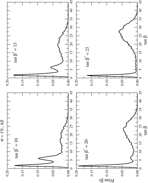
FIG. 1.: Histogram for the estimated $\tan\beta$ minimizing $\chi^{2}$. The experimental data included in the fit are all the observables discussed in the main text. We assume a precision $\sigma=1\%$ on all data. The energy range is $0.6<\sqrt{s}<1.0$ TeV in this and the following figures. The four boxes show what happens at the particular values 10, 15, 20 and 25 of the parameter $\tan\beta^{*}$ that, we recall, is the true value.

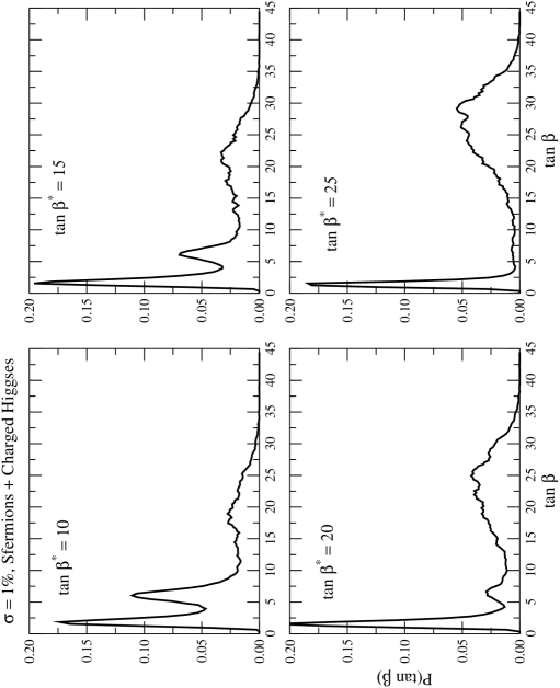
FIG. 2.: This figure is similar to Fig. (1), but $\chi^{2}$ minimization is performed by considering only the observables associated to the production of sfermions and charged Higgses.

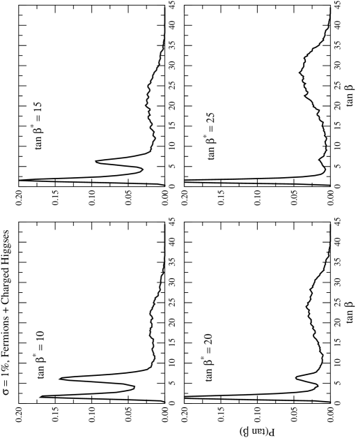
FIG. 3.: This figure is similar to Fig. (1), but $\chi^{2}$ minimization is performed by considering only the observables associated to the production of heavy fermions (top and bottom) and charged Higgses.

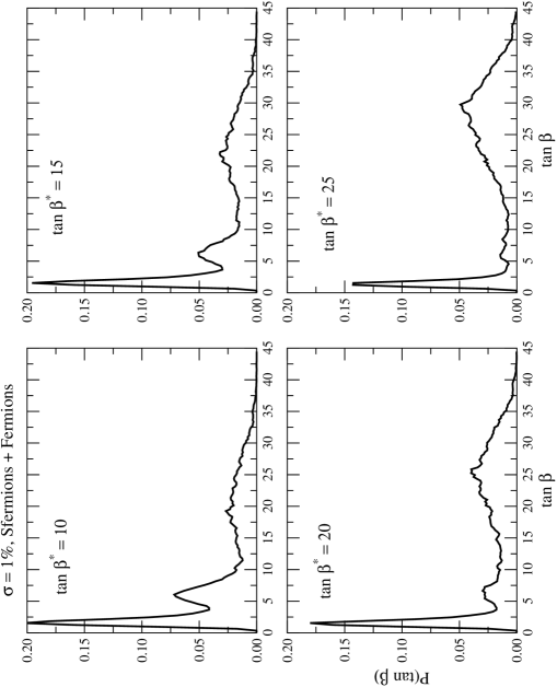
FIG. 4.: As a final case, this figure is again similar to Fig. (1), but $\chi^{2}$ minimization is performed by considering only the observables associated to the production of heavy fermions (top and bottom) and sfermions.

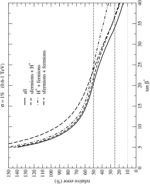
FIG. 5.: This figure shows the relative error in the estimate of $\tan\beta$ as a function of the true unknown value $\tan\beta^{*}$. The four curves correspond to the different set of observables considered in the previous figures, as described in the legend.

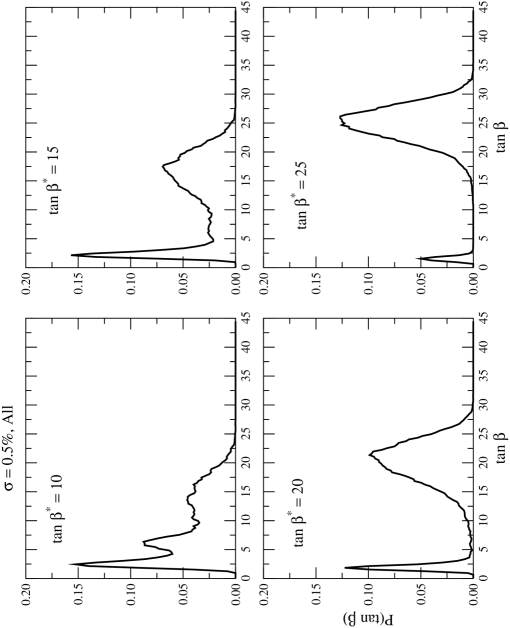
FIG. 6.: The analysis of the results shown in this figure is precisely the same as in Fig. (1), but with a global precision on the data reduced to $\sigma=0.5\%$.

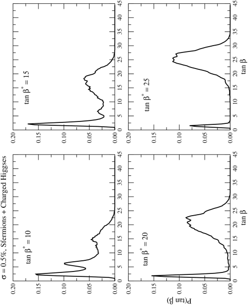
FIG. 7.: The analysis of the results shown in this figure is precisely the same as in Fig. (2), but with a global precision on the data reduced to $\sigma=0.5\%$.

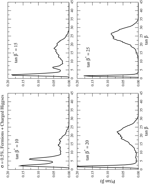
FIG. 8.: The analysis of the results shown in this figure is precisely the same as in Fig. (3), but with a global precision on the data reduced to $\sigma=0.5\%$.

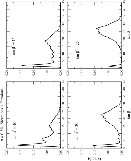
FIG. 9.: The analysis of the results shown in this figure is precisely the same as in Fig. (4), but with a global precision on the data reduced to $\sigma=0.5\%$.

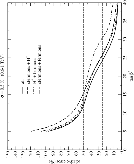
FIG. 10.: The analysis of the results shown in this figure is precisely the same as in Fig. (5), but with a global precision on the data reduced to $\sigma=0.5\%$.

REFERENCES

- [1] see e.g., E. Accomando et.al., Phys. Rep. C299, 299, (1998).
- [2] The CLIC study of a multi-TeV linear collider, CERN-PS-99-005-LP (1999).
- [3] M. Beccaria, F.M. Renard and C. Verzegnassi, Phys. Rev. D63, 095010 (2001).
- [4] M. Beccaria, S. Prelovsek, F. M. Renard and C. Verzegnassi, Phys. Rev. D64, 053016 (2001).
- [5] M. Beccaria, M. Melles, F. M. Renard and C. Verzegnassi, Phys.Rev.D65, 093007 (2002).
- [6] M. Beccaria, F. M. Renard and C. Verzegnassi, Phys.Rev.D63, 053013 (2001).
- [7] M. Beccaria, F. M. Renard, S. Trimarchi, and C. Verzegnassi, hep-ph/0212167.
- [8] see e.g. A. Datta, A. Djouadi and J.-L. Kneur, Phys. Lett. B509, 299 (2001); J. Gunion, T. Han, J. Jiang, A. Sopczak. hep-ph/0212151.