Some aspects of Dalitz decay $\pi^{0}\rightarrow e^{+}e^{-}\gamma$

Abstract

A calculation of $\pi^{0}\rightarrow e^{+}e^{-}\gamma$ in next-to-leading order in chiral perturbation theory of two flavour case extended by virtual photons is presented. The whole kinematic sector is covered and realistic experimental situation is discussed.

1 Introduction

With a branching ratio of $(1.198\pm 0.032)\%$ [1] the three body decay $\pi^{0}\rightarrow e^{+}e^{-}\gamma$, first considered by R. H. Dalitz more than fifty years ago [2], is the second most important decay channel of the pion. The dominant decay mode, $\pi^{0}\rightarrow\gamma\gamma$, with its overwhelming branching ratio of $\text{BR}=(98.798\pm 0.032)\%$, is deeply connected with this three body decay. The other decay channels connected with the anomalous $\pi^{0}\gamma\gamma$ vertex, like $\pi^{0}\rightarrow e^{+}e^{-}$ and $\pi^{0}\rightarrow 2(e^{+}e^{-})$, are suppressed approximately by respective factors of $10^{-7}$ and of $10^{-5}$. As already alluded to, the hadronic aspects of the Dalitz decay of the neutral pion are related to the axial anomaly. Actually, the main features of this process can be discussed within the framework of Chiral Perturbation Theory (ChPT – for reviews see [3]). In the case at hand, we need only to consider the case of two light quark flavours, $u$ and $d$. We shall however use the extension of ChPT to electromagnetic interaction, i.e. including effects of virtual photons [4], treating e.g. the pion mass difference as a $p^{2}$ effect at lowest order.

2 Kinematics

One may separate the contributions to the $\pi^{0}\rightarrow e^{+}e^{-}\gamma$ process into two main classes. The first corresponds to the Feynman graphs where the electron-positron pair is produced by a single photon (Dalitz pair). The leading contribution, of order $\alpha^{3}$, to the decay rate belongs to this one-photon reducible class, which involves a semi-off-shell $\pi^{0}\gamma\gamma$ vertex. The second class of contributions corresponds to one-photon irreducible topologies. They start with the radiative corrections to the $\pi^{0}\rightarrow e^{+}e^{-}$ process, which involves the doubly off-shell $\pi^{0}\gamma\gamma$ vertex. Their contributions to the decay rate are thus suppressed, being at least of order $\alpha^{5}$. For the time being, we shall therefore not take them into account. A complete discussion will appear elsewhere [5].

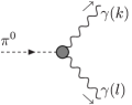
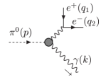
Figure 1: Kinematics lay for $\pi^{0}\rightarrow\gamma\gamma$ and $\pi^{0}\rightarrow e^{+}e^{-}\gamma$

The general expression of the one-photon reducible part of the $\pi^{0}(p)\rightarrow e^{+}(q_{1})e^{-}(q_{2})$ $\gamma(k)$ amplitude is of the form

$${\cal M}_{1\gamma R}(\pi^{0}\rightarrow e^{+}e^{-}\gamma)\,=\,{\cal M}_{\nu}g^{\nu\rho}\,\frac{(-i)}{(q_{1}+q_{2})^{2}}\,\frac{1}{1+{\overline{\Pi}}((q_{1}+q_{2})^{2})}\,\\ \times{\bar{u}}(q_{2})(ie)\Gamma_{\rho}(q_{2},q_{1})v(q_{1})\,.$$ (1)

In this expression, ${\cal M}_{\mu}(p,k)$ represents the semi-off-shell $\pi^{0}\gamma\gamma$ amplitude, defined as

$${\cal M}^{\mu}(p,k)\equiv\langle\gamma(k);{\rm out}|j^{\mu}(0)|\pi^{0}(p);{\rm in}\rangle={\cal A}((p-k)^{2})\varepsilon^{\nu\mu\alpha\beta}\epsilon_{\nu}(k)^{*}k^{\alpha}p^{\beta}\,,$$ (2)

where the second expression follows from Lorentz invariance and parity conservation, while $j^{\mu}$ denotes the electromagnetic current. Furthermore, ${\overline{\Pi}}\left((q_{1}+q_{2})^{2}\right)$ denotes the renormalized vacuum polarization function, with ${\overline{\Pi}}(0)=0$, and $\Gamma_{\rho}(q_{2},q_{1})$ stands for the vertex function, renormalized in the on-shell scheme, of the current $j_{\rho}$. Assuming again parity conservation, one may express $\Gamma_{\rho}(q_{2},q_{1})$ in terms of two form factors

$$\Gamma_{\rho}(q_{2},q_{1})=F_{1}\left((q_{1}+q_{2})^{2}\right)\gamma_{\rho}+F_{2}\left((q_{1}+q_{2})^{2}\right)\frac{i}{2m}\sigma_{\rho\sigma}(q_{1}+q_{2})^{\sigma}.$$ (3)

The Dirac form factor $F_{1}$ is thus normalized by $F_{1}(0)=1$, while the Pauli form factor gives the anomalous magnetic moment of the electron, $F_{2}(0)=a_{e}$. Finally, since $(q_{1}+q_{2})^{\mu}{\cal M}_{\mu}(p,k)=0$, the photon propagator reduces to the contribution of the $g^{\nu\rho}$ piece.

It is convenient to introduce the following kinematic parameters

$$x =\frac{(q_{1}+q_{2})^{2}}{m_{\pi^{0}}^{2}},\qquad \nu^{2} \leq x\leq 1,\qquad\nu^{2}=\frac{4m^{2}}{m_{\pi^{0}}^{2}}\,,$$ (4)

$$y =\frac{2p\cdot(q_{1}-q_{2})}{m_{\pi^{0}}^{2}(1-x)},\qquad -\beta \leq y\leq\beta,\qquad\beta=\sqrt{1-\frac{\nu^{2}}{x}}.$$ (5)

One may then write the partial decay rate, normalized to the $\pi^{0}\rightarrow\gamma\gamma$ decay rate $\Gamma_{0}=(1/64\pi){\cal A}(0)m_{\pi^{0}}^{3}$, for the one photon reducible contribution in terms of these parameters as

$$\frac{1}{\Gamma_{0}}\frac{d\Gamma}{{\rm d}x{\rm d}y} =\frac{\alpha}{\pi}\Bigl{|}\frac{{\cal A}(m_{\pi^{0}}^{2}x)}{{\cal A}(0)}\frac{1}{1+{\overline{\Pi}}(m_{\pi^{0}}^{2}x)}\Bigr{|}^{2}\frac{(1-x)^{3}}{4\,x^{2}}\Bigl{\{}\left|F_{1}(m_{\pi^{0}}^{2}x)\right|^{2}(\nu^{2}+xy^{2}+x)$$

$$+\left|F_{2}(m_{\pi^{0}}^{2}x)\right|^{2}\frac{x(\nu^{2}-xy^{2}+x)}{\nu^{2}}+4{\rm Re}(F_{1}(m_{\pi^{0}}^{2}x)F_{2}^{*}(m_{\pi^{0}}^{2}x))x\Bigr{\}},$$ (6)

or, by integrating out the parameter $y$

$$\frac{1}{\Gamma_{0}}\frac{d\Gamma}{{\rm d}x} =\frac{\alpha}{\pi}\Bigl{|}\frac{{\cal A}(m_{\pi^{0}}^{2}x)}{{\cal A}(0)}\frac{1}{1+{\overline{\Pi}}(m_{\pi^{0}}^{2}x)}\Bigr{|}^{2}\frac{(1-x)^{3}}{3\,x^{2}}\beta\Bigl{\{}\left|F_{1}(m_{\pi^{0}}^{2}x)\right|^{2}(\nu^{2}+2x)$$

$$+\left|F_{2}(m_{\pi^{0}}^{2}x)\right|^{2}\frac{x(2\nu^{2}+x)}{\nu^{2}}+6{\rm Re}(F_{1}(m_{\pi^{0}}^{2}x)F_{2}^{*}(m_{\pi^{0}}^{2}x))x\Bigr{\}}.$$ (7)

At lowest order in the fine structure constant we have ${\bar{\Pi}}=0$, $F_{1}=1$ and $F_{2}=0$. We shall discuss ${\cal A}$ and the hadronic part of ${\overline{\Pi}}$ in the next section.

3 Parameterization of Hadronic Part

We are going to study the problem in two flavour Chiral Perturbation Theory extended by virtual photons [3, 4, 6, 7] up to one loop, i.e. for this type of process up to the ${\cal O}(p^{6})$ where $p$ can represent momenta relevant for the decay or electromagnetic constant $e$. The lowest order effective Lagrangian can be written as

$${\cal L}^{(2)}=\frac{F^{2}}{4}\langle{\rm d}^{\mu}U^{+}{\rm d}_{\mu}U+\chi^{+}U+U^{+}\chi\rangle-\frac{1}{4}F^{\mu\nu}F_{\mu\nu}+ZF^{4}\langle Q_{R}UQ_{L}U^{+}\rangle$$ (8)

with

$$U={\rm e}^{\frac{i\phi}{F_{0}}},\quad\phi=\left(\begin{array}[]{cc}\pi^{0}&\sqrt{2}\pi^{+}\\ \sqrt{2}\pi^{-}&-\pi^{0}\end{array}\right).$$ (9)

Further chiral invariant Lagrangians of higher order (${\cal O}(p^{4})$ and ${\cal O}(p^{6})$), so-called Wess-Zumino anomaly Lagrangian (of ${\cal O}(p^{4})$ order) and also the other details of calculation within ChPT can be found in above references.

We will calculate the hadronic part of one photon reducible amplitude of the decay $\pi^{0}\rightarrow e^{+}e^{-}\gamma$, as it is depicted in Fig.2, i.e. the value of ${\cal A}(1-\bar{\Pi}_{had})$ in the terms of the previous section.

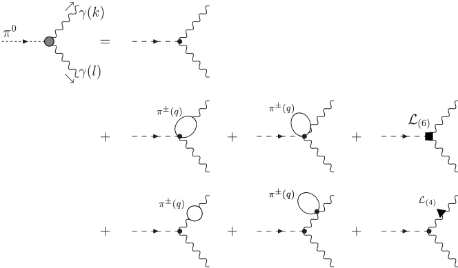
Figure 2: Leading order and pion loop contributions to the amplitude ${\cal M}_{1\gamma R}\propto{\cal A}(1-\bar{\Pi}_{had})$. To simplify the figure, we have omitted the $e^{+}e^{-}\gamma$-vertex. The graphs in the second row correspond to the corrections to ${\cal A}$, while the third row contributes by the factor $1-\bar{\Pi}_{had}$.

With definition $\sigma\equiv\sqrt{1-4m_{\pi^{\pm}}^{2}/{l^{2}}}$ one can obtain from the one photon irreducible graphs in Fig.2

$${\cal A}(l^{2})=-\frac{N_{C}e^{2}}{12\pi^{2}F_{\pi^{0}}}\Bigl{\{}1-\frac{l^{2}}{6F_{0}^{2}}\frac{1}{(4\pi)^{2}}\Bigl{[}\log\frac{m_{\pi^{\pm}}^{2}}{m_{\pi^{0}}^{2}}+\tfrac{1}{3}-2\sigma^{2}\\ -\sigma^{3}\log\frac{\sigma-1}{\sigma+1}-\overline{{\scriptstyle\Delta}a}\Bigr{]}+\delta a\Bigr{\}},$$ (10)

while the one particle reducible graphs contribute by the factor $(1-\bar{\Pi}_{had})$, where the hadronic contribution to renormalized vacuum polarization function is

$$\bar{\Pi}_{had}(l^{2})=\frac{e^{2}}{48\pi^{2}}\Bigl{[}\tfrac{2}{3}+2\sigma^{2}+\sigma^{3}\log\frac{\sigma-1}{\sigma+1}\Bigl{]}\Bigr{\}}.$$ (11)

Here we have used standard handling with infinities ($\lambda$) for ${\cal O}(p^{6})$ constants:

$${\scriptstyle\Delta}a ={\scriptstyle\Delta}a^{r}+{\scriptstyle\Delta}\alpha\lambda$$

$$\delta a =\delta a^{r}$$ (12)

with renormalized quantities to be finite and

$${\scriptstyle\Delta}a^{r}=\frac{{\scriptstyle\Delta}\alpha}{32\pi^{2}}\bigl{(}\overline{{\scriptstyle\Delta}a}+\log\frac{m_{\pi^{0}}^{2}}{\mu^{2}}\bigr{)},\qquad{\scriptstyle\Delta}\alpha=-\frac{1}{12\pi^{2}}.$$ (13)

The ${\cal O}(p^{6})$ constants used in this text could be connected with form of [8] and [9] respectively as

$${\scriptstyle\Delta}a =\frac{8}{3}F_{0}^{2}(A_{2}-4A_{3})=\frac{8}{3}F_{0}^{2}c_{13}$$ (14)

$$\delta a =\frac{32}{3}\pi^{2}\Bigl{[}(A_{2}-2A_{3}-4A_{4})m_{\pi^{0}}^{2}+\frac{20}{3}(A_{4}+2A_{6})2\bar{m}B\Bigr{]}=$$

$$=\frac{64}{3}\pi^{2}\Bigl{[}(c_{11}-4c_{3}-4c_{7})m_{\pi^{0}}^{2}+\frac{4}{3}(5c_{3}+c_{7}+2c_{8})2\bar{m}B\Bigr{]}.$$ (15)

The influence of virtual photon is covered in (10) in the neutral pion decay constant $F_{\pi^{0}}$ [4]. Unfortunately this constant is not known very accurately $F_{\pi^{0}}=92\pm 4$ [1] and so in practice the charged pion decay constant is used $F_{\pi}=92.4$

$$F_{\pi^{0}}=F_{\pi}\Bigl{(}1-\frac{m_{\pi^{\pm}}^{2}}{16\pi^{2}F_{0}^{2}}\log\frac{m_{\pi^{\pm}}^{2}}{m_{\pi^{0}}^{2}}-\frac{e^{2}}{64\pi^{2}}\bigl{[}(3+\tfrac{4}{9}Z)\bar{k}_{1}-\tfrac{40}{9}Z\bar{k}_{2}-3\bar{k}_{3}-4Z\bar{k}_{4}\bigr{]}\Bigr{)}.$$ (16)

To cover this section we will introduce a slope parameter $a$ which is a parameter of linear expansion of ${\cal A}(1-\bar{\Pi}_{had})$ in $x$:

$${\cal A}(1-\bar{\Pi}_{had})\sim(1+ax)$$ (17)

4 Calculation at $e^{3}(1+p^{2}+e^{2})$ order

Now, to the above hadronic contribution we have to add also the QED corrections, which are in our case up to one loop level: lepton part of vacuum polarization function, vertex, bremsstrahlung and 2-photon triangle and box corrections. In the first approximation we will neglect 2-photon loop diagrams (for a polemic whether this is justified see also [10]). For one-photon exchange the following interesting relation holds (c.f.[11])

$$\Gamma(\pi^{0}\rightarrow e^{+}e^{-}\gamma)=2\int_{0}^{1}\frac{dx}{x}\frac{1}{\pi}{\rm Im}\Pi(s)\Gamma_{0}(s).$$ (18)

with the lepton part of spectral function of the photon propagator $\Pi(s)$. With ${\cal O}(p^{6})$ constants set equal zero and therefore (from (10), (11) and (17)) $a=-0.0024$ we can obtain numerically

$$\frac{\Gamma(\pi^{0}\rightarrow e^{+}e^{-}\gamma)}{\Gamma(\pi^{0}\rightarrow\gamma\gamma)}=0.01185+0.00010=0.01196,$$ (19)

where the second number represents loop-correction contributions. Comparing this with PDG’s number $\Gamma^{exp}(\pi\rightarrow e^{+}e^{-}\gamma)/\Gamma(\pi\rightarrow\gamma\gamma)=(1.213\pm 0.033)\%$ one can immediately see that the total decay rate is not very suitable for probing the smooth effects of the higher orders (e.g. tuning ChPT constants).

Therefore we will turn our attention to the differential decay rate, which can be calculated in one-photon case using the relation (obtained from (18))

$$\frac{{\rm d}\Gamma^{\rm rad}}{{\rm d}x}=\frac{2}{x}\Pi_{a}(x)\Gamma_{0}(x)+\int_{(\sqrt{x}+m_{\gamma}^{IR}/m_{\pi^{0}})^{2}}^{1}\frac{{\rm d}E}{E}\Pi_{b}(E,x)\Gamma_{0}(E),$$ (20)

where we have divided the spectral function to the virtual and real part

$$\frac{1}{\pi}{\rm Im}\Pi^{(4)}(p)=\Pi_{a}(p^{2})+\Pi_{b}(p^{2}).$$ (21)

From the first plot in Fig.3 we see that while the radiative effects for the total decay rate is small, the situation in the differential decay rate is opposite.

Figure 3: Differential decay rate $\frac{1}{\Gamma_{0}}\frac{{\rm d}\Gamma^{(rad)}}{{\rm d}x}$ (from (20)) and the dependence of $\delta(x)$ on ${{\scriptstyle\Delta}E}$

However, this approach is useful for a situation when the detector is entirely blind to photons. In a more realistic situation, the experimental resolution is such that it is possible to detect photons if only above the (small) energy ${{\scriptstyle\Delta}E}$. For this case we define $\delta(x,y)$ and $\delta(x)$

$$\frac{1}{\Gamma_{0}}\frac{{\rm d}^{2}\Gamma^{\rm rad}}{{\rm d}x{\rm d}y}=\delta(x,y)\frac{1}{\Gamma_{0}}\frac{{\rm d}^{2}\Gamma}{{\rm d}x{\rm d}y},\qquad\frac{1}{\Gamma_{0}}\frac{{\rm d}\Gamma^{\rm rad}}{{\rm d}x}=\delta(x)\frac{1}{\Gamma_{0}}\frac{{\rm d}\Gamma}{{\rm d}x}.$$ (22)

In Fig.3 (the second plot) we depicted how the $\delta(x)$ changes with parameter ${{\scriptstyle\Delta}E}$.

Up to now we have systematically neglected the graphs which arise from the two-virtual-photons exchange. We have performed this calculation and we found interesting behaviour of contribution to $\delta(x)$, particularly when $x$ is close to 1. In this domain

$$\delta(x\sim 1,y)\approx 0.1,$$ (23)

i.e. it represents approximately 10% of leading order and from the previous we could conclude that it is a important contribution to differential decay rate, which cannot be neglected. However, it will be difficult to test this area experimentally. Actually for

$$x\gtrsim 1-\frac{2{{\scriptstyle\Delta}E}}{m_{\pi^{0}}}$$ (24)

the photon is effectively immeasurable by definition and precisely this is the domain where the interesting situation of (23) occurs. Let us also stress that in this part of calculation we have neglected the electron mass and thus, at this level, it is not possible to compare and use in our consideration process $\pi^{0}\rightarrow e^{+}e^{-}$ which is proportional to $m_{e}$ (for more details see [12]).

5 Conclusion

We have discussed the Dalitz decay $\pi^{0}\rightarrow e^{+}e^{-}\gamma$ in two flavour ChPT and set the hadronic part within this effective theory. Using PDG’s value for the slope parameter (see (17)) $a=0.032\pm 0.004$ [1] one can estimate following linear combination of ${\cal O}(p^{6})$ constants

$$\frac{m_{\pi^{0}}^{2}}{6F_{0}^{2}}\frac{1}{(4\pi)^{2}}\overline{{\scriptstyle\Delta}a}-a\delta a=a+0.0024$$

(cf. (13) and (14)). We approve that the effects of higher orders in total decay rate are smaller than the present experimental error (19). However, differential decay rate is much sensitive to these effects.
Acknowledgement.  This work was supported in part by the program “Research Centres” project number LN00A006 of the Ministry of Education of the Czech Republic, Socrates/Erasmus programme and EC contract HPRN-CT-2002-00311 (EURIDICE).

References

- [1] K. Hagiwara et al. Phys. Rev. D 66 (2002) 010001.
- [2] R.H. Dalitz, Proc.Phys.Soc.(London) A64 (1951) 667.
- [3] J. Gasser and H. Leutwyler, Annals Phys. 158 (1984) 142; J. Gasser and H. Leutwyler, Nucl. Phys. B 250 (1985) 465, 517, 539; H. Leutwyler, Annals Phys. 235 (1994) 165 [arXiv:hep-ph/9311274].
- [4] R. Urech, Nucl. Phys. B 433 (1995) 234 [arXiv:hep-ph/9405341]; M. Knecht and R. Urech, Nucl. Phys. B 519 (1998) 329 [arXiv:hep-ph/9709348].
- [5] K. Kampf, M. Knecht, J. Novotný: in preparation.
- [6] R. Kaiser, Phys. Rev. D 63 (2001) 076010 [arXiv:hep-ph/0011377].
- [7] K. Kampf and J. Novotny, Acta Phys. Slov. 52 (2002) 265 [arXiv:hep-ph/0210074].
- [8] H. W. Fearing and S. Scherer, Phys. Rev. D 53 (1996) 315 [arXiv:hep-ph/9408346].
- [9] J. Bijnens, L. Girlanda and P. Talavera, Eur. Phys. J. C 23 (2002) 539 [arXiv:hep-ph/0110400].
- [10] G. B. Tupper, T. R. Grose and M. A. Samuel, Phys. Rev. D 28 (1983) 2905; M. Lambin and J. Pestieau, Phys. Rev. D 31 (1985) 211; L. Roberts and J. Smith, Phys. Rev. D 33 (1986) 3457; G. Tupper, Phys. Rev. D 35 (1987) 1726.
- [11] B. E. Lautrup and J. Smith, Phys. Rev. D 3 (1971) 1122.
- [12] M. Knecht, S. Peris, M. Perrottet and E. de Rafael, Phys. Rev. Lett. 83 (1999) 5230 [arXiv:hep-ph/9908283].