The radiative return at $\mathbf{\phi}$- and B-factories: small-angle photon emission at next to leading order

Abstract

The radiative return offers the unique possibility for a measurement of the cross section of electron–positron annihilation into hadrons over a wide range of energies. The large luminosity of present $\phi$- and B-factories easily compensates for the additional factor of $\alpha$ due to the emission of a hard photon. Final states with photons at large angles can be easily identified. The rate for events with collinear photons, however, is enhanced by a large logarithm and allows, in particular at lower energies, for a complementary measurement. The Monte Carlo generator PHOKHARA, which includes next to leading order corrections from virtual and real photon emission, has been extended from large photon angles into the collinear region, using recent results for the virtual corrections. In addition, the present version includes final state radiation for muon and pion pair production and final states with four pions. Implications for the experimental analysis at three typical energies, 1.02, 4 and 10.6 GeV, are presented: the magnitude of these new corrections is studied, possibilities for the separation of initial and final state radiation are proposed, and the differences with respect to the previous treatment based on structure functions are investigated.

1 Introduction

Measurements of the cross section for electron–positron annihilation into hadrons are essential for the interpretation of the recent, precise results for the muon anomalous magnetic moment $a_{\mu}$ Brown:2001mg . Similarly they are relevant for our knowledge of the running of the fine structure constant and thus crucial for the analysis of electroweak precision measurements at high energy colliders Jegetc. ; HMNT02 ; Davier:2002dy .

Of particular importance for these two applications is the low energy region, say from threshold up to centre-of-mass system (cms) energies of approximately 3 GeV for $a_{\mu}$ and 10 GeV for $\alpha(M_{Z})$. Recent measurements based on energy scans between 2 and 5 GeV have improved the accuracy in part of this range BES . Similar, or even further improvements below 2 GeV would be highly welcome. The region between 1.4 GeV and 2 GeV, in particular, is poorly studied and no collider will cover this region in the near future. Improvements on the precise measurements of the pion form factor in the low energy region by the CMD2 and DM2 collaborations CMD2 , or even an independent cross-check, would be extremely useful, in particular in view of the disagreement between $e^{+}e^{-}$data and the analysis based on isospin-breaking-corrected $\tau$ decays Davier:2002dy .

Traditionally the energy dependence of the cross section was deduced from experiments, where the beam energy was varied over the range dictated by the energy reach of the collider. This ‘energy scan’ allows, at a first glance, a fairly simple interpretation of the measurement in terms of the so called R-ratio, which enters the aforementioned applications. Nevertheless also in this case initial state radiative corrections (ISR) give rise to complications and require a complicated unfolding procedure discussed below.

As an alternative the ‘radiative return’ has been suggested Binner:1999bt ; Melnikov:2000gs ; Czyz:2000wh ; Spagnolo:1999mt as a particularly attractive option for $\phi$- and B-meson factories. These collider experiments operate at fixed energies, albeit with enormous luminosities. BABAR and BELLE at 10.6 GeV, CLEO-C in the region between 3 and 5 GeV and KLOE at 1.02 GeV are the experiments of interest for the subsequent considerations. This peculiar feature of a ‘factory’ allows the use of the radiative return, i.e. the reaction

$$e^{+}(p_{1})+e^{-}(p_{2})\to\gamma(k_{1})+\gamma^{*}(Q)\left(\to{\rm hadrons}\right)\ \ ,$$ (1)

to explore a wide range of $Q^{2}$ in a single experiment.

Nominally invariant masses of the hadronic system between the production threshold of the respective channel and the cms energy of the experiment are accessible. In practice, to clearly identify the reaction, it is useful to consider only events with a hard photon–tagged or untagged–which lowers the energy significantly.

To arrive at reliable predictions for differential and for partially integrated cross sections, including kinematical cuts as used in experiments, a Monte Carlo generator is indispensable. The inclusion of radiative corrections in the generator and in the experimental analysis is essential for the precise extraction of the cross section. For hadronic states with invariant masses below 2 to 3 GeV, it is desirable to simulate the individual channels with two, three and up to six mesons, i.e. pions, kaons, $\eta$’s, etc., which requires a fairly detailed parametrisation of various form factors.

A first program called EVA was constructed some time ago Binner:1999bt to simulate the production of a pion pair together with a hard photon. It includes initial state radiation, final state radiation (FSR), their interference, and the dominant radiative corrections from additional collinear radiation through structure function (SF) technique CCR . A similar program that simulates the production of four pions together with a hard photon has been developed in Czyz:2000wh . More recently a new Monte Carlo generator called PHOKHARA RCKS was developed. It includes, in contrast to the former generators, the complete next-to-leading order (NLO) radiative corrections.

The first version of PHOKHARA incorporates ISR only and is limited to $\pi^{+}\pi^{-}\gamma(\gamma)$ and $\mu^{+}\mu^{-}\gamma(\gamma)$ as final states. PHOKHARA exhibits, however, a modular structure that simplifies the implementation of additional ha-dronic modes or the replacement of the current(s) of the existing modes. Its first version was designed to simulate configurations with photons emitted at relatively large angles, $\theta^{2}\gg m_{e}^{2}/s$. In this case it is legitimate to drop terms proportional to $m^{2}_{e}$, an assumption that leads to a considerable simplification of the virtual corrections Rodrigo:2001jr . Subsequently analytical results for the virtual corrections, that are also valid into the small angle region, were obtained in RK02 . The extension of the program PHOKHARA into this small angle region, incorporating these new analytic results are the central topic of the present paper. The description of this new feature and numerous tests of the program stability and technical precision are contained in Section 2.

Final state radiation can affect the measurement of the pion form factor, and quite generally of the R-ratio. However, using suitable cuts, its effects can be significantly reduced. Moreover, given sufficiently large event rates its magnitude can be extracted experimentally by varying the cuts and/or comparing events with different photon angles with respect to beam and pion directions, respectively. The charge asymmetry that arises from ISR–FSR interference provides another important handle on this ‘background’. For this reason FSR from $\pi^{+}\pi^{-}$ and $\mu^{+}\mu^{-}$ has been incorporated in the upgrade of the program and will be discussed in Section 3. The $\mu^{+}\mu^{-}$ final state is still limited to its QED part, e.g. the narrow resonances (J/$\psi$) are not (yet) included.

The program has also been extended to include final states with four pions, following the lines discussed in Czyz:2000wh . The implementation of these new channels will be discussed in Section 4.

2 The radiative return for small-angle emission and tests of the program

The study of events with photons emitted under both large and small angles, and thus at a significantly enhanced rate, is particularly attractive for the $\pi^{+}\pi^{-}$ final state with its clear signature Aloisio:2001xq ; Denig:2001ra ; Adinolfi:2000fv ; Barbara:Morion ; Venanzoni:2002 ; Achim:radcor02 . In contrast events with a tagged photon, emitted at a large angle, have a clear signature particularly suited to the analysis of hadronic states of higher multiplicities babar ; Berger:2002mg .

The inclusion of radiative corrections is essential for the precise extraction of the cross section, which is necessarily based on a Monte Carlo simulation. The complete NLO corrections have recently been implemented in the program PHOKHARA. However, just like the earlier EVA, this program was designed for photon emission at large angles (‘tagged photons’). For nearly collinear photons, corrections from virtual and real photon emission, as well as Born terms, must include those contributions proportional to $m_{e}^{2}/s$ and even to $m_{e}^{4}/s^{2}$, which are enhanced by their highly singular angular dependence and thus integrate to terms of order 1 and proportional to $\alpha/\pi$ for Born and NLO terms respectively. These mass-suppressed terms are significantly smaller than the leading, logarithmically enhanced pieces; they must nevertheless be taken into account for a consistent treatment. The evaluation of corrections from virtual plus soft photon emission to reaction (1), valid for the full angular region, has been treated in RK02 . Essentially it consists of the calculation of the leptonic tensor $L_{\mu\nu}$, which has to be multiplied by the hadronic tensor $H_{\mu\nu}$, so that a fully differential distribution is obtained. To arrive at a reasonably compact, numerically stable result, the limit $m_{e}^{2}/s\ll 1$ for $L_{\mu\nu}$ is considered. However, terms proportional to $m_{e}^{2}$ must be kept if these exhibit the singular angular dependence discussed above.

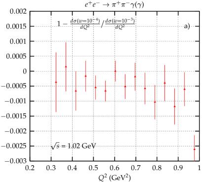
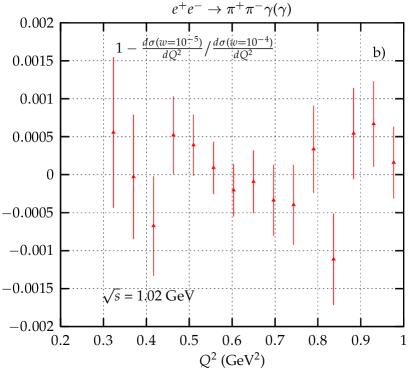
Figure 1: Comparison of the $Q^{2}$ differential distribution for different values of the soft photon cutoff: $w=10^{-3}$ vs. $10^{-4}$ and $w=10^{-4}$ vs. $10^{-5}$ , at $\sqrt{s}=1.02$ GeV. One of the photons was required to have energy $>$ 10 MeV. No further cuts were applied.

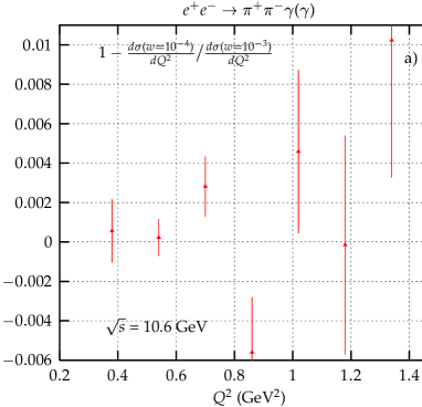
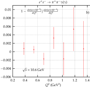
Figure 2: Comparison of the $Q^{2}$ differential distribution for different values of the soft photon cutoff: $w=10^{-3}$ vs. $10^{-4}$ and $w=10^{-4}$ vs. $10^{-5}$ , at $\sqrt{s}=10.6$ GeV. One of the photons was required to have energy $>$ 100 MeV. No further cuts were applied.

The differential rate for the virtual and soft QED corrections is thus cast into the product of a leptonic and a hadronic tensor and the corresponding factorised phase space:

$$d\sigma = \frac{1}{2s}L_{\mu\nu}d\Phi_{2}(p_{1}+p_{2};Q,k_{1})$$ (2)

$$\times H^{\mu\nu}d\Phi_{n}(Q;q_{1},\cdots,q_{n})\frac{dQ^{2}}{2\pi}\ \ ,$$

where $d\Phi_{n}(Q;q_{1},\cdots,q_{n})$ denotes the hadronic $n$-body phase space, including all statistical factors, $Q^{2}$ is the invariant mass of the hadronic system and $d\Phi_{2}(p_{1}+p_{2};Q,k_{1})$ is the two-body phase space of the photon and the hadronic system. The tensor $L_{\mu\nu}$ depends on the four-vectors $p_{1}$, $p_{2}$, $Q$, $k_{1}$ and the soft photon cutoff $w\equiv E_{\gamma}^{\mathrm{max}}/\sqrt{s}$. Its explicit functional form is given in RK02 . The description of the hadronic system is model-dependent. It enters only through the hadronic tensor

$$H^{\mu\nu}=J^{\mu}J^{\nu\dagger}\ ,$$ (3)

where the hadronic current has to be parametrised through form factors Czyz:2000wh ; Kuhn:1990ad ; Decker:1994af ; Ecker:2002cw . The running of $\alpha$ is not taken into account in this program and can be included trivially in the final experimental analysis.

Table 1: Total cross section (nb) for the process $e^{+}e^{-}\rightarrow\pi^{+}\pi^{-}\gamma$ at NLO for different values of the soft photon cutoff. Only initial state radiation. One of the photons with energy larger than 10 MeV for $\sqrt{s}=1.02$ GeV and larger than 100 MeV for $\sqrt{s}=10.6$ GeV. $Q^{2}<1$GeV. No further cuts applied.

$w$	$\sqrt{s}=$1.02 GeV	10.6 GeV
$10^{-3}$	36.999 (3)	0.15557(7)
$10^{-4}$	37.021 (3)	0.15548(6)
$10^{-5}$	37.021 (3)	0.15545(6)

The matrix element for the emission from the initial state of two real hard photons, i.e. $E_{\gamma_{i}}>w\sqrt{s}$, with $i=1,2,$

$$e^{+}(p_{1})+e^{-}(p_{2})\to\gamma^{*}(Q)+\gamma(k_{1})+\gamma(k_{2})\ \ ,$$ (4)

is calculated numerically following the helicity amplitude method with the conventions introduced in Kolodziej:1991pk ; Jegerlehner:2000wu . The results from RCKS , which were used for tagged photon events are equally applicable for the present purpose.

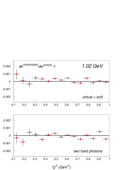
Figure 3: Comparison of the virtual+soft and hard contributions to the $\pi^{+}\pi^{-}$ differential cross section with inclusive analytical results. Soft photon cutoff: $w=10^{-4}$.

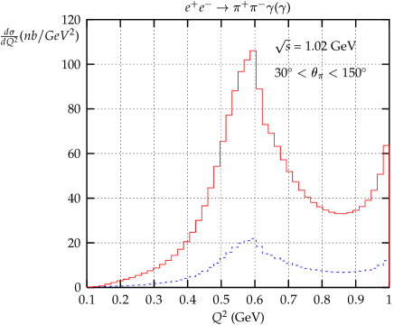
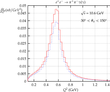
Figure 4: Comparison of the $Q^{2}$ differential cross sections for $\sqrt{s}=$ 1.02 (left) and 10.6 GeV (right). The pion angles are restricted to $30^{\circ}<\theta_{\pi^{\pm}}<150^{\circ}$, while the photon(s) angles are not restricted (upper curves) and restricted to $30^{\circ}<\theta_{\gamma}<150^{\circ}$ (lower curves).

The virtual plus soft photon contribution and the hard one depend separately on the soft photon cutoff $w$ used to regulate the infrared divergences of the virtual diagrams. The former shows a logarithmic $w$-dependence. The latter, after numerical integration of the phase space, exhibits the same behaviour, whereas their sum must be independent of $w$. To show that this indeed occurs is therefore a basic test of the performance of the program. The value of $w$ that optimises the efficiency of the event generation, avoiding at the same time the appearance of the negative weights, is determined by this procedure.

Table 1 presents the total cross section for radiative production of a pair of pions calculated for several values of the soft photon cutoff at two different cms energies. The energy of one of the photons was required to be larger than 10 MeV for $\sqrt{s}=1.02$ GeV and larger than 100 MeV for $\sqrt{s}=10.6$ GeV. No further kinematical cuts were applied, thus allowing to test in particular the small photon angle region.

For $\sqrt{s}=1.02$ GeV the comparison between $w=10^{-3}$ and $10^{-4}$ indicates a residual $w$-dependence. The excellent agreement between $w=10^{-4}$ and $10^{-5}$, within the error of the numerical integration, confirms the $w$-independence of the result. A value around $w=10^{-4}$ seems to be the best choice as observed before for large angle photons RCKS ; Rodrigo:2002hk .

In Figs. 1 and 2 the $Q^{2}$ dependence of the differential cross section $d\sigma/dQ^{2}$ is compared for different choices of the cutoff, after integration over the remaining kinematic variables. Again for $\sqrt{s}=1.02$ GeV the comparison between $w=10^{-3}$ and $10^{-4}$ shows a residual $w$ dependence (Fig. 1a), which disappears beyond $w=10^{-4}$ (Fig. 1b). At a cms energy of 10.6 GeV the result is numerically stable for $w=10^{-3}$ already (Fig. 2a). Stable results are also obtained for $w$ around and below $10^{-4}$ (Fig. 2b). Thus $w=10^{-4}$ is used as the default value in the program. Similar tests were performed for the four-pion channels (see Section 4).

The present implementation of PHOKHARA covers the full angular region for photon emission. This allows for a number of tests and comparisons with analytical results that were not possible with the previous version. In Fig. 3 the results of the program are compared with the analytical results from Ref. Berends:1988ab . We use their Eqs. (2.25)+(2.26) for the virtual plus soft part and Eq. (2.28) for the hard emission part. As it was necessary to change several couplings in the original formulae, we repeat (Appendix B) the expressions actually used for the comparison. Agreement within the statistical uncertainty and in any case better than $10^{-3}$ is evident from this comparison.

Initial state radiation is dominated by photons at small angles. Inclusion of events with nearly collinear photons thus leads to a significant enhancement of the observed event rate. The comparison between the differential cross sections for large angle photon events $(30^{\circ}<\theta_{\gamma}<150^{\circ})$ and without restriction on $\theta_{\gamma}$ is shown in Fig. 4. The pion angles are always assumed to be restricted to the region $30^{\circ}<\theta_{\pi^{\pm}}<150^{\circ}$. Results are presented for two different cms energies ( $\sqrt{s}=$ 1.02 and 10.6 GeV). There is a big quantitative difference between these two energies. For $\sqrt{s}$ = 1.02 GeV a huge contribution from small angle photons is observed for the full range of $Q^{2}$. In contrast the gain in the cross section for $\sqrt{s}=$ 10.6 GeV is small as a consequence of the conflicting kinematical constraints of small photon and large pion angles. FSR has not been included in these figures. For 10.6 GeV its contribution is negligible, while for 1.02 GeV and for the cuts used for Fig. 4 it is sizeable, but can be reduced using the cuts discussed below.

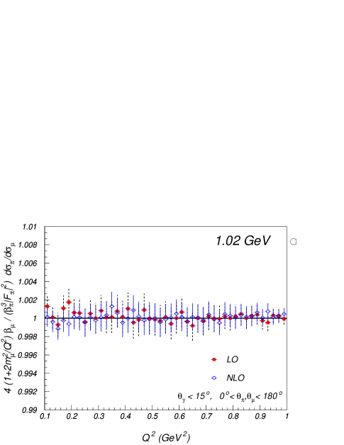
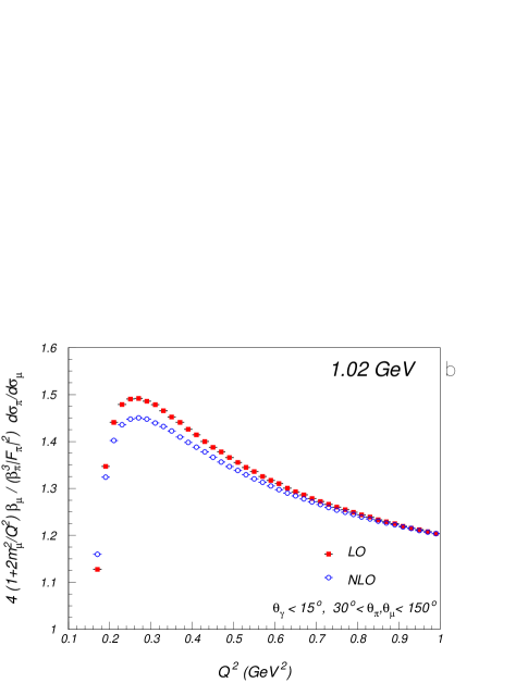
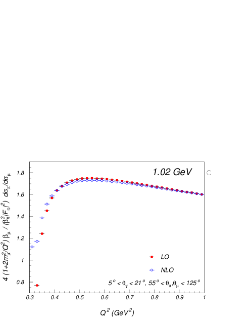
Figure 5: Ratio between pion and muon yields, after dividing through their respective R-ratio. a: no cuts on pion and muon angles; b: with angular cuts on pion and muon angles; c: with angular cuts on pion and muon angles and ‘large’ angle photons.

The R-ratio can in principle be deduced either from the measurement of the hadronic cross section, which requires a precise control of the luminosity, or from the ratio between hadronic and $\mu^{+}\mu^{-}$ event rates. Various radiative corrections, e.g. from the running of the electromagnetic coupling and from ISR cancel in the ratio between the hadronic and $\mu^{+}\mu^{-}$ rates. Indeed, one obtains by construction unity, if one considers the properly normalised ratio

$$\rho_{\pi\mu}\equiv\frac{4(1+2m_{\mu}^{2}/Q^{2})\beta_{\mu}}{\beta_{\pi}^{3}\mid F_{\pi}\mid^{2}}\ \ \frac{d\sigma_{\pi^{+}\pi^{-}\gamma(\gamma)}}{d\sigma_{\mu^{+}\mu^{-}\gamma(\gamma)}}\ \ ,$$ (5)

where

$$\beta_{i}=\sqrt{1-\frac{4m_{i}^{2}}{Q^{2}}}\ ,\ \ i=\pi,\mu\ \ ,$$

and $F_{\pi}$ is the pion form factor.

The result $\rho_{\pi\mu}=1$ is independent of the restrictions on the photon angular region and is true in Born and NLO approximations. The phase space of hadronic and $\mu^{+}\mu^{-}$ final states, however, must be fully integrated (Fig. 5a). For realistic cuts on pion and muon angles the ratio deviates significantly from 1, a consequence of their markedly different angular distributions. The size of this effect depends on the details of the cuts on photon, pion and muon angles as demonstrated in Figs. 5b and 5c. In both figures, one observes a significant, few per cent, difference between Born and NLO predictions for $\rho_{\pi\mu}$, depending on the details of the cuts on the photon and charged particle angles. At 10.6 GeV the ratio $\rho_{\pi\mu}$ is of course again equal to 1 if pions and muons are fully integrated (Fig. 6a). In contrast to the situation at lower energies, the inclusion of realistic cuts does not alter this picture drastically, a consequence of the high correlation between photon and pion or muon angles: photon and charged particles are essentially emitted back to back (Fig. 6b).

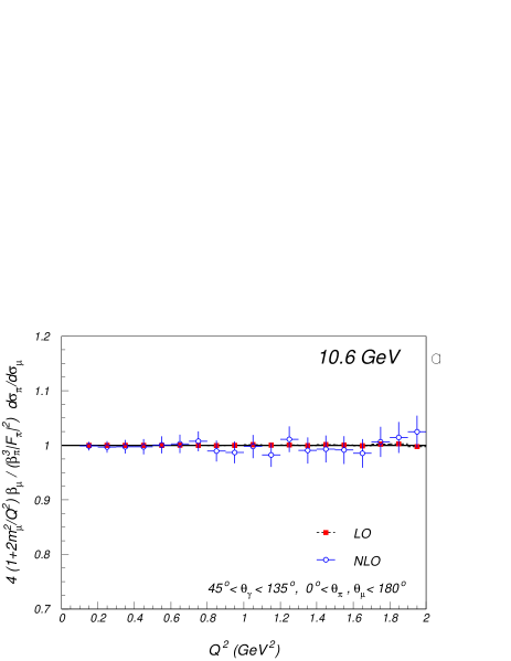
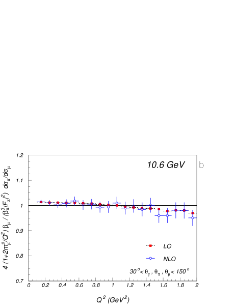
Figure 6: Ratio between pion and muon yields, after dividing through their respective R-ratio. a: no cuts on pion and muon angles; b: with angular cuts on pion and muon angles.

The shape of these curves depends only on the pion and muon angular distributions, but not on the form factor itself. These results can thus be directly used to deduce efficiencies of specific experimental cuts in a model-independent way, since pion and muon angular distributions are fixed by general considerations. For more complicated final states (e.g. $4\pi$, $KK\pi$, $\cdots$) the corresponding ratio would, instead of $|F_{\pi}|^{2}\beta_{\pi}^{3}/4$, directly involve the corresponding R-ratio, if no cuts on the hadrons are applied. Otherwise the results depend on the model for the hadronic form factor implemented in the program. An important advantage of the radiative return is implicit in all these considerations: by measuring $Q^{2}$ directly, the invariant squared mass of the hadronic final state, one has direct access to R at the corresponding value of $Q^{2}$. This differs from the measurement of the inclusive cross section as a function of $\sqrt{s}$ (energy scan). To extract the true R($s$), an unfolding has to be performed, which requires in principle the knowledge of the cross section over the full energy range below and a precise knowledge of the radiator function. In contrast, using the radiative return method, it is still necessary to know the QED radiator function, but no unfolding is required as one measures the $Q^{2}$ of the hadronic system, and thus has ‘access’ to the hadronic cross section at that given $Q^{2}$.

Let us discuss those $\alpha m_{e}^{2}/s$ and $\alpha(m_{e}^{2}/s)^{2}$ terms, which in combination with their singular angular dependence integrate to corrections of order $\alpha/\pi$. These are included in the present version of PHOKHARA. The corresponding leading order corrections proportional to $m_{e}^{2}$ are typically of the order of a few per cent Rodrigo:2001cc , while the non-leading ones are of order 0.1%. This can be seen from Fig. 7. The size of these effects is consistent with the expectations for $\alpha/\pi$ terms without logarithmic enhancement. These terms will become important when the precision of the measurement will be below 1%. Their proper treatment is in that case crucial as they do depend on $Q^{2}$ and do change the $Q^{2}$ distribution from which the hadronic cross section is extracted.

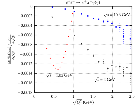
Figure 7: The relative contributions of the non-leading mass corrections to the differential cross section at $\sqrt{s}$ = 1, 4 and 10 GeV.

3 Initial versus final state radiation

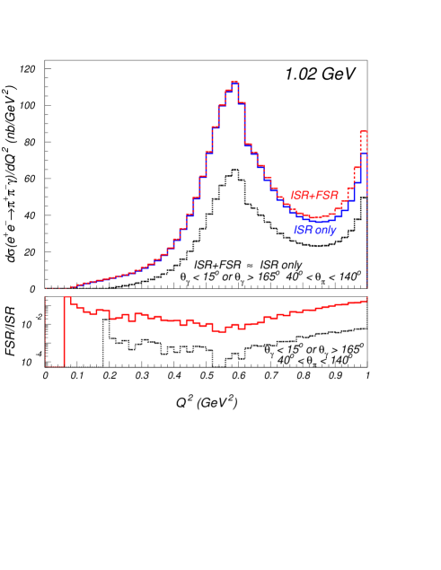
Figure 8: The suppression of the FSR contributions to the cross section by a suitable choice of angular cuts. Results from the PHOKHARA generator. No cuts (upper curves) and suitable cuts applied (lower curves).

A potential complication for the measurement of the pion form factor or generally of the R-ratio may arise from the interplay between photons from ISR and FSR. Their relative strength is strongly dependent on the photon angle relative to the beam and the pion directions, the cms energy of the reaction and the invariant mass of the hadronic system. FSR from hadronic final states cannot be predicted from first principles and thus has to be modelled. The model amplitude can nevertheless be tested by considering charge-asymmetric differential distributions, which arise from the interference between ISR and FSR amplitudes Binner:1999bt . In leading order the complete matrix element squared is given by

$$|{\cal M}|^{2}=|{\cal M}_{\mathrm{ISR}}|^{2}+|{\cal M}_{\mathrm{FSR}}|^{2}+2\mathrm{Re}[{\cal M}_{\mathrm{ISR}}{\cal M}_{\mathrm{FSR}}^{\dagger}]~{},$$ (6)

which is still independent of the model for FSR.

FSR and its interference with ISR were already included in EVA Binner:1999bt for the two-pion case. The pions were assumed to be point-like, and scalar QED was applied to simulate photon emission off the charged pions. It was demonstrated there that ISR dominates for suitably chosen final states, namely those with hard photons at small angles relative to the beam, well separated from the pions. FSR can therefore be reduced to a reasonable limit, and moreover, can be controlled by the simulation (see also CDKMV2000 ). Similar results can be obtained using the new version of PHOKHARA, were FSR and ISR–FSR interference are included for two pions and muons (see Appendix A for details) at LO. The photon emission from pions is again modelled by a point–like pion-photon interaction. The upper two curves of Fig. 8 describe the differential cross section with arbitrary photon and pion angles. The contribution of FSR is clearly visible. Once photon emission is restricted to angles close to the beam and if the pion- and photon-allowed angular ranges do not overlap (lower curve), FSR is clearly negligible.

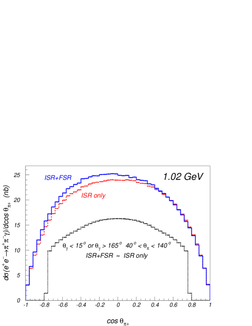
Figure 9: Angular distribution of $\pi^{+}$ with and without FSR for different angular cuts.

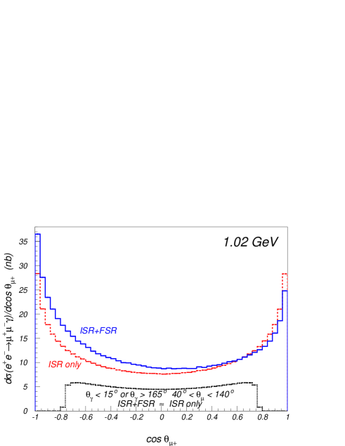
Figure 10: Angular distribution of $\mu^{+}$ with and without FSR for different angular cuts.

The third term in the right-hand side of Eq. (6), ISR–FSR interference, is odd under charge conjugation, and its contribution vanishes after angular integration. It gives rise, however, to a relatively large charge asymmetry and, correspondingly, to a forward–backward asymmetry

$$A(\theta)=\frac{N^{\pi^{+}}(\theta)-N^{\pi^{+}}(\pi-\theta)}{N^{\pi^{+}}(\theta)+N^{\pi^{+}}(\pi-\theta)}~{}.$$ (7)

The asymmetry can be used for calibration of the FSR amplitude, and fits to the angular distribution $A(\theta)$ can test details of its model dependence. Given sufficiently large event rates this procedure can be performed for different $\theta_{\gamma}$, thus allowing for an unambiguous reconstruction of the FSR amplitude.

This is illustrated in Figs. 9 and 10, where the angular distributions of $\pi^{+}$ and $\mu^{+}$ respectively are shown for different kinematical cuts. The angles are defined with respect to the incoming positron. If no angular cut is applied, the angular distribution in both cases is highly asymmetric as a consequence of the ISR–FSR interference contribution. If cuts suitable to suppress FSR, and therefore the ISR–FSR interference, are applied, the distributions become symmetric.

These investigations can also be performed for different photon energies, thus exploring FSR in different regions of $Q^{2}$. We will return to this aspect in a future publication.

Figure 11: Angular distribution of $\pi^{+}$ at $\sqrt{s}$=10.6 GeV (ISR $\simeq$ FSR+ISR).

At B-factories, where one has to deal with very hard tagged photons, the kinematic separation between the photon and the hadrons becomes very clear. For events where hadrons and photon are produced mainly back to back, the suppression of FSR is naturally accomplished and no special angular cuts are therefore needed to control FSR versus ISR at higher energies (Fig. 11). The relative size of the FSR is of the order of a few per mil, but does depend on the value of the pion form factor at $\sqrt{s}$ = 10 GeV, which is extrapolated from the low energy data.

The suppression of FSR contributions to $\pi^{+}\pi^{-}\gamma$ events is also a consequence of the rapid decrease of the form factor above $\sim$ 1 GeV. It is therefore instructive to study the corresponding distributions for $\mu^{+}\mu^{-}\gamma$ final states. For $\sqrt{Q^{2}}\leq$ 1 GeV FSR is still tiny. Around 3 GeV a small charge-asymmetric interference term becomes visible (Fig. 12), which is still irrelevant after averaging over $\mu^{+}$ and $\mu^{-}$. At large $Q^{2}$, however, FSR plays an important role both for the charge-asymmetry and the charge symmetric term.

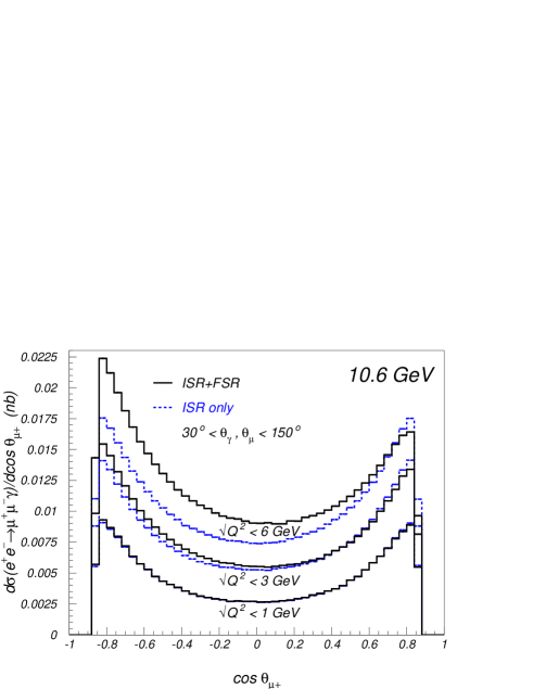
Figure 12: Angular distribution of $\mu^{+}$ at $\sqrt{s}$=10.6 GeV for various $Q^{2}$ cuts.

4 The four-pion mode

Figure 13: Diagrams contributing to the 4$\pi$ hadronic current.

Because of the modular structure of PHOKHARA, additional hadronic modes can be easily implemented. The four-pion channels ($2\pi^{+}2\pi^{-}$ and $2\pi^{0}\pi^{+}\pi^{-}$), which give the dominant contribution to the hadronic cross section in the region from 1 to 2 GeV, are a new feature of our event generator.

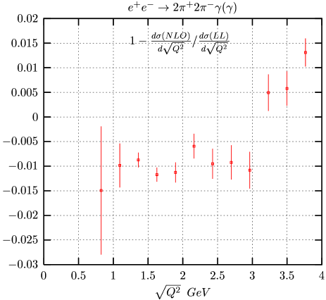
Figure 14: The relative non-leading contributions to the differential cross section at $\sqrt{s}$ = 4 GeV. NLO - full next-to-leading result, LL - leading logarithmic approximation.

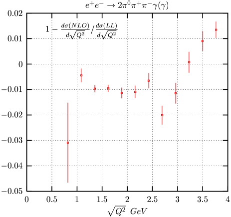
Figure 15: The relative non-leading contributions to the differential cross section at $\sqrt{s}$ = 4 GeV. NLO - full next-to-leading result, LL - leading logarithmic approximation.

Isospin invariance relates the amplitudes of the $e^{+}e^{-}\to 2\pi^{+}2\pi^{-}$ and $e^{+}e^{-}\to 2\pi^{0}\pi^{+}\pi^{-}$ processes and those for $\tau$ decays into $\pi^{-}3\pi^{0}$ and $\pi^{+}2\pi^{-}\pi^{0}$ K2 ; Czyz:2000wh . The description of the four-pion hadronic current follows Czyz:2000wh ; Decker:1994af . The basic building blocks of this current are schematically depicted in Fig. 13 and described in detail in Czyz:2000wh .

Results obtained with PHOKHARA for these channels have been compared with the Monte Carlo, which simulates the same process at LO Czyz:2000wh and includes additional collinear radiation through the SF technique. Typically, differences of order 1$\%$ are found (see Figs. 14 and  15), which are of the expected size and of the same order as for the two-pion final state RCKS .

The generation of the pion four momenta is however different from the one described in Czyz:2000wh . In the present version of the program we absorb the most prominent peaks in the four-pion hadronic current to obtain a more efficient Monte Carlo generation. The $Q^{2}$ distribution is peaked around $\sqrt{Q^{2}}$ = 1.5 GeV, with a large width of $\sim$ 0.5 GeV. This is the result of an interplay between several resonances present in that region. Nevertheless one Breit–Wigner resonance provides an adequate approximation for efficient generation. For the approximant and the generation of the $Q^{2}$ distribution we use

$$f_{3}(Q^{2})=\frac{s}{s-Q^{2}}+\frac{s^{2}}{(Q^{2}-m^{2})^{2}+\Gamma^{2}m^{2}}\ ,$$ (8)

with $m=1.5$ GeV and $\Gamma=$ 0.5 GeV.

It takes care of soft photon emission ($s-Q^{2}\sim E_{\gamma}$ ) and the aforementioned resonant behaviour. For the process $e^{+}e^{-}\to 2\pi^{0}\pi^{+}\pi^{-}\gamma(\gamma)$ we furthermore absorb the $\omega$ peaks in the four momentum squared $Q_{0+-}^{2}=p_{\omega}^{2}=(p_{0}+p_{+}+p_{-})^{2}$. The approximant used for that purpose, according to which the three-particle four momenta squared are generated, reads

$$f_{4}(Q_{134}^{2},Q_{234}^{2})=2$$

$$+\frac{m_{\omega}\Gamma_{\omega}}{(Q_{134}^{2}-m_{\omega}^{2})^{2}+\Gamma_{\omega}^{2}m_{\omega}^{2}}+\frac{m_{\omega}\Gamma_{\omega}}{(Q_{234}^{2}-m_{\omega}^{2})^{2}+\Gamma_{\omega}^{2}m_{\omega}^{2}}\ ,$$ (9)

where $Q_{134}$ and $Q_{234}$ are the four momenta of the two $\pi^{0}\pi^{+}\pi^{-}$ subsystems. The other variables are generated as described in Czyz:2000wh .

Table 2: Total cross section (nb) for the process $e^{+}e^{-}\rightarrow 4\pi\gamma$ at NLO for different values of the soft photon cutoff at $\sqrt{s}=$ 1.02 GeV. Only initial state radiation. One of the photons with energy $>$ 10 MeV. $Q^{2}<1$GeV. No further cuts applied.

$w$	$2\pi^{+}2\pi^{-}$	$2\pi^{0}\pi^{+}\pi^{-}$
$10^{-3}$	0.170167(15)	0.55725(5)
$10^{-4}$	0.170413(14)	0.55844(5)
$10^{-5}$	0.170431(15)	0.55845(5)

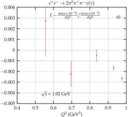
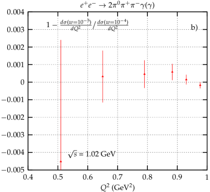
Figure 16: The relative difference of the differential cross sections for two different values of the soft photon cutoff at $\sqrt{s}$ = 1.02 GeV. One of the photons was required to have energy $>$ 10 MeV. No further cuts were applied.

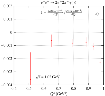
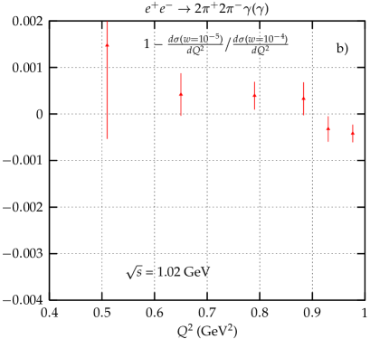
Figure 17: The relative difference of the differential cross sections for two different values of the soft photon cutoff at $\sqrt{s}$ = 1.02 GeV. One of the photons was required to have energy $>$ 10 MeV. No further cuts were applied.

Also for the four-pion modes, we have tested the independence of the result of the soft–hard separation parameter $w$. The results are very much similar to the $\pi^{+}\pi^{-}$ mode and are summarised in Table 2 and Figs. 16 and 17. Again the choice $w=10^{-4}$ is the proper one.

5 Conclusions

The Monte Carlo generator PHOKHARA, which simulates the radiative return at electron–positron colliders, has been extended from large angles into the collinear region using recent results for the virtual corrections to photon emission, which are valid for all photon angles. Comparing the program with analytical results, a technical precision better than $0.5\times 10^{-3}$ is demonstrated. The importance of NLO corrections for the extraction of a correct value for the R-ratio is emphasised.

A number of corrections vanish if the ratio between hadron and muon pair cross section is considered. For low energies, around 1 GeV, the ratio depends strongly on the cuts on the charged particles and corrections have to be applied. At higher energies, around 10 GeV, and for low $Q^{2}$, the dependence on these cuts is drastically reduced.

In the new version of PHOKHARA, described in this article, final state radiation in leading order treatment is included. We discuss the implications for the measurement of the pion form factor. Suitable cuts allow, on the one hand, the determination of this model-dependent amplitude, on the other hand it is possible to select configurations that are entirely dominated by initial state radiation.

Finally we extend the program final states with four-pions configuration as a first step towards the inclusion of a multitude of exclusive states.

Appendix A The implementation of the final state emission

Final state emission of one photon and the final-initial state interference terms are implemented in the present program in lowest order by means of the helicity amplitude method for both $\pi^{+}\pi^{-}\gamma$ and $\mu^{+}\mu^{-}\gamma$ final states. The notation is the same as in RCKS and will not be repeated. The pion-photon interaction is adopted from scalar electrodynamics.

The helicity amplitudes describing the initial emission read

$$M_{\mathrm{ISR}}(\lambda_{e^{+}},\lambda_{e^{-}},\lambda_{1})=\frac{(4\pi\alpha)}{Q^{2}}\biggl{\{}$$

$$v_{I}^{\dagger}(p_{1},\lambda_{e^{+}})A\ u_{I}(p_{2},\lambda_{e^{-}})+v_{II}^{\dagger}(p_{1},\lambda_{e^{+}})B\ u_{II}(p_{2},\lambda_{e^{-}})\biggl{\}}\ ,$$ (10)

where

$$A =\frac{\left(\varepsilon^{*}(k_{1},\lambda_{1})^{-}k_{1}^{+}-2\varepsilon^{*}(k_{1},\lambda_{1})\cdot p_{1}\right)J^{-}}{2k_{1}\cdot p_{1}}$$

$$+\frac{J^{-}\left(2\varepsilon^{*}(k_{1},\lambda_{1})\cdot p_{2}-k_{1}^{+}\varepsilon^{*}(k_{1},\lambda_{1})^{-}\right)}{2k_{1}\cdot p_{2}}$$ (11)

and

$$B =\frac{\left(\varepsilon^{*}(k_{1},\lambda_{1})^{+}k_{1}^{-}-2\varepsilon^{*}(k_{1},\lambda_{1})\cdot p_{1}\right)J^{+}}{2k_{1}\cdot p_{1}}$$

$$+\frac{J^{+}\left(2\varepsilon^{*}(k_{1},\lambda_{1})\cdot p_{2}-k_{1}^{-}\varepsilon^{*}(k_{1},\lambda_{1})^{+}\right)}{2k_{1}\cdot p_{2}}\ .$$ (12)

The current $J^{\mu}$ for $\pi^{+}\pi^{-}$ in the final state reads

$$J^{\mu}_{2\pi}=ieF_{2\pi}(Q^{2})\;(q_{\pi^{+}}-q_{\pi^{-}})^{\mu}~{},$$ (13)

while for $\mu^{+}\mu^{-}$ in the final state it is given by

$$J^{\mu}_{2\mu}(\lambda_{\mu^{+}},\lambda_{\mu^{-}})=ie\bar{u}(q_{1},\lambda_{\mu^{-}})\gamma^{\mu}v(q_{2},\lambda_{\mu^{+}})\ \ .$$ (14)

The part of the amplitude that comes from the final state emission can be written as

$$M_{\mathrm{FSR}}(\lambda_{e^{+}},\lambda_{e^{-}},\lambda_{1})=\frac{(4\pi\alpha)}{s}\biggl{\{}$$

$$v_{I}^{\dagger}(p_{1},\lambda_{e^{+}})D^{-}u_{I}(p_{2},\lambda_{e^{-}})+v_{II}^{\dagger}(p_{1},\lambda_{e^{+}})D^{+}u_{II}(p_{2},\lambda_{e^{-}})\biggl{\}}\ ,$$ (15)

where the four-vector $D^{\mu}$ reads

$$D^{\mu}(\lambda_{1})=ieF_{2\pi}(s)\biggl{\{}\left(q_{1}+k_{1}-q_{2}\right)^{\mu}\frac{q_{1}\cdot\varepsilon^{*}(k_{1},\lambda_{1})}{q_{1}\cdot k_{1}}$$

$$+\left(q_{2}+k_{1}-q_{1}\right)^{\mu}\frac{q_{2}\cdot\varepsilon^{*}(k_{1},\lambda_{1})}{q_{2}\cdot k_{1}}-2\varepsilon^{*\mu}(k_{1},\lambda_{1})\biggr{\}}\ ,$$ (16)

for $\pi^{+}\pi^{-}$ in the final state, while for $\mu^{+}\mu^{-}$ in the final state it is

$$D^{\mu}(\lambda_{1},\lambda_{\mu^{+}},\lambda_{\mu^{-}})=ie\biggl{\{}$$

$$u_{I}^{\dagger}(q_{2},\lambda_{\mu^{-}})\tilde{A}^{\mu}v_{I}(q_{1},\lambda_{\mu^{+}})+u_{II}^{\dagger}(q_{2},\lambda_{\mu^{-}})\tilde{B}^{\mu}v_{II}(q_{1},\lambda_{\mu^{+}})\biggl{\}}\ ,$$ (17)

with

$$\tilde{A}^{\mu} =\frac{\left(\varepsilon^{*}(k_{1},\lambda_{1})^{-}k_{1}^{+}+2\varepsilon^{*}(k_{1},\lambda_{1})\cdot q_{2}\right)\sigma^{\mu-}}{2k_{1}\cdot q_{2}}$$

$$-\frac{\sigma^{\mu-}\left(2\varepsilon^{*}(k_{1},\lambda_{1})\cdot q_{1}+k_{1}^{+}\varepsilon^{*}(k_{1},\lambda_{1})^{-}\right)}{2k_{1}\cdot q_{1}}\ ,$$ (18)

and

$$\tilde{B}^{\mu} =\frac{\left(\varepsilon^{*}(k_{1},\lambda_{1})^{+}k_{1}^{-}+2\varepsilon^{*}(k_{1},\lambda_{1})\cdot q_{2}\right)\sigma^{\mu+}}{2k_{1}\cdot q_{2}}$$

$$-\frac{\sigma^{\mu+}\left(2\varepsilon^{*}(k_{1},\lambda_{1})\cdot q_{1}+k_{1}^{-}\varepsilon^{*}(k_{1},\lambda_{1})^{+}\right)}{2k_{1}\cdot q_{1}}\ .$$ (19)

The FSR matrix element squared and the FSR–ISR interference for pions in the final state agrees numerically (15 digits) with the code of EVA Binner:1999bt , if non-leading mass terms $\sim m_{e}^{2}$ missing in EVA are added. The largest relative change of the matrix element squared due to those missing terms is however as small as $10^{-6}$. The sum over polarisations of the squared matrix element for muon final states is numerically identical to the result obtained by means of the trace method using FORM FORM . For both final states the external gauge invariance was checked numerically, while one can see at a glance that the above analytical formulae have that property.

To analyse the contribution from FSR the program can be run in three different options: initial state radiation only, initial state radiation plus final state radiation without interference and complete result with interference terms. In the last two cases it is necessary to change the generation of the phase space to absorb final state emission peaks. For these two options we use three channels to absorb the peaks in $Q^{2}$ and in pion (muon) angular distributions. For the muon case we use the approximant

$$f_{1}(q^{2},\cos(\theta_{\mu}))=\frac{1}{1-q^{2}}+\frac{1}{q^{2}}$$

$$+\frac{1}{1-q^{2}}\left(\frac{1}{1-v(m_{\mu})\cos(\theta_{\mu})}+\frac{1}{1+v(m_{\mu})\cos(\theta_{\mu})}\right)\ ,$$ (20)

where

$$v(m)=\sqrt{1-\frac{4m^{2}}{s}}\ \ ,\ \ q^{2}=\frac{Q^{2}}{s}\ \ ,$$ (21)

For the pion case we use

$$f_{2}(q^{2},\cos(\theta_{\pi}))=\frac{1}{1-q^{2}}+\frac{1}{(q^{2}-m_{\rho}^{2}/s)^{2}+\Gamma_{\rho}^{2}m_{\rho}^{2}/s^{2}}$$

$$+\frac{1}{1-q^{2}}\left(\frac{1}{1-v(m_{\pi})\cos(\theta_{\pi})}+\frac{1}{1+v(m_{\pi})\cos(\theta_{\pi})}\right)\ .$$ (22)

An appropriate change of variables allows for a smoothing of the aforementioned peaks. The $q^{2}$ and $\cos(\theta_{\mu(\pi)})$ are generated according to the functions $f_{1(2)}(q^{2},\cos(\theta_{\mu(\pi)}))$. These very simple approximants work well enough to allow for relatively fast event generation.

Appendix B The analytical formulae used in Section 2

The formulae resulting from the analytical evaluation of the integration over photon angles are adopted from Refs. Berends:1986yy ; Berends:1988ab (see also Section 2 for details). The contributions of the virtual + soft corrections to the hadronic invariant mass ($Q^{2}$) differential distribution are given by

$$Q^{2}\frac{d\sigma}{dQ^{2}}=\frac{4\alpha^{3}}{3s}R(Q^{2})\bigg{\{}\frac{1+q^{4}}{1-q^{2}}(L-1)$$

$$\times\bigg{(}1+\frac{\alpha}{\pi}\;\bigg{[}\log(4w^{2})(L-1)+\frac{3}{2}L-2+\frac{\pi^{2}}{3}\bigg{]}\bigg{)}$$

$$+\frac{\alpha}{\pi}\;\bigg{[}-\frac{1+q^{4}}{2(1-q^{2})}\;\log(q^{2})\;L^{2}$$

$$+\bigg{\{}\frac{1+q^{4}}{1-q^{2}}\bigg{(}\hbox{Li}_{2}(1-q^{2})+\log(q^{2})\log(1-q^{2})$$

$$\quad-\frac{\log^{2}(q^{2})}{2}+\frac{5}{2}\log(q^{2})\bigg{)}-(1-q^{2})\log(q^{2})+\frac{q^{2}}{2}\bigg{\}}L$$

$$+\frac{1+q^{4}}{1-q^{2}}\bigg{(}S_{1,2}(1-q^{2})+\bigg{[}\log(q^{2})-\frac{3}{2}\bigg{]}\hbox{Li}_{2}(1-q^{2})$$

$$\quad+\bigg{[}\log(q^{2})\log(1-q^{2})-\frac{\log^{2}(q^{2})}{3}+\log(q^{2})$$

$$\quad-3\log(1-q^{2})-8\bigg{]}\frac{\log(q^{2})}{2}\bigg{)}$$

$$+(1+q^{2})\bigg{(}2\hbox{Li}_{3}(1-q^{2})-S_{1,2}(1-q^{2})$$

$$\quad-\log(1-q^{2})\hbox{Li}_{2}(1-q^{2})+\frac{\log^{2}(q^{2})}{4}\bigg{)}$$

$$+\frac{1-7q^{2}}{2}\bigg{(}\hbox{Li}_{2}(1-q^{2})+\log(q^{2})\log(1-q^{2})\bigg{)}$$

$$-\frac{1-5q^{2}}{4}\bigg{(}\log^{2}(1-q^{2})+\frac{2\pi^{2}}{3}\bigg{)}$$

$$+\frac{3-2q^{2}}{2}\log(1-q^{2})+\frac{7-5q^{2}}{2}\log(q^{2})-1\bigg{]}\bigg{\}}~{},$$ (23)

While the emission of two hard photons, i.e. both photons with energy larger than $w\sqrt{s}$, contributes as

$$Q^{2}\frac{d\sigma}{dQ^{2}}=\frac{4\alpha^{3}}{3s}R(Q^{2})\frac{\alpha}{\pi}$$

$$\times\bigg{[}\frac{1+q^{4}}{1-q^{2}}\bigg{\{}2\log(\frac{1-q^{2}}{2w})-\frac{\log(q^{2})}{2}\bigg{\}}(L-1)^{2}$$

$$+\bigg{\{}-(1-q^{2})+(1+q^{2})\frac{\log(q^{2})}{2}\bigg{\}}L^{2}$$

$$+\bigg{\{}\frac{7}{2}(1-q^{2})-q^{2}\log(q^{2})+(1+q^{2})\frac{\log^{2}(q^{2})}{4}\bigg{\}}L$$

$$+\frac{1+q^{4}}{1-q^{2}}\bigg{(}-S_{1,2}(1-q^{2})-\frac{\log(q^{2})}{2}\hbox{Li}_{2}(1-q^{2})$$

$$-\frac{3\log^{2}(q^{2})}{2}+\big{(}\frac{\pi^{2}}{6}+\frac{5}{3}\big{)}\log(q^{2})\bigg{)}$$

$$-(1+q^{2})\bigg{(}\frac{\hbox{Li}_{3}(1-q^{2})}{2}+S_{1,2}(1-q^{2})\bigg{)}-\frac{\pi^{2}q^{2}}{9}$$

$$-\bigg{(}\frac{1}{2}+\frac{2q^{2}}{3}\bigg{)}\hbox{Li}_{2}(1-q^{2})-(10-25q^{2})\frac{\log(q^{2})}{6}$$

$$+\bigg{(}\frac{2}{(1-q^{2})^{2}}-\frac{1}{4}-\frac{7q^{2}}{3}\bigg{)}\log^{2}(q^{2})$$

$$+\frac{1-q^{2}}{2}-\frac{2}{3}\frac{q^{2}}{1-q^{2}}\bigg{(}1+\frac{\log(q^{2})}{1-q^{2}}\bigg{)}^{2}\bigg{]}~{},$$ (24)

with $L=\log(s/m_{e}^{2})$ and $S_{1,2}$ the Nielsen’s generalised polylogarithm function

$$S_{n,p}(z)=\frac{(-1)^{n+p-1}}{(n-1)!\ p!}\int_{0}^{1}\log^{n-1}(t)\frac{\log^{p}(1-zt)}{t}dt~{},$$ (25)

$\hbox{Li}_{n}(z)=S_{n-1,1}(z)$ being the polylogarithms

$$\hbox{Li}_{n}(z)=\sum_{k=1}^{\infty}\frac{z^{k}}{k^{n}}~{},\qquad|z|<1~{},$$ (26)

and

$$S_{1,2}(1-z) =\frac{1}{2}\log^{2}(z)\log(1-z)+\zeta(3)$$

$$+\log(z)\hbox{Li}_{2}(z)-\hbox{Li}_{3}(z)~{}.$$ (27)

The function $R(Q^{2})$ is related to the hadronic current $J^{em}$ through

$${\kern-60.0pt}\int\ J^{em}_{\mu}(J^{em}_{\nu})^{*}\ \ d\bar{\Phi}_{n}(Q;q_{1},\dots,q_{n})=$$

$${\kern 20.0pt}\frac{1}{6\pi}\left(Q_{\mu}Q_{\nu}-g_{\mu\nu}Q^{2}\right)\ R(Q^{2})\ \ ,$$ (28)

where $d\bar{\Phi}_{n}(Q;q_{1},\dots,q_{n})$ denotes the $n$-body phase space with all statistical factors coming from the hadronic final state included.

The ratio $R(Q^{2})=$ $\sigma(e^{+}e^{-}\rightarrow{\mathrm{hadrons}})/\sigma_{point}$ for hadrons = $\pi^{+}\pi^{-}$ is equal to

$$R(Q^{2})=|F(Q^{2})|^{2}\frac{\beta_{\pi}^{3}}{4}\ .$$ (29)

References

- (1) H. N. Brown et al. [Muon Collaboration], Phys. Rev. Lett. 86 (2001) 2227 [hep-ex/0102017]; G.W.Bennett et al. [Muon Collaboration], Phys. Rev. Lett. 89 (2002) 101804, Erratum, ibid. 89 (2002) 129903, [hep-ex/0208001].
- (2) F. Jegerlehner, hep-ph/0104304.
- (3) K. Hagiwara, A.D. Martin, Daisuke Nomura and T. Teubner, hep-ph/0209187.
- (4) M. Davier, S. Eidelman, A. Höcker and Z. Zhang, hep-ph/0208177.
- (5) W.B. Yan, W.G. Li and Z.G. Zhao [BES Collaboration], hep-ex/021000.
- (6) R.R. Akhmetshin et al., Phys. Lett. B 527 (2002) 161 [hep-ex/0112031].
- (7) S. Binner, J. H. Kühn and K. Melnikov, Phys. Lett. B 459 (1999) 279 [hep-ph/9902399].
- (8) K. Melnikov, F. Nguyen, B. Valeriani and G. Venanzoni, Phys. Lett. B477 (2000) 114 [hep-ph/0001064].
- (9) H. Czyż and J. H. Kühn, Eur. Phys. J. C 18 (2001) 497 [hep-ph/0008262].
- (10) S. Spagnolo, Eur. Phys. J. C 6 (1999) 637.
- (11) M. Caffo, H. Czyż and E. Remiddi, Nuovo Cim. 110A (1997) 515 [hep-ph/9704443]; Phys. Lett. B 327(1994)369.
- (12) G. Rodrigo, H. Czyż, J.H. Kühn and M. Szopa, Eur. Phys. J. C 24 (2002) 71 [hep-ph/0112184].
- (13) G. Rodrigo, A. Gehrmann-De Ridder, M. Guilleaume and J. H. Kühn, Eur. Phys. J. C 22 (2001) 81 [hep-ph/0106132].
- (14) G. Rodrigo and J.H. Kühn, Eur. Phys. J. C 25 (2002) 215 [hep-ph/0204283].
- (15) A. Aloisio et al. [KLOE Collaboration], hep-ex/0107023.
- (16) A. Denig et al. [KLOE Collaboration], eConf C010430 (2001) T07 [hep-ex/0106100].
- (17) M. Adinolfi et al. [KLOE Collaboration], hep-ex/0006036.
- (18) B. Valeriani et al. [KLOE Collaboration], hep-ex/0205046.
- (19) G. Venanzoni et al. [KLOE Collaboration], hep-ex/0210013; hep-ex/0211005.
- (20) A. Denig et al. [KLOE Collaboration], hep-ex/0211024.
- (21) E. P. Solodov [BABAR collaboration], eConf C010430 (2001) T03 [hep-ex/0107027].
- (22) N. Berger, hep-ex/0209062.
- (23) J. H. Kühn and A. Santamaria, Z. Phys. C 48 (1990) 445.
- (24) R. Decker, M. Finkemeier, P. Heiliger and H. H. Jonsson, Z. Phys. C 70 (1996) 247 [hep-ph/9410260].
- (25) G. Ecker and R. Unterdorfer, Eur. Phys. J. C 24 (2002) 535 [hep-ph/0203075].
- (26) K. Kołodziej and M. Zrałek, Phys. Rev. D 43 (1991) 3619.
- (27) F. Jegerlehner and K. Kołodziej, Eur. Phys. J. C 12 (2000) 77 [hep-ph/9907229].
- (28) G. Rodrigo, H. Czyż and J. H. Kühn, hep-ph/0205097; hep-ph/0210287; hep-ph/0211186.
- (29) F. A. Berends, G. J. Burgers and W. L. van Neerven, Phys. Lett. B 177 (1986) 191.
- (30) F. A. Berends, W. L. van Neerven and G. J. Burgers, Nucl. Phys. B 297 (1988) 429; Erratum, ibid. B 304 (1988) 921.
- (31) G. Rodrigo, Acta Phys. Polon. B 32 (2001) 3833 [hep-ph/0111151].
- (32) G. Cataldi, A. Denig, W. Kluge, S. Muller and G. Venanzoni, Frascati Physics Series (2000) 569.
- (33) J.H. Kühn, Nucl. Phys. B (Proc. Suppl.) 76 (1999) 21.
- (34) J. A. M. Vermaseren, Symbolic Manipulations with FORM, Computer Algebra Nederland, Amsterdam, 1991.