Preface

N. Mankoč Borštnik e-mail:norma.s.mankocs@ijs.siInstitute of Nuclear Physics, N.C.S.R. Demokritos, 15310, Athens, GreeceInstitut für Theoretische Physik, Universität Heidelberg, Philosophenweg 16, D-69120, Heidelberg, GermanyDepartment of Physics and Astronomy Glasgow University, Glasgow G12 8QQ, ScotlandDepartment of Mathematical Sciences University of Durham, Durham DH1 3LE^(a) Department of Physics and Astronomy, University of North Carolina, Chapel Hill, NC 27599-3255. ^(b) Department of Physics, Boston University,Boston, MA 02215. ^(c) Department of Physics and Astronomy, Vanderbilt University,
Nashville, TN 37235.NIKHEF, Amsterdam NLThe Niels Bohr Institute, Copenhagen, DenmarkInstitute of Theoretical and Experimental Physics, Moscow, Russia The Niels Bohr Institute, Blegdamsvej 17 DK-2100 Copenhagen, DenmarkDepartment of Physics Stanford University, Stanford, CA 94305-4060ITEP, 117218 Moscow, Russia Physics and Astronomy Department, San Francisco State University, San Francisco, CA 94117 USA

One of the most important things in one person’s life is to have good friends, whom one can exchange thoughts and ideas with. The present volume is a collection of contributions by friends of Holger Bech Nielsen for his 60 th birthday. The collection of papers covers a broad range of physics, which shows that Holger Bech Nielsen has been working and is working on many topics — also because different fields of physics are much more connected as one would believe, at least when fundamental questions of physics are concerned. The most fascinating works in physics bring new understanding of known phenomena, since they lead to theories beyond the known ones. Holger Bech Nielsen is one of (very rare and because of that additionally precious ) scientists who is always willing to play with new thoughts and progressive ideas, trying to formulate them into formal proofs built on well defined assumptions and into formulas, pointing out in such a way that mathematics is a part of Nature.

It is my pleasure and my privilege to have Holger as a real friend in the last five years, since we have started — together with Colin Froggatt — the annual workshop at Bled, Slovenia, which is entitled “What comes Beyond the Standard Model”. During the workshop the ideas connected with the open problems of (elementary particle) physics and cosmology are very vividly and openly discussed.

The first volume of this Proceedings is a Festschrift dedicated to Holger. I wish to thank all his friends who are contributing to this volume and also to those friends, who have sent their contributions too late to be included.

The second volume is collecting contributions and discussions from the last two workshops and will appear with a little delay.

The editors would like to thank Yasutaka Takanishi for a lot of work, which contributed to make the Volume 1 of the Proceedings see the light of day.

Dear Holger: I am honoured to congratulate you for your 60th jubilee in the name of all your friends contributing to this volume and also in the name of the others, wishing you many additional fruitful years, health, wealth and success.

In the name of your friends:
Norma Susana Mankoč Borštnik           Ljubljana, December 2001

Workshops organized at Bled

$\triangleright$

What Comes beyond the Standard Model (June 29–July 9, 1998)

$\triangleright$

Hadrons as Solitons (July 6-17, 1999)

$\triangleright$

What Comes beyond the Standard Model (July 22–31, 1999)

$\triangleright$

Few-Quark Problems (July 8-15, 2000)

$\triangleright$

What Comes beyond the Standard Model (July 17–31, 2000)

$\triangleright$

Statistical Mechanics of Complex Systems (August 27–September 2, 2000)

$\triangleright$

What Comes beyond the Standard Model (July 17–27, 2001)

$\triangleright$

Studies of Elementary Steps of Radical Reactions in Atmospheric Chemistry (August 25–28, 2001)

Unified Internal Space of Spins and Charges

N. Mankoč Borštnik e-mail:norma.s.mankocs@ijs.siInstitute of Nuclear Physics, N.C.S.R. Demokritos, 15310, Athens, GreeceInstitut für Theoretische Physik, Universität Heidelberg, Philosophenweg 16, D-69120, Heidelberg, GermanyDepartment of Physics and Astronomy Glasgow University, Glasgow G12 8QQ, ScotlandDepartment of Mathematical Sciences University of Durham, Durham DH1 3LE^(a) Department of Physics and Astronomy, University of North Carolina, Chapel Hill, NC 27599-3255. ^(b) Department of Physics, Boston University,Boston, MA 02215. ^(c) Department of Physics and Astronomy, Vanderbilt University,
Nashville, TN 37235.NIKHEF, Amsterdam NLThe Niels Bohr Institute, Copenhagen, DenmarkInstitute of Theoretical and Experimental Physics, Moscow, Russia The Niels Bohr Institute, Blegdamsvej 17 DK-2100 Copenhagen, DenmarkDepartment of Physics Stanford University, Stanford, CA 94305-4060ITEP, 117218 Moscow, Russia Physics and Astronomy Department, San Francisco State University, San Francisco, CA 94117 USA

Abstract

Can the assumption that the spin and all the charges of either fermions or bosons unify, help to find the answers to the open questions of the electroweak Standard model? The approach is presented in which polynomials in Grassmann space are used to describe all the internal degrees of freedom of spinors, scalars and vectors, that is their spins and charges mankoc1992 ; mankoc1999 . The same can be achieved mankocandnielsen1999 also by polynomials of differential forms. If the space - ordinary and anti-commutative - has 14 dimensions or more, the appropriate spontaneous breaking of symmetry leads gravity in $d$ dimensions to manifest in four-dimensional subspace as ordinary gravity and all the gauge fields as well as the Yukawa couplings. The approach manifests four generations of massless fermions, which are left handed $SU(2)$ doublets and right handed $SU(2)$ singlets.

Abstract

Semitopological Vortices (Q-Rings) are identified to be classical soliton configurations whose stability is attributed to both topological and nontopological charges. We discuss some recent work on the simplest possible realization of such a configuration in a scalar field theory with an unbroken $U(1)$ global symmetry. We show that Q-Rings correspond to local minima of the energy, exhibit numerical solutions of their field configurations and derive virial theorems demonstrating their stability.

Abstract

We demonstrate that the amplitude $\langle\rho\gamma|\partial^{\nu}(\bar{q}\gamma_{\nu}\gamma_{5}q)|0\rangle$ does not vanish in the limit of zero quark masses. This represents a new kind of violation of the classical equation of motion for the axial current and should be interpreted as the axial anomaly for bound states. The anomaly emerges in spite of the fact that the one loop integrals are ultraviolet-finite as guaranteed by the finite-size of bound-state wave functions. As a result, the amplitude behaves like $\sim 1/p^{2}$ in the limit of a large momentum $p$ of the current. This is to be compared with the amplitude $\langle\gamma\gamma|\partial^{\nu}(\bar{q}\gamma_{\nu}\gamma_{5}q)|0\rangle$ which remains finite in the limit $p^{2}\to\infty$.

The observed effect requires the modification of the classical equation of motion of the axial-vector current by non-local operators. The non-local axial anomaly is a general phenomenon which is effective for axial-vector currents interacting with spin-1 bound states.

Abstract

We investigate the possibility of incorporating a chiral fourth-generation into a GUT model. We find that in order to do so, precision fits to electroweak observables demand the introduction of light ($<M_{Z}$) supersymmetric particles. This also enables us to provide decay channels to the fourth-generation quarks. Perturbative consistency sets an upper bound on the coloured supersymmetric spectrum. The mass of the lightest Higgs boson is calculated and found to be above the present experimental lower limit.

Abstract

A further class of complex covariant field equations is investigated. These equations possess several common features: they may be solved, or partially solved in terms of implicit functional relations, they possess an infinite number of inequivalent Lagrangians which vanish on the space of solutions of the equations of motion, they are invariant under linear transformations of the independent variables, and thus are signature-blind and are consequences of first order equations of hydrodynamic type.

Abstract

Finite groups are of the greatest importance in science. Loops are a simple generalization of finite groups: they share all the group axioms except for the requirement that the binary operation be associative. The least loops that are not themselves groups are those of order five. We offer a brief discussion of these loops and challenge the reader (especially Holger) to find useful applications for them in physics.

Abstract

Classical particle mechanics on curved spaces is related to the flow of ideal fluids, by a dual interpretation of the Hamilton-Jacobi equation. As in second quantization, the procedure relates the description of a system with a finite number of degrees of freedom to one with infinitely many degrees of freedom. In some two-dimensional fluid mechanics models a duality transformation between the velocity potential and the stream function can be performed relating sources and sinks in one model to vortices in the other. The particle mechanics counterpart of the dual theory is reconstructed. In the quantum theory the strength of sources and sinks, as well as vorticity are quantized; for the duality between theories to be preserved these quantization conditions must be related.

Abstract

It has been proposed some time ago that the large $N-$limit can be understood as a “classical limit”, where commutators in some sense approach the corresponding Poisson brackets. We discuss this in the light of some recent numerical results for an SU($N$) gauge model, which do not agree with this “classicality” of the large $N-$limit. The world sheet becomes very crumpled. We speculate that this effect would disappear in supersymmetric models.

Abstract

We begin by outlining the ancient puzzle of off shell currents and the infinite size particles in a string theory of hadrons. We then consider the problem from the modern AdS/CFT perspective. We argue that although hadrons should be thought of as ideal thin strings from the 5-dimensional bulk point of view, the 4-dimensional strings are a superposition of “fat” strings of different thickness.

We also find that the warped nature of the target geometry provides a mechanism for taming the infinite zero point fluctuations which apparently produce a divergent result for hadronic radii.

Abstract

We define the critical coordinate velocity ${\rm v}_{c}$. A particle moving radially in the Schwarzschild background with this velocity, ${\rm v}_{c}=c/\sqrt{3}$, is neither accelerated, nor decelerated if gravitational field is weak, $r_{g}\ll r$, where $r_{g}$ is the gravitational radius, while $r$ is the current one. We find that the numerical coincidence of ${\rm v}_{c}$ with velocity of sound in ultrarelativistic plasma, $u_{s}$, is accidental, since two velocities are different if the number of spatial dimensions is not equal to 3.

Abstract

I report on recent progress in locating center vortex configurations on thermalized lattices, generated by lattice Monte Carlo simulations of SU(2) gauge theory. A very promising method, which appears to have some important advantages over previous techniques, is center projection in the direct Laplacian center gauge.

1 Introduction

It can not be any doubt that the internal space of spins and charges plays an important role in our world, so important as the ordinary space of coordinates and momenta does. Without the internal space of spins and charges no spinors (fermions), no vectors (gauge fields), no tensors (gravity) would exist, scalars (if there are any elementary scalars at low energies) would not interact and accordingly no matter could exist. We have shownmankoc1992 ; mankoc1993 ; mankoc1994 ; mankoc1995 ; mankoc1997 ; borstnikandmankoc1999 how a space of anti-commuting coordinates can be used to describe spins and charges of not only fermions but also of bosons, unifying spins and charges for either fermions or bosons and that spins in d-dimensional space manifest (at low energies) as spins and charges in four-dimensional space-time, while accordingly gravity in d-dimensional space - after the appropriate breaking of symmetry, such as

$$\begin{array}[]{c}\underbrace{\begin{array}[]{rrcll}&&\mathrm{SO}(1,13)&&\\ &&\downarrow&&\\ &&\mathrm{SO}(1,7)\otimes\mathrm{SO}(6)&&\\ &\swarrow&&\searrow&\\ \mathrm{SO}(1,7)&&&\mathrm{SU}(3)\otimes\mathrm{U}(1)&\\ \downarrow&&&\qquad\downarrow&\\ \mathrm{SO}(1,3)\otimes\mathrm{SU}(2)\otimes\mathrm{U}(1)&&&\mathrm{SU}(3)\otimes\mathrm{U}(1)&\end{array}}\\ \mathrm{SO}(1,3)\otimes\mathrm{SU}(2)\otimes\mathrm{U}(1)\otimes\mathrm{SU}(3)\end{array}$$

- manifests in four-dimensional subspace as the ordinary gravity and all the (known) gauge fields.

The knowledge of the way how our universe (or universes) “has (or have) made a choice” of the signature of space-time and of the way of breaking symmetries of (external and internal) space-time from $SO(q,d-q)$ down to $SO(1,3)\times SU(3)\times SU(2)\times U(1)$ can help to answer the open questions of the Standard Model, such as:

i) Why only left handed spinors carry the weak charge while right handed spinors are weak charge-less?

ii) Why besides the Planck scale (at least) the weak scale occurs?

iii) Why there are spin ($SO(1,3)$) and charge ($SU(3),SU(2),U(1)$) internal degrees of freedom?

iv) Why there are besides the gravity (gauge) field also the charge gauge fields?

v) Where do the families come from?

vi) Where the Higgs and the Yukawa couplings come from?

and many others.

If the break of let us say $SO(1,13)$ occurred in the way presented in the above diagram, then we could say why left handed weak charge doublets and right handed weak charge singlets appear in the same multiplet ( in this case not only the weak charge scale but also the intermediate scale before the Planck scale) exists, and why there are (four rather than three) families of quarks and leptons, as well as that there is gravity in $d$-dimensional space, which manifests at low energies as the ordinary gravity and all the (known) gauge fields, the Higgs and the Yukawa couplings.

In this article, we briefly present the approach, which unifies spins and charges, gravity and gauge fields, leads to multiplets of left handed weak charged spinors and of right handed weak chargless spinors, to families of quarks and leptons, pointing out to questions like why and how symmetries break, or why and how signatures are chosen.

We present a possible Lagrange function for a free particle and the quantization of anti-commuting coordinates mankoc1992 ; mankoc1994 ; mankoc1995 ; mankoc1997 ; mankoc1999 . Introducing vielbeins and spin connections, we demonstrate on the level of a covariant momentum how the spontaneous breaking of symmetry might lead to the symmetries of the Standard model. This part of the work has been started together with A. Borštnik borstnikandmankoc1999 and is continuing with Holger Bech Nielsen. We show how the symmetry of the group $SO(1,13)$ breaks to $SO(1,7)$ (leading to multiplets with left handed $SU(2)$ doublets and right handed $SU(2)$ singlets) and to $SO(6)$, which then leads to the $SO(1,3)\times SU(2)\times U(1)\times SU(3)\times U(1)$. The two $U(1)$ symmetries enable besides the hyper-charge, needed in the Standard Model, an additional hyper-charge, which is nonzero for a right handed $SU(2)$ and $SU(3)$ singlet, like it is a right handed neutrino in the Standard model. In the last four years, the author of the paper organized together with Holger Bech Nielsen and Colin Froggatt annual workshops at Bled, Slovenia, entitled “What comes beyond the Standard Model?”, the real workshops in which we discuss all the open questions of the Standard Model, as well as the proposed approaches which might lead to physics beyond the Standard Model. Very open discussions leaded to many new ideas and suggestions, so that we all profit from these workshops a lot. Not only one sees connections and correspondences between different approaches, but we also open new questions, new problems, trying to find new solutions to the problems.

Thoughts and ideas, presented in this paper, although started and developed by the approach of unification of spins and chargesmankoc1992 , have been enriched and developed under the influence of these discussions. Some of the discussions led to common papers with the main opponent Holger Bech Nielsen, some papers are in preparation, with the main opponent and with others.

2 Dirac equation in ordinary space and in space of anti-commutative coordinates

What we call quantum mechanics in Grassmann space is the model for going beyond the Standard Model with extra dimensions of ordinary and anti-commuting coordinates, describing spins and charges of either fermions or bosons in a unique way mankoc1992 ; mankoc1993 ; mankoc1994 ; mankoc1995 ; mankoc1997 ; borstnikandmankoc1999 ; mankocandnielsen1999 .
In a $d$-dimensional space-time the internal degrees of freedom of either spinors or vectors and scalars come from the Grassmann odd variables

$$\theta^{a},\qquad a\in\{0,1,2,3,5,\cdots,d\}.$$

We write wave functions describing either spinors or vectors in the form

$$<\theta^{a}|\Phi>=\sum_{i=0,1,..,3,5,..,d}\quad\sum_{\{a_{1}<a_{2}<...<a_{i}\}\in\{0,1,..,3,5,..,d\}}\alpha_{a_{1},a_{2},...,a_{i}}\theta^{a_{1}}\theta^{a_{2}}\cdots\theta^{a_{i}},$$ (1)

where the coefficients $\alpha_{a_{1},a_{2},...,a_{i}}$ depend on commuting coordinates $x^{a},\;a\in\{0,1,2,$ $3,5,..,d\}.$ The wave function space spanned over Grassmannian coordinate space has the dimension $2^{d}$. Completely analogously to usual quantum mechanics we have the operator for the conjugate variable $\theta^{a}$ to be

$$p^{\theta}_{a}=-i\overrightarrow{\partial}_{a}.$$ (2)

The right arrow tells, that the derivation has to be performed from the left hand side. These operators then obey the odd Heisenberg algebra, which written by means of the generalized commutators

$$\{A,B\}:=AB-(-1)^{n_{AB}}BA,$$ (3)

where

$$n_{AB}=\left\{\begin{array}[]{rl}+1,&\hbox{if A and B have Grassmann odd character}\\ 0,&\hbox{otherwise,}\end{array}\right.$$

takes the form

$$\{p^{\theta a},p^{\theta b}\}=0=\{\theta^{a},\theta^{b}\},\quad\{p^{\theta a},\theta^{b}\}=-i\eta^{ab}.$$ (4)

Here $\eta^{ab}$ is the flat metric $\eta=diag\{1,-1,-1,...\}$.
We may define the operators

$$\tilde{a}^{a}:=i(p^{\theta a}-i\theta^{a}),\quad\tilde{\tilde{a}}{}^{a}:=-(p^{\theta a}+i\theta^{a}),$$ (5)

for which we can show that the $\tilde{a}^{a}$’s among themselves fulfill the Clifford algebra as do also the $\tilde{\tilde{a}}{}^{a}$’s, while they mutually anti-commute:

$$\{\tilde{a}^{a},\tilde{a}^{b}\}=2\eta^{ab}=\{\tilde{\tilde{a}}{}^{a},\tilde{\tilde{a}}{}^{b}\},\quad\{\tilde{a}^{a},\tilde{\tilde{a}}{}^{b}\}=0.$$ (6)

We could recognize formally

$${\mathrm{e}ither}\quad\tilde{a}^{a}p_{a}|\Phi>=0,\qquad{\mathrm{o}r}\quad\tilde{\tilde{a}}{}^{a}p_{a}|\Phi>=0$$ (7)

as the Dirac-like equation, because of the above generalized commutation relations. Applying either the operator $\tilde{a}^{a}p_{a}$ on the left-hand side equation or $\tilde{\tilde{a}}{}^{a}p_{a}$ on the right-hand side equation we get the Klein-Gordon equation $p^{a}p_{a}|\Phi>=0$, where we define $p_{a}=i\frac{\partial}{\partial x^{a}}$.
One can check that none of the two equations (7) have solutions which would transform as spinors with respect to the generators of the Lorentz transformations, when taken in analogy with the generators of the Lorentz transformations in ordinary space ($L^{ab}=x^{a}p^{b}-x^{b}p^{a}$)

$$S^{ab}:=\theta^{a}p^{\theta b}-\theta^{b}p^{\theta a}.$$ (8)

But we can write these generators as the sum

$$S^{ab}=\tilde{S}^{ab}+\tilde{\tilde{S}}{}^{ab},\quad\tilde{S}^{ab}:=\frac{i}{4}[\tilde{a}^{a},\tilde{a}^{b}],\quad\tilde{\tilde{S}}{}^{ab}:=\frac{i}{4}[\tilde{\tilde{a}}{}^{a},\tilde{\tilde{a}}{}^{b}],$$ (9)

with $[A,B]:=AB-BA$ and recognize that the solutions of the two equations (7) now transform as spinors with respect to either $\tilde{S}^{ab}$ or $\tilde{\tilde{S}}{}^{ab}.$

One also can easily see that the untilded, the single tilded and the double tilded $S^{ab}$ obey the $d$-dimensional Lorentz generator algebra $\{M^{ab},M^{cd}\}=-i(M^{ad}\eta^{bc}+M^{bc}\eta^{ad}-M^{ac}\eta^{bd}-M^{bd}\eta^{ac}),$ when inserted for $M^{ab}$.

Kähler formulated spinors kahler1962 in terms of wave functions which are superpositions of the p-forms in the ($d=4$)- dimensional space. A general linear combination of p-forms follows from Eq.(1) if replacing $\theta^{a}$ by $dx^{a}\wedge$.

We presented in ref. mankocandnielsen1999 the parallelism between our approach and the Kähler approach. We also presented in the same reference the generalization of the Kähler approach, suggested by our approach. In both approaches two types of operators fulfilling the Clifford algebra (the ones of our approach are presented in Eqs.(5,6)) as well as the two Dirac-like equations (Eq.(7) represent our Dirac-like equation) can be obtained. Both approaches offer the generators of the Lorentz transformations, describing not only spinors but also vectors (Eq.(8)). In both approaches the $\gamma^{a}$ matrices, fulfilling the Clifford algebra and having an Grassmann even characters (which assures that $\gamma^{a}$’s transform Grassmann odd object into Grassmann odd objects and accordingly do not change the Grassmann character of spinors) can be defined

$$\tilde{\gamma}^{a}=i\;\tilde{\tilde{a}}{}^{0}\;\tilde{a}^{a},\qquad{\mathrm{w}ith}\qquad\{\tilde{\gamma}^{a},\tilde{\gamma}^{b}\}=2\eta^{ab}.$$ (10)

The ”naive” definition of gamma-matrices ($\gamma^{a}_{naive}:=\tilde{a}^{a}$), which changes the Grassmann character of spinors, differs from the Grassmann even definition of gamma-matrices, presented in Eq.(10), which keeps the Grassmann character of spinors (both fulfilling the Clifford algebra), only when $\gamma^{0}$-matrix has to simulate the parity reflection which is $\mathchoice{\mbox{\boldmath$\displaystyle\theta$}}{\mbox{\boldmath$\textstyle\theta$}}{\mbox{\boldmath$\scriptstyle\theta$}}{\mbox{\boldmath$\scriptscriptstyle\theta$}}\rightarrow-\mathchoice{\mbox{\boldmath$\displaystyle\theta$}}{\mbox{\boldmath$\textstyle\theta$}}{\mbox{\boldmath$\scriptstyle\theta$}}{\mbox{\boldmath$\scriptscriptstyle\theta$}}.$ In all physical applications (such as construction of currents) the two definitions can not be distinguished among themselves, since $\gamma^{a}$’s always appear in pairs. We can check that the $\tilde{\gamma}^{a}$ (Eq.(10)) indeed perform the operation of the parity reflection.

2.1 Scalar product

In our approach mankoc1992 ; mankoc1993 ; mankoc1994 ; mankoc1995 ; mankoc1997 the scalar product between the two functions $<\theta^{a}|\Phi_{1}>$ and $<\theta^{a}|\Phi_{2}>$ is defined

$$<\Phi_{1}|\Phi_{2}>=\int d^{d}\;\theta\;\;(\omega\;<\theta^{a}|\Phi_{1}>)<\theta^{a}|\Phi_{2}>$$ (11)

and $\omega$ is a weight function

$$\omega=\prod_{i=0,1,..,d}\;\;(\theta^{i}+\overrightarrow{\partial}^{i}),$$

which operates on only the first function $<\theta^{a}|\Phi_{1}>$ and

$$\int\;d\theta^{a}=0,\quad\int\;d^{d}\theta\theta^{0}\theta^{1}...\theta^{d}=1,\quad d^{d}\theta=\theta^{d}...\theta^{1}\theta^{0}.$$

According to the above definition and Eq.(1) it follows

$$<\Phi^{(1)}|\Phi^{(2)}>=\sum_{0,d}\;\;\sum_{\alpha_{1}<\alpha_{2}<..<\alpha_{d}}\alpha^{(1)*}_{\alpha_{1}..\alpha_{i}}\;\alpha^{(2)}_{\alpha_{1}..\alpha_{i}}.$$ (12)

2.2 Four copies of Weyl bi-spinors

We present in this subsection four copies of two-Weyl spinors.

a	i	$<\theta|{}^{a}\Phi_{i}>$	$\tilde{S}^{12}$	$\tilde{S}^{03}$	$\tilde{\Gamma}^{(4)}$	family	Grass. cha.
1	1	$\frac{1}{2}(\tilde{a}^{1}+i\tilde{a}^{2})(\tilde{a}^{0}+\tilde{a}^{3})$	$\frac{1}{2}$	$-\frac{i}{2}$	-1
1	2	$\frac{1}{2}(1-i\tilde{a}^{1}\tilde{a}^{2})(1+\tilde{a}^{0}\tilde{a}^{3})$	$-\frac{1}{2}$	$\frac{i}{2}$	-1
						I	even
2	1	$\frac{1}{2}(\tilde{a}^{1}+i\tilde{a}^{2})(\tilde{a}^{0}-\tilde{a}^{3})$	$\frac{1}{2}$	$\frac{i}{2}$	1
2	2	$\frac{1}{2}(1-i\tilde{a}^{1}\tilde{a}^{2})(1-\tilde{a}^{0}\tilde{a}^{3})$	$-\frac{1}{2}$	$-\frac{i}{2}$	1
3	1	$\frac{1}{2}(\tilde{a}^{1}+i\tilde{a}^{2})(1+\tilde{a}^{0}\tilde{a}^{3})$	$\frac{1}{2}$	$\frac{i}{2}$	1
3	2	$\frac{1}{2}(1-i\tilde{a}^{1}\tilde{a}^{2})(\tilde{a}^{0}+\tilde{a}^{3})$	$-\frac{1}{2}$	$-\frac{i}{2}$	1
						II	odd
4	1	$\frac{1}{2}(\tilde{a}^{1}+i\tilde{a}^{2})(1-\tilde{a}^{0}\tilde{a}^{3})$	$\frac{1}{2}$	$-\frac{i}{2}$	-1
4	2	$\frac{1}{2}(1-i\tilde{a}^{1}\tilde{a}^{2})(\tilde{a}^{0}-\tilde{a}^{3})$	$-\frac{1}{2}$	$\frac{i}{2}$	-1
5	1	$\frac{1}{2}(1+i\tilde{a}^{1}\tilde{a}^{2})(\tilde{a}^{0}+\tilde{a}^{3})$	$\frac{1}{2}$	$-\frac{i}{2}$	-1
5	2	$\frac{1}{2}(\tilde{a}^{1}-i\tilde{a}^{2})(1+\tilde{a}^{0}\tilde{a}^{3})$	$-\frac{1}{2}$	$\frac{i}{2}$	-1
						III	odd
6	1	$\frac{1}{2}(1+i\tilde{a}^{1}\tilde{a}^{2})(\tilde{a}^{0}-\tilde{a}^{3})$	$\frac{1}{2}$	$\frac{i}{2}$	1
6	2	$\frac{1}{2}(\tilde{a}^{1}-i\tilde{a}^{2})(1-\tilde{a}^{0}\tilde{a}^{3})$	$-\frac{1}{2}$	$-\frac{i}{2}$	1
7	1	$\frac{1}{2}(1+i\tilde{a}^{1}\tilde{a}^{2})(1+\tilde{a}^{0}\tilde{a}^{3})$	$\frac{1}{2}$	$\frac{i}{2}$	1
7	2	$\frac{1}{2}(\tilde{a}^{1}-i\tilde{a}^{2})(\tilde{a}^{0}+\tilde{a}^{3})$	$-\frac{1}{2}$	$-\frac{i}{2}$	1
						IV	even
8	1	$\frac{1}{2}(1+i\tilde{a}^{1}\tilde{a}^{2})(1-\tilde{a}^{0}\tilde{a}^{3})$	$\frac{1}{2}$	$-\frac{i}{2}$	-1
8	2	$\frac{1}{2}(\tilde{a}^{1}-i\tilde{a}^{2})(\tilde{a}^{0}-\tilde{a}^{3})$	$-\frac{1}{2}$	$\frac{i}{2}$	-1

Table I: The polynomials of $\theta^{m}$, representing the four times two Weyl spinors, are presented. For each state the eigenvalues of $\tilde{S}^{12},\tilde{S}^{03},\;\tilde{\Gamma}^{(4)}:=i\tilde{a}^{0}\tilde{a}^{1}\tilde{a}^{2}\tilde{a}^{3}$ are written. The Roman numerals tell the possible family number. We use the relation $\tilde{a}^{a}|0>=\theta^{a}$.

We present here for $d=4$ the $2^{d}$ vectors, which we arrange into four copies of two Weyl spinors, one left ( $<\tilde{\Gamma}^{(4)}>=-1,\;\;\;\Gamma^{(4)}=i\frac{(-2i)^{2}}{4!}\epsilon_{abcd}{\mathcal{S}}^{ab}{\mathcal{S}}^{cd}$ ) and one right ( $<\tilde{\Gamma}^{(4)}>=1$) handed in such a way that they are at the same time also the eigenvectors of the operators $\tilde{S}^{12}$ and the $\tilde{S}^{03}$ and have either an odd or an even Grassmann character. We have made a choice of $(\tilde{\;})$ operators, putting the operators of the type $(\tilde{\tilde{\;}})$ equal to zero. We present these vectors as polynomials of $\theta^{m}$’s, $m\in(0,1,2,3)$. The corresponding Kähler’s p-forms follow if $\theta^{a}$’s are replaced by $dx^{a}\wedge$. The two Weyl vectors of one copy of the Weyl bi-spinors are connected by the $\tilde{\gamma}^{m}$ (Eq.(10)) operators, while the two copies of different Grassmann character are connected by $\tilde{a}^{a}$, respectively. The two copies of an even Grassmann character are connected by the ( a kind of a time reversal operation) $\theta^{0}\;\rightarrow\;-\theta^{0}$ (or equivalently $dx^{0}\;\rightarrow\;-dx^{0}$), if differential forms are concerned.

We present in Table I four copies of the Weyl two spinors as polynomials of $\theta^{a}$. Eigenstates are orthonormalized according to the scalar product of Eq.(12)

Analyzing the irreducible representations of the group $SO(1,3)$ with respect to the generator of the Lorentz transformations of the vectorial type mankoc1993 ; mankoc1994 ; mankoc1995 ; mankoc1997 ; borstnikandmankoc1999 (Eqs.( 8)) one finds for d = 4 two scalars (a scalar and a pseudo scalar), two three vectors (in the complex version of the $SU(2)\times SU(2)$ representation of $SO(1,3)$ denoted by $(1,0)$ and $(0,1)$ representation, respectively, with $<\Gamma^{(4)}>=\pm 1$) and two four vectors. One can find the polynomial representation for this case in ref.mankoc1993 .

2.3 Generalization to extra dimensions

It has been suggested mankoc1994 that the Lorentz transformations in the space of $\theta^{a}$’s in ($d-4$)-dimensions manifest themselves as generators for charges observable for the four dimensional particles. Since both, the extra dimensional spin degrees of freedom and the ordinary spin degrees of freedom, originate from the $\theta^{a}$’s (or the forms) we have a unification of these internal degrees of freedom.
Let us take as an example the model mankoc1995 ; borstnikandmankoc1999 which has $d=14$ and at first - at the high energy level - $SO(1,13)$ Lorentz group, but which should be broken ( in two steps ) to first $SO(1,7)\times SO(6)$ and then to $SO(1,3)\times SU(3)\times SU(2)$. We shall comment on this model in section 5.

2.4 Appearance of spinors

By exchanging the Lorentz generators ${\mathcal{S}}^{ab}$ by the $\tilde{S}^{ab}$ say ( or the $\tilde{\tilde{S}}{}^{ab}$ if we choose them instead), of Eq.(9), a spinor field appears out of models with only scalar, vector and tensor objects. One of the two kinds of operators fulfilling the Clifford algebra and anticommuting with the other kind - it has been made a choice of $\tilde{\tilde{a}}{}^{a}$ in our approach and similarly one also can proceed in the Kähler case - are put to zero in the operators of the Lorentz transformations; as well as in all the operators representing physical quantities. The use of $\tilde{\tilde{a}}{}^{0}$ in the operator $\tilde{\gamma}^{0}$ (and equivalently also in the Dirac case) is the exception, only used to simulate the Grassmann even parity operation $\mathchoice{\mbox{\boldmath$\displaystyle\theta$}}{\mbox{\boldmath$\textstyle\theta$}}{\mbox{\boldmath$\scriptstyle\theta$}}{\mbox{\boldmath$\scriptscriptstyle\theta$}}\to-\mathchoice{\mbox{\boldmath$\displaystyle\theta$}}{\mbox{\boldmath$\textstyle\theta$}}{\mbox{\boldmath$\scriptstyle\theta$}}{\mbox{\boldmath$\scriptscriptstyle\theta$}}$ (or for p-forms $\mathchoice{\mbox{\boldmath$\displaystyle dx$}}{\mbox{\boldmath$\textstyle dx$}}{\mbox{\boldmath$\scriptstyle dx$}}{\mbox{\boldmath$\scriptscriptstyle dx$}}^{a}\to-\mathchoice{\mbox{\boldmath$\displaystyle dx$}}{\mbox{\boldmath$\textstyle dx$}}{\mbox{\boldmath$\scriptstyle dx$}}{\mbox{\boldmath$\scriptscriptstyle dx$}}^{a}$).

3 Lagrange function for a free massless particles in ordinary and in Grassmann space and canonical quantization

We present in this section the Lagrange function for a particle which lives in a d-dimensional ordinary space of commuting coordinates and in a d-dimensional Grassmann space of anti-commuting coordinates $X^{a}\equiv\{x^{a},\theta^{a}\}$ and has its geodesics parameterized by an ordinary Grassmann even parameter ($\tau$) and a Grassmann odd parameter($\xi$). We derive the Hamilton function and the corresponding Poisson brackets and perform the canonical quantization, which leads to the Dirac equation with operators presented in section 2.

The coordinates $X^{a}=X^{a}(x^{a},\theta^{a},\tau,\xi)$ are called the super-coordinates. We define the dynamics of a particle by choosing the action (in complete analogy with the usual definition of the scalar product in ordinary space mankoc1992 ; ikemori1987

$$I=\frac{1}{2}\int d\tau d\xi EE^{i}_{A}\partial_{i}X^{a}E^{j}_{B}\partial_{j}X^{b}\eta_{ab}\eta^{AB},$$

where $\partial_{i}:=(\partial_{\tau},{\overrightarrow{\partial}}_{\xi}),\tau^{i}=(\tau,\xi)$, while $E^{i}_{A}$ determines a metric on a two dimensional super-space $\tau^{i}$ , $E=det(E^{i}_{A})$ . We choose $\eta_{AA}=0,\eta_{12}=1=\eta_{21}$, while $\eta_{ab}$ is the Minkowski metric with the diagonal elements $(1,-1,-1,-1,$ $...,-1)$. The action is invariant under the Lorentz transformations of super-coordinates: $X^{\prime}{}^{a}=\Lambda^{a}{}_{b}X^{b}$. Since a super-matrix $E^{i}{}_{A}$ transforms as a vector in a two-dimensional super-space $\tau^{i}$ under general coordinate transformations of $\tau^{i}$, $E^{i}{}_{A}\;\tau_{i}$ is invariant under such transformations and so is $d^{2}\;\tau E$. The action is locally super-symmetric. The inverse matrix $E^{A}{}_{i}$ is defined as follows: $E^{i}{}_{A}E^{B}{}_{i}=\delta^{B}{}_{A}$.

Taking into account that either $x^{a}$ or $\theta^{a}$ depend on an ordinary time parameter $\tau$ and that $\xi^{2}=0$ , the geodesics can be described as a polynomial of $\xi$ as follows: $X^{a}=x^{a}+\varepsilon\xi\theta^{a}$. We choose $\varepsilon^{2}$ to be equal either to $+i$ or to $-i$ so that it defines two possible combinations of super-coordinates. Accordingly we also choose the metric $E^{i}{}_{A}$ : $E^{1}{}_{1}=1,\;E^{1}{}_{2}=-\varepsilon M,\;E^{2}{}_{1}=\xi,E^{2}{}_{2}=N-\varepsilon\xi M$, with $N$ and $M$ Grassmann even and odd parameters, respectively. We write $\dot{A}=\frac{d}{d\tau}A$, for any $A$.

If we integrate the above action over the Grassmann odd coordinate $d\xi$, the action for a super-particle follows:

$$\int\;d\tau\;\;(\frac{1}{N}\dot{x}^{a}\dot{x}_{a}+\varepsilon^{2}\dot{\theta}^{a}\theta_{a}-\frac{2\varepsilon^{2}M}{N}\dot{x}^{a}\theta_{a}).$$ (13)

Defining the two momenta

$$p^{\theta}_{a}:=\frac{\overrightarrow{\partial}L}{\partial{\dot{\theta}^{a}}}=\epsilon^{2}\theta^{a},\;\;p_{a}:=\frac{\partial L}{\partial\dot{x}^{a}}=\frac{2}{N}(\dot{x}_{a}-Mp^{\theta a}),$$ (14)

the two Euler-Lagrange equations follow:

$$\frac{dp^{a}}{d\tau}=0,\;\;\;\frac{dp^{\theta a}}{d\tau}=\varepsilon^{2}\frac{M}{2}p^{a}.$$ (15)

Variation of the action (Eq.(13)) with respect to $M$ and $N$ gives the two constraints

$$\chi^{1}:=p^{a}a^{\theta}_{a}=0,\quad\chi^{2}=p^{a}p_{a}=0,\;\;a^{\theta}_{a}:=ip^{\theta}_{a}+\varepsilon^{2}\theta_{a},$$ (16)

while $\chi^{3}{}_{a}:=-p^{\theta}_{a}+\epsilon^{2}\theta_{a}=0$ (Eq.(14)) is the third type of constraints of the action(13). For $\varepsilon^{2}=-i$ we find that $a^{\theta}{}_{a}=\tilde{a}^{a},\;\;$ which agrees with Eq.(5), while $\chi^{3}{}_{a}=\tilde{\tilde{a}}_{a}=0,$ which makes a choice between $\tilde{a}^{a}$ and $\tilde{\tilde{a}}^{a}$.

We find the generators of the Lorentz transformations for the action(13) to be

$$M^{ab}=L^{ab}+S^{ab}\;,\;L^{ab}=x^{a}p^{b}-x^{b}p^{a}\;,\;S^{ab}=\theta^{a}p^{\theta b}-\theta^{b}p^{\theta a}=\tilde{S}^{ab}+\tilde{\tilde{S}}{}^{ab},$$ (17)

which agree with definitions in Eq.(9) and show that parameters of the Lorentz transformations are the same in both spaces.

We define the Hamilton function:

$$H:=\dot{x}^{a}p_{a}+\dot{\theta}{}^{a}p^{\theta}{}_{a}-L=\frac{1}{4}Np^{a}p_{a}+\frac{1}{2}Mp^{a}(\tilde{a}_{a}+i\tilde{\tilde{a}}{}_{a})$$ (18)

and the corresponding Poisson brackets

$$\{A,B\}_{p}=\frac{\partial A}{\partial x^{a}}\frac{\partial B}{\partial p_{a}}-\frac{\partial A}{\partial p_{a}}\frac{\partial B}{\partial x^{a}}+\frac{\overrightarrow{\partial A}}{\partial\theta^{a}}\frac{\overrightarrow{\partial B}}{\partial p^{\theta}_{a}}+\frac{\overrightarrow{\partial A}}{\partial p^{\theta}_{a}}\frac{\overrightarrow{\partial B}}{\partial\theta^{a}},$$ (19)

which fulfill the algebra of the generalized commutatorsmankoc1999 of Eq.3.

If we take into account the constraint $\chi^{3}{}_{a}=\tilde{\tilde{a}}{}_{a}=0\;$ in the Hamilton function (which just means that instead of H the Hamilton function $H+\sum_{i}\alpha^{i}\chi^{i}+\sum_{a}\alpha^{3}{}_{a}\chi^{3}{}^{a}$ is taken, with parameters $\alpha^{i},i=1,2$ and $\alpha^{3}{}_{a}=-\frac{M}{2}p_{a}$, $a=0,1,2,3$, $5,..,d$ chosen in such a way that the Poisson brackets of the three types of constraints with the new Hamilton function are equal to zero) and in all dynamical quantities, we find:

$$H=\frac{1}{4}Np^{a}p_{a}+\frac{1}{2}Mp^{a}\tilde{a}_{a},\;\;\chi^{1}=p^{a}p_{a}=0,\;\;\chi^{2}=p^{a}\tilde{a}_{a}=0,$$ (20)

$$\dot{p}_{a}=\{p_{a},H\}_{P}=0,\;\;\dot{\tilde{a}}{}_{a}=\{\tilde{a}_{a},H\}_{P}=iMp_{a},$$

which agrees with the Euler-Lagrange equations (15).

We further find

$$\dot{\chi}^{i}=\{H,\chi^{i}\}_{P}=0,\;\;i=1,2,\;\;\;\dot{\chi}^{3}{}_{a}=\{H,\chi^{3}{}_{a}\}_{P}=0,\;\;a=0,1,2,3,5,..,d,$$

which guarantees that the three constraints will not change with the time parameter $\tau$ and that $\dot{\tilde{M}}{}^{ab}=0$, with $\tilde{M}{}^{ab}=L^{ab}+\tilde{S}^{ab}$, saying that $\tilde{M}{}^{ab}$ is the constant of motion.

The Dirac brackets, which can be obtained from the Poisson brackets of Eq.(19) by adding to these brackets on the right hand side a term $-\{A,\tilde{\tilde{a}}^{c}\}_{P}\cdot$ $(-\frac{1}{2i}\eta_{ce})\cdot$ $\{\tilde{\tilde{a}}{}^{e},B\}_{P}$, give for the dynamical quantities, which are observables, the same results as the Poisson brackets. This is true also for $\tilde{a}^{a},$ ( $\{\tilde{a}^{a},\tilde{a}^{b}\}_{D}=i\eta^{ab}=\{\tilde{a}^{a},\tilde{a}^{b}\}_{P}$), which is the dynamical quantity but not an observable since its odd Grassmann character causes super-symmetric transformations. We also find that $\{\tilde{a}^{a},\tilde{\tilde{a}}{}^{b}\}_{D}=0=\{\tilde{a}^{a},\tilde{\tilde{a}}{}^{b}\}_{P}$ . The Dirac brackets give different results only for the quantities $\theta^{a}$ and $p^{\theta a}$ and for $\tilde{\tilde{a}}{}^{a}$ among themselves: $\{\theta^{a},p^{\theta b}\}_{P}=\eta^{ab},\{\theta^{a},p^{\theta b}\}_{D}=\frac{1}{2}\eta^{ab}$, $\{\tilde{\tilde{a}}{}^{a},\tilde{\tilde{a}}{}^{b}\}_{P}=2i\eta^{ab},\{\tilde{\tilde{a}}{}^{a},\tilde{\tilde{a}}{}^{b}\}_{D}=0$. According to the above properties of the Poisson brackets, we suggested mankoc1995 ; mankoc1999 that in the quantization procedure the Poisson brackets (19) rather than the Dirac brackets are used, so that variables $\tilde{\tilde{a}}^{a}$, which are removed from all dynamical quantities, stay as operators. Then $\tilde{a}^{a}$ and $\tilde{\tilde{a}}{}^{a}$ are expressible with $\theta^{a}$ and $p^{\theta a}$ (Eq.(5)) and the algebra of linear operators introduced in section 2, can be used. We shall show, that suggested quantization procedure leads to the Dirac equation, which is the differential equation in ordinary and Grassmann space and has all desired properties.

In the proposed quantization procedure $\;-i\{A,B\}_{p}$ goes to either a commutator or to an anticommutator, according to the Poisson brackets (19). The operators $\theta^{a},p^{\theta a}$ ( in the coordinate representation they become $\theta^{a}\longrightarrow\theta^{a},\;p^{\theta}_{a}\longrightarrow i\frac{\overrightarrow{\partial}}{\partial\theta^{a}}$) fulfill the Grassmann odd Heisenberg algebra, while the operators $\;\tilde{a}^{a}\;$ and $\;\tilde{\tilde{a}}{}^{a}\;$ fulfill the Clifford algebra (Eq.(6)).

The constraints (Eqs.(16)) lead to the Weyl-like and the Klein-Gordon equations

$$p^{a}\tilde{a}_{a}|\tilde{\Phi}>=0\;,\;p^{a}p_{a}|\tilde{\Phi}>=0,\;{\mathrm{w}ith}\;p^{a}\tilde{a}_{a}p^{b}\tilde{a}_{b}=p^{a}p_{a}.$$ (21)

Trying to solve the eigenvalue problem $\tilde{\tilde{a}}{}^{a}|\tilde{\Phi}>=0,\;\;a=(0,1,2,3,5,...,d),$ we find that no solution of this eigenvalue problem exists, which means that the third constraint $\tilde{\tilde{a}}{}^{a}=0$ can’t be fulfilled in the operator form (although we take it into account in the operators for all dynamical variables in order that operator equations would agree with classical equations). We can only take it into account in the expectation value form

$$<\tilde{\Phi}|\tilde{\tilde{a}}{}^{a}|\tilde{\Phi}>=0.$$ (22)

Since $\tilde{\tilde{a}}{}^{a}$ are Grassmann odd operators, they change monomials (Eq.(1)) of an Grassmann odd character into monomials of an Grassmann even character and opposite, which is the super-symmetry transformation. It means that Eq.(22) is fulfilled for monomials of either odd or even Grassmann character and that superpositions of the Grassmann odd and the Grassmann even monomials are not solutions for this system.

We define the projectors

$$P_{\pm}=\frac{1}{2}(1\pm\sqrt{(-)^{\tilde{\Upsilon}\tilde{\tilde{\Upsilon}}}}\tilde{\Upsilon}\tilde{\tilde{\Upsilon}}),\;\;\;\;(P_{\pm})^{2}=P_{\pm},$$ (23)

where $\tilde{\Upsilon}$ and $\tilde{\tilde{\Upsilon}}$ are the two operators defined for any dimension d as follows $\tilde{\Upsilon}=\;i^{\alpha}$ $\prod_{a=0,1,2,3,5,..,d}\tilde{a}{}^{a}$ $\sqrt{\eta^{aa}},$ $\;\;\tilde{\tilde{\Upsilon}}=i^{\alpha}\prod_{a=0,1,2,3,5,..,d}$ $\tilde{\tilde{a}}{}^{a}\sqrt{\eta^{aa}},$ with $\alpha$ equal either to $d/2$ or to $(d-1)/2$ for even and odd dimension $d$ of the space, respectively. It can be checked that $(\tilde{\Upsilon})^{2}=1=(\tilde{\tilde{\Upsilon}})^{2}$.

We can use the projector $P_{\pm}$ of Eq.(23) to project out of monomials either the Grassmann odd or the Grassmann even part. Since this projector commutes with the Hamilton function $(\{P_{\pm},H\}=0)$, it means that eigenfunctions of $H$, which fulfill the Eq.(22), have either an odd or an even Grassmann character. In order that in the second quantization procedure fields $|\tilde{\Phi}>$ would describe fermions, it is meaningful to accept in the fermion case Grassmann odd monomials only.

4 Particles in gauge fields

The dynamics of a point particle in gauge fields, the gravitational field in $d$-dimensions, which then, as we shall show, manifests in the subspace $d=4$ as ordinary gravity and all the Yang-Mills fields, can be obtained by transforming vectors from a freely falling to an external coordinate system wessandbagger1983 . To do this, supervielbeins ${\mathbf{e}}^{a}{}_{\mu}$ have to be introduced, which in our case depend on ordinary and on Grassmann coordinates, as well as on two types of parameters $\tau^{i}=(\tau,\xi)$. The index a refers to a freely falling coordinate system ( a Lorentz index), the index $\mu$ refers to an external coordinate system ( an Einstein index).

We write the transformation of vectors as follows $\partial_{i}X^{a}={\mathbf{e}}^{a}{}_{\mu}\partial_{i}X^{\mu}\;,\;\partial_{i}X^{\mu}={\mathbf{f}}^{\mu}{}_{a}\partial_{i}X^{a}\;,\;\partial_{i}$ $=(\partial_{\tau},\partial_{\xi}).$ From here it follows that ${\mathbf{e}}^{a}{}_{\mu}{\mathbf{f}}^{\mu}{}_{b}=\delta^{a}{}_{b}\;,\;{\mathbf{f}}^{\mu}{}_{a}{\mathbf{e}}^{a}{}_{\nu}=\delta^{\mu}{}_{\nu}.$

Again we make a Taylor expansion of vielbeins with respect to $\xi,\;$ ${\mathbf{e}}^{a}{}_{\mu}=e^{a}{}_{\mu}+\varepsilon^{2}\xi\theta^{b}e^{a}{}_{\mu b}\;,\;{\mathbf{f}}^{\mu}{}_{a}$ $=f^{\mu}{}_{a}-\varepsilon^{2}\xi\theta^{b}f^{\mu}{}_{ab}.$

Both expansion coefficients again depend on ordinary and on Grassmann coordinates. Having an even Grassmann character $e^{a}{}_{\mu}$ will describe the spin 2 part of a gravitational field. The coefficients $e^{a}{}_{\mu b}$ define the spin connections mankoc1992 ; mankoc1999 .

It follows that $e^{a}{}_{\mu}f^{\mu}{}_{b}=\delta^{a}{}_{b}\;,\;f^{\mu}{}_{a}e^{a}{}_{\nu}=\delta^{\mu}{}_{\nu}\;,\;e^{a}{}_{\mu b}f^{\mu}{}_{c}=e^{a}{}_{\mu}f^{\mu}{}_{cb}.$

We find the metric tensor ${\mathbf{g}}_{\mu\nu}={\mathbf{e}}^{a}{}_{\mu}{\mathbf{e}}_{a\nu},\;{\mathbf{g}}^{\mu\nu}={\mathbf{f}}^{\mu}{}_{a}{\mathbf{f}}^{\nu a}$. Rewriting the action from section 3 in terms of an external coordinate system, using the Taylor expansion of super-coordinates $X^{\mu}$ and super-fields ${\mathbf{e}}^{a}{}_{\mu}$ and integrating the action over the Grassmann odd parameter $\xi$, the action follows

$$I=\int d\tau\;\{\frac{1}{N}g^{\mu\nu}\dot{x}^{\mu}\dot{x}^{\nu}\;-\;\varepsilon^{2}\frac{2M}{N}\theta_{a}e^{a}{}_{\mu}\dot{x}^{\mu}\;+\;\varepsilon^{2}\frac{1}{2}(\dot{\theta}^{\mu}\theta_{a}-\theta_{a}\dot{\theta}^{\mu})e^{a}{}_{\mu}\;+$$

$$+\;\varepsilon^{2}\frac{1}{2}(\theta^{b}\theta_{a}-\theta_{a}\theta^{b})e^{a}{}_{\mu b}\dot{x}^{\mu}\},$$ (24)

which defines the two momenta of the system $p_{\mu}=\frac{\partial L}{\partial\dot{x}^{\mu}}=p_{0\mu}+\frac{1}{2}\tilde{S}^{ab}e_{a\mu b},\;\;p^{\theta}_{\mu}=-i\theta_{a}e^{a}{}_{\mu}$ ( $\varepsilon^{2}=-i$ ). Here $p_{0\mu}$ are the canonical (covariant) momenta of a particle. For $p^{\theta}_{a}=p^{\theta}_{\mu}f^{\mu}{}_{a}$, it follows that $p^{\theta}_{a}$ is proportional to $\theta_{a}$. Then $\tilde{a}_{a}=i(p^{\theta}_{a}-i\theta_{a}),$ while $\tilde{\tilde{a}}_{a}=0$. We may further write

$$p_{0\mu}=p_{\mu}-\frac{1}{2}\tilde{S}^{ab}e_{a\mu b}=p_{\mu}-\frac{1}{2}\tilde{S}^{ab}\omega_{ab\mu}\;,\;\omega_{ab\mu}=\frac{1}{2}(e_{a\mu b}-e_{b\mu a}),$$ (25)

which is the usual expression for the covariant momenta in gauge gravitational fields wessandbagger1983 . One can find the two constraints

$$p_{0}^{\mu}p_{0\mu}=0=p_{0\mu}f^{\mu}{}_{a}\tilde{a}^{a}.$$ (26)

We shall comment on the breaking of symmetries which leads in ($d=4$)- dimensional subspace as ordinary gravity and all the gauge fields in section 5.

5 Breaking $SO(1,13)$ through $SO(1,7)\times SO(6)$ to $SO(1,3)\times SU(2)\times U(1)\times SU(3)$

In this section, we shall first discuss a possible breaking of symmetry, which leads from the unified theory of only spins and gravity in d dimensions to spins and charges and to the symmetries and assumptions of the Standard Model, on the algebraic level (5.1). We shall then comment on the breaking of symmetries on the level of canonical momentum for the particle in the presence of the gravitational field (5.2).

We shall present as well the possible explanation for that postulate of the Standard Model, which requires that only left handed weak charged massless doublets and right handed weak charged massless singlets exist, and accordingly connect spins and charges of fermions.

5.1 Algebraic considerations of symmetries

The algebra of the group $SO(1,d-1)$ or $SO(d)$ contains mankoc1995 ; borstnikandmankoc1999 $n$ subalgebras defined by operators $\tau^{Ai},A=1,n;i=1,n_{A}$, where $n_{A}$ is the number of elements of each subalgebra, with the properties

$$[\tau^{Ai},\tau^{Bj}]=i\delta^{AB}f^{Aijk}\tau^{Ak},$$ (27)

if operators $\tau^{Ai}$ can be expressed as linear superpositions of operators $M^{ab}$

$$\tau^{Ai}={\mathit{c}}^{Ai}{}_{ab}M^{ab},\;\;{\mathit{c}}^{Ai}{}_{ab}=-{\mathit{c}}^{Ai}{}_{ba},\;\;A=1,n,\;\;i=1,n_{A},\;\;a,b=1,d.$$ (28)

Here $f^{Aijk}$ are structure constants of the ($A$) subgroup with $n_{A}$ operators. According to the three kinds of operators ${\mathcal{S}}^{ab}$, two of spinorial and one of vectorial character, there are three kinds of operators $\tau^{Ai}$ defining subalgebras of spinorial and vectorial character, respectively, those of spinorial types being expressed with either $\tilde{S}^{ab}$ or $\tilde{\tilde{S}}{}^{ab}$ and those of vectorial type being expressed by $S^{ab}$. All three kinds of operators are, according to Eq.(27), defined by the same coefficients ${\mathit{c}}^{Ai}{}_{ab}$ and the same structure constants $f^{Aijk}$. From Eq.(27) the following relations among constants ${\mathit{c}}^{Ai}{}_{ab}$ follow

$$-4{\mathit{c}}^{Ai}{}_{ab}{\mathit{c}}^{Bjb}{}_{c}-\delta^{AB}f^{Aijk}{\mathit{c}}^{Ak}{}_{ac}=0.$$ (29)

When we look for coefficients $c^{Ai}{}_{ab}$ which express operators $\tau^{Ai}$, forming a subalgebra $SU(n)$ of an algebra $SO(2n)$ in terms of $M^{ab}$, the procedure is rather simplegeorgi1982 ; mankoc1997 . We find:

$$\tau^{Am}=-\frac{i}{2}(\tilde{\sigma}^{Am})_{jk}\{M^{(2j-1)(2k-1)}+M^{(2j)(2k)}+iM^{(2j)(2k-1)}-iM^{(2j-1)(2k)}\}.$$ (30)

Here $(\tilde{\sigma}^{Am})_{jk}$ are the traceless matrices which form the algebra of $SU(n)$. One can easily prove that operators $\tau^{Am}$ fulfill the algebra of the group $SU(n)$ for any of three choices for operators $M^{ab}:S^{ab},\tilde{S}^{ab},\tilde{\tilde{S}}{}^{ab}$.

While the coefficients are the same for all three kinds of operators, the representations depend on the operators $M^{ab}$. After solving the eigenvalue problem for invariants of subgroups, the representations can be presented as polynomials of coordinates $\theta^{a},$ or $dx^{a}\wedge,$ $a=0,1,2,3,5,..,14$. The operators of spinorial character define the fundamental representations of the group and the subgroups, while the operators of vectorial character define the adjoint representations of the groups. We shall from now on, for the sake of simplicity, refer to the polynomials of Grassmann coordinates only.

We first analyze the space of $2^{d}$ vectors for $d=14$ with respect to commuting operators (Casimirs) of subgroups $SO(1,7)$ and $SO(6)$, so that polynomials of $\theta^{0},\theta^{1},\theta^{2},\theta^{3},\theta^{5},\theta^{6},\theta^{7}$ and $\theta^{8}$ are used to describe states of the group SO(1,7) and then polynomials of $\theta^{9},\theta^{10},\theta^{11},\theta^{12},\theta^{13}$ and $\theta^{14}$ further to describe states of the group $SO(6)$. The group $SO(1,13)$ has the rank equal to $r=7$, since it has $7$ commuting operators (namely for example ${\mathcal{S}}^{01},{\mathcal{S}}^{23},{\mathcal{S}}^{56},...,{\mathcal{S}}^{13\;14}$), while the ranks of the subgroups $SO(1,7)$ and $SO(6)$ are accordingly $r=4$ and $r=3$, respectively. We may further decide to arrange the basic states in the space of polynomials of $\theta^{0},...,\theta^{8}$ as eigenstates of $4$ Casimirs of the subgroups $SO(1,3),SU(2),$ and $U(1)$ (the first has $r=2$, the second and the third have $r=1$) of the group $SO(1,7)$, and the basic states in the space of polynomials of $\theta^{9},...,\theta^{14}$ as eigenstates of $r=3$ Casimirs of subgroups $SU(3)$ and $U(1)$ ( with $r=2$ and $r=1$, respectively) of the group $SO(6)$.

We presented in Table I the eight Weyl spinors, two by two - one left ( $\tilde{\Gamma}^{(4)}=-1$) and one right ( $\tilde{\Gamma}^{(4)}=1$) handed - connected by $\tilde{\gamma}^{m},m=0,1,2,3$ into Weyl bi-spinors. Half of vectors have Grassmann odd (odd products of $\theta^{m}$ ) and half Grassmann even character. The two four vectors of the same Grassmann character are connected by the discrete time reversal operation $\theta^{0}\rightarrow-\theta^{0}$ ( ref.mankocandnielsen1999 ), while the two four vectors, which differ in Grassmann character, are connected by the operation of $\tilde{a}^{a}$.

According to Eqs.(27, 28, 29), one can express the generators of the subgroups $SU(2)$ and $U(1)$ of the group $SO(1,7)$ in terms of the generators ${\mathcal{S}}^{ab}$.

We find (since the indices $0,1,2,3$ are reserved for the subgroup $SO(1,3)$)

$$\tau^{31}:=\frac{1}{2}({\mathcal{S}}^{58}-{\mathcal{S}}^{67}),\quad\tau^{32}:=\frac{1}{2}({\mathcal{S}}^{57}+{\mathcal{S}}^{68}),\quad\tau^{33}:=\frac{1}{2}({\mathcal{S}}^{56}-{\mathcal{S}}^{78}).$$ (31)

One also finds

$$\tau^{41}:=\frac{1}{2}({\mathcal{S}}^{56}+{\mathcal{S}}^{78}).$$ (32)

The algebra of Eq.(27) follows (since the operators $\tau^{Ai}$ have an even Grassmann character, the generalized commutation relations agree with the usual commutators, denoted by $[\;,\;]$).

$$\{\tau^{3i},\tau^{3j}\}=i\epsilon_{ijk}\tau^{3k},\quad\{\tau^{41},\tau^{3i}\}=0.$$ (33)

One notices that $\tau^{51}:=\frac{1}{2}({\mathcal{S}}^{58}+{\mathcal{S}}^{67})$ and $\tau^{52}:=\frac{1}{2}({\mathcal{S}}^{57}-{\mathcal{S}}^{68})$ together with $\tau^{41}$ form the algebra of the group $SU(2)$ and that the generators of this group commute with $\tau^{3i}$.

We present in Table II the eigenvectors of the operators $\tilde{\tau}^{33}$ and $(\tilde{\tau}^{3})^{2}=(\tilde{\tau}^{31})^{2}+(\tilde{\tau}^{32})^{2}+(\tilde{\tau}^{33})^{2}$, which are at the same time the eigenvectors of $\tilde{\tau}^{41}$, for spinors. We find, with respect to the group $SU(2)$, two doublets and four singlets of an even and another two doublets and four singlets of an odd Grassmann character.

a	i	$<\theta|\Phi^{a}{}_{i}>$	$\tilde{\tau}^{33}$	$\tilde{\tau}^{41}$	Grassmann
					character
1	1	$\frac{1}{2}(1-i\tilde{a}^{5}\tilde{a}^{6})(1+i\tilde{a}^{7}\tilde{a}^{8})$	$-\frac{1}{2}$	$0$
1	2	$-\frac{1}{2}(\tilde{a}^{5}+i\tilde{a}^{6})(\tilde{a}^{7}-i\tilde{a}^{8})$	$\frac{1}{2}$	$0$
2	1	$\frac{1}{2}(1+i\tilde{a}^{5}\tilde{a}^{6})(1-i\tilde{a}^{7}\tilde{a}^{8})$	$\frac{1}{2}$	$0$
2	2	$-\frac{1}{2}(\tilde{a}^{5}-i\tilde{a}^{6})(\tilde{a}^{7}+i\tilde{a}^{8})$	$-\frac{1}{2}$	$0$
					even
3	1	$\frac{1}{2}(1+i\tilde{a}^{5}\tilde{a}^{6})(1+i\tilde{a}^{7}\tilde{a}^{8})$	0	$\frac{1}{2}$
4	1	$\frac{1}{2}(\tilde{a}^{5}+i\tilde{a}^{6})(\tilde{a}^{7}+i\tilde{a}^{8})$	0	$\frac{1}{2}$
5	1	$\frac{1}{2}(1-i\tilde{a}^{5}\tilde{a}^{6})(1-i\tilde{a}^{7}\tilde{a}^{8})$	0	$-\frac{1}{2}$
6	1	$\frac{1}{2}(\tilde{a}^{5}-i\tilde{a}^{6})(\tilde{a}^{7}-i\tilde{a}^{8})$	0	$-\frac{1}{2}$
7	1	$\frac{1}{2}(1+i\tilde{a}^{5}\tilde{a}^{6})(\tilde{a}^{7}-i\tilde{a}^{8})$	$\frac{1}{2}$	$0$
7	2	$-\frac{1}{2}(\tilde{a}^{5}-i\tilde{a}^{6})(1+i\tilde{a}^{7}\tilde{a}^{8})$	$-\frac{1}{2}$	$0$
8	1	$\frac{1}{2}(1-i\tilde{a}^{5}\tilde{a}^{6})(\tilde{a}^{7}+i\tilde{a}^{8})$	$-\frac{1}{2}$	$0$
8	2	$-\frac{1}{2}(\tilde{a}^{5}+i\tilde{a}^{6})(1-i\tilde{a}^{7}\tilde{a}^{8})$	$\frac{1}{2}$	$0$
					odd
9	1	$\frac{1}{2}(1-i\tilde{a}^{5}\tilde{a}^{6})(\tilde{a}^{7}-i\tilde{a}^{8})$	0	$-\frac{1}{2}$
10	1	$\frac{1}{2}(\tilde{a}^{5}+i\tilde{a}^{6})(1+i\tilde{a}^{7}\tilde{a}^{8})$	0	$\frac{1}{2}$
11	1	$\frac{1}{2}(1+i\tilde{a}^{5}\tilde{a}^{6})(\tilde{a}^{7}+i\tilde{a}^{8})$	0	$\frac{1}{2}$
12	1	$\frac{1}{2}(\tilde{a}^{5}-i\tilde{a}^{6})(1-i\tilde{a}^{7}\tilde{a}^{8})$	0	$-\frac{1}{2}$

Table II: The eigenstates of the operators for spinors $\tilde{\tau}^{33},\tilde{\tau}^{41}$ are presented. We find two doublets and four singlets of an even Grassmann character and two doublets and four singlets of an odd Grassmann character. One sees that complex conjugation transforms one doublet of either odd or even Grassmann character into another of the same Grassmann character changing the sign of the value of $\tilde{\tau}^{33}$, while it transforms one singlet into another singlet of the same Grassmann character and of the opposite value of $\tilde{\tau}^{41}$. One can check that $\tilde{a}^{h},\;\;h\in(5,6,7,8)$, transforms the doublets of an even Grassmann character into singlets of an odd Grassmann character.

One sees that $\tilde{\tau}^{5i},\;i=1,2$, transform doublets into singlets (which can easily be understood if taking into account that $\tilde{\tau}^{5i}$ close together with $\tau^{41}$ the algebra of $SU(2)$ and that the two $SU(2)$ groups are isomorphic to the group $SO(4)$).

One also sees the following very important property of representations of the group $SO(1,7)$: If applying the operators $\tilde{S}^{ab}$, $a,b=0,1,2,3,5,6,7,8$ on the direct product of polynomials of Table I and Table II, which forms the representations of the group $SO(1,7)$, one finds that a multiplet of $SO(1,7)$ exists, which contains left handed $SU(2)$ doublets and right handed $SU(2)$ singlets. It exists also another multiplet which contains left handed $SU(2)$ singlets and right handed $SU(2)$ doublets. It turns out that the operators $\tilde{S}^{mh}$, with $m=0,1,2,3$ and $h=5,6,7,8$, although having an even Grassmann character, change the Grassmann character of that part of the polynomials which belong to Table I and Table II, respectively, keeping the Grassmann character of the products of the two types of polynomials unchanged. This can be understood if taking into account that $\tilde{S}^{mh}=-\frac{i}{2}\tilde{a}^{m}\tilde{a}^{h}$ and that the operator $\tilde{a}^{m}$ changes the polynomials of an odd Grassmann character of Table I, into an even polynomial, transforming a left handed Weyl spinor of one family into a right handed Weyl spinor of another family, while $\tilde{a}^{h}$ changes simultaneously the $SU(2)$ doublet of an even Grassmann character into a singlet of an odd Grassmann character.

The symmetry, called the mirror symmetry, presented in this approach, is not broken, as none of the symmetry is broken. We only have arranged basic states to demonstrate possible symmetries.

We can express the generators of subgroups $SU(3)$ and $U(1)$ of the group $SO(6)$ in terms of the generators ${\mathcal{S}}^{ab}$ (according to Eq.(28)).

We find (since the indices $9,10,11,12,13,14$ are reserved for the subgroup $SO(6)$)

$$\tau^{61}:=\frac{1}{2}({\mathcal{S}}^{9\;12}-{\mathcal{S}}^{10\;11}),\quad\tau^{62}:=\frac{1}{2}({\mathcal{S}}^{9\;11}+{\mathcal{S}}^{10\;12}),\quad\tau^{63}:=\frac{1}{2}({\mathcal{S}}^{9\;10}-{\mathcal{S}}^{11\;12}),\quad$$

$$\tau^{64}:=\frac{1}{2}({\mathcal{S}}^{9\;14}-{\mathcal{S}}^{10\;13}),\quad\tau^{65}:=\frac{1}{2}({\mathcal{S}}^{9\;13}+{\mathcal{S}}^{10\;14}),\quad\tau^{66}:=\frac{1}{2}({\mathcal{S}}^{11\;14}-{\mathcal{S}}^{12\;13}),\quad$$

$$\tau^{67}:=\frac{1}{2}({\mathcal{S}}^{11\;13}+{\mathcal{S}}^{12\;14}),\quad\tau^{68}:=\frac{1}{2\sqrt{3}}({\mathcal{S}}^{9\;10}+{\mathcal{S}}^{11\;12}-2{\mathcal{S}}^{13\;14}).$$ (34)

(35)

One finds in addition

$$\tau^{71}:=-\frac{1}{3}({\mathcal{S}}^{9\;10}+{\mathcal{S}}^{11\;12}+{\mathcal{S}}^{13\;14}).$$ (36)

The algebra for the subgroups $SU(3)$ and $U(1)$ follows from the algebra of the Lorentz group $SO(1,13)$

$$\{\tau^{6i},\tau^{6j}\}=if_{ijk}\tau^{6k},\quad\{\tau^{71},\tau^{6i}\}=0,{\mathrm{\;}\;for\;\;each\;\;i}.$$ (37)

The coefficients $f_{ijk}$ are the structure constants of the group $SU(3)$.

We can find the eigenvectors of the Casimirs of the groups $SU(3)$ and $U(1)$ for spinors as polynomials of $\theta^{h}$, $h=9,...,14$. The eigenvectors, which are polynomials of an even Grassmann character, can be found in ref.mankoc1997 . We shall present here only not yet published borstnikandmankoc1999 polynomials of an odd Grassmann character.

Table III: The eigenstates of the operators for spinors $\tilde{\tau}^{63},\tilde{\tau}^{68},\tilde{\tau}^{71}$ are presented for odd Grassmann character polynomials. We find four triplets, four anti-triplets and eight singlets. One sees that complex conjugation transforms one triplet into anti-triplet, while $\tilde{\tau}^{8i}$ transform triplets into anti-triplets or singlets.

a	i	$<\theta|\Phi^{a}{}_{i}>$	$\tilde{\tau}^{63}$	$\tilde{\tau}^{68}$	$\tilde{\tau}^{71}$
1	1	$\frac{1}{\sqrt{2^{3}}}(1+i\tilde{a}^{13}\tilde{a}^{14})(\tilde{a}^{9}-i\tilde{a}^{10})(1+i\tilde{a}^{11}\tilde{a}^{12})$	$\frac{1}{2}$	$\frac{1}{2\sqrt{3}}$	$\frac{1}{6}$
1	2	$\frac{1}{\sqrt{2^{3}}}(1+i\tilde{a}^{13}\tilde{a}^{14})(1+i\tilde{a}^{9}\tilde{a}^{10})(\tilde{a}^{11}-i\tilde{a}^{12})$	$-\frac{1}{2}$	$\frac{1}{2\sqrt{3}}$	$\frac{1}{6}$
1	3	$-\frac{1}{\sqrt{2^{3}}}(\tilde{a}^{13}-i\tilde{a}^{14})(1+i\tilde{a}^{9}\tilde{a}^{10})(1+i\tilde{a}^{11}\tilde{a}^{12})$	$0$	$-\frac{1}{\sqrt{3}}$	$\frac{1}{6}$
2	1	$\frac{1}{\sqrt{2^{3}}}(1+i\tilde{a}^{13}\tilde{a}^{14})(1-i\tilde{a}^{9}\tilde{a}^{10})(\tilde{a}^{11}+i\tilde{a}^{12})$	$\frac{1}{2}$	$\frac{1}{2\sqrt{3}}$	$\frac{1}{6}$
2	2	$\frac{1}{\sqrt{2^{3}}}(1+i\tilde{a}^{13}\tilde{a}^{14})(\tilde{a}^{9}+i\tilde{a}^{10})(1-i\tilde{a}^{11}\tilde{a}^{12})$	$-\frac{1}{2}$	$\frac{1}{2\sqrt{3}}$	$\frac{1}{6}$
2	3	$-\frac{1}{\sqrt{2^{3}}}(\tilde{a}^{13}-i\tilde{a}^{14})(\tilde{a}^{9}+i\tilde{a}^{10})(\tilde{a}^{11}+i\tilde{a}^{12})$	$0$	$-\frac{1}{\sqrt{3}}$	$\frac{1}{6}$
3	1	$\frac{1}{\sqrt{2^{3}}}(\tilde{a}^{13}+i\tilde{a}^{14})(\tilde{a}^{9}-i\tilde{a}^{10})(\tilde{a}^{11}+i\tilde{a}^{12})$	$\frac{1}{2}$	$\frac{1}{2\sqrt{3}}$	$\frac{1}{6}$
3	2	$\frac{1}{\sqrt{2^{3}}}(\tilde{a}^{13}+i\tilde{a}^{14})(1+i\tilde{a}^{9}\tilde{a}^{10})(1-i\tilde{a}^{11}\tilde{a}^{12})$	$-\frac{1}{2}$	$\frac{1}{2\sqrt{3}}$	$\frac{1}{6}$
3	3	$-\frac{1}{\sqrt{2^{3}}}(1-i\tilde{a}^{13}\tilde{a}^{14})(1+i\tilde{a}^{9}\tilde{a}^{10})(\tilde{a}^{11}+i\tilde{a}^{12})$	$0$	$-\frac{1}{\sqrt{3}}$	$\frac{1}{6}$
4	1	$\frac{1}{\sqrt{2^{3}}}(\tilde{a}^{13}+i\tilde{a}^{14})(1-i\tilde{a}^{9}\tilde{a}^{10})(1+i\tilde{a}^{11}\tilde{a}^{12})$	$\frac{1}{2}$	$\frac{1}{2\sqrt{3}}$	$\frac{1}{6}$
4	2	$\frac{1}{\sqrt{2^{3}}}(\tilde{a}^{13}+i\tilde{a}^{14})(\tilde{a}^{9}+i\tilde{a}^{10})(\tilde{a}^{11}-i\tilde{a}^{12})$	$-\frac{1}{2}$	$\frac{1}{2\sqrt{3}}$	$\frac{1}{6}$
4	3	$-\frac{1}{\sqrt{2^{3}}}(1-i\tilde{a}^{13}\tilde{a}^{14})(\tilde{a}^{9}+i\tilde{a}^{10})(1+i\tilde{a}^{11}\tilde{a}^{12})$	$0$	$-\frac{1}{\sqrt{3}}$	$\frac{1}{6}$
5	1	$\frac{1}{\sqrt{2^{3}}}(1-i\tilde{a}^{13}\tilde{a}^{14})(\tilde{a}^{9}+i\tilde{a}^{10})(1-i\tilde{a}^{11}\tilde{a}^{12})$	$-\frac{1}{2}$	$-\frac{1}{2\sqrt{3}}$	$-\frac{1}{6}$
5	2	$\frac{1}{\sqrt{2^{3}}}(1-i\tilde{a}^{13}\tilde{a}^{14})(1-i\tilde{a}^{9}\tilde{a}^{10})(\tilde{a}^{11}+i\tilde{a}^{12})$	$\frac{1}{2}$	$-\frac{1}{2\sqrt{3}}$	$-\frac{1}{6}$
5	3	$-\frac{1}{\sqrt{2^{3}}}(\tilde{a}^{13}+i\tilde{a}^{14})(1-i\tilde{a}^{9}\tilde{a}^{10})(1-i\tilde{a}^{11}\tilde{a}^{12})$	$0$	$\frac{1}{\sqrt{3}}$	$-\frac{1}{6}$
6	1	$\frac{1}{\sqrt{2^{3}}}(1-i\tilde{a}^{13}\tilde{a}^{14})(1+i\tilde{a}^{9}\tilde{a}^{10})(\tilde{a}^{11}-i\tilde{a}^{12})$	$-\frac{1}{2}$	$-\frac{1}{2\sqrt{3}}$	$-\frac{1}{6}$
6	2	$\frac{1}{\sqrt{2^{3}}}(1-i\tilde{a}^{13}\tilde{a}^{14})(\tilde{a}^{9}-i\tilde{a}^{10})(1+i\tilde{a}^{11}\tilde{a}^{12})$	$\frac{1}{2}$	$-\frac{1}{2\sqrt{3}}$	$-\frac{1}{6}$
6	3	$-\frac{1}{\sqrt{2^{3}}}(\tilde{a}^{13}+i\tilde{a}^{14})(\tilde{a}^{9}-i\tilde{a}^{10})(\tilde{a}^{11}-i\tilde{a}^{12})$	$0$	$\frac{1}{\sqrt{3}}$	$-\frac{1}{6}$
7	1	$\frac{1}{\sqrt{2^{3}}}(\tilde{a}^{13}-i\tilde{a}^{14})(\tilde{a}^{9}+i\tilde{a}^{10})(\tilde{a}^{11}-i\tilde{a}^{12})$	$-\frac{1}{2}$	$-\frac{1}{2\sqrt{3}}$	$-\frac{1}{6}$
7	2	$\frac{1}{\sqrt{2^{3}}}(\tilde{a}^{13}-i\tilde{a}^{14})(1-i\tilde{a}^{9}\tilde{a}^{10})(1+i\tilde{a}^{11}\tilde{a}^{12})$	$\frac{1}{2}$	$-\frac{1}{2\sqrt{3}}$	$-\frac{1}{6}$
7	3	$-\frac{1}{\sqrt{2^{3}}}(1+i\tilde{a}^{13}\tilde{a}^{14})(1-+i\tilde{a}^{9}\tilde{a}^{10})(\tilde{a}^{11}-i\tilde{a}^{12})$	$0$	$\frac{1}{\sqrt{3}}$	$-\frac{1}{6}$
8	1	$\frac{1}{\sqrt{2^{3}}}(\tilde{a}^{13}-i\tilde{a}^{14})(1+i\tilde{a}^{9}\tilde{a}^{10})(1-i\tilde{a}^{11}\tilde{a}^{12})$	$-\frac{1}{2}$	$-\frac{1}{2\sqrt{3}}$	$-\frac{1}{6}$
8	2	$\frac{1}{\sqrt{2^{3}}}(\tilde{a}^{13}-i\tilde{a}^{14})(\tilde{a}^{9}-i\tilde{a}^{10})(\tilde{a}^{11}+i\tilde{a}^{12})$	$\frac{1}{2}$	$-\frac{1}{2\sqrt{3}}$	$-\frac{1}{6}$
8	3	$-\frac{1}{\sqrt{2^{3}}}(1+i\tilde{a}^{13}\tilde{a}^{14})(\tilde{a}^{9}-i\tilde{a}^{10})(1-i\tilde{a}^{11}\tilde{a}^{12})$	$0$	$\frac{1}{\sqrt{3}}$	$-\frac{1}{6}$
9	1	$\frac{1}{\sqrt{2^{3}}}(1+i\tilde{a}^{13}\tilde{a}^{14})(\tilde{a}^{9}+i\tilde{a}^{10})(1+i\tilde{a}^{11}\tilde{a}^{12})$	$0$	$0$	$\frac{1}{2}$
10	1	$\frac{1}{\sqrt{2^{3}}}(1+i\tilde{a}^{13}\tilde{a}^{14})(1+i\tilde{a}^{9}\tilde{a}^{10})(\tilde{a}^{11}+i\tilde{a}^{12})$	$0$	$0$	$\frac{1}{2}$
11	1	$\frac{1}{\sqrt{2^{3}}}(\tilde{a}^{13}+i\tilde{a}^{14})(1+i\tilde{a}^{9}\tilde{a}^{10})(1+i\tilde{a}^{11}\tilde{a}^{12})$	$0$	$0$	$\frac{1}{2}$
12	1	$\frac{1}{\sqrt{2^{3}}}(\tilde{a}^{13}+i\tilde{a}^{14})(\tilde{a}^{9}+i\tilde{a}^{10})(\tilde{a}^{11}+i\tilde{a}^{12})$	$0$	$0$	$\frac{1}{2}$
13	1	$\frac{1}{\sqrt{2^{3}}}(1-i\tilde{a}^{13}\tilde{a}^{14})(\tilde{a}^{9}-i\tilde{a}^{10})(1-i\tilde{a}^{11}\tilde{a}^{12})$	$0$	$0$	$-\frac{1}{2}$
14	1	$\frac{1}{\sqrt{2^{3}}}(1-i\tilde{a}^{13}\tilde{a}^{14})(1-i\tilde{a}^{9}\tilde{a}^{10})(\tilde{a}^{11}-i\tilde{a}^{12})$	$0$	$0$	$-\frac{1}{2}$
15	1	$\frac{1}{\sqrt{2^{3}}}(\tilde{a}^{13}-i\tilde{a}^{14})(1-i\tilde{a}^{9}\tilde{a}^{10})(1-i\tilde{a}^{11}\tilde{a}^{12})$	$0$	$0$	$-\frac{1}{2}$
16	1	$\frac{1}{\sqrt{2^{3}}}(\tilde{a}^{13}-i\tilde{a}^{14})(\tilde{a}^{9}-i\tilde{a}^{10})(\tilde{a}^{11}-i\tilde{a}^{12})$	$0$	$0$	$-\frac{1}{2}$

One finds four triplets and four anti-triplets as well as eight singlets. Besides the eigenvalues of the commuting operators $\tilde{\tau}^{63}$ and $\tilde{\tau}^{68}$ of the group $SU(3)$ also the eigenvalue of $\tilde{\tau}^{71}$ forming $U(1)$, is presented. The operators $\tilde{\tau}^{81}:=\frac{1}{2}(\tilde{S}^{9\;12}+\tilde{S}^{10\;11}),\quad\tau^{82}:=\frac{1}{2}(\tilde{S}^{9\;11}-\tilde{S}^{10\;12}),\quad\tau^{83}:=\frac{1}{2}(\tilde{S}^{9\;14}+\tilde{S}^{10\;13}),\quad\tau^{84}:=\frac{1}{2}({\mathcal{S}}^{9\;13}-{\mathcal{S}}^{10\;14}),\quad\tau^{85}:=\frac{1}{2}(\tilde{S}^{11\;14}+\tilde{S}^{12\;13}),\quad\tau^{86}:=\frac{1}{2}(\tilde{S}^{11\;13}-\tilde{S}^{12\;14}),\quad$ which transform triplets of the group $SU(3)$ into anti-triplets and singlets with respect to the group $SU(3)$.

The spinorial representations of the group $SO(1,13)$ are the direct product of polynomials of Table I, Table II and Table III.

We can find all the members of a spinorial multiplet of the group $SO(1,13)$ by applying $\tilde{S}^{ab}$ on any initial Grassmann odd product of polynomials, if one polynomial is taken from Table I, another from Table II and the third from Table III. In the same multiplet there are triplets, singlets and anti-triplets with respect to $SU(3)$, which are doublets or singlets with respect to $SU(2)$, and are left and right handed with respect to $SO(1,3)$.

We can arrange in the same sense also eigenstates of operators of vectorial character, with bosonic character. In this paper we shall not do that.

5.2 Dynamical arrangement of representations of $SO(1,13)$ with respect to subgroups $SO(1,7)$ and $SO(6)$

To see how Yang-Mills fields enter into the theory, we shall rewrite the Weyl-like equation in the presence of the gravitational field (26) in terms of components of fields which determine gravitation in the four dimensional subspace and of those which determine gravitation in higher dimensions, assuming that the coordinates of ordinary space with indices higher than four stay compacted to unmeasurable small dimensions (or can not at all be noticed for some other reason). Since Grassmann space only manifests itself through average values of observables, compactification of a part of Grassmann space has no meaning. However, since parameters of the Lorentz transformations in a freely falling coordinate system for both spaces have to be the same, no transformations to the fifth or higher coordinates may occur at measurable energies. Therefore, at low energies, the four dimensional subspace of Grassmann space with the generators defining the Lorentz group $SO(1,3)$ is (almost) decomposed from the rest of the Grassmann space with the generators forming the (compact) group $SO(d-4)$, because of the decomposition of ordinary space. This is valid on the classical level only.

According to the previous subsection, the breaking of symmetry of $SO(1,13)$ should, however, appears in steps, first through $SO(1,7)\times SO(6)$ and later to the final symmetry, which is needed in the Standard Model for massless particles.

We shall comment on possible ways of spontaneously broken symmetries by studying the Weyl equation in the presence of gravitational fields in d dimensions for massless particles (Eqs.(25, 26))

$$\tilde{\gamma}^{a}p_{0a}=0,\quad p_{0a}=f^{\mu}{}_{a}p_{0\mu},\quad p_{0\mu}=p_{\mu}-\frac{1}{2}\tilde{S}^{ab}\omega_{ab\mu}.$$ (38)

Standard Model case

To make discussions more transparent we shall first comment on the well known case of the Standard model. Before the breaking of the symmetry $SU(3)\times SU(2)\times U(1)$ into $SU(3)\times U(1)$, the canonical momentum $p_{0\alpha}$ ($\;\alpha=0,1,2,3$ and $d=4$) includes the gauge fields, connected with the groups $SU(3)$, $SU(2)$ and $U(1)$. We shall pay attention on only the groups $SU(2)$ and $U(1)$, which are involved in the breaking of symmetry

$$p_{0\alpha}=p_{\alpha}-g\tau^{i}A^{i}{}_{\alpha}-g^{\prime}YB_{\alpha},$$ (39)

where $g$ and $g^{\prime}$ are the two coupling constants. Introducing $\tau^{\pm}=\tau^{1}\pm i\tau^{2}$, the superposition follows $A^{\pm}{}_{\alpha}=A^{1}{}_{\alpha}\mp i\;A^{2}{}_{\alpha}$. If defining $A^{3}{}_{\alpha}=\frac{g/g^{\prime}}{\sqrt{1+(g/g^{\prime})^{2}}}Z_{\alpha}+\frac{1}{\sqrt{1+(g/g^{\prime})^{2}}}A_{\alpha}$ and $B_{\alpha}=-\frac{1}{\sqrt{1+(g/g^{\prime})^{2}}}Z_{\alpha}+\frac{g/g^{\prime}}{\sqrt{1+(g/g^{\prime})^{2}}}A_{\alpha}$, so that the transformation is orthonormalized, one can easily rewrite Eq.(39) as follows

$$p_{0\alpha}=p_{\alpha}-\frac{g}{2}(\tau^{+}A^{+}{}_{\alpha}+\tau^{-}A^{-}{}_{\alpha})+\frac{gg^{\prime}}{\sqrt{g^{2}+g^{\prime 2}}}QA_{\alpha}+\frac{g^{2}}{\sqrt{g^{2}+g^{\prime 2}}}Q^{\prime}Z_{\alpha}.$$ (40)

with

$$Q=\tau^{3}+Y,\quad Q^{\prime}=\tau^{3}-(\frac{g^{\prime}}{g})^{2}Y.$$ (41)

In the Standard Model $<Q>$ is the conserved quantity and $<Q^{\prime}>$ is not, since $<Q>$ is zero for the Higgs fields in the ground state, while $<Q^{\prime}>$ is nonzero ( $<Q^{\prime}>=-\frac{1}{2}(1+(\frac{g^{\prime}}{g})^{2})$).

If no symmetry is spontaneously broken, that is if no Higgs breaks symmetry by making a choice for his ground state symmetry, the only thing which has been done by introducing linear superpositions of fields, is the rearrangement of fields, which always can be done without any consequence, except that it may help to better see the symmetries.

Spontaneously breaking of symmetries causes the non-conservation of quantum numbers, as well as massive clusters of fields.

Spin connections and gauge fields leading to the Standard Model

We shall rewrite the canonical momentum of Eq.(38) to manifest possible ways of breaking symmetries of $SO(1,13)$ down to the symmetries of the Standard model. We first write

$$\tilde{\gamma}^{a}p_{0a}=0=\tilde{\gamma}^{a}f^{\mu}{}_{a}p_{0\mu}=(\tilde{\gamma}^{m}f^{\alpha}{}_{m}+\tilde{\gamma}^{h}f^{\alpha}{}_{h})p_{0\alpha}+(\tilde{\gamma}^{m}f^{\sigma}{}_{m}+\tilde{\gamma}^{h}f^{\sigma}{}_{h})p_{0\sigma},$$ (42)

with $\alpha,m\in\{0,1,2,3\}$ and $\sigma,h\in\{5,...,14\}$ to separate the $d=4$ dimensional subspace out of $d=14$ dimensional space. We may further rearrange the canonical momentum $p_{0\mu}$

$$p_{0\mu}=p_{\mu}-\frac{1}{2}\tilde{S}^{h_{1}h_{2}}\;\omega_{h_{1}h_{2}\mu}-\frac{1}{2}\tilde{S}^{k_{1}k_{2}}\;\omega_{k_{1}k_{2}\mu}-\frac{1}{2}\tilde{S}^{h_{1}k_{1}}\;\omega_{h_{1}k_{1}\mu},$$ (43)

with $h_{i}\in\{0,1,..,8\}$ and $k_{i}\in\{9,...,14\}$ so that $\tilde{S}^{h_{1}h_{2}}$ define the algebra of the subgroup $SO(1,7)$, while $\tilde{S}^{h_{1}h_{2}}$ define the algebra of the subgroup $SO(6)$. The generators $\tilde{S}^{h_{1}k_{1}}$ rotate states of a multiplet of the group $SO(1,13)$ into each other.

Taking into account subsection 5.1 we may rewrite the generators $\tilde{S}^{ab}$ in terms of the corresponding generators of subgroups $\tilde{\tau}^{Ai}$ and accordingly, similarly to the Standard Model case, introduce new fields (see subsection 5.2), which are superpositions of the old ones

$$g\;A^{31}{}_{\mu}=\frac{1}{2}(\omega_{58\mu}-\omega_{67\mu}),\quad g\;A^{32}{}_{\mu} = \frac{1}{2}(\omega_{57\mu}+\omega_{68\mu}),\quad$$

$$g\;A^{33}{}_{\mu} = \frac{1}{2}(\omega_{56\mu}-\omega_{78\mu}),\quad\quad\quad$$ (44)

$$g\;A^{41}{}_{\mu}=\frac{1}{2}(\omega_{56\mu}+\omega_{78\mu}),\quad\quad\quad\quad$$

$$g\;A^{51}{}_{\mu}=\frac{1}{2}(\omega_{58\mu}+\omega_{67\mu}),\quad g\;A^{52}{}_{\mu} = \frac{1}{2}(\omega_{57\mu}-\omega_{68\mu}).\quad$$ (45)

It follows then

$$\frac{1}{2}\tilde{S}^{h_{1}h_{2}}\;\omega_{h_{1}h_{2}\mu}=g\;\tilde{\tau}^{Ai}A^{Ai}{}_{\mu},$$ (46)

where for $A=3$, $i=1,2,3$, for $A=4$, $i=1$ and for $A=5$ $i=1,2$. Accordingly, the fields $A^{Ai}\mu$ are the gauge fields of the group $SU(2)$, if $A=3$ and of $U(1)$ if $A=4$. Since $\tilde{\tau}^{41}$ and $\tilde{\tau}^{5i}$ form the group $SU(2)$ as well, the corresponding fields could be the gauge fields of this group. The breaking of symmetry should make a choice between the gauge groups $U(1)$ and $SU(2)$.

We leave the notation for spin connection fields in the case that $h_{i}\in\{0,1,2,3\}$ unchanged. We also leave unchanged the spin connection fields for the case, that $h_{1}=0,1,2,3$ and $h_{2}=5,6,7,8$ as well as for the case, that $h_{1}\in\{0,1...,8\}$ and $k_{1}\in\{9,..,14\}$, while we arrange terms with $k_{i}\in\{8,...,14\}$ to demonstrate the symmetry $SU(3)$ and $U(1)$

$$g\;A^{61}{}_{\mu} = \frac{1}{2}(\omega_{9\;12\mu}-\omega_{10\;11\mu}),\quad g\;A^{62}{}_{\mu}=\frac{1}{2}(\omega_{9\;11\mu}+\omega_{10\;12\mu}),\quad$$

$$g\;A^{63}{}_{\mu} = \frac{1}{2}(\omega_{9\;10\mu}-\omega_{11\;12\mu}),\quad g\;A^{64}{}_{\mu}=\frac{1}{2}(\omega_{9\;14\mu}-\omega_{10\;13\mu}),\quad$$

$$g\;A^{65}{}_{\mu} = \frac{1}{2}(\omega_{9\;13\mu}+\omega_{10\;14\mu}),\quad g\;A^{66}{}_{\mu}=\frac{1}{2}(\omega_{11\;14\mu}-\omega_{12\;13\mu}),\quad$$ (47)

$$g\;A^{67}{}_{\mu} = \frac{1}{2}(\omega_{11\;13\mu}+\omega_{12\;14\mu}),\quad$$

$$g\;A^{68}{}_{\mu} = \frac{1}{2\sqrt{3}}(\omega_{9\;10\mu}+\omega_{11\;12\mu}-2\omega_{13\;14\mu}),\quad$$

$$\sqrt{\frac{2}{3}}g\;A^{71}{}_{\mu} = -\sqrt{\frac{2}{3}}\frac{1}{2}(\omega_{9\;10\mu}+\omega_{11\;12\mu}+\omega_{13\;14\mu})=g\sqrt{\frac{2}{3}}A^{\prime 71}_{\mu}=g^{\prime}A^{\prime 71}_{\mu}.\quad$$ (48)

We may accordingly define fields $g\;A^{81}{}_{\mu}=\frac{1}{2}(\omega_{9\;12\mu}+\omega_{10\;11\mu}),\quad g\;A^{82}{}_{\mu}=\frac{1}{2}(\omega_{9\;11\mu}-\omega_{10\;12\mu}),\quad$ $g\;A^{83}{}_{\mu}=\frac{1}{2}(\omega_{9\;14\mu}+\omega_{10\;13\mu}),\quad g\;A^{84}{}_{\mu}=\frac{1}{2}(\omega_{9\;13\mu}-\omega_{10\;14\mu}),\quad g\;A^{85}{}_{\mu}=\frac{1}{2}(\omega_{11\;14\mu}+\omega_{12\;13\mu}),\quad$ $g\;A^{86}{}_{\mu}=\frac{1}{2}(\omega_{11\;13\mu}-\omega_{12\;14\mu})\quad$, so that it follows

$$\frac{1}{2}\tilde{S}^{k_{1}k_{2}}\;\omega_{k_{1}k_{2}\mu}=g^{\prime}\;\tilde{\tau}^{Ai}A^{\prime Ai}{}_{\mu},$$ (49)

with $A=6,7,8$ and all $A^{\prime Ai}_{\mu}=A^{Ai}_{\mu}$, except for $A=7,i=1$, which is defined in Eq.(48). While $A^{6i}{}_{\mu},\;i\in\{1,..,8\}$, form the gauge field of the group $SU(3)$ and $A^{71}{}_{\mu}$ corresponds to the gauge group $U(1)$, terms $g\tilde{\tau}^{7i}\;A^{7i}{}_{\mu}$ transform $SU(3)$ triplets into singlets and anti-triplets. Again, without additional requirements, all the coupling constants $g$ are equal. To be in agreement with what the Standard model needs as an input, we further rearrange the gauge fields belonging to the two $U(1)$ fields, one coming from the subgroup $SO(1,7)$ the other from the subgroup $SO(6)$. We therefore define

$$Y_{1}=\tau^{41}+\tau^{71},\quad Y_{2}=-\tau^{41}+\tau^{71}\quad$$ (50)

and accordingly similarly to the Standard Model case of subsection 5.2 we make the corresponding superpositions of the fields $A^{41}{}_{\mu}$ and $A^{\prime 71}{}_{\mu})$.

The rearrangement of fields demonstrates all the symmetries of the massless particles of the Standard Model and more. For further comments on the coupling constants of the fields before and after the break of symmetries see ref.mankocandnielsen2002

Taking into account Tables I, II and III one finds for the quantum numbers of spinors, which belong to a multiplet of $SO(1,7)$ with left handed $SU(2)$ doublets and right handed $SU(2)$ singlets and which are triplets or singlets with respect to $SU(3)$, the ones, presented on Table IV. We use the names of the Standard model to denote triplets and singlets with respect to $SU(3)$ and $SU(2)$.

Table IV: Expectation values for the generators $\tilde{\tau}^{63}$ and $\tilde{\tau}^{68}$ of the group $SU(3)$ and the generator $\tilde{\tau}^{71}$ of the group $U(1)$, the two groups are subgroups of the group $SO(6)$, and of the generators $\tilde{\tau}^{33}$ of the group $SU(2)$ , $\tilde{\tau}^{41}$ of the group $U(1)$ and $\tilde{\Gamma}^{(4)}$ of the group $SO(1,3)$, the three groups are subgroups of the group $SO(1,7)$, for the multiplet (with respect to $SO(1,7)$), which contains left handed ($<\Gamma^{(4)}>=-1$) $SU(2)$ doublets and right handed ($<\Gamma^{(4)}>=1$) $SU(2)$ singlets. In addition, values for $\tilde{Y}_{1}$ and $\tilde{Y}_{2}$ are also presented. Index $i$ of $u_{i},d_{i},\nu_{i}$ and $e_{i}$ runs over four families presented in Table I.

		SU(2) doublets						SU(2) singlets
		$\tilde{\tau}^{33}$	$\tilde{\tau}^{41}$	$\tilde{\tau}^{71}$	$\tilde{Y}_{1}$	$\tilde{Y}_{2}$	$\tilde{\Gamma}^{(4)}$	$\tilde{\tau}^{33}$	$\tilde{\tau}^{41}$	$\tilde{\tau}^{71}$	$\tilde{Y}_{1}$	$\tilde{Y}_{2}$	$\tilde{\Gamma}^{(4)}$
SU(3) triplets
$\tilde{\tau}^{6\;3}\;\;$ =	$u_{i}$	1/2	0	1/6	1/6	1/6	- 1	0	1/2	1/6	2/3	-1/3	1
( $\frac{1}{2},\;\;$ $-\frac{1}{2},\;\;$ $0\;$ )
$\tilde{\tau}^{6\;8}$ =	$d_{i}$	-1/2	0	1/6	1/6	1/6	-1	0	-1/2	1/6	-1/3	2/3	1
( $\frac{1}{2\sqrt{3}},$ $\frac{1}{2\sqrt{3}},$ $-\frac{1}{\sqrt{3}}$ )
SU(3) singlets
$\tilde{\tau}^{6\;3}=0$	$\nu_{i}$	1/2	0	-1/2	-1/2	-1/2	-1	0	1/2	-1/2	0	-1	1
$\tilde{\tau}^{6\;8}=0$	$e_{i}$	-1/2	0	-1/2	-1/2	-1/2	-1	0	-1/2	-1/2	-1	0	1

We see that, besides $\tilde{Y}_{2}$, these are just the quantum numbers needed for massless fermions of the Standard Model. The value for the additional hyper charge $\tilde{Y}_{2}$ is nonzero for the right handed neutrinos, as well as for other states, except right handed electrons.

Since no symmetry is broken yet, all the gauge fields are of the same strength. To come to the symmetries of massless fields of the Standard Model, surplus symmetries should be broken so that all the fields fields $\omega_{ab\mu}$ which do not determine the fields $A^{Ai}{}_{\mu}$, $A=3,6$ (Eqs.(44,47)) and $A^{41}_{\mu}$ and $A^{71}_{\mu}$ should be invisible at low energies.

The mirror symmetry should also be broken so that multiplets of $SO(1,7)$ with right handed $SU(2)$ doublets and left handed $SU(2)$ singlets become very massive. All the surplus multiplets, either bosonic or fermionic should become of large enough masses not to be measurable at low energies.

The proposed approach predicts four rather than three families of fermions.

Although in this paper, we do not discuss possible ways of appearance of spontaneously broken symmetries, bringing the symmetries of the group $SO(1,13)$ down to symmetries of the Standard model (for these discussions the reader should look at refs. mankocandnielsen2002 ; borstnikandmankocandnielsen2002 , which will also appear at the proceedings), we still would like to know, whether there are terms in the Weyl equation (Eq.42) which may behave like the Yukawa couplings. We see that indeed the term $\tilde{\gamma}^{h}f^{\sigma}{}_{h}p_{0\sigma}$, with $h\in\{5,6,7,8\}$ and $\sigma\in\{5,6,..\}$ really may, if operating on a right handed $SU(2)$ singlet transform it to a left handed $SU(2)$ doublet. We also can find among scalars the terms with quantum numbers of Higgs bosons (which are $SU(2)$ doublets with respect to operators of the vectorial character.) All this is in preparation and not yet finished or fully understood.

6 CONCLUDING REMARKS

In this paper, we demonstrated that if assuming that the space has $d$ commuting and $d$ anti-commuting coordinates, then, for $d\geq 14$, all spins in $d$ dimensions, described in the vector space spanned over the space of anti-commuting coordinates, demonstrate in four dimensional subspace as the spins and all the charges, unifying spins and charges of fermions and bosons independently, although the super-symmetry, which guarantees the same number of fermions and bosons, is a manifesting symmetry. The anti-commuting coordinates can be represented by either Grassmann coordinates or by the Kähler differential forms.

We demonstrated that either our approach or the approach of differential forms suggest four families of quarks and leptons, rather than three. We have shown that starting (in any of the two approaches) with the Lorentz symmetry in the tangent space in $d\geq 14$, spins degrees of freedom ( described by dynamics in the space of anti-commuting coordinates) manifests in four dimensional subspace as spins and color, weak and hyper charges, with one additional hyper charge, in a way that only left handed weak charge doublets together with right handed weak charge singlets appear, if the symmetry is spontaneously broken from $SO(1,13)$ first to $SO(1,7)$ and $SO(6)$, so that a multiplet of $SO(1,7)$ with only left handed $SU(2)$ doublets and right handed $SU(2)$ singlets survive, while the mirror symmetry is broken, and then to $SO(1,3),SU(2),SU(3)$ and $U(1).$

We have demonstrated that the gravity in d dimensions manifests as ordinary gravity and all gauge fields in four-dimensional subspace, after the breaking of symmetry and the accordingly changed coupling constant. We also have shown that there are terms in the Weyl equations, which in four-dimensional subspace manifest as Yukawa couplings.

The two approaches, the Kähler one after the generalization, which we have been suggested, and our, lead to the same results.

A lot of work and ideas are still needed to show that the approach, although a very promising one, is showing the right way behind the Standard Model.

*Semitopological Q-RingsContributed to the 4th Workshop ”What Comes Beyond The Standard Model”, Bled,Slovenia, July 17-27 2001 in honor of Holger Bech Nielsen’s 60thBirthday. M. Axenidese-mail:axenides@mail.demokritos.gr

As we celebrate the 60th birthday of Holger Bech Nielsen we can without doubt assess his contributions to the development of the theory of strings and vortices to bear the strongest possible impact. Indeed his early work on the development of multiparticle dual modelsKN1 ; KN2 ; KN3 was soon after followed by the introduction of the string picture in the study of strong interaction physics HBN . At the time it improved tremedously our physical understanding of dual modelsPF . The string concept, of course, was bound to become much more useful in the unification of particle interactions with gravity. Aside from Holger’s contribution to the development of the ”string idea” he much later provided the first covariant formulation of a vortex in a theory with spontaneously broken abelian gauge symmetry NO . The stability of such a gauged vortex is due the presence of a topological charge. The cosmic role of such topological defects in the phase transitions of the early universe has been important. It is in the spirit of this line work of Holger’s that we will present a novel class of vortex like configurations that share some of the properties of topological solitons as well as those that are non-topological in character.Hence their identification as semitopological. The work was done in collaboration with E.G.Floratos,S.Komineas and L.PerivolaropoulosAFKP

Non-topological solitons (Q balls) are localized time dependent field configurations with a rotating internal phase and their stability is due to the conservation of a Noether charge $Q$c85 . They have been studied extensively in the literature in one, two and three dimensionslp92 . In three dimensions, the only localized, stable configurations of this type have been assumed to be of spherical symmetry hence the name Q balls. The generalization of two dimensional (planar) Q balls to three dimensional Q strings leads to loops which are unstable due to tension. Closed strings of this type are naturally produced during the collisions of spherical Q balls and have been seen to be unstable towards collapse due to their tensionbs00 ; lpwww .

There is a simple mechanism however that can stabilize these closed loops. It is based on the introduction of an additional phase on the scalar field that twists by $2\pi N$ as the length of the loop is scanned. This phase introduces additional pressure terms in the energy that can balance the tension and lead to a stabilized configuration, the Q ring. This type of pressure is analogous to the pressure of the superconducting string loopsWitten:1985eb (also called ‘springs’hht88 ). In fact it will be shown that Q rings carry both Noether charge and Noether current and in that sense they are also superconducting. However they also differ in many ways from superconducting strings. Q rings do not carry two topological invariants like superconducting strings but only one: the winding $N$ of the phase along the Q ring. Their metastability is due not only to the topological twist conservation but also due to the conservation of the Noether charge as in the case of ordinary Q balls. Due to this combination of topological with non-topological invariants Q rings may be viewed as semitopological defects. In what follows we demonstrate the existence and metastability of Q rings in the context of a simple model. We use the term ’metastability’ instead of ‘stability’ because finite size fluctuations can lead to violation of cylindrical symmetry and decay of a Q ring to a Q ball as demonstrated by our numerical simulations.

Consider a complex scalar field whose dynamics is determined by the Lagrangian

$${\cal L}={1\over 2}\partial_{\mu}\Phi^{*}\partial^{\mu}\Phi-U(|\Phi|)$$ (51)

The model has a global $U(1)$ symmetry and the associated conserved Noether current is

$$J_{\mu}=Im(\Phi^{*}\partial_{\mu}\Phi)$$ (52)

with conserved Noether charge $Q=\int d^{3}x\;J_{0}$. Provided that the potential of (51) satisfies certain conditions c85 ; lp92 the model accepts stable Q ball solutions which are described by the ansatz $\Phi=f(r)e^{i\omega t}$. The energy density of this Q ball configuration is localized and spherically symmetric. The stability is due to the conserved charge $Q$.

In addition to the $Q$ ball there are other similar stable configurations with cylindrical or planar symmetry but infinite, not localized energy in three dimensions. For example an infinite stable Q string that extends along the z axis is described by the ansatz

$$\Phi=f(\rho)e^{i\omega t}$$ (53)

where $\rho$ is the azimouthal radius. This configuration has also been called ‘planar’ or ’two dimensional’ Q balllp92 .

The energy of this configuration can be made finite and localized in three dimensions by considering closed Q strings. These configurations which have been shown to be produced during spherical Q ball collisionsbs00 ; lpwww are unstable towards collapse due to their tension. In order to stabilize them we need a pressure term that will balance the effects of tension. This term appears if we substitute the string ansatz (53) by the ansatz of the form

$$\Phi=f(\rho)e^{i\omega t}e^{i\alpha(z)}$$ (54)

where $\alpha(z)$ is a phase that varies uniformly along the z axis. This phase introduces a new non-zero $J_{z}$ component to the conserved current density (52). The corresponding current is of the form

$$I_{z}=\int dz\;{{d\alpha}\over{dz}}\;2\pi\int d\rho\;\rho\;f^{2}$$ (55)

Consider now closing the infinite Q string ansatz (54) to a finite (but large) loop of size $L$. The energy of this configuration may be approximated by

$$E = {{Q^{2}}\over{4\pi L\int d\rho\;\rho\;f^{2}}}+\pi\;L\;\int d\rho\;\rho\;f^{\prime 2}$$

$$+ {{(2\pi N)^{2}\pi}\over L}\int d\rho\;\rho\;f^{2}+2\pi L\int d\rho\;\rho U(f)$$

$$\equiv I_{1}+I_{2}+I_{3}+I_{4}$$

where we have assumed $\alpha(z)={{2\pi N}\over L}z$ and the terms $I_{i}$ are all positive. Also $Q$ is the charge conserved in $3D$ defined as

$$Q=\omega 2\pi L\int d\rho\;\rho\;f^{2}$$ (56)

The winding $2\pi N=\int dz\;{{d\alpha}\over{dz}}$ is topologically conserved and therefore the current (55) is very similar to the current of superconducting strings.

After a rescaling $\rho\longrightarrow\sqrt{\lambda_{1}}\rho$, $z\longrightarrow\lambda_{2}z$ the rescaled energy may be written as

$$E={1\over{\lambda_{1}\lambda_{2}}}I_{1}+\lambda_{2}I_{2}+{\lambda_{1}\over\lambda_{2}}I_{3}+\lambda_{1}\lambda_{2}I_{4}$$ (57)

This configuration can be metastable towards collapse since Derrick’s theoremd64 is evaded due to the time dependencek97 ; akpf00 of the configuration (54). Demanding metastability towards collapse in any direction we obtain the virial conditions

$$I_{3}+I_{4} = I_{1}$$ (58)

$$I_{2}+I_{4} = I_{1}+I_{3}$$ (59)

In order to check the validity of these conditions numerically we must first solve the ode which $f$ obeys. This is of the form

$$f^{\prime\prime}+{1\over\rho}f^{\prime}+(\omega^{2}-(2\pi N)^{2}/L^{2})f-U^{\prime}(f)=0$$ (60)

with boundary conditions $f(\infty)=0$ and ${df\over d\rho}(0)=0$. Equation (60) is identical with the corresponding equation for 2D Qballsakpf00 (see ansatz (53)) with the replacement of $\omega^{2}$ by

$$\omega^{2}-{{(2\pi N)^{2}}\over{L^{2}}}\equiv\omega^{\prime 2}$$ (61)

Solutions of (60) for various $\omega^{\prime}$ and $U(f)={1\over 2}f^{2}-{1\over 3}f^{3}+{B\over 4}f^{4}$ with $B=4/9$ were obtained in Ref. akpf00 . Now it is easy to see that the first virial condition (58) may be written as

$$\omega^{\prime 2}\int d\rho\;\rho\;f^{2}=2\int d\rho\;\rho U(f)$$ (62)

This is exactly the virial theorem for 2D Qballs (infinite Q strings) with $N=0$ and field ansatz given by (53) with $\omega$ replaced by $\omega^{\prime}$. The validity of this virial condition has been verified in Ref. akpf00 . This therefore is an effective verification of our first virial condition (58).

The second virial condition (59) can be written (using the first virial (58)) as

$$2I_{3}=I_{2}$$ (63)

which implies that

$${{2\pi N^{2}}\over L^{2}}={{\int d\rho\;\rho f^{\prime 2}}\over{\int d\rho\;\rho f^{2}}}$$ (64)

This can be viewed as a relation determining the value of $L$ required for balancing the tension ie for metastability.

These virial conditions can be used to lead to a determination of the energy as

$$E=2(I_{1}+I_{3})$$ (65)

In the thin wall limit where $2\pi\int d\rho\rho f^{2}=Af_{0}^{2}$ ($A$ is the surface of a cross section of the Q ring) this may be written as

$$E\simeq{Q^{2}\over{2LAf_{0}^{2}}}+{{(2\pi N)^{2}Af_{0}^{2}}\over{2L}}$$ (66)

and can be minimized with respect to $f_{0}^{2}$. The value of $f_{0}$ that minimizes the energy in the thin wall approximation is

$$f_{0}=\sqrt{Q\over{2\pi NA}}$$ (67)

Substituting this value back on the expression (66) for the energy we obtain

$$E={{2\pi NQ}\over L}$$ (68)

This is consistent with the corresponding relation for spherical Q balls which in the thin wall approximation lead to a linear increase of the energy with $Q$.

The above virial conditions demonstrate the persistance of the Q ring configuration towards shrinking or expansion in the two periodic directions of the Q ring torus for large radius. In order to study the Q rings of any size and its stability properties towards any type of fluctuation we must study the full evolution of a Q ring in 3D by performing energy minimization and numerical simulation of evolution. This is precisely what we did for a potential energy given by :

$$U(\phi)={1\over 2}|\Phi|^{2}-{1\over 3}|\Phi|^{3}+{B\over 4}|\Phi|^{4}$$ (69)

The ansatz we used that captures the above mentioned properties of the Q ring is

$$\Phi=f(\rho,z)\;e^{i[\omega t+n\phi]}$$ (70)

where the center of the coordinate system now is in the center of the torus that describes the Q ring and the ansatz is valid for any radius of the Q ring. We have also replaced $N$ by $n$.

The energy of this configuration is

$$E = {1\over 2}{Q^{2}\over\int f^{2}dV}+{1\over 2}\int\left[\left({\partial f\over\partial\rho}\right)^{2}+{n^{2}f^{2}\over\rho^{2}}\right]\;dV$$ (71)

$$+ {1\over 2}\int\left[\left({\partial f\over\partial z}\right)^{2}\right]\;dV+\int U(f)\,dV$$

The field equation for $\Phi$ is

$$\ddot{\Phi}-\Delta\Phi+\Phi-|\Phi|\Phi+B|\Phi|^{2}\Phi=0$$ (72)

Substituting the ansatz (70) we find that $f(\rho,z)$ should satisfy

$${\partial^{2}f\over\partial\rho^{2}}+{1\over\rho}\,{\partial f\over\partial\rho}-{n^{2}f\over\rho^{2}}+{\partial^{2}f\over\partial z^{2}}+(\omega^{2}-1)f+f^{2}-Bf^{3}=0$$ (73)

In order to solve this equation we minimized the energy (71) at fixed $Q$ using the algorithm

$${\partial f\over\partial\tau} = -{\delta E\over\delta f}\Rightarrow$$ (74)

$${\partial f\over\partial\tau} = {\partial^{2}f\over\partial\rho^{2}}+{1\over\rho}\,{\partial f\over\partial\rho}-{n^{2}f\over\rho^{2}}+{\partial^{2}f\over\partial z^{2}}$$ (75)

$$+ (\omega^{2}-1)f+f^{2}-Bf^{3}$$

with boundary conditions $f(0,z)=0$, ${{\partial f(\rho,z)}\over{\partial z}}|_{z=0}=0$. The validity of the algorithm is checked by

$$dG/d\tau=\delta E/\delta f\;df/d\tau=-(dE/d\tau)^{2}<0$$ (76)

In (74) $\omega$ is defined as

$$\omega={Q\over{\int{f^{2}\,dV}}}$$ (77)

In the algorithm, we have used the initial ansatz:

$$f(\rho,z)=\hbox{const}\;\exp^{-{(\rho-\rho_{0})^{2}+z^{2}\over\hbox{const}}}$$ (78)

where $\rho_{0}$ is a fixed initial radius. The energy minimization resulted to a non-trivial configuration $f(\rho,z)$ for a given set of parameters $B,n,Q$ in the expression for the energy. We then used (77) to calculate $\omega$ and constructed the full Q ring configuration using (70).While the details of our numerical analysis can be found elsewhere we just report the main results.

It was verified that the Q ring configurations evolve with practically no distortion and are metastable despite their long evolution. Finite size nonsymmetric fluctuations were found to lead to a break up and eventual decay of the Q ring to one or more Q balls. Thus a Q ring is a metastable as opposed to a stable configuration.

The Q ring configuration we have discovered is the simplest metastable ring-like defect known so far. Previous attempts to construct metastable ring-like configurations were based on pure topological arguments (Hopf maps) and required gauge fields to evade Derrick’s theorem due to their static natureFaddeev:1997zj ; Perivolaropoulos:2000gn . This resulted in complicated models that were difficult to study analytically or even numerically. Q rings require only a single complex scalar field and they appear in all theories that admit stable Q balls including the minimal supersymmetric standard model (MSSM). The simplicity of the theory despite the non-trivial geometry of the field configuration is due to the combination of topological with non-topological charges that combine to secure metastability without added field complications.

The derivation of metastability of this configuration opens up several interesting issues that deserve detailed investigation. They pertain to the various mechanisms of formation of Q Rings (Kibble and Affleck-Dine mechanisms, Q ball collisions etc.) as well as on the dependence of the winding N on Q. We hope to have something interesting to report in the forthcoming 70th birthday celebration of Holger.

*Non-local Axial Anomalies in the Standard Model D. Melikhov and B. Stech

7 Introduction

It is well-known that the classical equations of motion can be violated in quantum field theories. One of the best-known examples of such a violation is the axial vector current: in the limit of vanishing quark masses the divergence of the neutral hadronic axial vector current should be zero but in fact is proportional to a local operator containing the photon fields. This is the famous Adler-Bell-Jackiw anomaly abj . The standard model is free of these local anomalies: the anomalies of the hadronic (quark) part of the divergence is compensated by the leptonic part. Such cancelations are in fact required for any renormalizable field theory.

Also the amplitude of the decay $\pi^{0}\to\gamma\gamma$, the process which led to the discovery of the axial anomaly, is free of anomalies! Only when one relates the $\pi^{0}\to\gamma\gamma$ decay amplitude via PCAC to matrix elements of the pure hadronic part of the axial-vector current, one is able to use the above mentioned local anomaly term for an estimate of the decay rate.

In this article we will show that the standard model has non-local anomalies and that these anomalies are the only ones which do not cancel. They arise from the coupling of the of the local axial vector current to two vector particles where at least one of them is a bound state. Examples are the couplings of the axial vector current to a photon and a vector meson, or to two vector bound states. For the leptonic axial current an example is the coupling to a photon and orthopositronium, or two orthopositronium states.

We will demonstrate the existence of such anomalies for the case where the isovector axial current emits a photon and a $\rho$-meson in the limit $m_{q}\to 0$. Since this process necessitates a quark loop, it is evident that there is no cancellation by the leptonic part of the axial current. This anomaly turns out to be non local, and thus has no consequences for the renormalizability of the standard model. An example for a physical process for which such an anomaly is important is weak annihilation in radiative $B\to\rho\gamma$ decays: The $B$ meson is annihilated by the $\bar{u}\gamma_{5}\gamma_{\nu}b$ axial current, and the $\bar{d}\gamma_{5}\gamma_{\nu}u$ part of the axial current for light quarks generates the photon and the $\rho$ meson.

It is interesting that these anomalies had so far not been discovered even though their derivation is not difficult. There are many examples in the literature in which - in the limit of massless quarks - the corresponding divergence of the axial current has been put equal to zero by relying on the validity of the classical equation of motion.

This article follows our recent analysis presented in Ref. ms .

8 The Adler-Bell-Jackiw anomaly

The analysis of two-photon decays of pseudoscalar mesons in the late 60-s led to the discovery of the famous axial anomaly abj : the divergence of the axial vector current violates the classical equation of motion and does not vanish in the limit of zero fermion masses. For a quark of mass $m_{q}$ and charge $eQ_{q}$ the properly modified equation of motion contains a local anomalous term and has the form

$$\partial^{\nu}(\bar{q}\gamma_{\nu}\gamma_{5}q)=2im_{q}\bar{q}\gamma_{5}q+N_{c}\frac{(eQ_{q})^{2}}{16\pi^{2}}F\tilde{F},\qquad\tilde{F}_{\mu\nu}=\epsilon_{\mu\nu\alpha\beta}F^{\alpha\beta}.$$ (79)

with $F_{\mu\nu}$ the electromagnetic field tensor. This modification of the classical equation of motion accounts for the fact that the form factor $G^{\gamma}$ defined by the 2-photon matrix element

$$\langle\gamma(q_{1})\gamma(q_{2})|\partial^{\nu}(\bar{q}\gamma_{\nu}\gamma_{5}q)|0\rangle=e^{2}\epsilon_{q_{1}\epsilon^{*}_{1}q_{2}\epsilon^{*}_{2}}G^{\gamma}(p^{2},q_{1}^{2},q_{2}^{2}),$$ (80)

does not vanish for $m_{q}=0$ but turns out to be a constant independent of the current momentum $p=q_{1}+q_{2}$:

$$G^{\gamma}(p^{2},q_{1}^{2}=q_{2}^{2}=0)=-{2N_{c}(Q_{q})^{2}}/{4\pi^{2}}.$$ (81)

In this letter we study the properties of axial currents when one of the photons, $\gamma(q_{2})$, is replaced by a vector meson $V(q_{2})$, e. g. a $\rho$-meson. We demonstrate that the form factor $G^{V}$ defined according to the relation

$$\langle\gamma(q_{1})V(q_{2})|\partial^{\nu}(\bar{q}^{\prime}\gamma_{\nu}\gamma_{5}q)|0\rangle=e\epsilon_{q_{1}\epsilon^{*}_{1}q_{2}\epsilon^{*}_{2}}G^{V}(p^{2},q_{1}^{2},q_{2}^{2})$$ (82)

has also an anomalous behavior and does not vanish for massless quarks. This occurs in spite of the fact that the vector meson is a bound $q\bar{q}$ state and the corresponding loop graph has no ultraviolet divergence. Moreover, the anomalous behavior is observed for both, the neutral and the charged axial-vector currents.

The classical equation of motion reads

$$\partial^{\nu}(\bar{q}^{\prime}\gamma_{\nu}\gamma_{5}q)=i(m_{q}+m^{\prime}_{q})\bar{q}^{\prime}\gamma_{5}q+e(Q_{q^{\prime}}-Q_{q})A^{\nu}\bar{q}^{\prime}\gamma_{\nu}\gamma_{5}q,$$ (83)

where $A^{\nu}$ is the electromagnetic field. The $\langle\gamma V|...|0\rangle$ matrix element of the second term on the r.h.s. of (83) vanishes to order $e$. Therefore, to this order, the classical equation of motion (83) predicts $G^{V}=0$ for $m_{q^{\prime}}=m_{q}=0$. We find however to order $e$ and for large $p^{2}$

$$G^{V}\sim M_{V}f_{V}/p^{2},$$ (84)

where $M_{V}$ and $f_{V}$ denote the mass and the decay constant of the vector meson. Because of the dependence on $p^{2}$, the newly found deviation from the classical equation of motion for bound states corresponds to a non-local anomaly.

We are interested in the region $|p^{2}|\gg m_{q}^{2},\Lambda_{QCD}^{2}$, in which case the quarks in the triangle diagram have high momenta and their propagation can be treated perturbatively. We discuss in parallel the $\gamma\gamma$ and $\gamma V$ final states in order to show how the anomaly emerges in both cases. As in Ref. dz , we consider the spectral representation for the axial-vector current itself before forming the divergence. In distinction to dz , where the spectral representation in $p^{2}$ was considered, we use the spectral representation in the variable $q_{2}^{2}$. This allows us to take bound state properties into account.

9 The absorptive part of the triangle amplitude

The amplitude of the single-flavor axial current between the vacuum and the two-photon and the photon-vector meson states, respectively, can be written in the form

$$\epsilon^{*\beta}(q_{2})\epsilon^{*\alpha}(q_{1})T_{\nu\alpha\beta}(q_{1},q_{2}).$$ (85)

The absorptive part $t_{\nu\alpha\beta}$ of $T_{\nu\alpha\beta}$ is calculated by setting the two quarks attached to the external particle with the momentum $q_{2}$ on the mass shell, see Fig 1.

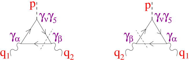
Figure 1: Diagrams describing $\langle\gamma(q_{1})\gamma(q_{2})|\bar{q}\gamma_{\nu}\gamma_{5}q|0\rangle$ and/or $\langle\gamma(q_{1})V(q_{2})|\bar{q}\gamma_{\nu}\gamma_{5}q|0\rangle$, with $p=q_{1}+q_{2}$. The cut corresponds to the calculation of the absorptive part in the variable $q_{2}^{2}$.

$t_{\nu\alpha\beta}$ is our basis for the spectral representation of $T_{\nu\alpha\beta}$ in terms of the variable $q_{2}^{2}$. The coupling at the vertex $\beta$ is $\gamma_{\beta}eQ_{q}$ if the particle 2 is a photon, and $-\gamma_{\beta}g(q_{2}^{2})/\sqrt{N_{c}}$ if it is a vector meson. The coupling $g(q_{2}^{2})$ will be further discussed below. By taking the trace and performing the integration over the internal momentum in the loop it is straighforward to obtain $t_{\nu\alpha\beta}$. The result is automatically gauge-invariant

$$q_{1}^{\alpha}t_{\nu\alpha\beta}(q_{1},q_{2})=0,\qquad q_{2}^{\beta}t_{\nu\alpha\beta}(q_{1},q_{2})=0.$$ (86)

It is therefore possible to write the covariant decomposition of $t_{\nu\alpha\beta}(q_{1},q_{2})$ in terms of three invariant amplitudes

$$t_{\nu\alpha\beta}(q_{1},q_{2}) = -p_{\nu}\epsilon_{\alpha\beta q_{1}q_{2}}ic_{0}+(q_{1}^{2}\epsilon_{\nu\alpha\beta q_{2}}-q_{1\alpha}\epsilon_{\nu q_{1}\beta q_{2}})ic_{1}$$ (88)

$${}+(q_{2}^{2}\epsilon_{\nu\beta\alpha q_{1}}-q_{2\beta}\epsilon_{\nu q_{2}\alpha q_{1}})ic_{2}.$$

This Lorentz structure is chosen in such a way that no kinematical singularities appear. We take $\gamma(q_{1})$ to be a real photon, $q_{1}^{2}=0$. Hence, the term containing the invariant amplitude $c_{1}$ does not contribute to the divergence of the current. Setting in addition $m_{q}=0$ one obtains for $c_{0}$ and $c_{2}$ with $s=q_{2}^{2}$

$$c_{0}(p^{2},s)=-\frac{\zeta(s)}{4\pi}\frac{s}{(s-p^{2})^{2}},\qquad c_{2}(p^{2},s)=-\frac{\zeta(s)}{4\pi}\frac{p^{2}}{(s-p^{2})^{2}},$$ (89)

where $\zeta(s)=2N_{c}Q_{q}^{2}\theta(s)$ for the $\gamma\gamma$ process and $\zeta(s)=-2\sqrt{N_{c}}Q_{q}g(s)\theta(s)$ for the $\gamma V$ process.

Clearly, the absorptive part $t_{\nu\alpha\beta}(q_{1},q_{2})$ of the axial-vector current matrix element respects the classical equation of motion, that is

$$p^{2}\,c_{0}(p^{2},s)-s\,c_{2}(p^{2},s)=0.$$ (90)

10 The triangle amplitude and its divergence

The full amplitude $T_{\nu\alpha\beta}(q_{1},q_{2})$ has the same Lorentz structure as its absorptive part

$$T_{\nu\alpha\beta}(q_{1},q_{2}) = -p_{\nu}\epsilon_{\alpha\beta q_{1}q_{2}}iC_{0}+(q_{1}^{2}\epsilon_{\nu\alpha\beta q_{2}}-q_{1\alpha}\epsilon_{\nu q_{1}\beta q_{2}})iC_{1}$$ (92)

$${}+(q_{2}^{2}\epsilon_{\nu\beta\alpha q_{1}}-q_{2\beta}\epsilon_{\nu q_{2}\alpha q_{1}})iC_{2}.$$

The absence of any contact terms in $T_{\nu\alpha\beta}$ can be verified by reducing out one of the photons and using the conservation of the electromagnetic current. The invariant amplitudes $C_{i}$ can be represented by the following dispersion integrals

$$C_{i}(p^{2},q_{1}^{2}=0,q_{2}^{2})=\frac{1}{\pi}\int_{0}^{\infty}\frac{c_{i}(p^{2},s)}{s-q_{2}^{2}-i0}ds.$$ (93)

All the integrals converge and thus need no subtraction.

Taking the divergence of $T_{\nu\alpha\beta}$ we find

$$ip^{\nu}T_{\nu\alpha\beta}=-\frac{1}{\pi}\left\{p^{2}\int_{0}^{\infty}\frac{c_{0}(p^{2},s)}{s-q_{2}^{2}}ds-q_{2}^{2}\int_{0}^{\infty}\frac{c_{2}(p^{2},s)}{s-q_{2}^{2}}ds\right\}\epsilon_{q_{1}\alpha q_{2}\beta}.$$ (94)

The form factor $G$ defined in Eqs. (80) and (82) now reads

$$G(p^{2},q_{2}^{2})=\frac{p^{2}}{4\pi^{2}}\int_{0}^{\infty}\frac{\zeta(s)}{(s-p^{2})^{2}}ds$$ (95)

In the case of the $\gamma\gamma$ process $\zeta(s)$ is a constant. The integral can be performed and gives the well-known value shown in Eq (81). In the case of the $\gamma V$ matrix element the integrals converge even better since $g(s)$ which appears in $\zeta(s)$ descibes the spatial size of the vector meson. We conclude from Eq. (95) that the divergence of the axial-vector current is nonzero for $m_{q}=0$ not only for the $\gamma\gamma$ but also for the $\gamma V$ final state! Namely,

$$G^{V}(p^{2},q_{2}^{2})=2\sqrt{N_{c}}eQ_{q}\frac{-p^{2}}{4\pi^{2}}\int_{0}^{\infty}\frac{g(s)}{(s-p^{2})^{2}}ds.$$ (96)

The behavior with respect to $p^{2}$ is however different from the $\gamma\gamma$ case and has the form $G^{V}(p^{2})\sim 1/p^{2}$ for the large values of $p^{2}$ where our formula applies.

For the transition to the $\gamma\rho$ (isospin-1) arising from the isovector axial current we obtain

$$G^{\rho}=(Q_{u}+Q_{d})\kappa\frac{f_{\rho}M_{\rho}}{p^{2}},\qquad\kappa=-\frac{\sqrt{N_{c}}}{4\pi^{2}}\frac{p^{4}}{f_{\rho}M_{\rho}}\int_{0}^{\infty}\frac{g(s)}{(s-p^{2})^{2}}ds.$$ (97)

The parameter $\kappa$ in this equation is non zero for $m_{q}=0$ and $|p^{2}|\to\infty$. $f_{\rho}$ is defined by the relation $\langle\rho^{-}|\bar{d}\gamma_{\nu}u|0\rangle=f_{\rho}M_{\rho}\epsilon^{*}_{\nu}$.

Eq. (97) takes into account the soft contribution to the form factor $G^{\rho}$. For large $|p^{2}|$ one should take care of the QCD evolution of the $\rho$-meson wave function from the soft scale $\mu^{2}\sim$ 1 GeV² to the scale $\mu^{2}\sim|p^{2}|$. This can be done most directly by expressing $\kappa$ in terms of the $\rho$-meson light-cone distribution amplitudes bb

$$\langle\rho(q_{2})|\bar{d}(x)\gamma_{\lambda}u(0)|0\rangle = -iq_{2\lambda}(\epsilon^{*}x)f_{\rho}M_{\rho}\int\limits_{0}^{1}due^{iuq_{2}x}\Phi(u)$$ (98)

$${}+\epsilon^{*}_{\lambda}f_{\rho}M_{\rho}\int\limits_{0}^{1}due^{iuq_{2}x}g_{\perp}^{(v)}(u),$$

$$\langle\rho(q_{2})|\bar{d}(x)\gamma_{\lambda}\gamma_{5}u(0)|0\rangle = -\frac{1}{4}\epsilon_{\lambda\eta\rho\sigma}\epsilon^{*\eta}q_{2}^{\rho}x^{\sigma}f_{\rho}M_{\rho}\int\limits_{0}^{1}due^{iuq_{2}x}g_{\perp}^{(a)}(u).$$ (99)

The diagrams of Fig 2 explain the procedure we follow: The quark propagator connects the axial current with the photon and the two distant space time points are bridged by the $\rho$ meson wave function. This leads to the following expression for $\kappa$

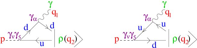
Figure 2: The diagrams for the matrix element $\langle\gamma(q_{1})\rho^{-}(q_{2})|\bar{d}\gamma_{\nu}\gamma_{5}u|0\rangle$, with two space time points bridged by the $\rho$ meson light-cone distribution amplitude.

$$\kappa=-\int\limits_{0}^{1}du\left[\frac{1+u}{4u^{2}}g_{\perp}^{(a)}-\frac{1-u}{u}g_{\perp}^{(v)}-\frac{1}{1-u}\Phi\right].$$ (100)

The leading-twist distribution amplitudes

$$g_{\perp}^{(a)} = 6u(1-u),$$

$$g_{\perp}^{(v)} = \frac{3}{4}\left(1+(2u-1)^{2}\right),$$

$$\Phi = \frac{3}{2}u(1-u)(2u-1)$$ (101)

give the main contribution for large $p^{2}$ and lead to the value $\kappa=-3/2$. Corrections to this value are calculable in terms of the higher twist distribution amplitudes bb .

Summing up, our results are as follows:

1. The divergence of the axial vector current and thus the form factor $G$ does not vanish in the limit $m_{q}\to 0$. This holds for the $\gamma\rho$ final state as well as for the $\gamma\gamma$ final state. The observed effect for vector mesons requires a proper modification of the equation of motion for the axial current. For large momenta $p$ of the axial-vector current the corresponding ’bound state anomaly’ can be described in terms of a non-local operator appearing at order $e$ (there are no local operators of the appropriate dimension):

   $${\rm Single\;flavor\;current}:$$

   $$\partial^{\nu}(\bar{q}\gamma_{\nu}\gamma_{5}q)=2im\;\bar{q}\gamma_{5}q+\frac{(eQ_{q})^{2}N_{c}}{16\pi^{2}}F\tilde{F}$$ (102)

   $${}+e\kappa\,Q_{q}\,\Box^{-1}\left\{\partial_{\mu}(\bar{q}\gamma_{\nu}q)\cdot\tilde{F}^{\mu\nu}\right\}+O(\Box^{-2}).$$ (103)

   $${\rm Isovector\;charged\;current}:$$

   $$\partial_{\nu}(\bar{d}\gamma_{\nu}\gamma_{5}u)=i(m_{u}+m_{d})\bar{u}\gamma_{5}d-ie(Q_{u}-Q_{d})\bar{u}\gamma_{\nu}\gamma_{5}d\cdot A^{\nu}$$

   $${}+e\kappa\frac{(Q_{u}+Q_{d})}{2}\Box^{-1}\left\{\partial_{\mu}(\bar{u}\gamma_{\nu}d)\cdot\tilde{F}_{\mu\nu}\right\}+O(\Box^{-2}).$$ (104)

   $\kappa$ can be expanded in a power series of $\alpha_{s}$. In leading order one obtains the value $\kappa=-3/2$.

   As pointed out in bmns , the $\rho\gamma$ anomaly is important in rare decays: for instance, in $B\to\rho\gamma$ decays, it substantially corrects the weak annihilation amplitude which carries the CP violating phase.

2. The amplitude for the $\rho\rho$ final state also stays finite for $m_{q}=0$. The corresponding non-local anomalous term for the divergence of the isovector axial current $\partial_{\nu}(\bar{q}\gamma_{\nu}\gamma_{5}{\tau^{a}}q)$ appears already at order $O(e^{0})$. The operator structure of the anomalous term is more complicated in this case. One of the possible lowest-dimension operators which has a nonvanishing $\langle\rho\rho|...|0\rangle$ matrix element and thus will contribute to the anomalous term (in leading order in $1/p^{2}$) is the product of the two isovector tensor currents

   $$\epsilon^{abc}\epsilon^{\mu\nu\alpha\beta}\Box^{-1}\left(\bar{q}\sigma_{\mu\nu}{\tau^{b}}q\cdot\bar{q}\sigma_{\alpha\beta}{\tau^{c}}q\right).$$ (105)

   Accordingly, for large $|p^{2}|$ the $\langle\rho\rho|...|0\rangle$ amplitude of the divergence of the axial-vector current is given by the factorized matrix element of the anomalous term and has a $1/p^{2}$ suppression

   $$\begin{array}[]{rcl}\langle\rho(q_{1})\rho(q_{2})|\partial^{\nu}(\bar{d}\gamma_{\nu}\gamma_{5}u)|0\rangle&=&\epsilon_{q_{1}\epsilon^{*}_{1}q_{2}\epsilon^{*}_{2}}G^{\rho\rho},\\ G^{\rho\rho}&\sim&f_{\rho}^{2}/p^{2}+O(1/p^{4}).\end{array}$$ (106)

3. We have illustrated the appearance of non-local anomaly due to vector mesons in QCD. This anomaly is of a general nature and should be present in any theory containing $J^{P}=1^{-}$ bound states. For example, the anomaly will also contribute to the generation of orthopositronium by the leptonic axial-vector current. In contrast to the conventional local anomalies, there is no obvious cancellation of the non-local anomalies in the standard model.

*Could there be a Fourth Generation?We would like to thank David Sutherland for discussions and useful remarks. C.D. FroggattE-mail: c.froggatt@physics.gla.ac.uk and J.E. DubickiE-mail: j.dubicki@physics.gla.ac.uk

11 Introduction

Despite the success of the Standard Model (SM), it is far from complete. For instance, the origin of the inter-generation mass hierarchy and issues such as baryon asymmetry are yet to be resolved. We would expect new physics to contribute to these areas. At the more fundamental level, nobody knows of any deep explanation as to why there should only be three generations of quarks & leptons. For these reasons, and others, extensions of the three-generation SM are being investigated. We investigate the possibility of incorporating a fourth-generation into a GUT model.
As is well known, all fourth-generation models must adhere to certain experimental constraints, the first of which stems from precise measurements of the decay characteristics of the $Z$-boson performed at LEP. This has set a lower bound of $M_{F}\geq\frac{M_{Z}}{2}$ on any non-SM particles that couple to the $Z$-boson. Ignoring for the moment the unnatural hierarchy emerging within the neutrino sector, we assume a Dirac mass $\sim\left(\frac{M_{Z}}{2}\right)$ for the heavy neutral lepton. We label the fourth-generation doublets explicitly as,

$$Q_{4}={\left(\begin{array}[]{c}T\\ B\end{array}\right)}_{4}\quad T_{4}^{c}\quad B_{4}^{c};\qquad L_{4}={\left(\begin{array}[]{c}N\\ E\end{array}\right)}_{4}\quad N_{4}^{c}\quad E_{4}^{c}$$

Physics beyond the Standard Model is severely constrained by precision electroweak data. Assuming SM contributions, fits to LEP data give the radiative correction parameter $S=-0.04\pm 0.11$. For a heavy ($\gg M_{Z}$) degenerate fourth-generation we obtain $\Delta S=\frac{2}{3\pi}$ and so is ruled out at $99.8\%$ $C.L$. However, Maltoni et al. maltoni have shown that particles with mass $M\sim\frac{M_{Z}}{2}$ give drastically different contributions to $S$. It is possible for a heavy neutrino $N$ with mass $M_{N}\sim\frac{M_{Z}}{2}$ to cancel the contributions from the heavy $T,B,E$ with the SM solution

$$M_{E}>M_{N};\quad M_{T}>M_{B}$$

$$M_{N}\sim\frac{M_{Z}}{2};\quad M_{B}=M_{B}^{min}$$

$$(M_{E}-M_{N})\sim 3(M_{T}-M_{B})\sim 60GeV$$ (107)

and the $N$ must be relatively stable to avoid detection (i.e. mixing matrix elements $V_{Ne,\mu,\tau}<10^{-6}$). An extra generation can be accomodated below the $1\sigma$ level (or even two generations at $1.5\sigma$). However, it was shown by Gunion et al. gunion that the fourth-generation charged lepton must be relatively light ($<$ 60 GeV) in order to stay in the perturbative regime below the GUT scale. Although they worked within a supersymmetric framework, similar results are expected to hold in the SM pirogov . Decreasing $M_{E}$ below $\sim$ 60 GeV to achieve perturbative unification is not consistent with the above SM fits (Eq.(107)) to the precision data. Therefore, we require the cancellations to arise from another sector and so we consider a supersymmetric theory. Indeed, it is shown in  maltoni that light supersymmetric particles can also effect the fit to precision data, allowing for a fourth-generation below the $2\sigma$ level. In particular, neutralinos (${\tilde{\chi}}^{0}_{1}$) and charginos (${\tilde{\chi}}^{\pm}_{1}$) with masses $<M_{Z}$ can provide the correct sign contributions whilst being consistent with current experimental limits if nearly degenerate L3 .
In this paper we investigate the possibility of consistently incorporating a fourth-generation into a $N=1$ R-parity conserving supergravity model. We assume a structure akin to that of the minimal supersymmetric standard model (MSSM3), adding a complete chiral fourth-generation and its associated SUSY partners (the so called MSSM4). Specifically we require $(i)$ perturbative values for all Yukawa couplings at energies up to the GUT scale and $(ii)$ gauge coupling unification. These two constraints will be termed collectively as perturbative unification.
Having satisfied precision data fits, it remains for us to provide solutions that $(i)$ unify perturbatively at the GUT scale and $(ii)$ evade the direct experimental searches performed at $CDF$. In section 12 we investigate the specific decay channels of the fourth-generation quarks and ensure we can provide consistency with the experimental direct searches. The solution we present requires the introduction of light SUSY particles ($M_{{\tilde{\chi}}^{0}},M_{{\tilde{\chi}}^{\pm}},M_{\tilde{B}}$), so the two-body decays $T\rightarrow\tilde{B}{\tilde{\chi}}^{+}$ and $B\rightarrow\tilde{B}{\tilde{\chi}}^{0}$ are kinematically allowed. These will always dominate over the one-loop FCNC decays $B\rightarrow bZ^{0}$ and two-generation decays $B\rightarrow cW^{-}$ that traditional searches have looked for, whilst at the same time suppress the decay rate $T\rightarrow bW^{+}$. We note a light, degenerate chargino/neutralino pair is just what is needed to provide the necessary cancellations in precision data.
In section 13 we discuss the influence of specific fourth-generation/SUSY masses on precision data fits in more detail and point out new features that appear when trying to satisfy all constraints. In section 14 we proceed with a renormalisation group study of the four generation MSSM. Under the assumption of a common mass scale for the coloured/weak sparticle spectrum ($M_{col}$/$M_{wk}$ respectively) we will derive upper bounds on $M_{col}$. This bound stems from the fact that if we are to achieve perturbative values for the top quark Yukawa coupling constant $h_{t}$ up to the GUT scale, then the effects of the coloured sparticle spectrum must be included in the running of the strong coupling $\alpha_{3}$ at an early stage. Finally, in section 15 we investigate the lightest Higgs mass in the MSSM4.

12 Experiment and a Fourth Generation

In this study we assume the hierarchy within the fourth generation is such that $M_{T}>M_{B}$ and $M_{E}>M_{N}$. We begin our discussion by considering the leptonic sector. Under the assumption that the mixing between ($E,N$) and the first three generations is negligible, the decay $E\rightarrow NW^{*}$ will be dominant. In order to evade experimental bounds, the mass difference $\Delta M_{L}=M_{E}-M_{N}$ must be small enough to result in a virtual $W^{*}$ whose decay products are too soft to be triggered. Regarding the heavy neutrino, LEPII has set the bound $M_{N}>$ 70 - 80 GeV based on the search for $N\rightarrow lW^{*}$ ($l=e,\mu$ or $\tau$) where the mixing matrix elements $V_{Ne,\mu,\tau}>10^{-6}$ lepton . A heavy neutrino with this mass is inconsistent with perturbative unification. However, we have previously assumed that the mixing of the fourth generation leptonic sector is in fact negligible ($V_{Ne,\mu,\tau}<10^{-6}$) so the neutrino is stable enough to leave the detector and in this case only the DELPHI bound of $M_{N}>$ 45 GeV from measurements of the $Z$-width applies. From figure (4) in lepton we can see that $M_{E}\sim M_{N}\sim$ 50 GeV is allowed.
Turning to the quark sector, the requirement of perturbative unification places strict upper limits on the masses of the $T$ and $B$ and they certainly must be below the top quark whose mass is $M_{t}=174\pm$ 5.1 GeV. Experimental searches for the fourth-generation quarks have mainly concentrated on the $B$-quark where CDF have set a bound of $M_{B}>$ 199 GeV assuming the branching ratio $BR(B\rightarrow bZ^{0})\sim 1$. The search is also sensitive to other decay modes; for instance the decay $B\rightarrow bh^{0}$ or $B\rightarrow cW^{-}$ is triggered as long as $BR(R\rightarrow bZ)$ is not negligible, since the hadronic decay of the $h^{0}$ or $W$ are kinematically similar to those of the $Z$. One possible escape might come about if we note that $h^{0}\rightarrow N\overline{N}$ would compete with $h^{0}\rightarrow b\overline{b}$ for $M_{h}^{0}\sim M_{Z}^{0}$ (dominating for larger $M_{h}^{0}$) and would provide an invisible signature. For $M_{B}\sim$ 100 GeV and $M_{h}^{0}\sim M_{Z}^{0}$ we would also expect $BR(B\rightarrow bh^{0})\sim BR(B\rightarrow bZ^{0})$ hou . However, CDF still exclude a $B$-mass in the range 104 GeV $\rightarrow$ 152 GeV assuming $BR(B\rightarrow bZ^{0})\geq 50\%$ and no sensitivity to the other decay modes quark . Taking $M_{h^{0}}\sim$ 100 GeV (which places $M_{B}\sim$ 105 GeV for $B\rightarrow bh^{0}$ to be kinematically allowed) we obtain $BR(h^{0}\rightarrow invisible)\sim 80\%-90\%$ and so we can expect to rule this possibility out. Moreover, we have yet to account for the $T$ decays which turn out to be highly constrained if we assume $SM$-like processes. The channel $T\rightarrow bW^{+}$ is prohibited for the obvious reason that the $T$-quark would have been picked up in the $CDF$ search for the top quark. Although we might assume that $T\rightarrow BW^{*}$ is dominant by suppressing $V_{Tb}$ we must notice that, since the $T\overline{T}$ production cross-section is similar to that of $B\overline{B}$, we would effectively expect double the event rate on the $B$-quark search. Taking this into account would further strengthen existing bounds on the $B$-quark mass.
From the ideas presented so far we might conclude that the fourth-generation with perturbative unification is not consistent with experimental bounds on the ($T,B$) quarks. We have not, however, considered the possibility of light SUSY particles providing decay channels for ($T,B$). In this situation one can constrain the light (i.e. $<M_{Z}$) neutralino/chargino pair, which is already required by fits to precision data, in order to provide the following two-body decays

$$T\rightarrow\tilde{B}{\tilde{\chi}}^{\pm}_{1};\quad B\rightarrow\tilde{B}{\tilde{\chi}}^{0}_{1}$$ (108)

Ensuring both decay channels are kinematically accessible, combined with the fact that perturbative unification requires(for $M_{t}=$ 170 GeV) $M_{Q}<$ 110 GeV, where $M_{Q}=M_{B}\simeq M_{T}$, places severe restrictions on the allowed spectrum. To be definite we choose
$\displaystyle M_{\tilde{\chi}}$ $\displaystyle\simeq$ $\displaystyle 50\;GeV$ $\displaystyle M_{\tilde{B}}$ $\displaystyle\simeq$ $\displaystyle 55\;GeV$ $\displaystyle M_{Q}$ $\displaystyle\simeq$ $\displaystyle 105-107\;GeV$ $\displaystyle M_{t}$ $\displaystyle=$ $\displaystyle 170\;GeV$
where under the assumption of a nearly degenerate neutralino/chargino pair we define the notation $\Delta M_{\tilde{\chi}}=M_{{\tilde{\chi}}^{\pm}_{1}}-M_{{\tilde{\chi}}^{0}_{1}}$; $M_{\tilde{\chi}}=M_{{\tilde{\chi}}^{0}_{1}}\sim M_{{\tilde{\chi}}^{\pm}_{1}}$. Although these masses seem to be contrived, we note that they can be obtained from reasonable assumptions about the supersymmetric sector. In order to obtain $\Delta M_{\tilde{\chi}}\sim M_{{\pi}^{+}}$ we require the hierarchy $|\mu|\gg M_{1}\geq M_{2}$ where $|\mu|$ is the Higgs mixing parameter and is fixed by the requirement of radiative electroweak breaking. $M_{1}$ and $M_{2}$ are the electroweak gaugino masses (for a review of supersymmetry see susy ). This structure can occur naturally when the gaugino masses are dominated by loop corrections, originating from superstring models (i.e. the $O-II$ model string ). We also require substantial ${\tilde{B}}_{L}/{\tilde{B}}_{R}$ mixing to induce the light $\tilde{B}$ mass.

13 Precision Measurements and a Fourth Generation

It is difficult to provide bounds from precision data without a fully consistent study taking into account exact particle masses, any light SUSY spectra present and mixings between different flavours. However, it is pointed out in maltoni that a highly degenerate neutralino/chargino pair ($\Delta M_{\tilde{\chi}}\sim M_{{\pi}^{+}}$; $M_{\tilde{\chi}}\sim$ 60 GeV) can provide the necessary contributions needed to cancel that of the fourth- generation whilst at the same time being consistent with LEP bounds. Looking at their results, we see that the magnitude of the contribution to the fitted parameters from this sector is highly dependent on $M_{\tilde{\chi}}$. Indeed, demanding $M_{\tilde{\chi}}\simeq$ 50 GeV in our model might be too restrictive. One possible solution presents itself if we assume that the lightest supersymmetric particle (LSP) is in fact the fourth-generation sneutrino $\tilde{N}$. We have no phenomenological bounds on this scenario, the ${\tilde{\chi}}^{0}_{1}$ would decay invisibly via ${\tilde{\chi}}^{0}_{1}\rightarrow{\upsilon}_{\tau}\tilde{N}$ assuming the $3-4$ mixing angle is non-zero gunion . This does, however, allow us to increase $M_{\tilde{\chi}}$ whilst decreasing $M_{\tilde{B}}$. The following masses are possible
$\displaystyle M_{\tilde{\chi}}$ $\displaystyle\simeq$ $\displaystyle 55\;GeV$ $\displaystyle M_{\tilde{B}}$ $\displaystyle\simeq$ $\displaystyle 50\;GeV$ $\displaystyle M_{\tilde{N}}$ $\displaystyle\simeq$ $\displaystyle 46\;GeV$ $\displaystyle M_{Q}$ $\displaystyle\simeq$ $\displaystyle 105-107\;GeV$ $\displaystyle M_{t}$ $\displaystyle=$ $\displaystyle 170\;GeV$
The sneutrino $\tilde{N}$ is now the LSP and is stable due to $R$-parity. The bottom squark will decay via $\tilde{B}\rightarrow ij\tilde{N}$ (where $(i,j)=(c,\tau)$ or $(b,\upsilon_{\tau})$) depending on which decay is kinematically allowed. Such decays involve the factor $V_{Bi}V_{Nj}$, leading to a long lifetime. If the coupling of $\tilde{N}$ to the $Z$-boson is small then it is possible to have $M_{\tilde{N}}<\frac{M_{Z}}{2}$. This allows us to decrease $M_{\tilde{B}}$ even further, hence increase $M_{\tilde{\chi}}$ and still retain the decay channels in Eq.(108). The maximum value obtained in this case is $M_{\tilde{\chi}}^{max}\leq$ 60 GeV, consistent with precision fits as shown in maltoni .
The fits to precision data performed in maltoni were for a different set of fourth-generation masses. Although the non-universal contributions (see Maltoni, Ph.D. thesis maltoni for terminology) remain the same in the limit $|M_{i}-M_{j}|\ll M_{Z}$ (where $i,j$ label the two fermions within the same $SU(2)_{L}$ doublet), the universal contributions will differ. However, we could arrange to have significant $SU(2)_{L}$ breaking in the ${(\tilde{T},\tilde{B})}_{L}$ doublet if $M_{\tilde{T}}$ was found to be sufficiently large. This would provide universal contributions to the precision parameters maltoni , thus compensating for the difference between our model with highly degenerate fourth-generation fermion doublets and the fits as performed in maltoni .

14 Renormalization Group Study of the MSSM4

Here we investigate the effect of the fourth-generation on the evolution of couplings to the GUT scale, where we require gauge coupling unification. This places upper limits on the masses of the extra particles to ensure their Yukawa couplings run perturbatively to the unification scale $M_{U}$ ($h^{2}(\mu)\leq 4\pi$, $M_{Z}\leq\mu\leq M_{U}$). Starting at the low-energy scale $M_{Z}$, the electroweak gauge couplings $\alpha_{1}(M_{Z})$, $\alpha_{2}(M_{Z})$ are fixed through the relations $\frac{1}{\alpha_{i}(M_{Z})}=\frac{3}{5}\frac{\left(1-{\sin^{2}\theta_{W}}\right)}{\alpha_{em}(M_{Z})};\frac{{\sin^{2}\theta_{W}}}{\alpha_{em}(M_{Z})}$ for $i=1,2$ respectively. The strong coupling $\alpha_{3}(M_{Z})$ is taken from the Particle Data Group (PDG) pdg to be $0.1181\pm 0.002$. We take the best fit values for $\frac{\alpha_{em}(M_{Z})}{\sin\theta_{W}}$ from the PDG. In principle, one should extract the $Z$-pole couplings assuming the full MSSM4, thereby accounting for the fourth-generation fermions and light SUSY spectra in a fully consistent way. We have also performed our study in the $\overline{MS}$ scheme although it is the $\overline{DR}$ scheme that is consistent with supersymmetry. However, differences between the $\overline{DR}$ and $\overline{MS}$ schemes are not significant at the low-energy scale as compared to other uncertainties.

In our analysis we neglect all Yukawa couplings from the first three generations except that of the $t$-quark whose mass we take to be $M_{t}^{pole}=$ 170 GeV. As is typical with four-generation models, we require small values of $\tan\beta$ (the ratio of the Higgs vev’s) so as to avoid $h_{B}(M_{Z})\geq$$\cal O$($\sqrt{4\pi}$). Once all couplings at $M_{Z}$ have been fixed, we integrate up in energy scale using the two-loop renormalization group equations (RGE). The one-loop leading logarithmic threshold corrections from the SUSY sector are accounted for in the numerical procedure. We select the point where $\alpha_{1}(\mu)=\alpha_{2}(\mu)$ as the unification scale $M_{U}$ with coupling $\alpha_{U}(M_{U})$. Any deviation in $\alpha_{3}(M_{U})=\alpha_{U}(M_{U})$, which we parameterize as $\delta=\frac{\alpha_{3}(M_{U})-\alpha_{U}(M_{U})}{\alpha_{U}(M_{U})}$, can arise from either of two sectors. On the one hand, we have the $\overline{MS}$ vs. $\overline{DR}$ mismatch, experimental errors in $\alpha_{em}(M_{Z})$/$\sin\theta_{W}$ and the variations in the best fit values of $\alpha_{em}(M_{Z})$ and $\sin\theta_{W}$ as the fourth-generation and light SUSY particles ($\tilde{M}<M_{Z}$) are included. However, more importantly, assuming no intermediate scales, high-energy threshold corrections from specific GUT/string models can provide contributions to $\delta$. Following ross , we note that these corrections (for particular models)can be large. Considering all the uncertainties together, we conservatively require unification to within $\pm 5\%$ ($\delta=\pm 0.05$).
The SUSY threshold corrections in the MSSM4 are important as they can influence whether or not a particular set of masses ($M_{t},M_{T},M_{B},M_{N},M_{E}$) will retain perturbative consistency to the GUT scale. This can be observed analytically if we write the one-loop leading logarithmic correction to the strong coupling from the SUSY sector

$$\frac{1}{\alpha_{3}^{+}(M_{Z})}-\frac{1}{\alpha_{3}^{-}(M_{Z})}=\frac{b_{3}^{MSSM4}-b_{3}^{SM4}}{2\pi}\ln\left(\frac{M_{col}}{M_{Z}}\right)$$ (109)

where $M_{col}$ represents an effective threshold scale and $b_{3}^{MSSM4/SM4}$ represents the one-loop beta function contribution to the strong coupling in the MSSM4/SM4 respectively. This correction is implemented at the scale $M_{Z}$ and accounts for the coloured sparticles with masses $M_{col}>M_{Z}$ in the running of the strong coupling. $\alpha^{+}$/$\alpha^{-}$ represents the renormalized gauge coupling just above/below the scale $M_{Z}$. Eq.(109) holds if the masses of the sparticles are $\leq$ 2 TeV polonsky . It is obvious that the higher the scale $M_{col}$, the lower $\alpha_{3}^{+}(M_{Z})$. Looking at the structure of the RGE it is evident that the strong coupling plays an important role in keeping the Yukawa couplings perturbative. We obtain an upper bound $M_{col}^{max}$, above which the initial $\alpha_{3}$ is too small to counteract the effect of the fourth-generation couplings.
In practice, we perform a full numerical study, accounting for the threshold corrections from $t,T,B,{\tilde{M}}_{i}$ (where i runs over all sparticles with $\tilde{M}>M_{Z}$) by changing the $\beta$-functions and using the step-function approach in the running of the gauge couplings boer . We assume separate degeneracies amongst the coloured and weak SUSY spectrum

$$M_{wk} = |\mu|=M_{\tilde{L}}=M_{\tilde{H}}=M_{\tilde{W}}=M_{H}$$ (110)

$$M_{col} = M_{\tilde{Q}}=M_{\tilde{g}}$$

We take the fixed value $M_{wk}=$ 500 GeV though in principle it could be anywhere up to $\sim$ 1 TeV. Of course, considering separate degeneracies amongst the coloured and weak sparticle spectra is an approximation. In fact, our model demands the introduction of light sparticles to ensure consistency with experimental searches for the fourth-generation and precision data bounds, thus providing significant deviations from degeneracy. Nevertheless, the study does serve to show that the combined effect of the coloured spectrum is bounded from above in the process of retaining perturbative consistency of the model. See figure 3 for a plot of $M_{col}^{max}$ vs. $\tan\beta$. In particular we conclude that perturbative unification is only possible for the small range $1.5<\tan\beta<1.7$. Further restrictions on the allowed $\tan\beta$ range arise from the mass of the lightest Higgs boson that must exceed its experimental lower bound (see section 15).

Figure 3: Plot of $M_{col}^{max}$ vs. $\tan\beta$ for $M_{T}=$ 107 GeV; $M_{B}=$ 105 GeV; $M_{N}=$ 46 GeV; $M_{E}=$ 50 GeV; $M_{t}=$ 170 GeV.

15 The Higgs Sector of the MSSM4

The effect of the fourth-generation on the lightest Higgs mass ($M_{h}$) is investigated. For our particular solution of ($M_{t},M_{T},M_{B},M_{N},M_{E},{\tilde{M}}_{i}$) that is consistent with perturbative unification, we see the upper bound $M_{h}^{max}$ increases through loop corrections from the extra particles. Normally, the Higgs sector of minimal supersymmetry models is fixed by two parameters $(i)\tan\beta$ and $(ii)M_{A}$ (the pseudoscalar Higgs mass). We fix $\tan\beta\sim 1.63$ from the requirement of perturbative unification (see figure 3) and so we are left with the one free parameter $M_{A}$. Assuming this is to be included in the heavy Higgs sector ($M_{H}$) we vary 500 GeV $\leq|\mu|=M_{A}\leq$ 1 TeV to be consistent with Eq.(110).
In the MSSM4, for $M_{h}\geq$ 100 GeV, the channel ($h\rightarrow\mbox{invisible}$), where invisible represents ($N\overline{N},E\overline{E},\tilde{N}\overline{\tilde{N}},\tilde{\chi}\overline{\tilde{\chi}}$), will open and would dominate over conventional $h\rightarrow b\overline{b}$ rates. Exclusion limits will now come from the missing energy search ($e^{+}e^{-}\rightarrow Zh\rightarrow Z+\mbox{missing energy}$) that currently sets the lower bound at 114.4 GeV invisible . We therefore need to check, for our constrained set of parameters ($M_{T},M_{B},M_{N},M_{E},{\tilde{M}}_{i},\tan\beta$), that $M_{h}^{max}$ falls above this experimental lower bound. We shall employ the one-loop effective potential with contributions from the top/stop and fourth-generation fermions/sfermions. Since we are at low $\tan\beta$ we can ignore the contributions from the third generation bottom/sbottom masses.
In general, the sfermion mass matrix can be written as

$$M_{\tilde{i}}=\left(\begin{array}[]{cc}M_{Si}^{2}+M_{i}^{2}+\Delta_{Di}&M_{i}\left(A_{i}-\mu\cot\beta\right)\\ M_{i}\left(A_{i}-\mu\cot\beta\right)&M_{{\overline{S}}i}^{2}+M_{i}^{2}+\Delta_{{\overline{D}}i}\end{array}\right)$$

where $\Delta_{D}$ and $\Delta_{\overline{D}}$ represents the $D$-term contributions. We set the soft supersymmetry breaking parameters for the coloured squarks $M_{Si}=M_{{\overline{S}}i}=M_{col}$ ($i=t,T,B$) and, for a given $\tan\beta$, we vary $M_{col}$ within the range as plotted in figure 3. For the sleptons $M_{Si}=M_{{\overline{S}}i}=|\mu|$ ($i=E,N$). We randomly vary the mixing parameters ($A_{t},A_{T},A_{B},A_{N},A_{E}$) and retain the maximum value returned for the lightest Higgs mass. As shown in previous studies of the Higgs sector, this will occur for $A\sim\sqrt{6}M_{col}$. Large mixings will induce light sparticles ($<M_{Z}$) which are required in the MSSM4 to provide the decay channels to the fourth-generation quarks. Since we are at low $\tan\beta$ ($\sim 1.63$) we require relatively heavy squarks in order to increase the Higgs mass above its experimental lower bound. We find that $M_{h}^{max}>$ 114 GeV for $M_{col}\geq$ 350 GeV. This is consistent with results from section 14. The absolute upper bound (that occurs when $M_{col}=$ 500 GeV) is $M_{h}^{abs}\sim$ 120 GeV.

16 Conclusions

We have seen that it is possible to incorporate a fourth-generation into a GUT model, requiring the existence of supersymmetric particles in order to provide the necessary cancellations in precision fits. We constrain the fourth-generation masses to be $M_{T}=$ 107 Gev; $M_{B}=$ 105 GeV; $M_{N}=$ 46 GeV; $M_{E}=$ 50 GeV. The MSSM4 SUSY spectrum needs to be relatively light in order to retain perturbative consistency to the unification scale ($M_{col}\leq$ 500 GeV). On the other hand ($M_{col}\geq$ 350 GeV) is set from the requirement that the lightest Higgs mass must be above its present experimental lower bound. In order to provide decay channels to the fourth-generation quarks, it might be that the LSP is the sneutrino $\tilde{N}$. This has implications for dark matter constraints. The SUSY spectrum needed to satisfy all constraints can not be obtained from MSUGRA scenarios with universal parameters at the unification scale.

*Another Complex Bateman Equation D. B. FairlieE-mail:david.fairlie@durham.ac.uk

17 Introduction

This paper is another in a series devoted to an investigation of simple equations exhibiting covariance of solutions. These equations have arisen in the study of generalisations of the Bateman equation gov , in the equations arising from continuations of the String and Brane Lagrangians to the situation where the target space has fewer dimensions than the base space baker and a complex form of these equations fai . The simplest example of these is a complexification of the Bateman equation. What we have called the Complex Bateman equation is the following equation for a real function $\phi$ defined over the space of variables $(x_{1},\ x_{2};\ \bar{x}_{1},\ \bar{x}_{2})$;

$$\phi_{x_{1}}\phi_{\bar{x}_{1}}\phi_{x_{2}\bar{x}_{2}}+\phi_{x_{2}}\phi_{\bar{x}_{2}}\phi_{x_{1}\bar{x}_{1}}-\phi_{x_{1}}\phi_{\bar{x}_{2}}\phi_{\bar{x}_{1}x_{2}}-\phi_{x_{2}}\phi_{\bar{x}_{1}}\phi_{x_{1}\bar{x}_{2}}\,=\,0.$$ (111)

(Here subscripts denote differentiation). This equation was shown to be completely integrable chaundy leznov , with solution given by solving for $\phi$ the following constraint upon two arbitrary functions of three variables, $F,\ G$;

$$F(\phi;\,x_{1},x_{2})\,=\,G(\phi;\,\bar{x}_{1},\bar{x}_{2}).$$

From the form of the solution, or from the equation itself, it is manifest that if $\phi$ is a solution, any function of $\phi$ will also be a solution and thus that the equation exhibits covariance. It is also invariant under separate diffeomorphisms of the pairs of variables $(x_{1},\ x_{2})$ and $(\bar{x}_{1},\ \bar{x}_{2})$. In fact a subclass of solutions is given by the sum of ‘holomorphic’ and ‘antiholomorphic’ functions

$$\phi\,=\,f(x_{1},x_{2})+g(\bar{x}_{1},\bar{x}_{2}).$$

A general characteristic of such equations is that they possess an infinite number of inequivalent Lagrangians. The equations of motion are partially, or sometimes fully solveable in implicit form, as in the examples cited. The fully integrable eqautions arise from kinematical first order equations of hydrodynamic type.

18 Another Complex Bateman Equation

Now there is another possibility for complexification; we could take instead

$$\bar{\phi}_{x}\phi_{x}\phi_{tt}-\bar{\phi}_{x}\phi_{t}\phi_{tx}-\bar{\phi}_{t}\phi_{x}\phi_{tx}+\bar{\phi}_{t}\phi_{t}\phi_{xx}\,=\,0,$$ (112)

together with its complex conjugate. These equations also exhibit covariance; $\phi$ may be replaced by any function of itself, and the same for $\bar{\psi}$ and the equations remain invariant. Where do these equations come from? Take the hydrodynamic equations

$$\frac{\partial u}{\partial t} = v\frac{\partial u}{\partial x},$$ (113)

$$\frac{\partial v}{\partial t} = u\frac{\partial v}{\partial x},$$ (114)

and set $\displaystyle{u\,=\,\frac{\bar{\phi}_{t}}{\bar{\phi}_{x}},\ v\,=\,\frac{\phi_{t}}{\phi_{x}}}$, and the equation (112), together with its complex conjugate are reproduced. Indeed, all that is necessary is to set in an alternative reduction, $u=\bar{\phi}$ and $v=\phi$ and the same equations arise in consequence. These equations admit an infinite number of conserved quantities mulvey ; If $S_{n}$ denotes the symmetric polynomial of degree $n$ in $u,\ v$, then

$$\frac{\partial}{\partial t}S_{n}\,=\,\frac{\partial}{\partial x}(uvS_{n-1})$$ (115)

is a conservation law. This is easily proved by induction and from the iterative definition: $S_{n}\,=\,u^{n}+vS_{n-1}$. These equations can be integrated by the usual hodographic method of interchanging dependent and independent variables, where they become

$$\frac{\partial x}{\partial v} + v\frac{\partial t}{\partial v}\,=\,0,$$ (116)

$$\frac{\partial x}{\partial u} + u\frac{\partial t}{\partial u}\,=\,0,$$ (117)

which can be solved in terms of two arbitrary functions $f,\ g$ to give

$$t\,=\,f^{\prime}(u)+g^{\prime}(v);\ \ \ x\,=\,f(u)-uf^{\prime}(u)+g(v)-vg^{\prime}(v)$$

with primes denoting differentiation with respect to the argument. If $u=\bar{\phi}$ and $v=\phi$ this parametrisation is a solution to the alternative complexification. Note that the requirements that $(t,\ x)$ be real imposes a further constraint upon the functions $(f,\ g)$. Of course, if $(\phi,\ \bar{\phi})$ are treated as independent real functions, no such restriction exists. Now the second order equations (112) are Poincaré invariant; indeed are covariant under general inhomogeneous linear transformations of the independent variables. This must be true also for the first order equations (116), (117). They are clearly translation invariant; if $(t,\ x)$ transform as

$$t^{\prime}\,=\,at+bx,\\ \ x^{\prime}\,=\,ct+dx,$$

then invariance will be maintained if

$$u^{\prime}\,=\,\frac{du-c}{a-bu},\ \ \ \ v^{\prime}\,=\,\frac{dv-c}{a-bv}.$$

19 2-dimensional Born-Infeld equation

We may remark parenthetically that the same equations(113),(114) also yield the general solution to one form of the so-called Born-Infeld equation in two dimensions in light-cone co-ordinates mulvey arik ;

$$\phi_{x}^{2}\phi_{tt}+\phi_{x}^{2}\phi_{tt}-(\lambda+2\phi_{x}\phi_{t})\phi_{xt}\,=\,0.$$

This is achieved by setting

$$\frac{\partial\phi}{\partial x}\,=\,\frac{\sqrt{\lambda}}{\sqrt{u}-\sqrt{v}},\ \ \ \frac{\partial\phi}{\partial t}\,=\,\frac{\sqrt{\lambda uv}}{\sqrt{u}-\sqrt{v}}.$$

The integrability constraints upon these equations is just the Born-Infeld equation itself. Thus the primacy of the first order hydrodynamic equations is again manifest. This is a phenomenon which has been noticed before; that the same first order equations yield different second order ones depending upon the assumptions made about the dependency of the unknown functions in the first order equations upon the functions which enter into the second order equations intrev fai .

20 Lagrangian

The construction of a Lagrangian for (112) follows along the lines of fai . Introduce an auxiliary field $\psi$ and consider the singular Lagrangian

$${\cal L}\,=\,\left(\frac{\partial\bar{\phi}}{\partial t}\frac{\partial\psi}{\partial x}-\frac{\partial\psi}{\partial t}\frac{\partial\bar{\phi}}{\partial x}\right)\frac{\frac{\partial\phi}{\partial t}}{\frac{\partial\phi}{\partial x}}.$$ (118)

The equation of motion corresponding to variations in the field $\psi$ is simply equation (112). Similarly for the variations with respect to $\bar{\phi}$ we obtain

$$\psi_{x}\phi_{x}\phi_{tt}-\psi_{x}\phi_{t}\phi_{tx}-\psi_{t}\phi_{x}\phi_{tx}+\psi_{t}\phi_{t}\phi_{xx}\,=\,0,$$ (119)

i.e. a similar equation with $\bar{\phi}$ replaced with $\psi$. But the third equation, corresponding to variations with respect to $\phi$ is just

$$\frac{\partial}{\partial t}\left[(\bar{\phi}_{t}\psi_{x}-\bar{\phi}_{x}\psi_{t})\left(\frac{1}{\phi_{x}}\right)\right]-\frac{\partial}{\partial x}\left[(\bar{\phi}_{t}\psi_{x}-\bar{\phi}_{x}\psi_{t})\left(\frac{\phi_{t}}{\phi_{x}^{2}}\right)\right]\,=\,0.$$ (120)

This is satisfied if $\psi$ is a function of $\bar{\phi}$; then equation (119) is the same as equation (112). Incidentally, we see here a situation which has been remarked upon before in the context of free field equations dbf , and equations arising from Born-Infeld Lagrangians, namely that the Lagrangian itself is a constant, or else a divergence on the space of solutions of the equations of motion. It is also evident that the factor $\displaystyle{\frac{\frac{\partial\phi}{\partial t}}{\frac{\partial\phi}{\partial x}}}$ may be replaced by any homogeneous function of $\displaystyle{\left(\frac{\partial\phi}{\partial t},\ \frac{\partial\phi}{\partial x}\right)}$ of weight zero, without affecting the equations of motion.

21 Multi-field Lagrangian

The Lagrangian can be constructed along similar lines to that for the single field; one choice is

$${\cal L}=\frac{\partial(\bar{\phi}^{1},\ \bar{\phi}^{2},\ \theta)}{\partial(x_{1},x_{2},x_{3})}\left(\frac{\frac{\partial(\phi^{1},\ \phi^{2})}{\partial(x_{1},\ x_{2})}}{\frac{\partial(\phi^{1},\ \phi^{2})}{\partial(x_{1},\ x_{3})}}\right)\\ ,+\,{\rm cc}.$$ (121)

Variation with respect to $\theta$ gives a combination of the equations of motion for $\phi^{1}$ and $\phi^{2}$ and their complex conjugates; variations with respect to the fields $\bar{\phi}^{1}$ and $\bar{\phi}^{2}$ yields other linear combinations which together imply the following equations,where $j$ takes the values (1, 2);

$$\det\left|\begin{array}[]{ccccc}0&0&\bar{\phi}^{1}_{x_{1}}&\bar{\phi}^{1}_{x_{2}}&\bar{\phi}^{1}_{x_{3}}\\ 0&0&\bar{\phi}^{2}_{x_{1}}&\bar{\phi}^{2}_{x_{2}}&\bar{\phi}^{2}_{x_{3}}\\ \phi^{1}_{x_{1}}&\phi^{2}_{x_{1}}&\phi^{j}_{x_{1}x_{1}}&\phi^{j}_{x_{1}x_{2}}&\phi^{j}_{x_{1}x_{3}}\\ \phi^{1}_{x_{2}}&\phi^{2}_{x_{2}}&\phi^{j}_{x_{2}x_{1}}&\phi^{j}_{x_{2}x_{2}}&\phi^{j}_{x_{2}x_{3}}\\ \phi^{1}_{x_{3}}&\phi^{2}_{x_{3}}&\phi^{j}_{x_{3}x_{1}}&\phi^{j}_{x_{3}x_{2}}&\phi^{j}_{x_{3}x_{3}}\end{array}\right|\,=\,0.$$ (122)

and that $\theta$ is a function of $\bar{\phi}^{1}$ and $\bar{\phi}^{2}$, in much the same manner as $\psi$ is a function of $\bar{\phi}$ in the single field case. As in the case of a single pair of complex fields, these equations follow from a set of hydrodynamic equations.

$$\frac{\partial u^{i}}{\partial x_{1}} + v^{1}\frac{\partial u^{i}}{\partial x_{3}}\,+\,v^{2}\frac{\partial u^{i}}{\partial x_{2}}\,=\,0\ \ i=1,2$$ (123)

$$\frac{\partial v^{i}}{\partial x_{1}} + u^{1}\frac{\partial v^{i}}{\partial x_{3}}\,+\,u^{2}\frac{\partial v^{i}}{\partial x_{2}}\,=\,0\ \ i=1,2.$$ (124)

Once again, these equations remain the same up to a constant factor under a general linear transformation of co-ordinates; this may be seen most easily if they are written in a homogeneous notation by introducing vectors $\xi^{\mu},\ \eta^{\mu};\ \mu\,=\,0,1,2$ such that $\displaystyle{u^{i}\,=\,\frac{\xi^{i}}{\xi^{0}},\ \ v^{i}\,=\,\frac{\eta^{i}}{\eta^{0}}}$ so that the equations may be written as

$$\sum_{0}^{2}\xi^{\mu}\frac{\partial v^{i}}{\partial x_{\mu}}\,=\,0;\ \ \ \sum_{0}^{2}\eta^{\mu}\frac{\partial u^{i}}{\partial x_{\mu}}\,=\,0,$$

making the invariance up to a factor of the hydrodynamic equations under linear transformations of the co-ordinates and the vectors $\mathchoice{\mbox{\boldmath$\displaystyle\xi$}}{\mbox{\boldmath$\textstyle\xi$}}{\mbox{\boldmath$\scriptstyle\xi$}}{\mbox{\boldmath$\scriptscriptstyle\xi$}},\ \mathchoice{\mbox{\boldmath$\displaystyle\eta$}}{\mbox{\boldmath$\textstyle\eta$}}{\mbox{\boldmath$\scriptstyle\eta$}}{\mbox{\boldmath$\scriptscriptstyle\eta$}}$ manifest.

Set $u^{i}\,=\,\phi_{i}$ and choose the following set of these equations and their derivatives:

$$\phi^{1}_{x_{1}}+v^{1}\phi^{1}_{x_{2}}+v^{2}\phi^{1}_{x_{3}}\,=\,0$$

$$\phi^{2}_{x_{1}}+v^{1}\phi^{2}_{x_{2}}+v^{2}\phi^{2}_{x_{3}}\,=\,0$$

$$\phi^{1}_{x_{1}x_{1}}+v^{1}\phi^{1}_{x_{1}x_{2}}+v^{2}\phi^{1}_{x_{1}x_{3}}+v^{1}_{x_{1}}\phi^{1}_{x_{2}}+v^{2}_{x_{1}}\phi^{1}_{x_{3}}\,=\,0$$

$$\phi^{1}_{x_{1}x_{2}}+v^{1}\phi^{1}_{x_{2}x_{2}}+v^{2}\phi^{1}_{x_{2}x_{3}}+v^{1}_{x_{2}}\phi^{1}_{x_{2}}+v^{2}_{x_{2}}\phi^{1}_{x_{3}}\,=\,0$$

$$\phi^{1}_{x_{1}x_{3}}+v^{1}\phi^{1}_{x_{2}x_{3}}+v^{2}\phi^{1}_{x_{3}x_{3}}+v^{1}_{x_{3}}\phi^{1}_{x_{2}}+v^{2}_{x_{3}}\phi^{1}_{x_{3}}\,=\,0.$$

Eliminate the first derivatives ($\phi^{1}_{x_{2}},\ \phi^{1}_{x_{3}}$) from the final three equations , solve the first pair of equations for $(v^{1},\ v^{2})$ and subsitute in the undifferentiated terms of the result, setting $v^{1}=\bar{\phi}^{1},\ v^{2}=\bar{\phi}^{2}$. The ensuing equation is just one member of (122).

22 The fundamental hydrodynamic equations

All second order integrable equations of the type discussed here and in earlier work leznov ,fai are consequences of the general first order equations, for which an implicit solution may be constructed following Leznov leznov2 . Consider a $2n$ dimensional Euclidean space with indepenent co-ordinates $(x_{i},\ \bar{x}_{i},\ i=1\dots n)$ and construct the differential operators

$$D\,=\,\frac{\partial}{\partial x_{n}}+\sum^{n-1}_{j=1}u^{j}\frac{\partial}{\partial x_{j}},\ \ \ \ \bar{D}\,=\,\frac{\partial}{\partial\bar{x}_{n}}+\sum^{n-1}_{j=1}v^{j}\frac{\partial}{\partial\bar{x}_{j}}$$ (125)

Since $D\bar{x}_{i}\,=\,0,\ \bar{D}x_{i}\,=\,0,$ $D$ may be considered a holomorphic differential operator and $\bar{D}$ an antiholomorphic operator.. Now imposing the zero curvature condition, $[D,\ \bar{D}]\,=\,0$ requires that

$$Dv^{i}\,\equiv\,v^{i}_{x_{n}}+\sum u^{j}v^{i}_{x_{j}}\,=\,0,\ \ \ \bar{D}u^{i}\,\equiv\,u^{i}_{\bar{x}_{n}}+\sum v^{j}u^{i}_{\bar{x}_{j}}\,=\,0.$$ (126)

These are the general first order equations mentioned above. Since $D,\ \bar{D}$ commute, these equations imply that $\bar{D}v^{i}$ is a solution to the same equation as $v^{i}$ satisfies. The integration of the equation $D\bar{D}v^{i}\,=\,0$ requires that $\bar{D}v^{i}$ is a general anti-holomorphic function, hence,

$$\bar{D}v^{i}\,=\,v^{i}_{\bar{x}_{n}}+\sum v^{j}v^{i}_{\bar{x}_{j}}\,=\,V^{i}(v^{k};\bar{x}_{l}),\ \ \ Du^{i}\,=\,u^{i}_{x_{n}}+\sum u^{j}u^{i}_{\bar{x}_{j}}\,=\,U^{i}(u^{k};x_{l}).$$ (127)

Indeed $f(\bar{D})v^{i}$, for arbitrary differentiable $f$ is also a solution to the equation for $v^{i}$. Suppose now we take $(n-1)$ functions $\phi^{i}$ constrained by the $(n-1)$ relations

$$Q^{i}(\phi^{j};x_{k})\,=\,P^{i}(\phi^{j};\bar{x}_{k}),\ i=1\dots n-1.$$ (128)

The arbitrary functions $Q^{i},\ P^{i}$ depend upon $(2n-1)$ co-ordinates. They imply straightforwardly

$$\phi^{j}_{x_{k}}\,=\,(P^{i}_{\phi^{j}}-Q^{i}_{\phi^{j}})^{-1}Q^{i}_{x_{k}},\ \phi^{j}_{\bar{x}_{k}}\,=\,-(P^{i}_{\phi^{j}}-Q^{i}_{\phi^{j}})^{-1}P^{i}_{\bar{x}_{k}}.$$ (129)

Suppressing the vector indices, suppose $u$ is a function $u(\phi,x)$ and $v$ is a function $u(\phi,\bar{x})$. Then the equations (126) imply that

$$D\phi^{j}\,=\,\phi^{j}_{x_{n}}+\sum_{1}^{n-1}v^{k}\phi_{x_{k}}\,=\,0,\\ \ \bar{D}\phi^{j}\,=\,\phi^{j}_{\bar{x}_{n}}+\sum_{1}^{n-1}u^{k}\phi_{\bar{x}_{k}}\,=\,0,$$ (130)

In other words this requires that $\phi^{j}$ be both holomorphic and antiholomorphic in this definition of holomorphicity. Subsituting the derivatives from (129) and multiplying on the left by the matrix $(P_{\phi}-Q_{\phi})$ the equations become

$$Q^{j}_{x_{n}}+\sum_{1}^{n-1}v^{k}Q^{j}_{x_{k}}\,=\,0,\\ \ P^{j}_{\bar{x}_{n}}+\sum_{1}^{n-1}u^{k}P^{j}_{\bar{x}_{k}}\,=\,0,$$ (131)

which leads to the identifications

$$v\,=\,-(Q_{x})^{-1}Q_{x_{n}},\ \ \ u\,=\,-(P_{\bar{x}})^{-1}P_{\bar{x}_{n}}.$$ (132)

In consequence any function of $\phi,\bar{x}$ ($\phi,x$) will be annihilated by $D\ (\bar{D}).$ In particular

$$D\phi\,=\,\bar{D}\phi\,=\,DQ\,=\,\bar{D}P\,=\,DQ\,=\,\bar{D}P\,=\,0.$$ (133)

The last two results follow a forteriori from the equality $P\,=\,Q$. The functions $\phi^{j}$ satisfy the multi-field complex Bateman equation fai .

23 Partially integrable covariant equations.

It appears likely that in the case where the difference between the number of dimensions of the base space exceeds that of the target space by more than one, the equations of motion are only partially integrable, though this is by no means a definitive conclusion. In the case of one field dependent on three co-ordinates, the equation which results from the Euclidean Lagrangian

$${\cal L}=\sqrt{\phi_{t}^{2}+\phi_{x}^{2}+\phi_{y}^{2}}$$

is

$$\phi_{tt}(\phi_{x}^{2}+\phi_{y}^{2})+\phi_{xx}(\phi_{y}^{2}+\phi_{t}^{2})+\phi_{yy}(\phi_{t}^{2}+\phi_{x}^{2})=2\phi_{tx}\phi_{t}\phi_{x}+2\phi_{yt}\phi_{y}\phi_{t}+2\phi_{xy}\phi_{x}\phi_{y}.$$

This equation possesses a large class of solutions given implicitly by solving

$$tF(\phi)+xG(\phi)+yK(\phi)\,=\,{\rm constant}$$

for $\phi$. It comes from the following first order system;

$$uu_{x}+vv_{x} = u_{t}+v_{y}+v^{2}u_{t}-uv(u_{y}+v_{t})+u^{2}v_{y}$$

$$uv_{x}-vu_{x} = v_{t}-u_{y},$$

where $\displaystyle{u\,=\,\frac{\phi_{t}}{\phi_{x}},\ v\,=\,\frac{\phi_{y}}{\phi_{x}}}$. This construction suggests further analysis to try to determine whether the system is fully integrable or not. It is also not known whether there exist other Lagrangian formulations of these equations.

*Non-Associative Loops for Holger Bech Nielsen P.H. Frampton^(a), S.L. Glashow^(b), T.W. Kephart^(c) and R.M. Rohm^(a)

24 Introduction

Many physical systems have symmetries, and groups are the natural mathematical objects to describe those symmetries (finite groups for discrete symmetries and infinite continuous groups for continuous symmetries). If the elements of a group act independently, then the group is abelian; if not, it is non-abelian and commutativity amongst the group elements is lost. For discrete groups, this corresponds to an asymmetry of the group multiplication table about its principal diagonal, i. e., $ab\neq ba$ for all $a$ and $b\in G$. However, group multiplication is associative by definition,

$$(ab)c=a(bc)\,,$$ (134)

and the concept of nonassociative operations Schafer has played a limited role in science. Nevertheless, it has not been totally absent. Its main point of entry into physics has been through octonions. Also called octaves or Cayley numbers, they define the only division algebra aside from the real, complex and quarternionic numbers. An early, but seemingly fruitless, application of non-associativity in physics is an octonionic version of quantum mechanics formulated by Jordan, von Neumann, and WignerJ ; JVW ; A . Attempts have been made to use octonions in particle physics to describe quark structure and other aspects of internal structure. For reviews see GunaydinGursey ; Costa ; Lohmus . There are also an eight-dimensional octonionic instantons Grossman ; Fubini:1985jm and applications to superstrings Duff:1990wu ; Harvey:1991eg . Here we observe that the minimal non-associative structures are not octonions, but objects called loops. Let us first define them.

25 Loops

A loop of order $n$ is a set $L$ of $n$ elements with a binary operation Bruck such that for $a$ and $b$ elements of $L$, the equations

$$ax=b~{}~{}~{}~{}~{}and~{}~{}~{}~{}~{}ya=b$$ (135)

each has a unique solution in $L$. Furthermore, a loop possesses an identity element $e$ which satisfies:

$$ex=xe=x\;\;\forall\;x\in L\,$$ (136)

The conditions Eqs.(135) and (136) imply that the multiplication table is a Latin square DK ; LM ; Heydayat . The multiplication table of a finite group is such a Latin square, which was defined by Euler as a square matrix with $n^{2}$ entries of $n$ different elements, none occuring twice in the same row or column.

Any Latin square whose first row and column are identical defines a loop whose upper-left entry is the identity element. It follows that any Latin square uniquely defines a loop, although different Latin squares may define isomorphic loops. This is because a Latin square remains a Latin square under any permutation of its columns. Thus, one can rearrange any Latin square so that one row is identical to one column. Once this is done, that row and column label the elements of the loop and their common element is the identity element.

A system whose multiplication table has non-identical first row and column is a quasi-group which is like a loop but which lacks the identity element of Eq. (136). We do not consider these structures here.

In contrast to a group multiplication table, the binary opearation defined by a Latin square need not be associative. However, all loops corresponding to Latin squares with $n\leq 4$ satisfy equation (1). They yield the groups $I$, $Z_{2}$ and Z₃ at orders 1, 2, and 3, and either $Z_{2}\times Z_{2}$ or $Z_{4}$ at order 4.

The situation becomes more interesting at $n=5$, for which there are five distinct loops. One of these is the group $Z_{5}$. The remaining four are non-associative loops. For $n=6$, there are two groups, $Z_{2}\times Z_{3}$ and $D_{3}$, and 107 non-associative loops.

The number of non-associative loops rises very rapidly with $n$ and is known only for small values. The number of reduced Latin squares (those in the form with identical first row and first column as in all the examples below) is known to be 9,408;  16,942,080;  535,281,401,856; 377,597,570,964,258,816  and

$$7,580,721,483,160,132,811,489,280$$

at orders n = 6; 7; 8; 9 and 10 respectively. For n=11 the number of reduced Latin squares, and hence the (smaller) number of non-associative loops which corresponds to the number of isomorphism classes of Latin squares which contain at least one reduced Latin square per class, is not yet known (see e.g DK ; Heydayat ).

Loops are known to arise in the geometry of projective planes Pickert , in combinatorics, in knot theory Bar-Natan and in non-associative algebras, but have yet to play a role in physics. Thus we present all the $n=5$ cases and some (not all!) of the n=6 non-associative loops as a challenge to Holger and others, who may find them to be interesting and useful for reasons too subtle to have been revealed to us.

We begin by presenting all of the five $n=5$ multiplication tables (see p. 129 ofDK ) in a form familiar from group theory. Case (1a) is the group $Z_{5}$ (the fifth roots of unity) whilst the other four are inequivalent non-associative n=5 loops. Case (1b) is special in that the square of any element is the identity element. As we discuss is §3, all 5-loops define commutation algebras that satisfy the Jacobi identity.

$\begin{array}[]{llllll}\times&\vline~{}~{}1&2&3&4&5\\ \hline\cr 1&\vline~{}~{}1&2&3&4&5\\ 2&\vline~{}~{}2&3&4&5&1\\ 3&\vline~{}~{}3&4&5&1&2\\ 4&\vline~{}~{}4&5&1&2&3\\ 5&\vline~{}~{}5&1&2&3&4\end{array}$ $\;\;\begin{array}[]{llllll}\times_{1}&\vline~{}~{}1&2&3&4&5\\ \hline\cr 1&\vline~{}~{}1&2&3&4&5\\ 2&\vline~{}~{}2&1&4&5&3\\ 3&\vline~{}~{}3&5&1&2&4\\ 4&\vline~{}~{}4&3&5&1&2\\ 5&\vline~{}~{}5&4&2&3&1\end{array}$ $\;\;\begin{array}[]{llllll}\times_{2}&\vline~{}~{}1&2&3&4&5\\ \hline\cr 1&\vline~{}~{}1&2&3&4&5\\ 2&\vline~{}~{}2&1&5&3&4\\ 3&\vline~{}~{}3&4&2&5&1\\ 4&\vline~{}~{}4&5&1&2&3\\ 5&\vline~{}~{}5&3&4&1&2\end{array}$   

(1a)                           (1b)                              (1c)

$\begin{array}[]{llllll}\times_{3}&\vline~{}~{}1&2&3&4&5\\ \hline\cr 1&\vline~{}~{}1&2&3&4&5\\ 2&\vline~{}~{}2&1&4&5&3\\ 3&\vline~{}~{}3&4&5&1&2\\ 4&\vline~{}~{}4&5&2&3&1\\ 5&\vline~{}~{}5&3&1&2&4\end{array}$ $\;\;\begin{array}[]{llllll}\times_{4}&\vline~{}~{}1&2&3&4&5\\ \hline\cr 1&\vline~{}~{}1&2&3&4&5\\ 2&\vline~{}~{}2&3&4&5&1\\ 3&\vline~{}~{}3&5&2&1&4\\ 4&\vline~{}~{}4&1&5&3&2\\ 5&\vline~{}~{}5&4&1&2&3\end{array}$   

(1d)                              (1e)

Here we present three illustrative examples of the 107 distinct non-associative 6-loops. Each of these defines a commutation algebra that satisfies the Jacobi identity:

$\begin{array}[]{lllllll}\times_{1}^{6}&\vline~{}~{}1&2&3&4&5&6\\ \hline\cr 1&\vline~{}~{}1&2&3&4&5&6\\ 2&\vline~{}~{}2&1&4&3&6&5\\ 3&\vline~{}~{}3&5&1&6&4&2\\ 4&\vline~{}~{}4&6&5&1&2&3\\ 5&\vline~{}~{}5&3&6&2&1&4\\ 6&\vline~{}~{}6&4&2&5&3&1\end{array}$  $\begin{array}[]{lllllll}\times_{2}^{6}&\vline~{}~{}1&2&3&4&5&6\\ \hline\cr 1&\vline~{}~{}1&2&3&4&5&6\\ 2&\vline~{}~{}2&1&6&5&3&4\\ 3&\vline~{}~{}3&6&1&2&4&5\\ 4&\vline~{}~{}4&5&2&1&6&3\\ 5&\vline~{}~{}5&3&4&6&1&2\\ 6&\vline~{}~{}6&4&5&3&2&1\end{array}$

$\begin{array}[]{lllllll}\times_{3}^{6}&\vline~{}~{}1&2&3&4&5&6\\ \hline\cr 1&\vline~{}~{}1&2&3&4&5&6\\ 2&\vline~{}~{}2&1&5&6&4&3\\ 3&\vline~{}~{}3&4&1&5&6&2\\ 4&\vline~{}~{}4&3&6&1&2&5\\ 5&\vline~{}~{}5&6&2&3&1&4\\ 6&\vline~{}~{}6&5&4&2&3&1\end{array}$   

The following two examples of non-associative n=6 loops define commutator algebras that fail to satisfy the Jacobi identity:

$\begin{array}[]{lllllll}\times_{4}^{6}&\vline~{}~{}1&2&3&4&5&6\\ \hline\cr 1&\vline~{}~{}1&2&3&4&5&6\\ 2&\vline~{}~{}2&1&4&5&6&3\\ 3&\vline~{}~{}3&6&1&2&4&5\\ 4&\vline~{}~{}4&5&6&1&3&2\\ 5&\vline~{}~{}5&3&2&6&1&4\\ 6&\vline~{}~{}6&4&5&3&2&1\end{array}$  $\begin{array}[]{lllllll}\times_{5}^{6}&\vline 1&2&3&4&5&6\\ \hline\cr 1&\vline 1&2&3&4&5&6\\ 2&\vline 2&6&5&1&3&4\\ 3&\vline 3&1&4&2&6&5\\ 4&\vline 4&3&6&5&1&2\\ 5&\vline 5&4&1&6&2&3\\ 6&\vline 6&5&2&3&4&1\end{array}$

26 Physics Challenge

In this section we suggest a few possible applications of loops to physics. We challenge the reader to develop a useful application to physics from these notions or any others. First, it may be useful to point out that the condition of associativity which is required of groups is a natural condition for symmetry transformations, since it is an automatic consequence of the composition of mappings. Such mappings between particle states, or between states in a Hilbert space, give rise to the familiar symmetry groups. Groups themselves act as transformation groups on themselves, and this action is consistent with the group action because of associativity. For a finite group, for instance, the multiplication table of the group gives a representation of the group as a set of n permutations

$$g_{i}(g_{j})=\pi_{i}(g_{j})=g_{i}\times g_{j}$$ (137)

and clearly

$$(g_{i}\times g_{j})(g)=g_{i}(g_{j}(g))$$ (138)

is a consequence of associativity. For a loop multiplication table, we again get a set of permutations, but the multiplication by composition of the permutations is not consistent with the loop multiplication, for the same reason. Thus our intuition about groups as transformations may be a hindrance in interpreting loops in physical applications.

I. One could imagine defining a group product in a way similar to the definition of a $q$-deformed bosonic commutator algebra where a fermionic anticommutator piece is added, $i.e$., here we would consider an associative group algebra product $a\cdot b$ deformed by a non-associative loop algebra piece $a*b$ to generate an algebra with product

$$a\otimes b=(1-\epsilon)a\cdot b+\epsilon a*b.$$ (139)

This may be a way of introducing dissipation or decoherence into a system.

II. We could try to start with a space $S$ and factor out a loop $L$ similar to an orbifold construction, where a finite group is factored out. Such an $S/L$ loopifold could have application in string theory although its implementation is made non-trivial by the absence of matrix representations of the loop.

III. It is also a consequence of nonassociativity that a representation of a loop in terms of linear transformations is never faithful; since matrix multiplication associates, the nonassociativity must be annihilated in any map from the loop to operators on a vector space. In order to bypass this obstacle, it is useful to construct an object familiar to finite group representation theory, a loop (or group) algebra. We take formal linear combinations of the elements of the loop (with coefficients in ${\bf R}$ or ${\bf C}$), with multiplication carried out termwise according to the loop multiplication table. This procedure defines a vector space whose basis elements are the loop elements and a natural (but non-associative) multiplication operation between vectors. We denote the non-associative algebra corresponding to a group $L$ as $A(L)$.

In particular, the loop elements themselves act as linear transformations on $A$ via either left- or right-multiplication. If $L$ is a group, this action admits the decomposition of $A$ into subspaces corresponding to the irreducible representations of the group. For non-associative loops, the situation is less clear because matrix multiplication does not follow the loop multiplication.

However, the algebra associated with a loop has another interesting property. To any $A(L)$ (associative or not), we may define the bracket of two elementa $a\,,\in A$ as

$$[a,b]=a\times b-b\times a\;.$$ (140)

It is evident that this operation yields an element of $A$, and furthermore that it is antisymmetric: $[a,b]=-[b,a]$. However, for non-associative loops it is far from evident that the bracket operation satisfies the Jacobi identity,

$$[a,[b,c]]+[b,[c,a]]+[c,[a,b]]=0\;.$$ (141)

Eq. (141) is always satisfied if $L$ is a group. Every finite group, through the commutator algebra thus defined, corresponds uniquely to a Lie algebra.

What we find fascinating is that some (but not all) non-associative loops do yield bracket operations that satisfy the Jacobi identity, thereby defining commutator algebras that are Lie algebras. Curiously (and as indicated above), all of the non-associative loops with $n=5$ are of this class, but only some of those with n=6.

One could imagine using loops as objects to replace flavor or horizontal symmetries in particle physics, or using them as “pregroups.” For example, let us rewrite the $\times_{1}$ loop of Table (1b) in the form

$\begin{array}[]{llllll}\times_{1}&1&a&b&c&d\\ 1&1&a&b&c&d\\ a&a&1&c&d&b\\ b&b&d&1&a&c\\ c&c&b&d&1&a\\ d&d&c&a&b&1\end{array}$

For this case, the bracket operation of the loop algebra satisfies the Jacobi identity. The structure of the algebra is revealed in terms of the linear combinations

$$K=(a+b+c+d)/2$$

$$u_{1}=(a+b-c-d)/2$$

$$u_{2}=(a-b+c-d)/2$$

and

$$u_{3}=(a-b-c+d)/2$$

The bracket operation reveals that $K$ (and the identity element) commute with the other operations and the $u_{i}$  satisfy the $su_{2}$ algebra $[u_{i},u_{j}]=-2\epsilon_{ijk}u_{k}$. The nonassociativity lurks still in the products of these elements, resembling a twisted version of the Pauli matrices; in this basis they are given by $K\times u_{i}=u_{i}\times K=-u_{i}/2$, $u_{1}\times u_{2}=3u_{3}/2$, $u_{2}\times u_{1}=-u_{3}/2$, and cyclic permutations of these. We also have the relations $K^{2}=1+\frac{3K}{2}$ and $u_{i}^{2}=1-K/2$. It is interesting to note that the combination $1-K/2$ commutes and associates with the other elements, and the relation $\Sigma_{i}u_{i}^{2}=3(1-K/2)$ suggests an interpretation as a Casimir operator for the $su_{2}$; we leave this and other details for the interested reader to interpret and, hopefully, apply to physics.

*Particles, Fluids and Vortices J.W. van HoltenE-mail:t32@nikhef.nl

27 Particles

The free motion of a classical particle with unit mass, moving in a smooth space with metric $g_{ij}(x)$ is described by the Lagrangean

$$L=\frac{1}{2}\,g_{ij}(x)\dot{x}^{i}\dot{x}^{j},$$ (142)

where as usual the overdot represents a time-derivative. The Euler-Lagrange equations imply that the particle moves on a geodesic:

$$\frac{D^{2}x^{i}}{Dt^{2}}=\ddot{x}^{i}+\Gamma_{jk}^{\;\;\;\;i}\dot{x}^{j}\dot{x}^{k}=0.$$ (143)

The canonical formulation of this theory is constructed in terms of the momenta

$$p_{i}=\frac{\partial L}{\partial\dot{x}^{i}}=g_{ij}\dot{x}^{j},$$ (144)

and the hamiltonian

$$H=\frac{1}{2}\,g^{ij}p_{i}p_{j}.$$ (145)

The time-development of any scalar function $F(x,p)$ of the phase-space co-ordinates is then determined by the Poisson brackets

$$\frac{dF}{dt}=\left\{F,H\right\}=\frac{\partial F}{\partial x^{i}}\frac{\partial H}{\partial p_{i}}-\frac{\partial F}{\partial p_{i}}\frac{\partial H}{\partial x^{i}}.$$ (146)

In particular the Hamilton equations themselves read

$$\dot{x}^{i}=\frac{\partial H}{\partial p_{i}},\hskip 20.00003pt\dot{p}_{i}=-\frac{\partial H}{\partial x^{i}}.$$ (147)

A third formulation of the classical theory is provided by Hamilton’s principal function $S(x,t)$, which is the solution of the partial differential equation

$$\frac{\partial S}{\partial t}\,=-H(x,p=\nabla S).$$ (148)

For the case at hand this Hamilton-Jacobi equation takes the form

$$\frac{\partial S}{\partial t}\,=-\frac{1}{2}\,g^{ij}\,\nabla_{i}S\,\nabla_{j}S.$$ (149)

Particular solutions $S$ are provided by the action for classical paths $x^{i}(\tau)$ obeying the Euler-Lagrange equation (143), starting at time $\tau=0$ at an initial point $x^{i}(0)$, and reaching the point $x^{i}(t)=x^{i}$ at time $\tau=t$:

$$S(x,t)=\left.\int_{0}^{t}d\tau L(x,\dot{x})\,\right|_{x^{i}(\tau)}.$$ (150)

An example of the class of theories of this type is that of a particle moving on the surface of the unit sphere, $S^{2}$. A convenient co-ordinate system is provided by the polar angles $(\theta,\varphi)$, in terms of which

$$L(\theta,\varphi)=\frac{1}{2}\,\left(\dot{\theta}^{2}+\sin^{2}\theta\,\dot{\varphi}^{2}\right),$$ (151)

for a particle of unit mass. The corresponding hamiltonian is

$$H=\frac{1}{2}\,\left(p_{\theta}^{2}+\frac{p_{\varphi}^{2}}{\sin^{2}\theta}\right)=\frac{{\bf J}^{2}}{2},$$ (152)

with the momenta and velocities related by

$$p_{\theta}=\dot{\theta},\hskip 20.00003ptp_{\varphi}=\sin^{2}\theta\,\dot{\varphi}.$$ (153)

The second equality (152) relates the hamiltonian to the Casimir invariant of angular momentum, the components of which are constants of motion given by

$$J_{x}=-\sin\varphi\,p_{\theta}-\cos\varphi\mbox{\,ctg\,}\theta\,p_{\varphi},\hskip 15.00002ptJ_{y}=\cos\varphi\,p_{\theta}-\sin\varphi\mbox{\,ctg\,}\theta\,p_{\varphi},\hskip 15.00002ptJ_{z}=p_{\varphi}.$$ (154)

The geodesics on the sphere are the great circles; they can be parametrized by

$$\cos\theta(\tau)=\sin\alpha\sin\omega(\tau-\tau_{*}),\hskip 20.00003pt\mbox{\,tg\,}(\varphi(\tau)-\varphi_{*})=\cos\alpha\,\mbox{\,tg\,}\omega(\tau-\tau_{*}),$$ (155)

where $\alpha$ is a constant, and $\tau_{*}$ and $\varphi_{*}$ are the time and longitude at which the orbit crosses the equator: $\theta_{*}=\pi/2$. On these orbits the angular frequency is related to the total angular momentum by

$$\omega^{2}=2H={\bf J}^{2},$$ (156)

Observe that, for an orbit reaching the point with co-ordinates $(\theta,\varphi)$ at time $\tau_{*}+t$, the following relations hold:

$$\begin{array}[]{l}\cos\omega=\sin\theta\,\cos(\varphi-\varphi_{*}),\hskip 20.00003pt\sin\omega t=\sqrt{1-\sin^{2}\theta\,\cos^{2}(\varphi-\varphi_{*})},\\ \\ \sin\alpha=\displaystyle{\frac{\cos\theta}{\sqrt{1-\sin^{2}\theta\cos^{2}(\varphi-\varphi_{*})}}.}\end{array}$$ (157)

The last equation implicitly describes the orbit $\theta(\varphi)$, defining a great circle which cuts the equator at $\theta=\theta_{*}=\pi/2$ and $\varphi=\varphi_{*}$, at an angle $\alpha$ defined by the direction of the angular momentum:

$$\frac{J_{z}}{\sqrt{{\bf J}^{2}}}=\cos\alpha,\hskip 20.00003pt\frac{J_{\perp}}{\sqrt{{\bf J}^{2}}}=\sin\alpha,\hskip 10.00002ptJ_{\perp}=\sqrt{J_{x}^{2}+J_{y}^{2}}.$$ (158)

The Hamilton-Jacobi equation for this system reads

$$\frac{\partial S}{\partial t}=-\frac{1}{2}\,\left[\left(\frac{\partial S}{\partial\theta}\right)^{2}+\frac{1}{\sin^{2}\theta}\left(\frac{\partial S}{\partial\varphi}\right)^{2}\right].$$ (159)

The solution corresponding to the orbit (155) is

$$S(\theta,\varphi,t)=\frac{1}{2t}\,\arccos^{2}\left[\sin\theta\,\cos(\varphi-\varphi_{*})\right],$$ (160)

which satisfies the equations

$$\begin{array}[]{lll}\displaystyle{\frac{\partial S}{\partial\theta}}&=&\displaystyle{p_{\theta}=-\frac{\omega\cos\theta\,\cos(\varphi-\varphi_{*})}{\sqrt{1-\sin^{2}\theta\cos^{2}(\varphi-\varphi_{*})}},}\\ &&\\ \displaystyle{\frac{\partial S}{\partial\varphi}}&=&\displaystyle{p_{\varphi}=\frac{\omega\sin\theta\,\sin(\varphi-\varphi_{*})}{\sqrt{1-\sin^{2}\theta\cos^{2}(\varphi-\varphi_{*})}},}\\ &&\\ \displaystyle{\frac{\partial S}{\partial t}}&=&\displaystyle{-H=-\frac{\omega^{2}}{2}.}\end{array}$$ (161)

In this approach, the expressions on the right-hand side are obtained by defining $\omega$ via the last expression, in agreement with (157). The same principle of energy conservation/time-translation invariance implies that $S$ does not depend on $\tau_{*}$.

28 Fluids

The Hamilton-Jacobi equation (149) can itself be obtained in a straightforward way from a variational principle: introduce a Lagrange multiplier field $\rho(x)$ and construct the action functional

$$A(\rho,S)=\int dt\int d^{n}x\,\sqrt{g}\,\rho\left(\frac{\partial{S}}{\partial{t}}+\frac{1}{2}\,g^{ij}\,\nabla_{i}S\,\nabla_{j}S\right).$$ (162)

The square root of the (time-independent) background metric has been included to make the integration measure invariant under reparametrizations. Of course, we could absorb it in the definition of Lagrange multiplier field, but then $\rho$ would transform as a density rather than as scalar.

The Hamilton-Jacobi equation follows by requiring the action to be stationary w.r.t. variations of $\rho$:

$$\frac{1}{\sqrt{g}}\,\frac{\delta A}{\delta\rho}=\frac{\partial{S}}{\partial{t}}+\frac{1}{2}\,g^{ij}\,\nabla_{i}S\,\nabla_{j}S=0.$$ (163)

On the other hand, the stationarity of $A(\rho,S)$ w.r.t. $S$ gives

$$-\frac{1}{\sqrt{g}}\,\frac{\delta A}{\delta S}=\frac{\partial{\rho}}{\partial{t}}+\nabla_{i}\left(g^{ij}\rho\nabla_{j}S\right)=0.$$ (164)

This equation can be interpreted as the covariant equation of continuity for a fluid with density $\rho$ and local velocity

$$v_{i}=\nabla_{i}S\hskip 10.00002pt\Rightarrow\hskip 10.00002pt\frac{\partial{\rho}}{\partial{t}}+\nabla_{i}\left(\rho v^{i}\right)=0.$$ (165)

In this interpretation the gradient of the Hamilton-Jacobi equation gives the covariant Euler equation

$$\frac{\partial{v_{i}}}{\partial{t}}+v^{j}\nabla_{j}v_{i}=0,\hskip 20.00003pt\nabla_{j}v_{i}=\frac{\partial{v_{i}}}{\partial{x^{j}}}-\Gamma_{ji}^{\;\;\;\;k}v_{k}.$$ (166)

Eq.(165) states that the fluid flow is of the potential type. Indeed, in the absence of torsion the Riemann-Christoffel connection $\Gamma_{ij}^{\;\;\;\;k}$ is symmetric and the local vorticity vanishes:

$$\nabla_{i}v_{j}-\nabla_{j}v_{i}=0.$$ (167)

For the fluid flow to be incompressible, the velocity field must be divergence free:

$$\nabla\cdot v=\Delta S=0,$$ (168)

where $\Delta=g^{ij}\,\nabla_{i}\nabla_{j}$ is the covariant laplacean on scalar functions over the space. It follows that the number of incompressible modes of flow on the manifold equals the number of zero-modes of the scalar laplacean. For example, for flow on the sphere $S^{2}$ (or any other compact Riemann surface) there is only one incompressible mode, the trivial one with $v^{i}=0$ everywhere.

For a given geometry $g_{ij}(x)$, the solution of the Hamilton-Jacobi equation (149), (163) provides a special solution of the Euler equation (166); for a conservative system: $\partial S/\partial t=-H=$ constant, it implies $\partial v_{i}/\partial t=0$ and $v^{j}\nabla_{j}v_{i}=0$. Accordingly, this solution describes geodesic flow starting from the point $(\theta_{*},\varphi_{*})$.

To turn this into a complete solution of the fluid-dynamical equations (165), (166) it remains to solve for the density $\rho$. The equation of continuity takes the form

$$\frac{\partial{\rho}}{\partial{t}}+\nabla_{i}(\rho\nabla^{i}S)=0.$$ (169)

It follows that a stationary flow, with $\rho$ not explicitly depending on time $t$, is possible if

$$\nabla\cdot(\rho\nabla S)=0.$$ (170)

In addition to the trivial solution $\rho=\rho_{0}=$ constant, $v=\nabla S/m=0$, it is possible to find non-trivial solutions of equation (170) for spatially varying density $\rho$. As an example, we consider flow in a 2-dimensional space; in this case one can introduce a generalized stream function $T(x,t)$, dual to the fluid momentum, and write

$$\rho\nabla^{i}S=\frac{1}{\sqrt{g}}\,\varepsilon^{ij}\nabla_{j}T.$$ (171)

Then for theories of the type (149):

$$\rho=\frac{\varepsilon^{ij}\nabla_{i}S\nabla_{j}T}{\sqrt{g}(\nabla S)^{2}}\,=\,\frac{\varepsilon^{ij}\nabla_{i}S\nabla_{j}T}{2H\sqrt{g}}.$$ (172)

With $H$ constant, the factor $2H$ in the denominator can be absorbed into the definition of $\tilde{T}=T/2H$, and hence the density is given by

$$\rho=\frac{1}{\sqrt{g}}\,\varepsilon^{ij}\nabla_{i}S\nabla_{j}\tilde{T}=\frac{1}{\sqrt{g}}\,\varepsilon^{ij}v_{i}\nabla_{j}\tilde{T},$$ (173)

for the pseudo-scalar function $T$ the gradient of which is dual to $\rho\nabla S$. Note also, that eq.(171) implies $\nabla S\cdot\nabla T=v\cdot\nabla T=0$.

As an illustration, we again consider the unit sphere $S^{2}$. The velocity field is given by the momenta (161) per unit mass:

$$v_{\theta}=-\frac{\omega\cos\theta\,\cos(\varphi-\varphi_{*})}{\sqrt{1-\sin^{2}\theta\cos^{2}(\varphi-\varphi_{*})}},\hskip 20.00003ptv_{\varphi}=\frac{\omega\sin\theta\,\sin(\varphi-\varphi_{*})}{\sqrt{1-\sin^{2}\theta\cos^{2}(\varphi-\varphi_{*})}}.$$ (174)

Taking into account that on the sphere the non-vanishing components of the connection are

$$\Gamma_{\theta\varphi}^{\;\;\;\;\varphi}=\frac{\cos\theta}{\sin\theta},\hskip 20.00003pt\Gamma_{\varphi\varphi}^{\;\;\;\;\theta}=-\sin\theta\cos\theta,$$ (175)

a straightforward calculation shows that indeed

$$v_{j}v^{j}=\omega^{2},\hskip 20.00003ptv^{j}\nabla_{j}v_{i}=0,\hskip 20.00003pt\frac{\partial{v_{i}}}{\partial{t}}=0.$$ (176)

The first two equations actually imply $v^{j}(\nabla_{i}v_{j}-\nabla_{j}v_{i})=0$, in agreement with the absence of local circulation. From these results it follows, that the flowlines are geodesics (great circles) given by eq.(157), and stationary.

For the gradient of the stream function $T$ to be orthogonal to the velocity field (174), it must satisfy the linear differential equation

$$v\cdot\nabla T=0\hskip 10.00002pt\Leftrightarrow\hskip 10.00002pt\mbox{\,tg\,}(\varphi-\varphi_{*})\,\nabla_{\varphi}T=\sin\theta\,\cos\theta\,\nabla_{\theta}T.$$ (177)

The general solution can be obtained by separation of variables, and is a function of the single variable: $T(\theta,\varphi)=f\left(y\right)$, with $y=\mbox{\,tg\,}\theta\,\sin(\varphi-\varphi_{*})=\mbox{\,ctg\,}\alpha$. For such a scalar field

$$\nabla_{\theta}T=\frac{\sin(\varphi-\varphi_{*})}{\cos^{2}\theta}\,\left.f^{\prime}(y)\right|_{y=\tiny{\mbox{\,ctg\,}}\alpha},\hskip 20.00003pt\nabla_{\varphi}T=\mbox{\,tg\,}\theta\,\cos(\varphi-\varphi_{*})\,\left.f^{\prime}(y)\right|_{y=\tiny{\mbox{\,ctg\,}}\alpha}.$$ (178)

The corresponding density $\rho$ is then

$$\rho(\theta,\varphi)=\frac{\bar{\rho}(\alpha)}{\cos\theta}\,=\,-\frac{1}{\omega\sin\alpha\cos\theta}\,\left.f^{\prime}(y)\right|_{y=\tiny{\mbox{\,ctg\,}}\alpha}.$$ (179)

The simplest, most regular solution is obtained for $\bar{\rho}(\alpha)=\rho_{*}\sin\alpha$:

$$\rho(\theta,\varphi)=\frac{\rho_{*}\sin\alpha}{\cos\theta}=\frac{\rho_{*}}{\sqrt{1-\sin^{2}\theta\cos^{2}(\varphi-\varphi_{*})}}.$$ (180)

This solution corresponds to

$$T(\theta,\varphi)=\omega\rho_{*}\,\alpha(\theta,\varphi)\hskip 10.00002pt\Leftrightarrow\hskip 10.00002ptf(y)=\omega\rho_{*}\mbox{\,arcctg\,}y.$$ (181)

Observe, that in this case $T$, like $\alpha$, is an angular variable; indeed, $\alpha$ increases by $2\pi n$ on any loop winding around the point $(\theta=\pi/2;\varphi=\varphi_{*})$ $n$ times.

The solution (180) possesses singular points at $\theta=\pi/2$, $\varphi=\varphi_{*}+n\pi$, corresponding to a source for $n=0$, and a sink for $n=1$. This can be established from the expression for $\nabla\cdot v$:

$$\nabla\cdot v=\frac{\omega\sin\theta\cos(\varphi-\varphi_{*})}{\sqrt{1-\sin^{2}\theta\cos^{2}(\varphi-\varphi_{*})}},$$ (182)

which becomes $(+\infty,-\infty)$ at the singular points. However, a more elegant way to establish the result, is to make use of the stream function (181) and consider the flux integral

$$\Phi(\Gamma)=\oint_{\Gamma}dl\,\rho v_{n},$$ (183)

representing the total flow of material across the closed curve $\Gamma$ per unit of time. Consider a contour $\Gamma$ winding once around the singularity at $(\theta=\pi/2;\varphi=\varphi_{*})$; on such a curve $\alpha$ increases from $0$ to $2\pi$. Then

$$\Phi(\Gamma)=\oint_{\Gamma}\sqrt{g}\varepsilon_{ij}\rho v^{i}dx^{j}=\oint_{\Gamma}\nabla_{i}Tdx^{i}=2\pi\omega\rho_{*}.$$ (184)

This represents the total flow of matter from the hemisphere centered on the source at $(\theta=\pi/2;\varphi=\varphi_{*})$ to the hemisphere centered on its antipodal point, the sink at $(\theta=\pi/2;\varphi=\varphi_{*}+\pi)$.

29 Vortices

The dual relationship between the velocity potential $S$ and the stream function $T$ suggests to study the dynamics of a fluid for which $T$ is the velocity potential:

$$v_{i}=\frac{1}{\rho_{*}}\,\nabla_{i}T.$$ (185)

The constant $\rho_{*}$ has been included for dimensional reasons. Like before, this velocity field is stationary: $\partial v_{i}/\partial t=0$, but it is not geodesic. Indeed, the velocity field describes motion under the influence of an external potential; specifically:

$$v\cdot\nabla v_{i}=\frac{1}{2}\,\nabla_{i}\,v^{2}=\frac{1}{2\rho_{*}^{2}}\,\nabla_{i}(\nabla T)^{2}=\frac{1}{2\rho_{*}^{2}}\,\nabla_{i}(\rho\nabla S)^{2}.$$ (186)

Here $\rho(x)$ and $S(x)$ denote the previously defined functions mapping the manifold to the real numbers —e.g. (160) and (180) for fluid motion on a sphere— irrespective of their physical interpretation. Now again, as $(\nabla S)^{2}=2H=\omega^{2}=$ constant, it follows that

$$v\cdot\nabla v_{i}=\frac{\omega^{2}}{2\rho_{*}^{2}}\,\nabla_{i}\,\rho^{2}\equiv-\nabla_{i}h.$$ (187)

Combining eqs.(186) and (187):

$$\frac{1}{2}\,v^{2}=-(h-h_{0})=\frac{\omega^{2}\rho^{2}}{2\rho_{*}^{2}},$$ (188)

where $h$ represents the external potential. Because of the potential nature of the flow, eq. (185), the local vorticity again vanishes: $\nabla_{i}v_{j}-\nabla_{j}v_{i}=0$, but as eq.(184) shows, this is not necessarily true globally. Indeed, in singular points of the original geodesic fluid flow (with sources/sinks), the dual flow generally has vortices/ anti-vortices.

Continuing our example from the previous sections, we can illustrate these results in terms of flow on the unit sphere, for which $T/\rho_{*}=\omega\alpha$ and $v_{i}=\omega\nabla_{i}\alpha$:

$$v_{\theta}=-\frac{\omega\sin(\varphi-\varphi_{*})}{1-\sin^{2}\theta\cos^{2}(\varphi-\varphi_{*})},\hskip 20.00003ptv_{\varphi}=-\frac{\omega\sin\theta\cos\theta\cos(\varphi-\varphi_{*})}{1-\sin^{2}\theta\cos^{2}(\varphi-\varphi_{*})}.$$ (189)

It follows, as expected, that

$$v^{2}=\omega^{2}(\nabla\alpha)^{2}=\frac{\omega^{2}\rho^{2}}{\rho_{*}^{2}}\,=\frac{\omega^{2}}{1-\sin^{2}\theta\cos^{2}(\varphi-\varphi_{*})}.$$ (190)

A further remarkable property, is that the dual flow is divergence free:

$$\nabla\cdot v=0\hskip 10.00002pt\Leftrightarrow\hskip 10.00002pt\Delta\alpha=0,$$ (191)

where-ever $v$ is well-defined; obviously, the result can only be true because of the two singular points $(\theta=\pi/2;\varphi=\varphi_{*})$ and $(\theta=\pi/2;\varphi=\varphi_{*}+\pi)$, where $v_{i}$ and its divergence are not well-defined, i.e. topologically the velocity field is defined on a cylinder, rather than a sphere. These two points are centers of vorticity, as follows directly from eq.(184), which in the present context can be rewritten as

$$\oint_{\Gamma}v_{i}dx^{i}=2\pi\omega,$$ (192)

for any closed curve $\Gamma$ winding once around the singular point $(\pi/2,\varphi_{*})$; as this curve also winds once around the other singular point in the opposite direction, they clearly define a pair of vortices of equal but opposite magnitude.

As the flow is divergence free, it follows that in this case there can be non-trivial incompressible and stationary flow modes: for constant density $\rho_{1}$ one has

$$\frac{\partial{\rho_{1}}}{\partial{t}}=0,\hskip 20.00003pt\nabla\rho_{1}=0\hskip 10.00002pt\Rightarrow\hskip 10.00002pt\nabla\cdot(\rho_{1}v)=0,$$ (193)

and the equation of continuity is satisfied.

The nature of the flow lines defined by eq.(189) is clear: they are parallel circles of equidistant points around the centers of vorticity. On these circles the velocity is constant in magnitude, implying by (190) that $\sin\theta\cos(\varphi-\varphi_{*})\equiv\cos\beta=$ constant. For example, for $\varphi_{*}=0$ we get $x=\cos\beta=$ constant; the flow line then is the circle where this plane of constant $x$ cuts the unit sphere. On these flow lines

$$v_{\theta}=-\omega_{1}\sin(\varphi-\varphi_{*}),\hskip 20.00003ptv_{\varphi}=-\omega_{1}\cos\beta\cos\theta,$$ (194)

with

$$\omega_{1}=\frac{v^{2}}{\omega}\,=\frac{\omega}{1-\sin^{2}\theta\cos^{2}(\varphi-\varphi_{*})}\,=\frac{\omega}{\sin^{2}\beta}.$$ (195)

30 The dual particle model

Having clarified the nature of the (incompressible) flow described by the dual velocity potential $T/\rho_{*}$, we now reconstruct the corresponding particle-mechanics model for which $T/\rho_{*}$ is Hamilton’s principal function. From eqs.(188), (190) we observe that the hamiltonian is of the form $H_{1}=K+h$, with for the specific case at hand a kinetic-energy term:

$$K=\frac{1}{2}\,g^{ij}p_{i}p_{j}\,\rightarrow\,\frac{1}{2}\,\left(p_{\theta}^{2}+\frac{p_{\varphi}^{2}}{\sin^{2}\theta}\right),$$ (196)

and the potential (normalized for later convenience such that $2H=\omega\omega_{1}$):

$$h(\theta,\varphi)=h_{0}-\frac{\omega^{2}\rho^{2}}{2\rho_{*}^{2}}\,\rightarrow\,\frac{\omega\omega_{1}}{2}\left(1-\frac{\omega/\omega_{1}}{1-\sin^{2}\theta\cos^{2}(\varphi-\varphi_{*})}\right).$$ (197)

The corresponding lagrangean $L_{1}=K-h$ produces the Euler-Lagrange equations

$$\begin{array}[]{lll}\dot{p}_{\theta}&=&\displaystyle{\ddot{\theta}\,=\,\sin\theta\cos\theta\,\dot{\varphi}^{2}+\frac{\omega^{2}\sin\theta\cos\theta\,\cos^{2}(\varphi-\varphi_{*})}{(1-\sin^{2}\theta\cos^{2}(\varphi-\varphi_{*}))^{2}},}\\ &&\\ \dot{p}_{\varphi}&=&\displaystyle{\frac{d}{dt}\left(\sin^{2}\theta\,\dot{\varphi}\right)\,=\,-\frac{\omega^{2}\sin^{2}\theta\sin(\varphi-\varphi_{*})\cos(\varphi-\varphi_{*})}{(1-\sin^{2}\theta\cos^{2}(\varphi-\varphi_{*}))^{2}}.}\end{array}$$ (198)

These equations have solutions

$$\cos\theta=\sin\beta\,\sin\omega_{1}t,\hskip 20.00003pt\mbox{\,tg\,}(\varphi-\varphi_{*})=\mbox{\,tg\,}\beta\,\cos\omega_{1}t,$$ (199)

with $\beta$ a constant, implying the relation

$$\sin\theta\,\cos(\varphi-\varphi_{*})=\cos\beta.$$ (200)

Solving for the velocity (and taking into account the unit mass)

$$p_{\theta}=v^{\theta}=-\omega_{1}\sin(\varphi-\varphi_{*}),\hskip 20.00003ptp_{\varphi}=\sin^{2}\theta\,v^{\varphi}=-\omega_{1}\cos\beta\,\cos\theta,$$ (201)

in agreement with (194). From these results we can compute Hamilton’s principal function

$$S_{1}(\theta,\varphi,t)=\int_{0}^{t}d\tau\,L_{1}[\theta(\tau),\varphi(\tau)]=\frac{1}{2t}\,\mbox{arcctg}^{2}\left(\mbox{\,tg\,}\theta\sin(\varphi-\varphi_{*})\right).$$ (202)

This function indeed satisfies the Hamilton-Jacobi equations

$$\frac{\partial{S_{1}}}{\partial{\theta}}=p_{\theta},\hskip 20.00003pt\frac{\partial{S_{1}}}{\partial{\varphi}}=p_{\varphi},$$ (203)

with $(p_{\theta},p_{\varphi})$ as given by eq.(201), and

$$\frac{\partial{S_{1}}}{\partial{t}}=\,-\frac{\omega\omega_{1}}{2}=-\frac{1}{2}\,\left[\left(\frac{\partial{S_{1}}}{\partial{\theta}}\right)^{2}+\frac{1}{\sin^{2}\theta}\left(\frac{\partial{S_{1}}}{\partial{\varphi}}\right)^{2}\right]-h(\theta,\varphi).$$ (204)

Using the relation $\mbox{\,ctg\,}\alpha=\mbox{\,tg\,}\theta\sin(\varphi-\varphi_{*})=\mbox{\,ctg\,}\omega_{1}t$, the equations (203) can be recast in the form

$$p_{i}=\omega\nabla_{i}\alpha=\frac{1}{\rho_{*}}\,\nabla_{i}T.$$ (205)

Hence $T/\rho_{*}$ can indeed be identified with Hamilton’s principal function of this system.

Repeating the arguments of sect. 28, the action (162) for the Hamilton-Jacobi theory is now generalized to:

$$A(\rho,S_{1};h)=\int dt\int d^{n}x\,\sqrt{g}\,\rho\left(\frac{\partial{S_{1}}}{\partial{t}}+\frac{1}{2}\,g^{ij}\nabla_{i}S_{1}\nabla_{j}S_{1}+h\right).$$ (206)

Reinterpretation of $S_{1}$ as a velocity potential for fluid flow: $v=\nabla S_{1}$, leads back directly to the inhomogeneous Euler equation

$$\frac{\partial{v_{i}}}{\partial{t}}+v\cdot\nabla v_{i}=-\nabla_{i}h,$$ (207)

which for stationary flow becomes eq.(187). Variation of this action w.r.t. $S_{1}$ gives the equation of continuity for $\rho$, as before; note that in this action $h$ plays the role of an external source for the density $\rho$.

31 Quantum theory

The quantum theory of a particle on a curved manifold is well-established. For the wave function to be well-defined and single-valued, the momenta must satisfy the Bohr-Sommerfeld quantization conditions

$$\oint_{\Gamma}p_{i}dx^{i}=2\pi n\hbar,$$ (208)

for any closed classical orbit $\Gamma$. For the free particle of unit mass on the unit sphere the left-hand side is

$$\int_{0}^{T}v^{2}d\tau=\omega^{2}T=2\pi\omega,$$ (209)

where $T=2\pi/\omega$ is the period of the orbit. Hence the quantization rule amounts to quantization of the rotation frequency (the angular momentum): $\omega=n\hbar$.

For the dual model, the same quantity takes the value

$$\oint_{\Gamma}v_{i}dx^{i}=\int_{0}^{T_{1}}v^{2}d\tau=\frac{\omega^{2}T_{1}}{\sin^{2}\beta}\,=\omega\,\omega_{1}T_{1}=2\pi\omega,$$ (210)

and again $\omega=n\hbar$. As the quantization conditions in the two dual models are the same, the duality can be preserved in the quantum theory.

If this is to be true also in the fluid interpretation, the quantization conditions must be respected at that level as well. Now the first quantization condition for the integral (209) is interpreted in the fluid dynamical context as a quantization of the fluid momentum, cf. eq.(174). The second quantization condition (210) has a twofold interpretation: first, according to eqs.(183), (184) it quantizes the strength of the fluid sources and sinks in the model of free geodesic flow; the agreement between the two quantization conditions is then obvious: in order for the strength of the source/sink to satisfy a quantization condition, the amount of fluid transfered from one to the other must be quantized as well.

In the context of the dual model however, the condition imposes the quantization of vorticity in the quantum fluid feynman . In the more general context of quantum models of fluids in geodesic flow on a compact two-dimensional surface and their duals described by the stream functions, this observation shows that duality at the quantum level requires the quantization of sources in one model to be directly related to the quantization of vorticity in the dual one. This situation closely parallels the relation between the quantization of monopole charge dirac and the quantization of the magnetic flux of fluxlines abrikosov in three dimensions.

*Results on 2D Current Algebras

J.L. PetersenE-mail:jenslyng@nbi.dk

32 Introduction

A brief account i presented on a series of results on free field realizations of 2-d affine current algebras and techniques for working out correlators, in particular in non-integrable, admissible representations. A more detailed account of these results, obtained in collaboration with Yu Ming and Jørgen Rasmussen, may be found i refs. PRY1 ; PRY2 ; PRY3 ; PRY4 ; PRY5 ; PRY6 ; PRY7 ; JR .The use of these may be used in inderect ways in formulations of perturbative string vacua and 2-D quantum gravity.

33 $SL(2)$ current algebra and admissible representations

We first describe how to obtain conformal blocks for $SL(2)$ WZW theories in the case of non-integrable representations, in particular for admissible representations KK ; MFF . For previous approaches to the same problem, see BF ; ATY ; FGPP ; Dot ; JLP-A ; SV ; FIM ; FV ; FF ; MFF ; An ; AY ; FM ; FM95 . Our goal here is to obtain a formulation based on the Wakimoto Wak free field realization. The problem is complicated by the need for introducing a second screening charge in the case of admissible representations. This screening operator involves a fractional power of a free (antighost) field BO . Also the formalism requires the introduction of several other fractional powers of free fields. We have found that everything may be treated rather neatly by means of fractional calculus.

As an explicit verification that our formalism works we have managed to prove that the conformal blocks we obtain satisfy the Knizhnik-Zamolodchikov equations KZ ; CF . As an additional bonus we have been able to provide a proof of an interesting suggestion by Furlan, Ganchev, Paunov and Petkova FGPP for how conformal blocks of the $SL(2)$ WZW theory reduce to the conformal blocks of minimal models.

When the level of the affine $\widehat{SL(2)}_{k}$ algebra is $k$, we define

$$k+2\equiv t=p/q$$ (211)

where $p,q$ are positive coprime integers for admissible representations. For these there are degenerate representations whenever the spin is given by

$$2j_{r,s}+1=r-st,\ \ \ r=1,...,p-1,\ \ \ s=0,...,q-1$$ (212)

The Wakimoto free field realization is in terms of a scalar field, $\varphi$ and a pair of bosonic dimension $(1,0)$ ghosts, $(\beta,\gamma)$:

$$\varphi(z)\varphi(w) \sim \log(z-w),\ \ \ \beta(z)\gamma(w)\sim\frac{1}{z-w}$$

$$J^{+}(z) = \beta(z)$$

$$J^{3}(z) = -\gamma\beta(z)-\sqrt{\frac{t}{2}}\partial\varphi(z)$$

$$J^{-}(z) = -\gamma^{2}\beta(z)+k\partial\gamma(z)-\sqrt{2t}\gamma\partial\varphi(z)$$ (213)

They satisfy

$$J^{+}(z)J^{-}(w) \sim \frac{2}{z-w}J^{3}(w)+\frac{k}{(z-w)^{2}}$$

$$J^{3}(z)J^{\pm}(w) \sim \pm\frac{1}{z-w}J^{\pm}(w)$$

$$J^{3}(z)J^{3}(w) \sim \frac{k/2}{(z-w)^{2}}$$

The central charge of the corresponding virasoro algebra is $c=3k/t$. Fateev and Zamolodchikov FZ introduced a very useful formalism for primary fields, which we shall adopt. In general there is a multiplet of primary fields $\phi_{j}^{m}(z)$. One combines these introducing an extra variable, $x$ as follows

$$\phi_{j}(z,x)=\sum_{m}\phi_{j}^{m}(z)x^{j-m}$$ (215)

For integrable representations $2j$ is an integer and we simply get a polynomial in $x$. However, for fractional spins we have highest weight, lowest weight or continuous representations, and the $x$-dependence can be arbitrarily complicated. The new primary field satisfies the following OPE

$$J^{a}(z)\phi_{j}(w,x) \sim \frac{1}{z-w}D_{x}^{a}\phi_{j}(w,x)$$

$$D_{x}^{+}=-x^{2}\partial_{x}+2xj,\ \ \ D_{x}^{3} = -x\partial_{x}+j,\ \ \ D_{x}^{-}=\partial_{x}$$ (216)

One easily verifies that

$$\phi_{j}(z,x)={[}1+x\gamma(z){]}^{2j}e^{-j\sqrt{\frac{2}{t}}\varphi(z)}$$ (217)

Finally there are the two screening charge currents BO

$$S_{1}(z)=\beta(z)e^{\sqrt{\frac{2}{t}}\varphi(z)},\ \ \ S_{-t}(z)=\beta(z)^{-t}e^{-t\sqrt{\frac{2}{t}}\varphi(z)}=(S_{1}(z))^{-t}$$ (218)

We see in these last equations the need for being able to treat fractional powers of free fields.

Our treatment of Wick contractions in such situations is based on the following identity, trivially valid for $-t$ a positive integer, but non-trivial for general $t$:

$$\beta(z)^{-t}F(\gamma(w)) = :{[}\beta(z)+\frac{1}{z-w}\partial_{\gamma(w)}{]}^{-t}F(\gamma(w)):$$ (221)

$$= \sum_{n\in\mbox{$ZZ$}}\left(\begin{array}[]{c}{-t}\\ {n}\end{array}\right):\beta^{n}(z)(z-w)^{t+n}\partial^{-t-n}_{\gamma(w)}F(\gamma(w)):$$

Examples of the use of fractional calculus MR are the Riemann-Liouville operator

$$\partial^{-a}f(z)=\frac{1}{\Gamma(a)}\int_{0}^{z}(z-t)^{a-1}f(t)dt,\ a>0$$ (222)

and

$$\partial_{x}^{a}x^{b}=\frac{\Gamma(b+1)}{\Gamma(b-a+1)}x^{b-a}$$ (223)

In addition we shall need unconventional (asymptotic) expansions like

$$e^{x}=\partial_{x}^{a}e^{x}=\sum_{n\in\mbox{$ZZ$}}\frac{1}{\Gamma(n-a+1)}x^{n-a}$$ (224)

for $x$ an operator.

According to the above, we may treat the free field representation of an $N$-point conformal block in terms of the following integral of a free field correlator:

$$\langle{j_{N}}|\prod_{n=2}^{N-1}{[}1+x_{n}\gamma(z_{n}){]}^{2j_{n}}e^{-j_{n}\sqrt{\frac{2}{t}}\varphi(z_{n})}$$ (225)

$$\times \oint\prod_{k=1}^{s}\frac{dv_{k}}{2\pi i}\beta^{-t}(v_{k})e^{-t\sqrt{\frac{2}{t}}\varphi(v_{k})}\times\oint\prod_{l=1}^{r}\frac{dw_{l}}{2\pi i}\beta(w_{l})e^{\sqrt{\frac{2}{t}}\varphi(w_{l})}|{j_{1}}\rangle$$

Here $r$ and $s$ are the number of screening charges of the first and second kind respectively. There has to be a precise choice of the bra and ket as described in PRY1 ; PRY2 .

By carefully analyzing the three-point function it is possible to verify fusion rules previously obtained using different techniques. For a three point function, $j_{1}+j_{2}-j_{3}=r-st$ with $r,s$ being the number of screening operators. Using $2j_{i}+1=r_{i}-s_{i}t$, we find the following fusion rule, already written down in AY ; FM

$$1+|r_{1}-r_{2}|\leq r_{3} \leq p-1-|r_{1}+r_{2}-p|$$

$$|s_{1}-s_{2}|\leq s_{3} \leq q-1-|s_{1}+s_{2}-q+1|$$

referred to as their rule I. There is in addition a rule II:

$$1+|p-r_{1}-r_{2}|\leq r_{3} \leq p-1-|r_{1}-r_{2}|$$

$$1+|q-s_{1}-s_{2}-1|\leq s_{3} \leq q-2-|s_{1}-s_{2}|$$

It is less trivial to obtain, but it follows both by a proper analysis of the three point function and from our analysis of the 4-point functions (see below).

It is now possible to write down the general $N$-point function with $M=r+s$ screening charges as follows

$$W_{N} = \int\prod_{i=1}^{M}\frac{dw_{i}}{2\pi i}W_{N}^{\varphi}W_{N}^{\beta\gamma}$$

$$W_{N}^{\varphi} = \prod_{m<n}(z_{m}-z_{n})^{2j_{m}j_{n}/t}\prod_{i=1}^{M}\prod_{m=1}^{N-1}(w_{i}-z_{m})^{2k_{i}j_{m}/t}\prod_{i<j<M}(w_{i}-w_{j})^{2k_{i}k_{j}/t}$$

$$W^{\beta\gamma} = \int\prod_{m=2}^{N-1}\frac{du_{m}}{2\pi i}\Gamma(2j_{m}+1)u^{2j_{m}-1}e^{1/u_{m}}\prod_{i=1}^{M}(\sum_{l=1}^{N-1}\frac{x_{l}/u_{l}}{w_{i}-z_{l}})^{-k_{i}}$$ (228)

where $z_{1}=x_{1}=0$. Here the powers $k_{i}$ are $-1$ and $t$ respectively for screening charges of the first and second kind.

The $N$-point conformal block, $W(z_{N},x_{N},...,z_{1},x_{1})$, is a function of $N$ pairs of variables, $(z_{i},x_{i})$. An interesting proposal of Furlan, Ganchev, Paunov and Petkova FGPP is that when we put $x_{i}=z_{i}$ this block agrees up to normalisation with a corresponding block in the minimal conformal theory with the same $p,q$ as for the $\widehat{SL(2)}_{k}$ theory with $t=k+2=p/q$. We have proved this result and clarified how it is related to hamiltonian reduction based on $J^{+}(z)\sim 1$.

We have used the above formalism to carry the computation of 4-point conformal blocks generalizing the techniques developed by Dotsenko and Fatteev DF . The calculation is very technical and we refer to ref.PRY5 for details. Here we merely give the highly non trvial result for the operator algebra. Expressing the OPE of two primary fields as

$$\phi_{j_{2}}(z,\overline{z};x,\overline{x})\phi_{j_{1}}(0,0;0,0)=\sum_{j}\frac{(x\overline{x})^{j_{1}+j_{2}-j}}{(z\overline{z})^{h(j_{1})+h(j_{2})-h(j)}}C^{\lambda}_{\lambda_{1}\lambda_{2}}\phi_{j}(0,0;0,0)$$ (229)

We use the following notation (Fusin rule I)

$$\lambda = 2j_{i}+1$$

$$h(j) = j(j+1)/t$$

$$j = j_{1}+j_{2}-r+st$$

$$G(x) \equiv \Gamma(x)/\Gamma(1-x)=1/G(1-x)$$ (230)

Then we have found

$$C^{\lambda}_{\lambda_{1}\lambda_{2}} = t^{-2rs}\prod_{i=1}^{r}G(i/t)\prod_{i=1}^{s}G(it-r)\prod_{i=0}^{s-1}\frac{G(\lambda_{1}+it)G(\lambda_{2}+it)}{G(1+\lambda-(1+i)t)}$$ (231)

$$\times \prod_{i=0}^{r-1}\frac{G(1-s+(1-\lambda_{1}+i)/t)G(1-s+(1-\lambda_{2}+i)/t)}{G(1+s-(1+\lambda+i)/t)}$$

34 Generalization to algebras other than $SL(2)$

Much of the above formalism may be generalized to arbitrary algebras. Whereas a large amount of work has already been carried out on free field realizations, FF ; GMMOS ; BF ; BMP ; KOS ; Ito0 ; Ito ; Dot ; Ku ; ATY ; Tay ; deBF , we have provided several proofs and new results, not least concerning extremely compact general expressions and other missing elements, see ref.PRY7 for more details.

Consider some simple Lie algebra of dimension $d$ and rank $r$. Let $\{j_{a}\}$ denote a set of Lie algebra generators with $\{e_{\alpha},f_{\alpha}\}$ being raising and lowering operators and $\{h_{i}\}$ being Cartan algebra generators. The set of (positive) roots is denoted $(\Delta_{+})$ $\Delta$. Simple roots are $\{\alpha_{i}\},i=1,...,r$, and $\theta$ denotes the highest root. The root dual to $\alpha$ is $\alpha^{\vee}=2\alpha/\alpha^{2}$. Commutation relations are

$${[}j_{a},j_{b}{]}={f_{ab}}^{c}j_{c}$$ (232)

or in the Cartan-Weyl basis

$${[}h_{i},e_{\alpha}{]}=(\alpha_{i}^{\vee},\alpha)e_{\alpha}\ \ ,\ \ {[}h_{i},f_{\alpha}{]}=-(\alpha_{i}^{\vee},\alpha)f_{\alpha}$$ (233)

for which

$${[}e_{\alpha},f_{\alpha}{]}=h_{\alpha}=G^{ij}(\alpha_{i}^{\vee},\alpha^{\vee})h_{j},\ \ {[}h_{i},e_{j}{]}=A_{ij}e_{j}$$ (234)

with $e_{j}\equiv e_{\alpha_{j}}$ for $\alpha_{j}$ a simple root, and where $A_{ij}=\alpha_{i}^{\vee}\cdot\alpha_{j}=G_{ij}\alpha_{j}/2$ is the Cartan matrix. The Cartan-Killing form is $tr(j_{a}j_{b})=\kappa_{ab}$. Dynkin labels $\Lambda_{k}$ of weight $\Lambda$ are defined by

$$\Lambda=\Lambda_{k}\Lambda^{(k)}\ \ ,\ \ \Lambda_{k}=(\alpha_{k}^{\vee},\Lambda)$$

with $\{\Lambda^{(k)}\}$ the fundamental weights. We introduce a coordinate $x^{\alpha}$ (generalizing the $x$ for $SL(2)$) for every positive root. Further, define Lie algebra elements

$$e(x)=x^{\alpha}e_{\alpha}\ \ ,\ \ f(x)=x^{\alpha}f_{\alpha}$$ (235)

and group elements

$$g_{+}(x)=e^{e(x)}\ \ .\ \ g_{-}(x)=e^{f(x)}$$

and thus on a representation space corresponding to highest weight $\Lambda$

$$|{\Lambda,x}\rangle=g_{-}(x)|{\Lambda}\rangle$$

It proves extremely convenient to introduce the adjoint matrix representation of $e(x)$

$$C_{a}^{b}(x)={C(x)_{a}}^{b}={(x^{\beta}C_{\beta})_{a}}^{b}=-x^{\beta}{f_{\beta a}}^{b}$$ (236)

In a Cartan-Weyl basis, $a=(\alpha,i,-\beta),\alpha,\beta\in\Delta_{+}$ and $C_{a}^{b}=0$ unless either $a=-\alpha$ or $b=+\alpha$ with $\alpha\in\Delta_{+}$. We then obtain differential operator realizations from

$$j_{a}|{\Lambda,x}\rangle=J_{-a}(x,\partial,\Lambda)|{\Lambda,x}\rangle$$ (237)

Let

$$B(u)=\frac{u}{e^{u}-1}=\sum_{n=0}^{\infty}\frac{B_{n}}{n!}u^{n}$$ (238)

be the generating function of Bernulli numbers. Using the power series expansion, we may replace $u$ by any matrix. Define the $d\times(d-r)/2$ matrix

$${V(x)_{a}}^{\beta}={(e^{-C(x)})_{a}}^{\gamma}{B(-C(x))_{\gamma}}^{\beta}$$ (239)

with $\alpha,\beta,\gamma$ all denoting positive roots. It is then possible to express the result as

$$J_{a}(x,\partial,\Lambda)={V(x)_{a}}^{\beta}\partial_{\beta}+(e^{-C(x)})_{a}^{i}\Lambda_{i}$$ (240)

Notice that $\left(e^{-C}\right)_{\alpha}^{i}=0$ ($\alpha\in\Delta_{+}$) and $\left(e^{-C}\right)_{j}^{i}=\delta_{j}^{i}$. For any given algrebra, such expressions truncate at finite order.

The free field realization for the current algebra is in terms of bosonic ghost fields, $(\beta_{\alpha}(z),\gamma^{\beta}(z))$ and Liouville type scalars $\phi_{i}(z),i=1,...,r$ satisfying the OPEs

$$\beta_{\alpha}(z)\gamma^{\beta}(w)=\frac{\delta_{\alpha}^{\beta}}{z-w}\ \ ,\ \ \phi_{i}(z)\phi_{j}(w)=G_{ij}\ln(z-w)$$ (241)

with $G_{ij}$ the metric of eq.(234). For central charge, $k$ and $k^{\vee}=2k/\theta^{2}$ and dual Coxeter number $h^{\vee}$, we introduce

$$t=\frac{\theta^{2}}{2}(k^{\vee}+h^{\vee})$$

We seek a set of currents satisfying

$$J_{a}(z)J_{b}(w)=\frac{\kappa_{ab}k}{(z-w)^{2}}+\frac{{f_{ab}}^{c}J_{c}(w)}{z-w}$$ (242)

The free field realization may then be obtained from the differential operator realization simply be the replacements

$$\partial_{\alpha}\rightarrow\beta_{\alpha}(z)\ \ ,\ \ x^{\alpha}\rightarrow\gamma^{\alpha}(z)\ \ ,\ \ \Lambda_{i}\rightarrow\sqrt{t}\partial\phi_{i}(z)$$

followed by normal ordering. In addition, for negative roots we must add to $J_{-\alpha}(z)$ the “anomalous” term

$$F_{\alpha}^{\mbox{anom.}}(\gamma(z),\partial\gamma(z)) = \partial\gamma^{\alpha}(z)F_{\alpha\beta}(\gamma(z))$$

$$F_{\alpha\beta}(\gamma) = \frac{2k}{\alpha^{2}}(V^{-1}(\gamma))_{\beta}^{\alpha}+(V^{-1}(\gamma))_{\beta}^{\mu}\partial_{\sigma}V_{\mu}^{\delta}(\gamma)\partial_{\delta}V_{-\alpha}^{\sigma}(\gamma)$$ (243)

where $V^{-1}$ is to be understood as obtained from inverting the sqare matrix with positive roots only in rows and columns. All roots indicated, $\alpha,\beta,\delta,\mu$, are positive.

For every simple root, there are two kinds of screening operators, the ones of the “second kind” with fractional powers of free fields. We find that they are given by (see also FF ; BMP ; Ito0 ; Ku ; ATY ; deBF for many results in special cases and different mostly more cumbersome forms)

$$s^{(1)}_{j}(z) = :E_{\alpha_{j}}(-\gamma(z),-\beta(z)))::e^{-\alpha_{j}^{2}\phi_{j}(z)/2\sqrt{t}}:$$

$$s^{(2)}_{j}(z) = (s^{(1)}_{j}(z))^{-2t/\alpha_{j}^{2}}$$ (244)

We have provided proofs previously missing, in particular in the last case, that these satisfy the required conditions.

Finally we have provided explicit expressions for free field realizations of primary fields. For a general representation with highest weight $\Lambda=\Lambda_{k}\Lambda^{(k)}$ the primary field may be simply expressed in terms of those for the fundamental repesentations by

$$\phi_{\Lambda}(\gamma(w),x)=\prod_{k=1}^{r}{[}\phi_{\Lambda^{(k)}}(\gamma(w),x){]}^{\Lambda_{k}}$$ (245)

For the fundamentals we here restrict to the case of $SL(N)$, where roots are conveniently labelled by double indices $(ij),i,j=1,...,N$. Introduce the matrix representation $F^{(N)}(x)$ of $f(x)$ eq.(235) by ${(F^{(N)})_{i}}^{j}=x^{ij}$ for $i<j$ and $0$ otherwise, and let

$$e^{F^{(N)}(x)}(I(k))$$

denote the $k\times k$ matrix obtained from the $N\times N$ matrix $e^{F^{(N)}(x)}$ by using the first $k$ rows, and the columns given by the set $I(k)=\{i_{1},...,i_{k}\}$. Then we have obtained

$$\varphi_{\Lambda^{(k)}}(\gamma(z),x)=\sum_{I(k)}\det\left(e^{F^{(N)}(x)}(I(k))\right)\det\left(e^{F^{(N)}(\gamma(z))}(I(k))\right)$$ (246)

Using the screening charges, we may then obtain correlators for non-integer Dynkin labels of the form

$$\Lambda_{k}=A_{ki}r^{i}-G_{ki}s^{i}t=\hat{r}_{k}-\hat{s}_{k}\frac{\theta^{2}}{\alpha_{k}^{2}}\hat{t}$$ (247)

with $\hat{t}=\frac{2}{\theta^{2}}t=k^{\vee}+h^{\vee}$. These are degenerate representations for $r^{i},s^{i},\hat{r}_{k},\hat{s}_{k}$ integer, KK , and admissible representations for $\hat{t}$ rational, KW .

*Phase Transition in Gauge Theories and the Planck Scale Physics L.V. Laperashvili and D.A. Ryzhikh

35 Introduction

The modern physics of electroweak and strong interactions is described by the Standard Model (SM), unifying the Glashow–Salam–Weinberg electroweak theory and QCD – theory of strong interactions.

The gauge group of the SM is:

$$SMG=SU(3)_{c}\times SU(2)_{L}\times U(1)_{Y},$$ (248)

which describes the present elementary particle physics up to the scale $\sim 100$ GeV.

Considering the physical processes at very small (Planck scale) distances, physicists can make attempts to explain the well–known laws of physics as a consequence of the more fundamental laws of Nature. Random Dynamics (RD) was suggested and developed in Refs.[2a –2k ] as a theory of physical processes proceeding at small distances of order of the Planck length $\lambda_{P}$:

$$\lambda_{P}=M_{Pl}^{-1},\quad{\mbox{where}}\quad M_{Pl}=1.22\cdot 10^{19}\,{\mbox{GeV}}.$$ (249)

Having an interest in fundamental laws of physics leading to the description of the low–energy SM phenomena, observed by the contemporary experiment, we can consider two possibilities:

1. At very small (Planck scale) distances our space–time is continuous, and there exists a theory with a very high symmetry.

2. At very small distances our space–time is discrete, and this discreteness influences on the Planck scale physics.

The item 2 is a base of the RD theory.

The theory of Scale Relativity (SR) 10na is also related with item 2 and has a lot in common with RD. In the SR the resolution of experimental measurements plays in quantum physics a completely new role with respect to the classical one and there exists a minimal scale of the space-time resolution: $\epsilon_{min}=\lambda_{P}$, which can be considered as a fundamental scale of our Nature. In this case, our (3+1)–dimensional space is discrete on the fundamental level. This is an initial point of view of the present theory, but not an approximation.

The lattice model of gauge theories is the most convenient formalism for the realization of the RD ideas. In the simplest case we can imagine our space–time as a regular hypercubic (3+1)–lattice with the parameter $a$ equal to the fundamental scale:

$$a=\lambda_{P}=1/M_{Pl}\sim 10^{-33}\,cm.$$ (250)

But, in general, we do not know (at least on the level of our today knowledge) what lattice–like structure plays role in the description of the physical processes at very small distances.

36 G-theory, or Anti-Grand Unification Theory
(AGUT)

Most efforts to explain the Standard Model (SM) describing well all experimental results known today are devoted to Grand Unification Theories (GUTs). The supersymmetric extension of the SM consists of taking the SM and adding the corresponding supersymmetric partners 32a . The Minimal Supersymmetric Standard Model (MSSM) shows 33a the possibility of the existence of the grand unification point at $\mu_{GUT}\sim 10^{16}$ GeV. Unfortunately, at present time experiment does not indicate any manifestation of the supersymmetry. In this connection, the Anti–Grand Unification Theory (AGUT) was developed in Refs.[2a –2k ] and [17p –38 ] as a realistic alternative to SUSY GUTs. According to this theory, supersymmetry does not come into the existence up to the Planck energy scale (249). The Standard Model (SM) is based on the group SMG described by Eq.(248). AGUT suggests that at the scale $\mu_{G}\sim\mu_{Pl}=M_{Pl}$ there exists the more fundamental group $G$ containing $N_{gen}$ copies of the Standard Model Group SMG:

$$G=SMG_{1}\times SMG_{2}\times...\times SMG_{N_{gen}}\equiv(SMG)^{N_{gen}},$$ (251)

where $N_{gen}$ designates the number of quark and lepton generations.

If $N_{gen}=3$ (as AGUT predicts), then the fundamental gauge group G is:

$$G=(SMG)^{3}=SMG_{1stgen.}\times SMG_{2ndgen.}\times SMG_{3rdgen.},$$ (252)

or the generalized one:

$$G_{f}=(SMG)^{3}\times U(1)_{f},$$ (253)

which was suggested by the fitting of fermion masses of the SM (see Refs.35 ).

Recently a new generalization of AGUT was suggested in Refs.37 :

$$G_{\mbox{ext}}=(SMG\times U(1)_{B-L})^{3},$$ (254)

which takes into account the see–saw mechanism with right-handed neutrinos, also gives the reasonable fitting of the SM fermion masses and describes all neutrino experiments known today.

By reasons considered in this paper, we prefer not to use the terminology ”Anti-grand unification theory, i.e. AGUT”, but call the theory with the group of symmetry $G$, or $G_{f}$, or $G_{ext}$, given by Eqs.(251)-(254), as ”G–theory”, because, as it will be shown below, we have a possibility of the Grand Unification near the Planck scale using just this theory.

The group $G_{f}$ contains the following gauge fields: $3\times 8=24$ gluons, $3\times 3=9$ W-bosons and $3\times 1+1=4$ Abelian gauge bosons. The group $G_{ext}$ contains: $3\times 8=24$ gluons, $3\times 3=9$ W-bosons and $3\times 1+3\times 1=6$ Abelian gauge bosons.

There are five Higgs fields in AGUT, extended by Froggatt and Nielsen 35 with the group of symmetry $G_{f}$ given by Eq.(253). These fields break AGUT to the SM what means that their vacuum expectation values (VEV) are active. The authors of Refs.35 used three parameters – three independent VEVs with aim to find the best fit to conventional experimental data for all fermion masses and mixing angles in the SM. The result was encouraging.

The extended AGUT by Nielsen and Takanishi 37 , having the group of symmetry $G_{ext}$ (see Eq.(254)), was suggested with aim to explain the neutrino oscillations. Introducing the right–handed neutrino in the model, the authors replaced the assumption 1 and considered U(48) group instead of U(45), so that $G_{ext}$ is a subgroup of U(48): $G_{ext}\subseteq U(48)$. This group ends up having 7 Higgs fields.

In contrast to the ”old” extended AGUT by Froggatt–Nielsen (called here as $G_{f}$–theory), the new results of $G_{ext}$–theory are more encouraging, and it is possible to conclude that the $G$–theory, in general, is successful in describing of the SM experiment.

37 Multiple Point Principle

AGUT approach is used in conjunction with the Multiple Point Principle proposed in Ref.17p . According to this principle Nature seeks a special point — the Multiple Critical Point (MCP) — which is a point on the phase diagram of the fundamental regulirized gauge theory G (or $G_{f}$, or $G_{ext}$), where the vacua of all fields existing in Nature are degenerate having the same vacuum energy density. Such a phase diagram has axes given by all coupling constants considered in theory. Then all (or just many) numbers of phases meet at the MCP.

MPM assumes the existence of MCP at the Planck scale, insofar as gravity may be ”critical” at the Planck scale.

The usual definition of the SM coupling constants:

$$\alpha_{1}=\frac{5}{3}\frac{\alpha}{\cos^{2}\theta_{\overline{MS}}},\quad\alpha_{2}=\frac{\alpha}{\sin^{2}\theta_{\overline{MS}}},\quad\alpha_{3}\equiv\alpha_{s}=\frac{g^{2}_{s}}{4\pi},$$ (255)

where $\alpha$ and $\alpha_{s}$ are the electromagnetic and SU(3) fine structure constants, respectively, is given in the Modified minimal subtraction scheme ($\overline{MS}$). Here $\theta_{\overline{MS}}$ is the Weinberg weak angle in $\overline{MS}$ scheme. Using RGE with experimentally established parameters, it is possible to extrapolate the experimental values of three inverse running constants $\alpha_{i}^{-1}(\mu)$ (here $\mu$ is an energy scale and i=1,2,3 correspond to U(1), SU(2) and SU(3) groups of the SM) from the Electroweak scale to the Planck scale. The precision of the LEP data allows to make this extrapolation with small errors (see 33a ). Assuming that these RGEs for $\alpha_{i}^{-1}(\mu)$ contain only the contributions of the SM particles up to $\mu\approx\mu_{Pl}$ and doing the extrapolation with one Higgs doublet under the assumption of a ”desert”, the following results for the inverses $\alpha_{Y,2,3}^{-1}$ (here $\alpha_{Y}\equiv\frac{3}{5}\alpha_{1}$) were obtained in Ref.17p (compare with 33a ):

$$\alpha_{Y}^{-1}(\mu_{Pl})\approx 55.5;\quad\alpha_{2}^{-1}(\mu_{Pl})\approx 49.5;\quad\alpha_{3}^{-1}(\mu_{Pl})\approx 54.0.$$ (256)

The extrapolation of $\alpha_{Y,2,3}^{-1}(\mu)$ up to the point $\mu=\mu_{Pl}$ is shown in Fig.1.

According to AGUT, at some point $\mu=\mu_{G}<\mu_{Pl}$ the fundamental group $G$ (or $G_{f}$, or $G_{\mbox{ext}}$) undergoes spontaneous breakdown to its diagonal subgroup:

$$G\longrightarrow G_{diag.subgr.}=\{g,g,g||g\in SMG\},$$ (257)

which is identified with the usual (low–energy) group SMG. The point $\mu_{G}\sim 10^{18}$ GeV also is shown in Fig.1, together with a region of G–theory, where AGUT works.

The AGUT prediction of the values of $\alpha_{i}(\mu)$ at $\mu=\mu_{Pl}$ is based on the MPM assumption about the existence of phase transition boundary point MCP at the Planck scale, and gives these values in terms of the corresponding critical couplings $\alpha_{i,crit}$ [2g , 2k , 17p ]:

$$\alpha_{i}(\mu_{Pl})=\frac{\alpha_{i,crit}}{N_{gen}}=\frac{\alpha_{i,crit}}{3}\quad{\mbox{for}}\quad i=2,3,\,{\mbox{(also for $i>3$)}},$$ (258)

$$\alpha_{1}(\mu_{Pl})=\frac{\alpha_{1,crit}}{\frac{1}{2}N_{gen}(N_{gen}+1)}=\frac{\alpha_{1,crit}}{6}\quad{\mbox{for}}\quad U(1).$$ (259)

38 Lattice Theories

The philosophy of MPM leads to the necessity to investigate the phase transition in different gauge theories. A lattice model of gauge theories is the most convenient formalism for the realization of the MPM ideas. As it was mentioned above, in the simplest case we can imagine our space–time as a regular hypercubic (3+1)–lattice with the parameter $a$ equal to the fundamental (Planck) scale: $a=\lambda_{P}$.

The lattice SU(N) gauge theories was first introduced by K.Wilson 1s for studying the problem of confinement. He suggested the following simplest action:

$$S=-\frac{\beta}{N}\sum_{p}Re(Tr{\cal U}_{p}),$$ (260)

where the sum runs over all plaquettes of a hypercubic lattice and ${\cal U}_{p}$ belongs to the fundamental representation of SU(N). The simplest Wilson lattice action for $U(1)$ gauge theory has the form:

$$S_{W}=\beta\sum_{p}\cos\Theta_{p},\quad{\mbox{where}}\quad{\cal U}_{p}=e^{i\Theta_{p}}.$$ (261)

For the compact lattice QED: $\beta=1/e_{0}^{2}$, where $e_{0}$ is the bare electric charge.

The Villain lattice action for the $U(1)$ gauge theory is:

$$S_{V}=(\beta/2)\sum_{p}(\Theta_{p}-2\pi k)^{2},\quad k\in Z.$$ (262)

The critical value of the effective electric fine structure constant $\alpha$ was obtained in Ref.10s in the compact QED described by the Wilson and Villain actions (261) and (262), respectively:

$$\alpha_{crit}^{lat}\approx 0.20\pm 0.015\quad{\mbox{and}}\quad{\tilde{\alpha}}_{crit}^{lat}\approx 1.25\pm 0.10\quad{\mbox{at}}\quad\beta_{T}\equiv\beta_{crit}\approx{1.011}.$$ (263)

Here

$$\alpha=\frac{e^{2}}{4\pi}\quad{\mbox{and}}\quad\tilde{\alpha}=\frac{g^{2}}{4\pi}$$ (264)

are the electric and magnetic fine structure constants, containing the electric charge $e$ and magnetic charge $g$.

The result of Ref.10s for the behavior of $\alpha(\beta)$ in the vicinity of the phase transition point $\beta_{T}$ is shown in Fig.2(a) for the Wilson and Villain lattice actions. Fig.2(b) demonstrates the comparison of the function $\alpha(\beta)$ obtained by Monte Carlo method for the Wilson lattice action and by theoretical calculation of the same quantity. The theoretical (dashed) curve was calculated by so-called ”Parisi improvement formula” 13p :

$$\alpha(\beta)=[4\pi\beta W_{p}]^{-1}.$$ (265)

Here $W_{p}=<\cos\Theta_{p}>$ is a mean value of the plaquette energy. The corresponding values of $W_{p}$ are taken from Ref.9s .

The theoretical value of $\alpha_{crit}$ is less than the ”experimental” (Monte Carlo) value (263):

$$\alpha_{crit}\mbox{(in\,\,lattice\,\,theory)}\approx{0.12}.$$ (266)

According to Fig.2(c):

$$\alpha_{crit.,theor.}^{-1}\approx 8.$$ (267)

This result does not coincide with the lattice result (263), which gives the following value:

$$\alpha_{crit.,lat.}^{-1}\approx 5.$$ (268)

The deviation of theoretical calculations of $\alpha(\beta)$ from the lattice ones, which is shown in Fig.2(b,c), has the following explanation: Parisi improvement formula (265) is valid in Coulomb–like phase where the mass of artifact monopoles is infinitely large and photon is massless. But in the vicinity of the phase transition (critical) point the monopole mass $m\to 0$ and photon acquires the non–zero mass $m_{0}\neq 0$ (on side of the confinement). This phenomenon leads to the ”freezing” of $\alpha$: the effective electric fine structure constant is almost unchanged in the confinement phase and approaches to its maximal value $\alpha=\alpha_{max}$. The authors of Ref.14p predicted that in the confinement phase, where we have the formation of strings, the fine structure constant $\alpha$ cannot be infinitely large, but has the maximal value: $\alpha_{max}\approx\frac{\pi}{12}\approx 0.26$ due to the Casimir effect for strings.

39 Lattice Artifact Monopoles and Higgs Monopole Model

Lattice monopoles are responsible for the confinement in lattice gauge theories what was confirmed by many numerical and theoretical investigations.

In the previous papers [17p –19p ] the calculations of the U(1) phase transition (critical) coupling constant were connected with the existence of artifact monopoles in the lattice gauge theory and also in the Wilson loop action model 19p .

In Ref.19p we (L.V.L. and H.B.Nielsen) have put forward the speculations of Refs.[17p ,18p ] suggesting that the modifications of the form of the lattice action might not change too much the phase transition value of the effective continuum coupling constant. The purpose was to investigate this approximate stability of the critical coupling with respect to a somewhat new regularization being used instead of the lattice, rather than just modifying the lattice in various ways. In 19p the Wilson loop action was considered in the approximation of circular loops of radii $R\geq a$. It was shown that the phase transition coupling constant is indeed approximately independent of the regularization method: ${\alpha}_{crit}\approx{0.204}$, in correspondence with the Monte Carlo simulation result on lattice: ${\alpha}_{crit}\approx{0.20\pm 0.015}$ (see Eq.(263)).

But in Refs.[20p –22p ], instead of using the lattice or Wilson loop cut–off, we have considered the Higgs Monopole Model (HMM) approximating the lattice artifact monopoles as fundamental pointlike particles described by the Higgs scalar field. The simplest effective dynamics describing the confinement mechanism in the pure gauge lattice U(1) theory is the dual Abelian Higgs model of scalar monopoles 13s , [20p –22p ] (shortly HMM). This model, first suggested in Refs.13s , considers the following Lagrangian:

$$L=-\frac{1}{4g^{2}}F_{\mu\nu}^{2}(B)+\frac{1}{2}|(\partial_{\mu}-iB_{\mu})\Phi|^{2}-U(\Phi),\quad{\mbox{where}}\quad U(\Phi)=\frac{1}{2}\mu^{2}{|\Phi|}^{2}+\frac{\lambda}{4}{|\Phi|}^{4}$$ (269)

is the Higgs potential of scalar monopoles with magnetic charge $g$, and $B_{\mu}$ is the dual gauge (photon) field interacting with the scalar monopole field $\Phi$. In this model $\lambda$ is the self–interaction constant of scalar fields, and the mass parameter $\mu^{2}$ is negative. In Eq.(269) the complex scalar field $\Phi$ contains the Higgs ($\phi$) and Goldstone ($\chi$) boson fields:

$$\Phi=\phi+i\chi.$$ (270)

The effective potential in the Higgs Scalar ElectroDynamics (HSED) was first calculated by Coleman and Weinberg 20s in the one–loop approximation. The general method of its calculation is given in the review 21s . Using this method, we can construct the effective potential for HMM. In this case the total field system of the gauge ($B_{\mu}$) and magnetically charged ($\Phi$) fields is described by the partition function which has the following form in Euclidean space:

$$Z=\int[DB][D\Phi][D\Phi^{+}]\,e^{-S},$$ (271)

where the action $S=\int d^{4}xL(x)+S_{gf}$ contains the Lagrangian (269) written in Euclidean space and gauge fixing action $S_{gf}$. Let us consider now a shift:

$$\Phi(x)=\Phi_{b}+{\hat{\Phi}}(x)$$ (272)

with $\Phi_{b}$ as a background field and calculate the following expression for the partition function in the one-loop approximation:

$$Z=\int[DB][D\hat{\Phi}][D{\hat{\Phi}}^{+}]\exp\{-S(B,\Phi_{b})-\int d^{4}x[\frac{\delta S(\Phi)}{\delta\Phi(x)}|_{\Phi=\Phi_{b}}{\hat{\Phi}}(x)+h.c.]\}\\$$

$$=\exp\{-F(\Phi_{b},g^{2},\mu^{2},\lambda)\}.$$ (273)

Using the representation (270), we obtain the effective potential:

$$V_{eff}=F(\phi_{b},g^{2},\mu^{2},\lambda)$$ (274)

given by the function $F$ of Eq.(273) for the constant background field $\Phi_{b}=\phi_{b}=\mbox{const}$. In this case the one–loop effective potential for monopoles coincides with the expression of the effective potential calculated by the authors of Ref.20s for scalar electrodynamics and extended to the massive theory (see review 21s ).

Considering the renormalization group improvement of the effective Coleman–Weinberg potential 20s ,21s , written in Ref.22p for the dual sector of scalar electrodynamics in the two–loop approximation, we have calculated the U(1) critical values of the magnetic fine structure constant:

$${\tilde{\alpha}}_{crit}=g^{2}_{crit}/4\pi\approx 1.20,$$ (275)

and electric fine structure constant:

$$\alpha_{crit}=\pi/g^{2}_{crit}\approx 0.208$$ (276)

by the Dirac relation:

$$eg=2\pi,\quad{\mbox{or}}\quad\alpha\tilde{\alpha}=\frac{1}{4}.$$ (277)

The values (275),(276) coincide with the lattice result (263).

40 Monopoles strength group dependence

As it was shown in a number of investigations, the confinement in the SU(N) lattice gauge theories effectively comes to the same U(1) formalism. The reason is the Abelian dominance in their monopole vacuum: monopoles of the Yang–Mills theory are the solutions of the U(1)–subgroups, arbitrary embedded into the SU(N) group. After a partial gauge fixing (Abelian projection by ’t Hooft 24p ) SU(N) gauge theory is reduced to an Abelian $U(1)^{N-1}$ theory with $N-1$ different types of Abelian monopoles. Choosing the Abelian gauge for dual gluons, it is possible to describe the confinement in the lattice SU(N) gauge theories by the analogous dual Abelian Higgs model of scalar monopoles.

Considering the Abelian gauge and taking into account that the direction in the Lie algebra of monopole fields are gauge independent, we have found in Ref.22p an average over these directions and obtained the group dependence relation between the phase transition fine structure constants for the groups $U(1)$ and $SU(N)/Z_{N}$:

$$\alpha_{N,crit}^{-1}=\frac{N}{2}\sqrt{\frac{N+1}{N-1}}\alpha_{U(1),crit}^{-1}.$$ (278)

41 AGUT-MPM prediction of the Planck scale values of the U(1), SU(2) and SU(3) fine structure constants

As it was assumed in Ref.17p , the MCP values $\alpha_{i,crit}$ in Eqs.(258) and (259) coincide with the critical values of the effective fine structure constants given by the generalized lattice SU(3)–, SU(2)– and U(1)–gauge theories.

Now let us consider $\alpha_{Y}^{-1}\,(\approx\alpha^{-1})$ at the point $\mu=\mu_{G}\sim 10^{18}$ GeV shown in Fig.1. If the point $\mu=\mu_{G}$ is very close to the Planck scale $\mu=\mu_{Pl}$, then according to Eqs.(256) and (259), we have:

$$\alpha_{1st\,gen.}^{-1}\approx\alpha_{2nd\,gen.}^{-1}\approx\alpha_{3rd\,gen.}^{-1}\approx\frac{\alpha_{Y}^{-1}(\mu_{G})}{6}\approx 9,$$ (279)

what is almost equal to the value (267):

$$\alpha_{crit.,theor}^{-1}\approx 8$$

obtained by the Parisi improvement method (see Fig.2(c)). This means that in the U(1) sector of AGUT we have $\alpha$ near the critical point. Therefore, we can expect the existence of MCP at the Planck scale.

It is necessary to mention that the lattice investigators were not able to obtain the lattice triple point values $\alpha_{i,crit}$ (i=1,2,3 correspond to U(1),SU(2) and SU(3) groups) by Monte Carlo simulation methods. These values were calculated theoretically by Bennett and Nielsen in Ref.17p using the Parisi improvement method 13p :

$$\alpha_{Y,crit}^{-1}\approx 9.2\pm 1,\quad\alpha_{2,crit}^{-1}\approx 16.5\pm 1,\quad\alpha_{3,crit}^{-1}\approx 18.9\pm 1.$$ (280)

Assuming the existence of MCP at $\mu=\mu_{Pl}$ and substituting the last results in Eqs.(258) and (259), we have the following prediction of AGUT 17p :

$$\alpha_{Y}^{-1}(\mu_{Pl})\approx 55\pm 6;\quad\alpha_{2}^{-1}(\mu_{Pl})\approx 49.5\pm 3;\quad\alpha_{3}^{-1}(\mu_{Pl})\approx 57.0\pm 3.$$ (281)

These results coincide with the results (256) obtained by the extrapolation of experimental data to the Planck scale in the framework of pure SM (without any new particles) 33a , 17p .

Using the relation (278), we obtained the following relations:

$$\alpha_{Y,crit}^{-1}:\alpha_{2,crit}^{-1}:\alpha_{3,crit}^{-1}=1:\sqrt{3}:3/\sqrt{2}=1:1.73:2.12.$$ (282)

Let us compare now these relations with the MPM prediction.

For $\alpha_{Y,crit}^{-1}\approx 9.2$ given by the first equation of (280), we have:

$$\alpha_{Y,crit}^{-1}:\alpha_{2,crit}^{-1}:\alpha_{3,crit}^{-1}=9.2:15.9:19.5.$$ (283)

In the framework of errors the last result coincides with the AGUT–MPM prediction (280). Of course, it is necessary to take into account an approximate description of confinement dynamics in the SU(N) gauge theories, which was used in our investigations.

42 The possibility of the Grand Unification Near the Planck Scale

We can see new consequences of the extension of $G$–theory, if $G$–group is broken down to its diagonal subgroup $G_{diag}$, i.e. SM, not at $\mu_{G}\sim 10^{18}$ GeV, but at $\mu_{G}\sim 10^{15}$ GeV. In this connection, it is very attractive to consider the gravitational interaction.

42.1 ”Gravitational finestructure constant” evolution

The gravitational interaction between two particles of equal masses M is given by the usual classical Newtonian potential:

$$V_{g}=-G\frac{M^{2}}{r}=-\left(\frac{M}{M_{Pl}}\right)^{2}\frac{1}{r}=-\frac{\alpha_{g}(M)}{r},$$ (284)

which always can be imagined as a tree–level approximation of quantum gravity.

Then the quantity:

$$\alpha_{g}=\left(\frac{\mu}{\mu_{Pl}}\right)^{2}$$ (285)

plays a role of the ”gravitational finestructure constant” and the evolution of its inverse quantity is presented in Fig.3 together with the evolutions of $\alpha_{1,2,3}^{-1}(\mu)$ (here we have returned to the consideration of $\alpha_{1}$ instead of $\alpha_{Y}$).

Then we see the intersection of $\alpha_{g}^{-1}(\mu)$ with $\alpha_{1}^{-1}(\mu)$ in the region of $G$–theory at the point:

$$(x_{0},\alpha_{0}^{-1}),$$

where

$$x_{0}\approx 18.3,\quad{\mbox{and}}\quad\alpha_{0}^{-1}\approx 34.4,$$ (286)

and $\,x=\log_{10}\mu$.

42.2 The consequences of the breakdown of $G$-theory at $\mu_{G}\sim 10^{15}$ or $10^{16}$ GeV

Let us assume now that the group of symmetry $G$ undergoes the breakdown to its diagonal subgroup not at $\mu_{G}\sim 10^{18}$ GeV, but at $\mu_{G}\sim 10^{15}$ GeV, i.e. before the intersection of $\alpha_{2}^{-1}(\mu)$ and $\alpha_{3}^{-1}(\mu)$ at $\mu\sim 10^{16}$ GeV.

As a consequence of behavior of the function $\alpha^{-1}(\beta)$ near the phase transition point, shown in Fig.2c, we have to expect the change of the evolution of $\alpha_{i}^{-1}(\mu)$ in the region $\mu>\mu_{G}$ shown in Fig.1 by dashed lines. Instead of these dashed lines, we must see the decreasing of $\alpha_{i}^{-1}(\mu)$, when they approach MCP, if this MCP really exists at the Planck scale.

According to Fig.2c, in the very vicinity of the phase transition point (i.e. also near the MCP at $\mu=\mu_{Pl}$), we cannot describe the behavior of $\alpha_{i}^{-1}(\mu)$ by the one—loop approximation RGE.

It is well known, that the one–loop approximation RGEs for $\alpha_{i}^{-1}(\mu)$ can be described in our case by the following expression 1a :

$$\alpha_{i}^{-1}(\mu)=\alpha_{i}^{-1}(\mu_{Pl})+\frac{b_{i}}{4\pi}\log(\frac{\mu^{2}}{\mu^{2}_{Pl}}),$$ (287)

where $b_{i}$ are given by the following values:

$$b_{i}=(b_{1},b_{2},b_{3})=$$

$$(-\frac{4N_{gen}}{3}-\frac{1}{10}N_{S},\,\,\frac{22}{3}N_{V}-\frac{4N_{gen}}{3}-\frac{1}{6}N_{S},\,\,11N_{V}-\frac{4N_{gen}}{3}).$$ (288)

The integers $N_{gen},\,N_{S},\,N_{V}\,$ are respectively the numbers of generations, Higgs bosons and different vector gauge fields of given ”colors”.

For the SM we have:

$$N_{gen}=3,\quad N_{S}=N_{V}=1,$$ (289)

and the corresponding slopes describe the evolutions of $\alpha_{i}^{-1}(\mu)$ up to $\mu=\mu_{G}$ presented in Fig.3.

But in the region $\mu_{G}\leq\mu\leq\mu_{Pl}$, when $G$–theory works, we have $N_{V}=3$ (here we didn’t take into account the additional Higgs fields which can change the number $N_{S}$), and the one–loop approximation slopes are almost 3 times larger than the same ones for the SM. In this case, it is difficult to understand that such evolutions give the MCP values of $\alpha_{i}^{-1}(\mu_{Pl})$, which are shown in Fig.4. These values were obtained by the following way:

$$\alpha_{1}^{-1}(\mu_{Pl})\approx 6\cdot\frac{3}{5}\alpha_{U(1),crit}^{-1}\approx 13,\quad$$

$$\alpha_{2}^{-1}(\mu_{Pl})\approx 3\cdot\sqrt{3}\alpha_{U(1),crit}^{-1}\approx 19,\quad$$

$$\alpha_{3}^{-1}(\mu_{Pl})\approx 3\cdot\frac{3}{\sqrt{2}}\alpha_{U(1),crit}^{-1}\approx 24,$$ (290)

where we have used the relation (278) with

$$\alpha_{U(1),crit}=\frac{\alpha_{crit}}{\cos^{2}\theta_{\overline{MS}}}\approx 0.77\alpha_{crit},$$ (291)

taking into account our HMM result (276): $\alpha_{crit}\approx 0.208$, which coincides with the lattice result (263) and gives:

$$\alpha_{U(1),crit}^{-1}\approx 3.7.$$ (292)

In the case when $G$–group undergoes the breakdown to the SM not at $\mu_{G}\sim 10^{18}$ GeV, but at $\mu_{G}\sim 10^{15}$ GeV, the artifact monopoles of non-Abelian SU(2) and SU(3) sectors of $G$–theory begin to act more essentially.

According to the group dependence relation (278) (although now it is necessary to expect that it is very approximate) we have, for example, the following estimation at $\mu_{G}\sim 10^{15}$ GeV:

$$\alpha_{U(1)}^{-1}(\mu_{G})\sim 7\quad-\quad for\quad SU(3)_{1st\,\,gen.},\,etc.$$ (293)

which is closer to MCP than the previous value $\alpha_{Y}^{-1}\sim 9$, obtained for the AGUT breakdown at $\mu_{G}\sim 10^{18}$ GeV.

It is possible to assume that $\beta$–functions of SU(2) and SU(3) sectors of $G$–theory change their one–loop approximation behavior in the region $\mu>10^{16}$ GeV and $\alpha_{2,3}^{-1}(\mu)$ begin to decrease, approaching the phase transition (multiple critical) point at $\mu=\mu_{Pl}$. This means that the asymptotic freedom of non–Abelian theories becomes weaker near the Planck scale, what can be explained by the influence of artifact monopoles. It looks as if these $\beta$–functions have singularity at the phase transition point and, for example, can be approximated by the following expression:

$$\frac{d\alpha^{-1}}{dt}=\frac{\beta(\alpha)}{\alpha}\approx A(1-\frac{\alpha}{\alpha_{crit}})^{-\nu}\quad{\mbox{near the phase transition point}}.$$ (294)

This possibility is shown in Fig.4 for $\nu\approx 1$ and $\nu\approx 2.4$.

Here it is worth-while to comment that such a tendency was revealed in the vicinity of the confinement phase by the forth–loop approximation of $\beta$–function in QCD (see Ref.40a ).

42.3 Does the [SU(5)]³ SUSY unification exist near the Planck scale?

Approaching the MCP in the region of $G$–theory ($\mu_{G}\leq\mu\leq\mu_{Pl}$), $\alpha_{2,3}^{-1}(\mu)$ show the necessity of intersection of $\alpha_{2}^{-1}(\mu)$ with $\alpha_{3}^{-1}(\mu)$ at some point of this region if $\mu_{G}\sim 10^{15}$ or $10^{16}$ GeV (see Fig.4). If this intersection takes place at the point $(x_{0},\,\alpha_{0}^{-1})$ given by Eq.(286), then we have the unification of all gauge interactions (including the gravity) at the point:

$$(x_{GUT};\,\alpha_{GUT}^{-1})\approx(18.3;\,34.4),$$ (295)

where $x=\log_{10}\mu$(GeV). Here we assume the existence of [SU(5)]³ SUSY unification having superparticles of masses

$$M\approx 10^{18.3}\,{\mbox{GeV}}.$$ (296)

The scale $\mu_{GUT}=M$, given by Eq.(296), can be considered as a SUSY breaking scale.

Figures 5(a,b) demonstrates such a possibility of unification. We have investigated the solutions of joint intersections of $\alpha_{g}^{-1}(\mu)$ and all $\alpha_{i}^{-1}(\mu)$ at different $x_{GUT}$ with different $\nu$ in Eq.(294). These solutions exist from $\nu\approx 0.5$ to $\nu\approx 2.5$.

The unification theory with [SU(5)]³–symmetry was suggested first by S. Rajpoot 40 .

It is essential that the critical point in this theory, obtained by means of Eqs.(258), (278) and (292), is given by the following value:

$$\alpha_{5,crit}^{-1}\approx 3\cdot\frac{5}{2}\sqrt{\frac{3}{2}}\approx 34.0.$$ (297)

The point (297) is shown in Fig.5(a,b) presented for the cases:

1. $\nu\approx 1$, $\alpha^{-1}_{GUT}\approx 34.4$, $x_{GUT}\approx 18.3$ and $\mu_{G}\approx 10^{16}$ GeV shown in Fig.5(a);

2. $\nu\approx 2.4$, $\alpha^{-1}_{GUT}\approx 34.4$, $x_{GUT}\approx 18.3$ and $\mu_{G}\approx 10^{15}$ GeV shown in Fig.5(b).

We see that the point (297) is very close to the unification point $\alpha_{GUT}^{-1}\approx 34.4$ given by Eq.(295). This means that the unified theory, suggested here as the [SU(5)]³ SUSY unification, approaches the confinement phase at the Planck scale. But the confinement of all SM particles is impossible in our world, because then they have to be confined also at low energies what is not observed in the Nature.

It is worth–while to mention that using the Zwanziger formalism for the Abelian gauge theory with electric and magnetic charges (see Refs.[41 –43 ] and 21p ), the possibility of unification of all gauge interactions at the Planck scale was considered in Ref.38 in the case when unconfined monopoles come to the existence near the Planck scale. They can appear only in G–theory, because RGEs for monopoles strongly forbid their deconfinement in the SM up to the Planck scale. But it is not obvious that they really exist in the G–theory. This problem needs more careful investigations, because our today knowledge about monopoles is still very poor.

The unified theory, suggested in this paper, essentially differs in its origin from the case considered in Ref.38 , because this theory does not assume the existence of deconfining monopoles up to the Planck scale, but assumes the influence of our space–time lattice artifact monopoles near the phase transition (critical) point.

Considering the predictions of this unified theory for the low–energy physics and cosmology, maybe in future we shall be able to answer the question: ”Does the [SU(5)]³ SUSY unification theory really exist near the Planck scale?”

43 Reminiscences on a collaboration with Holger

I got acquainted with Holger Bech Nielsen in the year 1970, during the Rochester Conference in Kiev (Ukraineq, USSR). His brilliant achievements and childish charm conquered me.

When I returned to Tbilisi after this conference, I received from Holger a very kind letter, a pretty present and 9 papers of his activity. Then I understood that the destiny gave me a chance to meet a genius.

That time my homeland of Georgia entered the USSR, and KGB immediately called me to their office and began to cross-examine me, and shout: “Why ‘Dear Lara’ in his letter, but not ‘Dr. Laperashvili’?! You will be thrown out of the Institute immediately! Be glad that you will be not imprisoned!” Then I did not inform Holger about this story, because I was afraid that he would stop writing to me. The director of my Institute of Physics in Tbilisi saved me: he told to KGB, that I am spy and I must find out a very important information (it was lie, of course). And Holger continued to write his letters and to send his papers. Six times he invited me to NBI, but without success: I was forbidden to go abroad and to collaborate with him. And only after “perestroyka”, in 1987, I began to collaborate with him and came to Copenhagen first in 1990. After 20 years! But our friendship is alive up to now.

Dual strings, analogue model, Koba–Nielsen representation, KNO–scaling, ANO–strings, spaggheti vacuum, Cheshire cat bag model, Nielsen–Ninomiya theorem, Random dynamics, Multiple Point Principle, Anti–grand unification, Higgs–Top masses prediction, etc.,etc.,etc, - Holger’s name is well–known in the World of Physics. He is in the first row of the World physicists. There was time when all leading (high energy) physical journals were full of his name in the titles of different papers.

I am sure that Holger made for Denmark so much that his name and activity will add a glorious golden page to history of Denmark. And of course, Russia, Georgia and the World Science will not forget his outstanding services to physics. I am sure that he will produce excellent physics in the nearest future, because he is fresh, active and full of non–trivial ideas.

The collaboration with Holger Bech Nielsen was the best time of my life. Always busy with physics, he has unimaginable flux of energy, fantastic intuition and a great volume of knowledges. He operates by complicated mathematical structures.

Holger is a poet in physics.

Simultaneously, he has the severity in physical investigations and childish perception of human life. He is a bright person, full of kindness and progressive ideas. Many people in different countries love him.

Dear Holger, I congratulate you for your 60th jubilee and wish you many, many years activity in future, health, wealth and a Great Success. Thank you very much for collaboration with me. I send you my Great Love.

*Some Remarks on the “Classical” Large $N$ Limit P. OlesenTo Holger Bech Nielsen on his 60th birthday

In the 1970ies Holger and I discussed the confinement problem quite a lot. In those days the picture of confinement by means of a string connecting the quarks became more and more accepted. It was known that the Nambu-Goto action could be written as a square root of the Poisson bracket squared. One of the subjects we discussed was whether somehow the Poison bracket was related to the commutator like in quantum mechanics, in some limit. However, we did not gain any insight in this. After the work by Eguchi and Kawai it became of course clear that the relevant limit was the large $N$ limit, where the action could be expressed in terms of commutators. Later on Hoppe hoppe constructed a very suggestive relation between Poisson brackets and commutators. This was then used in ingenious ways by a number of authors floratos ; fairlie ; bars , in connection with the Eguchi-Kawai formulation of the large $N$ theory.

To give a brief review of this approach, let us consider SU($N$) with the gauge field $A_{\mu}$ and the generators $l_{\bf k},{\bf k}=(k_{1},k_{2})$,

$$(A_{\mu})^{j}_{i}=\sum_{\bf k}a^{\bf k}_{\mu}~{}(l_{\bf k})^{j}_{i},$$ (298)

where $a^{\bf k}_{\mu}$ are expansion coefficients to be integrated in functional integrals. This expansion can be compared to the one for a string variable $X_{\mu}(\sigma,\tau)$,

$$X_{\mu}(\sigma,\tau)=\sum_{\bf k}a^{\bf k}_{\mu}~{}e^{i{\bf k\sigma}},$$ (299)

with $\sigma=(\sigma,\tau)$. The variables $X_{\mu}$ are the Weyl transform of the matrices $A_{\mu}$. The generators can be constructed explicitly in terms of the Weyl matrices, and have the commutation relation

$$[l_{{\bf k}_{1}},l_{{\bf k}_{2}}]=i\frac{N}{2\pi}~{}\sin\left(\frac{2\pi}{N}{\bf k}_{1}\times{\bf k_{2}}\right)~{}l_{{\bf k}_{1}+{\bf k}_{2}}\rightarrow i\left({\bf k}_{1}\times{\bf k_{2}}\right)~{}l_{{\bf k}_{1}+{\bf k}_{2}}$$ (300)

for $N\rightarrow\infty$, where ${\bf k}_{1}\times{\bf k_{2}}=(k_{1})_{1}(k_{2})_{2}-(k_{2})_{1}(k_{1})_{2}$. This leads to a comparison of the commutator with the Poisson bracket. For example, one has

$$[A_{\mu},A_{\nu}]=i\frac{N}{2\pi}\sum_{\bf k,p}a^{\bf k}_{\mu}~{}a^{\bf p}_{\nu}~{}\sin\left(\frac{2\pi}{N}{\bf k}\times{\bf p}\right)~{}l_{{\bf k}_{1}+{\bf k}_{2}},$$ (301)

and

$$\{X_{\mu}(\sigma),X_{\nu}(\sigma)\}=i\sum_{\bf k,p}a^{\bf k}_{\mu}~{}a^{\bf p}_{\nu}~{}({\bf k}\times{\bf p})~{}e^{i({\bf k}+{\bf p})}.$$ (302)

Using

$${\rm tr}~{}l_{\bf k}l_{\bf p}\propto\delta_{\bf k+p,0},~{}~{}\int d^{2}\sigma~{}e^{i({\bf k}+{\bf p}){\bf\sigma}}\propto\delta_{\bf k+p,0},$$ (303)

one can derive that

$${\rm tr}~{}[A_{\mu},A_{\nu}]^{2}\rightarrow{\rm const.}~{}\int d^{2}\sigma\{X_{\mu},X_{\nu}\}^{2},$$ (304)

where the constant (depending on $N$) can be removed by a suitable normalization, and where it was used that

$$\frac{N}{2\pi}~{}\sin\left(\frac{2\pi}{N}{\bf k}_{1}\times{\bf k_{2}}\right)~{}\rightarrow{\bf k}_{1}\times{\bf k_{2}}$$ (305)

for $N\rightarrow\infty$, even inside the relevant sum over modes. In this sense the commutator approaches the Poisson bracket floratos ; fairlie ; bars .

Unfortunately this argument, leading to a nice connection between strings and fields in the large $N-$limit, depends on performing the limit $N\rightarrow\infty$ inside sums over modes like in eq. (301). This is evidently valid if the low modes dominate, since the difference between sin $x$ and the linear function $x$ is considerable when $x$ is not close to 0.

Recently Anagnostopoulos, Nishimura and the author us started to investigate numerically the mode-distribution for large $N$ in a four-dimensional SU($N$) model with the partition function

$$\int dA_{\mu}~{}\exp\left(\frac{1}{4g^{2}}{\rm tr}[A_{\mu},A_{\nu}]^{2}\right).$$ (306)

This model has been shown to exist krauth ; hotta ; austing . The expectation value of the commutator squared

$$M=<{\rm tr}[A_{\mu},A_{\nu}]^{2}>,$$ (307)

can be found from a scaling argument hotta to be $N^{2}-1$, and we checked our numerical method by seeing that it leads very precisely to this result.

Then we computed the corresponding expectation value of the Poisson bracket by introducing the Weyl-transform$X_{\mu}(\sigma)$ (defined on a torus) of $A_{\mu}$, and we therefore found the behavior of

$$<P>=<\int d^{2}\sigma~{}\{X_{\mu}(\sigma),X_{\nu}(\sigma)\}^{2}>.$$ (308)

Here the normalization is such that if only the very lowest modes are kept, one has the result $<M>=<P>$. For the details of this construction, we refer to the paper us . One important point discussed in this paper is that the Poisson bracket is gauge dependent, and hence $<P>$ is in general gauge dependent, in contrast to the gauge invariant $<M>$. We have selected a gauge fixing analogous to the Landau gauge. Of course, one can anyhow argue that if the commutator really approaches the Poisson bracket, gauge invariance of the former implies gauge invariance of the latter, at least approximatively.

In our numerical calculations we took $N=15,25,$ and 35. The results were quite embarrasing. Keeping only a few modes, we got $<M>\approx<P>$, but including all modes these two quantities differ considerably: Whereas very precisely we find $<M>=N^{2}-1$, it turns out that $<P>$ rather grows like $O(N^{4})$. Therefore the two expectation values do not at all agree, and the discrepancy actually increases with $N$. We can therefore say that in the model with the action (306), the Poisson bracket is not approximated by the commutator.

We also computed the average of the area of the world sheet,

$$<A>=<\int d^{2}\sigma\sqrt{\{X_{\mu}(\sigma),X_{\nu}(\sigma)\}^{2}}~{}>.$$ (309)

It turns out that $<A>\approx<M>$. Thus, the expectation value of the Nambu-Goto action does indeed behave approximately as the commutator. This does, however, not show that the action (306) is approximately equal to the Nambu-Goto action, since we have computed only one moment of $A$.

The negative result given above shows that the question of whether the large $N$ limit is a classical limit, depends on the dynamics, and a simple model like (306) is not able to suppress the higher modes, and hence one cannot use the limit (300) inside sums over modes. The string picture resulting from the behavior of $X_{\mu}(\sigma)$ turns out to be an extremely crumpled string, with an almost infinite ($\approx 33$) Hausdorff dimension. This is another way of seeing that higher modes are important, since dominance of lower modes would lead to a smooth string.

As pointed out in us the model (306) does exist in a world-sheet version, since the commutator can be replaced by star products of the $X^{\prime}$s, so the action can be rewritten as

$$\int dX_{\mu}~{}\exp\left[\frac{-1}{4g^{2}N}\int d^{2}\sigma\left(X_{\mu}(\sigma)\star X_{\nu}(\sigma)-X_{\nu}(\sigma)\star X_{\mu}(\sigma)\right)^{2}\right],$$ (310)

which exists because the corresponding matrix model exists. The world sheet defined by this theory (with an infinite number of derivatives in the star product) is the same as before, and is thus extremely crumpled.

Thus the dynamical question of the existence of a “classical” large $N-$limit boils down to finding a rather smooth string, since any “violent” string would require higher modes. Presumably the QCD string is smooth. In this case the action (306) is replaced by a quenched action, which hopefully can manage to suppress the high modes. Another possibility is to take a supersymmetric version of (306), since supersymmetry in general makes strings more smooth: For example, in the vacuum energy the tachyon is removed by supersymmetry. For the simple bosonic string it was shown long time ago by Alvarez alvarez that the bosonic string is very crumpled, and by the author po that the tachyon produces this crumpling. Alvarez’ formula for the free energy alvarez ,

$$F=\frac{1}{2\pi\alpha^{\prime}}T\sqrt{R^{2}-R_{c}^{2}},$$ (311)

can actually be interpreted po as a formula for the lowest tachyonic energy, with the tachyon mass squared being proportional to $-R_{c}^{2}$. The phenomenon of crumpling should thus not occur in the supersymmetric case. We hope that these questions will be investigated numerically for supersymmetric versions of (306) in the future.

Finally, I would like to take this opportunity to thank Holger for pleasant years of discussions of very many aspects of physics.

*String Theory and the Size of Hadrons L. SusskindSU-ITP 00-25

44 Meeting Holger

When I was a school kid during the early 1950’s we used to have to read a magazine called “The Reader’s Digest”. It was full of corny articles about patriotic platitudes which were very boring but it always had an interesting section called “My Most Unforgettable Character ”. It was usually about a somewhat eccentric but admirable character that the writer had especially fond memories of. Well, for me (and I suspect anyone else who knows him), Holger will always be one of the most unforgettable characters I’ve ever met.

Holger and I first met through the mail in 1970. He had seen a paper that I wrote claiming that the Veneziano amplitude described the scattering of some kind of elastic strings. Unfortunately I no longer have the hand written letter but I can still see his distinctive curly handwriting and the signature - Holger Bech Nielsen. Most of all I remember his almost child-like enthusiam and simplicity. He too had been working on a similar idea . Unlike so many messages that I’ve received over the years, this one had nothing to do with staking a claim or as we say, pissing on territory. The letter straightforwardly expressed his excitement and joyously shared his own ideas. It was completely clear to me that I had met a larger than life, most unforgettable character.

That year I invited Holger to spend a month visiting me in New York and what a month it was. We ate too much, drank too much and yelled too loud but the physics excitement was palpable. I have never had more fun doing physics than during that time. At the time, string theory was of course a theory of hadrons. Mesons were strings with quarks at their ends. Both of us were disturbed by something that we thought was a very serious shortcoming of the theory. At about that time the electromagnetic properties of hadrons were under intensive investigation at SLAC and other places. Electromagnetic form factors of nucleons were already well measured. SLAC had measured deep inelastic electroproduction and Feynman and Bjorken had explained the data with their parton ideas. The problem that puzzled Holger and me was that we could see no way to define the local electromagnetic current of a hadron using string theory. Every time we tried we got nonsense. Hadrons came out infinitely big and in a sense, infinitely soft. Holger and I had a wonderful time thinking about the problem. I think it is fair to say that many of the themes of my future work trace back to that brief month and to Holger’s profound influence on me .

What was our solution to the problem? Both of us were inclined to think of the string as an idealized limit of a discrete system. In my case I viewed it as a system of partons in the light cone frame. Holger had a more covariant view which he had been discussing with Aage Kraemmer in Copenhagen. According to this view, the Koba Nielsen disc holger was really the continuum limit of an infinitely dense planar Feynman diagram or more precisely, a sum over such diagrams. At that time we had no idea why planar diagrams should dominate. That had to wait for ’t Hooft tooft .

One of the ideas in the paper was that the geometry of a large planar diagram defined a kind of metric which could be gauge fixed to what would now be called the conformal gauge. We realized that a proper treatment should include a sum over diagrams which could be represented as a path integral over a diagram density. Holger wanted to treat this degree of freedom as an additional dimension which a decade later, following the work of Polyakov, became the Liouville field. I thought it was a bad idea since I could not see how an additional infinite direction could fit into hadron physics. For this reason we decided that the integration should be dominated by some specific density that didn’t fluctuate too much.

In fact the form factor problem forced us to conclude that the continuum limit was just too extreme. Hadrons might be described by fairly dense systems of partons but not a continuum. There had to be a cutoff which limited the zero-point fluctuations that blew the string up to infinite size aage ; karliner and also removed the hard effects of discrete partons. Together with Kraemmer we wrote a paper aage formulating what we called the Dual Parton Model which tried to keep the good features of strings without passing to the extreme limit. It is a great pleasure to come back to this problem which so occupied our thoughts during that month thirty one years ago and to contribute some new thoughts for Holger’s Festschrift.

45 The Puzzle of Infinite Size

The obvious difficulties with hadronic string theory involved the spectrum which invariably included massless vectors, scalars and tensor particles. There were also the subtle problems of local currents that Holger and I had wrestled with. Technically speaking, there was no possibility of continuing string theory off the mass shell to construct the matrix elements needed to describe the interaction of hadrons with electromagnetism and gravitation aage . The natural candidates, vertex operators like $\exp{ikX}$ can not be sensibly continued away from specific discrete “on shell” values of $k^{2}$. Closely connected with this was the divergence encountered in attempting to compute the hadronic electromagnetic or gravitational radius aage karliner . Thus string theory was abandoned as a theory of hadrons and replaced by QCD. The success of string theory in understanding Regge Trajectories and quark confinement was understood in terms of an approximate string-like behavior of chromo-electric flux tubes. According to this view, hadronic strings are not the infinitely thin idealized objects of mathematical string theory but are thick tubes similar to the quantized flux lines in superconductorsolesen . The ideal string theory was relegated to the world of quantum gravity.

However more recent developments have strongly suggested that an idealized form of string theory may exactly describe certain gauge theories which are quite similar to QCD confinejoe hardjoe . We have returned full circle to the suspicion that hadrons may be precisely described by an idealized string theory, especially in the ’t Hooft limit tooft . The new string theories are certainly more complicated than the original versions and it seems very plausible that the problems with the massless spectrum of particles will be overcome. Less however has been studied about the problems connected with local currents. In this contribution I will show that the new insights from the AdS/CFT correspondence provide a solution to the form factor problem.

I begin by reviewing the problem. For definiteness we work in the light cone frame in which string theory has the form of a conventional Galilean-invariant Hamiltonian quantum mechanics. The degrees of freedom of the first-quantized string include $D-2$ transverse coordinates $X^{m}(\sigma)$ and the Lagrangian for these variables is

$$L=\frac{1}{4\pi}\int_{0}^{2\pi P_{-}}d\sigma(\dot{X}\dot{X}-(\alpha^{\prime})^{-2}X^{\prime}X^{\prime})$$ (1)

where $\dot{X}$ and $X^{\prime}$ mean derivative with respect to light-cone time $\tau$ and string parameter $\sigma$. The light-cone momentum $P_{-}$ is conjugate to the light like coordinate $x^{-}$. All irrelevant constants have been set to unity.

An important feature of the light-cone theory involves the local distribution of $P_{-}$ on the string. The rule is that the distribution of $P_{-}$ is uniform with respect to $\sigma$. In other words the longitudinal momentum $dP_{-}$ carried on a segment of string $d\sigma$ is exactly $d\sigma/{2\pi}$.

Let us now consider the transverse density of $P_{-}$. In a space-time field theory this would be given by

$$\rho(X)=\int dx^{-}T_{--}(X,x^{-})$$ (2)

where $T$ is the energy momentum tensor of the field theory. Matrix elements of $\rho$ between strings of equal $P_{-}$ define form factors for gravitational interactions of the string and are entirely analogous to electromagnetic form factors.

The natural object in string theory to identify with $\rho(X)$ is

$$\frac{1}{2\pi}\int d\sigma[\delta(X-X(\sigma))]$$ (3)

In other words $\rho(X)$ receives contributions from every element of string localized at $X$. The Fourier transform of $\rho(X)$

$$\tilde{\rho}(k)=\int d\sigma\exp{ikX(\sigma)}$$ (4)

defines a system of form factors by its matrix elements between string states.

The mean square radius of the distribution function is given by

$$\bar{R}^{2}=\langle\int X^{2}\rho(X)\rangle$$ (5)

and can be rewritten in terms of $\tilde{\rho}$.

$$\bar{R}^{2}=-\partial_{k}\partial_{k}\langle\tilde{\rho}\rangle|_{k=0}.$$ (6)

Eq.(6) is the standard definition of the mean-square radius in terms of the momentum space form factor.

The squared radius is also given by

$$\langle X(\sigma)^{2}\rangle.$$ (7)

where the value of $\sigma$ is arbitrary.

For a field theory with a mass gap, such as pure QCD it is possible to prove that $\bar{R}^{2}$ is finite. This follows from the standard analytic properties of form factors. The problem arises when we attempt to apply the world sheet field theory to compute $\langle X(\sigma)^{2}\rangle$. An elementary calculation based on the oscillator representation of $X$ gives a sum over modes

$$\langle X^{2}\rangle\sim\alpha^{\prime}\sum_{0}^{\infty}\frac{1}{n}=\alpha^{\prime}\log{\infty}.$$ (8)

A related disaster occurs when we compute the form factor which is easily seen to have the form

$$\langle\tilde{\rho}(k)\rangle=\exp{-k^{2}\langle X^{2}\rangle}.$$ (9)

Evidently it is only non-zero at $k^{2}=0$.

In a covariant description of string theory the problem has its roots in the fact that the graviton vertex operator is only well defined on the mass shell of the graviton, $k^{2}=0$. Vertex operators to be well defined must correspond to perturbations with vanishing world sheet $\beta$ function. This implies that they should correspond to on shell solutions of the appropriate space-time gravitational theory. For the kinematical situation in which the graviton carries vanishing $k_{\pm}$ the transverse momentum must vanish. Thus no well defined off shell continuation of the form factor exists.

One might wonder if the divergence of $X^{2}$ is special to the case of a free world sheet field theory. The answer is that the divergence can only be made worse by interactions. The 2-point function of a unitary quantum field theory is at least as divergent as the corresponding free field theory. This follows from the spectral representation for the two point function and the positivity of the spectral function. Thus it is hard to see how an ideal string theory can ever describe hadrons.

46 Light Cone Strings in AdS

There are good reasons to believe that certain confining deformations of maximally supersymmetric Yang Mills theory are string theories albeit in higher dimensions. The strings move in a 5 dimensional space that is asymptotically AdS. In the ’t Hooft limit these theories are believed to be free string theories. Evidently if this is so there must exist a well defined string prescription for form factors in the 4-D theory.

What we will see is that although the theory in bulk of AdS is an ideal thin-string theory the 4-D boundary field theory is not described by thin strings. That may seem surprising. Suppose that in the light-cone frame the thin 5-D string has the form

$$X(\sigma),Y(\sigma)$$ (1)

where $X$ are the transverse coordinates of 4-D Minkowski space and $Y$ is the additional coordinate perpendicular to the boundary of AdS. Then it would seem natural to consider the projection of the string onto the $X$ plane to define a thin string. According to this view the mean-squared radius would again be $\langle X^{2}\rangle$ and we would be no better off than before. Before discussing the resolution of this problem let us work out the bosonic part of the light-cone string Lagrangian in AdS. I will make no attempt to derive the full supersymmetric form of the theory in this paper. I believe the resolution of the form factor problem does not require this. On the geometric side I will also ignore the 5-sphere component of the geometry implied by the usual R-symmetry of the $N=4$ supersymmetry.

The metric of AdS is given by

$$ds^{2}=R^{2}\frac{dx^{+}dx^{-}-dX^{2}-dY^{2}}{Y^{2}}$$ (2)

I have defined the overall scale of the AdS (radius of curvature) to be $R$.

In order to pass to the light cone frame we must also introduce the world sheet metric $h_{ij}$. In the usual flat space theory it is possible to fix the world sheet metric to be in both the light cone gauge $\sigma_{0}=\tau=x^{+}$ and also the conformal gauge $h_{00}=-h_{11},\ \ h_{01}=0$. However this is not generally possible since it entails 3 gauge conditions which is one too many. The special feature of flat space which permit the over-fixing of the gauge is not shared by AdS. Thus we must give up the conformal gauge if we wish to work in light-cone gauge.

Let us fix the gauge by choosing 2 conditions

$$\sigma_{0} = x^{+}$$ (3)

$$h_{01} = 0.$$ (4)

Let us further define

$$\sqrt{\frac{-h_{11}}{h_{00}}}=E.$$ (5)

Setting $\alpha^{\prime}=1$, an elementary calculation gives the Hamiltonian

$$H=\int d\sigma\left(P_{X}P_{X}+P_{Y}P_{Y}+\frac{R^{4}}{Y^{4}}(\partial_{\sigma}X\partial_{\sigma}X+\partial_{\sigma}Y\partial_{\sigma}Y)\right).$$ (6)

The precise version of the supersymmetric Hamiltonian was given in thorn . This is a more or less conventional string action with the unusual feature that the effective string tension scales like $1/Y^{4}$. Thus the tension blows up at the AdS boundary $Y=0$ and tends to zero at the horizon $Y=\infty$. This of course is a manifestation of the usual UV/IR connection .

The Hamiltonian could be obtained from an action

$$S=\int d\sigma d\tau\left(\dot{X}\dot{X}+\dot{Y}\dot{Y}-\frac{R^{4}}{Y^{4}}(\partial_{\sigma}X\partial_{\sigma}X+\partial_{\sigma}Y\partial_{\sigma}Y)\right).$$ (7)

This action thought of as a $1+1$ dimensional field theory is not Lorentz invariant in the world sheet sense. However it is classically scale invariant if we assume $X$ and $Y$ are dimension zero. The Hamiltonian has dimension $1$ and therefore scales as the inverse length of the $\sigma$ circle which is $\sim P_{-}$. We recognize this scale symmetry as space-time longitudinal boost invariance under which $H$ and $P_{-}$ scale oppositely and $X,Y$ are invariant. No doubt the actual Lagrangian when properly super-symmetrized retains this symmetry when quantized.

Let us consider the equal time correlation function $\langle X(0)X(\sigma)\rangle$ in the field theory defined by (7) or more precisely in its

supersymmetrized version. By inserting a complete set of eigenstates of the energy and (world sheet) momentum we obtain

$$\langle X(0)X(\sigma)\rangle = \sum\int e^{ip\sigma}|\langle X(0)|E,p\rangle|^{2}\frac{1}{p^{2}}dEdp$$ (8)

$$= \int F(E,p)e^{ip\sigma}\frac{1}{p^{2}}dEdp$$ (9)

with $F\geq 0$

The measure of integration $dEdp/p^{2}$ follows from the fact that $X$ has “engineering” dimension zero under the longitudinal boost rescaling. Furthermore the assumption that the scale invariance is preserved in the quantum theory requires $F(E,p)=F(E/p)$ for large $p,E$. It follows that as long as $F$ does not go to zero in this limit that the correlation function diverges as $\sigma\to 0$. This would imply $X^{2}=\infty$

47 Dressing the Vertex with $Y$ Dependence

Let us consider the problem from the point of view of the vertex operator $\exp{ikX}$. One problem that I have emphasized is that it is not a solution of the on-shell condition. We can try to fix this by replacing it with a solution of the wave equation for a graviton in AdS space. The relevant equation is

$$\left(\partial_{\mu}\partial^{\mu}+Y^{3}\partial_{Y}Y^{-3}\partial_{Y}\right)\Phi=0$$ (1)

where $\mu$ runs over the four dimensions of flat Minkowski space.

The particular solutions we are looking for are independent of the $x^{\pm}$ and have the form

$$\Phi=\exp{ikX}F(k,Y)$$ (2)

where $F$ satisfies

$$Y^{3}\partial_{Y}Y^{-3}\partial_{Y}F(k,Y)=k^{2}F$$ (3)

Thus the on shell vertex operator has the form

$$\int d\sigma\exp{ikX(\sigma)}F(k,Y(\sigma))$$ (4)

The factor $F$ is a dressing of the vertex, necessary to make its matrix elements well defined for $k\neq 0$.

Let us consider the mean square radius of the hadron defined by eq.(6).

$$\bar{R}^{2}=-\partial_{k}\partial_{k}\langle F(k,Y)\exp{ikX}\rangle|_{k=0}$$ (5)

or

$$\bar{R}^{2}=\langle X^{2}F(0,Y)-2iX\cdot F^{\prime}(0,Y)-F^{\prime\prime}(0,Y)\rangle$$ (6)

where $F^{\prime\prime}\equiv\partial_{k}\partial_{k}F$.

For a state of zero angular momentum in the $X$ plane the term linear in $X$ vanishes and we have

$$\bar{R}^{2}=\langle X^{2}F(0,Y)-F^{\prime\prime}(0,Y)\rangle.$$ (7)

One possibility for resolving the infinite radius problem is a cancellation of the two terms in eq.(7). To compute $F$ and $F^{\prime\prime}$ we Taylor expand $F(k,Y)$ in powers of $k$ and substitute into eq.(3). There are two linearly independent solutions.

$$F(k,Y)=Y^{4}+\frac{1}{12}k^{2}Y^{6}+\cdots$$ (8)

and

$$F(k,Y)=1-\frac{1}{4}k^{2}Y^{2}+\cdots$$ (9)

Only the second of these is relevant to the problem of vertex operators. To see this we need only note that the vertex at $k=0$ is just the operator that measures $P_{-}$. For states with $P_{-}=1$ this operator in just the identity. This implies that $F(0,Y)=1$.

Thus we find

$$\bar{R}^{2}=\langle[X^{2}+Y^{2}]\rangle$$ (10)

and $\bar{R}^{2}$ is the sum of a divergent term and a positive term. The mean radius continues to be divergent. Evidently cancellation is not the answer.

The dressing of the vertex by the factor $F(k,Y)$ obviously modifies the expression (3) for the transverse density $\rho$. If we define the Fourier transform of $F$ with respect to $k$ to be $\tilde{F}(X,Y)$ eq.(3) is replaced by

$$\rho\sim\int d\sigma\tilde{F}(X-X(\sigma),Y).$$ (11)

This means that an ideal thin string in the AdS bulk space is smeared out by the holographic projection onto the boundary. This is of course the familiar UV/IR correspondence at work. Bulk strings near the boundary are projected as very thin strings in the 4-D theory but those far from the boundary are fat. The extra term $\langle Y^{2}\rangle$ in eq.(10) represents this fattening. Evidently I have only made things worse by including the dressing.

Before discussing the solution to the problem let us make some remarks about confining deformations in the context of AdS/CFT. Bulk descriptions of confining deformations of super Yang Mills theory have an effective infrared “wall” at a value of $Y$ which represents the confinement scale. In these cases the metric (2) is modified in the infrared region.

$$ds^{2}=h(y)\left(dx^{+}dx^{-}-dX^{2}-dY^{2}\right)$$ (12)

where, as in the conformal case, $h\sim 1/Y^{2}$ for $Y\to 0$. Assume that $h$ has a minimum at the confinement scale, $Y=Y^{*}$.

The light-cone hamiltonian is easily worked out,

$$H=\int d\sigma\left(P_{X}P_{X}+P_{Y}P_{Y}+h(Y)^{2}(\partial_{\sigma}X\partial_{\sigma}X+\partial_{\sigma}Y\partial_{\sigma}Y)\right)$$ (13)

Consider a string stretched along the $X$ direction and choose $\sigma$ so that $\partial_{\sigma}X=1$. The potential energy of the string is then given by

$$V(Y)=h(Y)^{2}$$ (14)

which has a minimum at $Y=Y^{*}$. Thus a classical long straight string will be in equilibrium at this value of $Y$. This classical bulk string corresponds to a field theory configuration which, according to the UV/IR connection, is thickened to a size $\sim Y^{*}$, that is, the QCD scale.

Quantum fluctuations will cause the wave function of the string to fluctuate away from $Y^{*}$. The implication is that the QCD string is a superposition of different thickness values extending from infinitely thin to QCD scale. Indeed different parts of the string can fluctuate in thickness over this range. The portions of the string near $Y=0$ will be very thin and will determine the large momentum behavior of the form factor.

48 Finiteness of $\langle X^{2}\rangle$

I believe that despite the argument given at the end of Section 3 the value of $\langle X^{2}\rangle$ is finite. This can only be if the function $F=\sum|\langle X(0)|E,p\rangle|^{2}$ vanishes in the scaling limit of large $E,p$. I will first give an intuitive argument and follow it with a more technical renormalization group analysis that is due to Joe Polchinski.

First suppose the string is “stuck” at some value of $Y$. In that case the action for $X$ in eq.(7) is a conventional string action except that the string tension is replaced by $1/Y^{4}$. The divergence in $X^{2}$ would then be given by

$$\langle X^{2}\rangle=Y^{2}|\log{\epsilon}|.$$ (1)

If we ignore quantum fluctuations of $Y$ we could replace $Y$ by $Y^{*}$. But $Y$ fluctuates as well as $X$ and can be expected to fluctuate toward the boundary as $\epsilon$ tends to zero. This is just the usual UV/IR connection in AdS. Therefore as we remove the cutoff the fluctuations of $X$ are diminished because the string moves into a region of increasing effective stiffness. If for example the average value of $Y^{2}$ tends to zero as $|1/\log{\epsilon}|$ or faster then the fluctuations of $X$ would remain bounded. To see that this happens we consider the renormalization running of the operator $X^{2}$.

Begin with the bare theory defined with a cutoff length $\epsilon$ on the world sheet. We can then ask how a given operator in this bare theory is described in a renormalized version of the theory with a cutoff at some longer distance $l$. A general operator $\phi(X,Y)$ runs to lower momentum scales according to the renormalization group equation

$$(l\partial/\partial l)\phi(X,Y,l)=(\alpha^{\prime}/2)\nabla^{2}\phi(X,Y,l).$$ (2)

For example, consider flat space and the operator $X^{2}$. We look for a solution of eq.(2) with

$$\phi(X,\epsilon)=X^{2}.$$ (3)

The solution is

$$\phi(X,l)=X^{2}+\alpha^{\prime}\log{l/{\epsilon}}.$$ (4)

Thus if we regulate the theory at some fixed scale, for example $l\sim 1$, the matrix elements of $X^{2}$ blow up as send $\epsilon\to 0$.

By contrast, consider the the case of AdS space where

$$\nabla^{2}=R^{-2}(Y^{2}\partial_{X}^{2}+Y^{5}\partial_{Y}Y^{-3}\partial_{Y})\ .$$ (5)

For a solution of the form $X^{2}+f(l)Y^{2}$ this becomes

$$(l\partial/\partial l)f=(2\alpha^{\prime}/R^{2})(1-f)\ .$$ (6)

With $f(\epsilon)=0$ the solution is

$$f(l)=1-(\epsilon/l)^{2\alpha^{\prime}/R^{2}}\ .$$ (7)

So if we fix the scale $l$ and take the cutoff length $\epsilon$ to zero the matrix elements tend to finite limits and the problem of infinite radii is resolved . If, however, we expand in powers of $\alpha^{\prime}$ there are logarithmic divergences.

Note that the operator $X^{2}$ runs to a fixed point $X^{2}+Y^{2}$ which is just the operator in eq.(10) which represents the mean squared radius $\bar{R}^{2}.$

The reader may wonder how the finiteness of $X^{2}$ can be explained in covariant gauges such as the conformal gauge in which the world sheet theory has the form of a relativistic field theory. A standard argument insures that the singularity in a two point function can not be less singular than a free field; in this case logarithmic. The argument is based on the positivity of spectral functions which in turn assumes the metric in the space of states is positive. In general this is not the case in covariant gauges.

49 Discussion

The original attempt to describe hadrons as idealized strings was frustrated by the infinite zero point oscillations in the size of strings. Early ideas for modifying string theory such as replacing the idealized strings by fat flux tubes or as collections of partons which approximate strings fit well with QCD but seemed to preclude an idealized mathematical string description.

More recent evidence from AdS/CFT type dualities suggest that idealized string theory in higher dimensions may provide an exact description of the ’t Hooft limit of QCD-like theories. I have argued that an ideal bulk string theory in five dimensions is fully compatible with a fat non-ideal string in four dimensions.

The fifth dimension can be divided into two regions. The “wall” region near $Y=Y^{*}$ corresponds to the confinement scale $\Lambda$. If we ignore high frequency fluctuations, the string spends most of its time in this region. The usual UV/IR spreading gives the string a thickness of order $\Lambda$. High frequency fluctuations of small sections of string can occur which cause it to fluctuate toward $Y=0$, the region corresponding to short distance behavior in space-time. These fluctuations will control the large momentum behavior of form factors as well as deep inelastic matrix elements. Such fluctuations give the string a parton-like makeup. We have also seen that these fluctuations stiffen the effective string tension so much that the infinite zero point size that Holger and I worried about so long ago is now eliminated.

50 Acknowledgements

I am very grateful to Joe Polchinski for contributing the renormalization group argument in Section 5. I also benefited from discussions with Juan Maldacena. Finally I must thank Holger Bech Nielsen for the inspiration which has stayed with me for so many years.

*Relativity and $c/\sqrt{3}$ S.I. Blinnikov, L.B. Okun and M.I. Vysotsky

To Holger Nielsen

We dedicate this note to our friend Holger Nielsen on the occasion of his 60th birthday. It has been a great pleasure to discuss with him exiting physical ideas at ITEP, CERN, the Niels Bohr Institute and in other places around the world. We wish to Holger many new discoveries and a long happy life.

51 Motivation

According to General Relativity (GR) clocks run slowly in the presence of gravitational field, as a result, the coordinate velocity of photons decreases. This is the reason for the delay of radar echo from inner planets predicted and measured by I. Shapiro vys1 . Propagation of ultrarelativistic particles is described similarly to that of photons. That is why the retardation must take place not only for photons but also for ultrarelativistic particles. In this respect the latter drastically differ vys2 from nonrelativistic bodies, velocity of which evidently increases when they are falling radially onto a gravitating body (e.g., onto the Sun). Obviously, there should be some intermediate velocity ${\rm v}_{c}$ which remains constant for a particle falling in gravitational field of the Sun (or another star). The numerical value ${\rm v}_{c}=c/\sqrt{3}$ will be found in Sect. 2. When a particle moves radially with this velocity in weak field it “ignores” gravity: it is neither accelerated, nor decelerated. For nonradial trajectories gravity is never ignored: the trajectories are bent for any velocity.

It is well known that $u_{s}=c/\sqrt{3}$ is the speed of sound in ultrarelativistic plasma and the question arises whether the equality $u_{s}={\rm v}_{c}$ has some physical reason, or it is a numerical coincidence. To answer this question we find in Sect. 3 expressions for ${\rm v}_{c}$ and $u_{s}$ in spaces with number of dimensions $n$ different from 3. Since for $n\neq 3$ we get ${\rm v}_{c}\neq u_{s}$ we come to the conclusion that their coincidence at $n=3$ does not have deep physical reason.

52 Derivation of ${\rm v}_{c}=c/\sqrt{3}$

To simplify formulas, we put light velocity $c=1$, restoring it when it is necessary. In what follows $G$ is gravitational constant; gravitational radius $r_{g}$ of an object with mass $M$ equals

$$r_{g}=2GM\;.$$ (8)

Let us start from definitions used in GR. The expression for interval in the case of radial motion ($d\theta=d\varphi=0$) has the well known Schwarzschild form:

$$ds^{2}=g_{00}dt^{2}-g_{rr}dr^{2}\equiv d\tau^{2}-dl^{2}\;\;,$$ (9)

where $g_{00}=(g_{rr})^{-1}=1-\frac{r_{g}}{r}$. The local velocity $v$ of a particle measured by a local observer at rest is:

$$v=\frac{dl}{d\tau}=\left(\frac{g_{rr}}{g_{00}}\right)^{1/2}\frac{dr}{dt}=\frac{1}{g_{00}}\frac{dr}{dt}\;\;,$$ (10)

while observer at infinity, where $g_{00}(\infty)=g_{rr}(\infty)=1$, measures the so-called coordinate velocity at $r$:

$${\rm v}=\frac{dr}{dt}=v\left(\frac{g_{00}}{g_{rr}}\right)^{1/2}=g_{00}v\;\;.$$ (11)

In order to determine the time of radial motion from $a$ to $b$, the infinitely distant observer should calculate the integral

$$t=\int_{a}^{b}\frac{dr}{{\rm v}}\;\;,$$ (12)

that is why the coordinate velocity is relevant for radar echo.

For a particle moving in static gravitational field one can introduce conserved energy (see ref. vys3 , eq. 88.9):

$$E=\frac{m\sqrt{g_{00}}}{\sqrt{1-v^{2}}}\;\;.$$ (13)

The expression for $E$ through ${\rm v}$:

$$E=\frac{m\sqrt{g_{00}}}{\sqrt{1-({\rm v}/g_{00})^{2}}}$$ (14)

allows us to determine ${\rm v}(r)$ from the energy conservation:

$$E(r=\infty)=E(r)\;\;,$$ (15)

$${\rm v}^{2}=g_{00}^{2}-g_{00}^{3}+g_{00}^{3}{\rm v}_{\infty}^{2}=g_{00}^{2}[1-g_{00}(1-{\rm v}_{\infty}^{2})]\;\;.$$ (16)

For the local velocity $v$ measured by a local observer we obtain:

$$v^{2}=1-g_{00}(1-{\rm v}_{\infty}^{2})\;\;,$$ (17)

so, while $v$ always increases for a falling massive particle, reaching $c$ at $r=r_{g}$, the behaviour of ${\rm v}$ is more complicated. Substituting $g_{00}=1-\frac{r_{g}}{r}$ into (16), we get for weak gravitational field ($r\gg r_{g}$):

$${\rm v}^{2}={\rm v}_{\infty}^{2}+\frac{r_{g}}{r}(1-3{\rm v}_{\infty}^{2})\;\;.$$ (18)

For the motion of a nonrelativistic particle (${\rm v}_{\infty}\ll 1$) the well-known expression is reproduced:

$${\rm v}^{2}={\rm v}_{\infty}^{2}+\frac{2MG}{r}\;\;.$$ (19)

For ${\rm v}_{\infty}={\rm v}_{c}=1/\sqrt{3}$ the coordinate velocity of particle does not change, while it grows for ${\rm v}_{\infty}<{\rm v}_{c}$ and diminishes for ${\rm v}_{\infty}>{\rm v}_{c}$. At $r=3r_{g}$ according to eq.(18) the coordinate velocity becomes equal to ${\rm v}_{c}$. However, for $r=3r_{g}$ our weak field approximation fails.

Let us dispose of the assumption of the weak field. Coming back to expression (16) and substituting there $g_{00}=1-\frac{r_{g}}{r}$, we observe that for ${\rm v}_{\infty}>{\rm v}_{c}$ the coordinate velocity always diminishes and becomes zero at $r=r_{g}$, while in the case ${\rm v}_{\infty}<{\rm v}_{c}$ it grows up to the value

$${\rm v}_{\rm max}^{2}=4/(27(1-{\rm v}_{\infty}^{2})^{2})\;,$$ (20)

which is reached at

$$r_{0}=\frac{3(1-{\rm v}_{\infty}^{2})}{(1-3{\rm v}_{\infty}^{2})}r_{g}\;,$$ (21)

and after that diminishes to zero at $r=r_{g}$. It is interesting to note that the velocity $v$ measured by local observer equals ${\rm v}_{c}$ at the point where ${\rm v}={\rm v}_{\rm max}$.

Thus, if the coordinate velocity is only mildly relativistic, ${\rm v}_{\infty}>c/\sqrt{3}$, then ${\rm v}$ already decreases at the free fall.

As an example of a non-radial motion let us consider the deflection of light from a star by the Sun and compare it with the deflection of a massive particle. It is well known that the angle of deflection $\theta$ of photons grazing the Sun is given by

$$\theta_{\gamma}=\frac{2r_{g}}{R_{\odot}}$$ (22)

where $R_{\odot}$ is the radius of the Sun. In the case of massive particles the deflection angle is larger:

$$\theta=\theta_{\gamma}(1+\beta^{-2})\;,$$ (23)

where $\beta\equiv v_{\infty}/c<1$.(See ref.MTW , eq. 25.49, and ref.lightm , problem 15.9, eq.13.)

53 Speed of sound $u_{s}$ and critical speed v_c in $n$ dimensions

For ultrarelativistic plasma with equation of state $P=e/3$, where $P$ is pressure and $e$ is energy density (including mass density), we have for the speed of sound $u_{s}$:

$$u_{s}^{2}=c^{2}\left.\frac{\partial P}{\partial e}\right|_{\rm ad}=\frac{c^{2}}{3}\;\;,$$ (24)

We use eq. 134.14 of ref. vys4 , and correct misprint there, or eq. 126.9 from lanliffm ; “ad” means adiabatic, i.e. for constant specific entropy. In order to obtain the expression for $u_{s}$ in the case when $n\neq 3$, where $n$ is the number of spatial dimensions, let us start with equation of state.

One can use a virial theorem to connect pressure $P$ and thermal energy $\mathcal{E}$ of an ideal gas using classical equations of particle motion (cf. vys6 ). We have for a particle with momentum ${\rm\bf p}$ and a Hamiltonian $H$:

$$\dot{\rm\bf p}=-\frac{\partial H}{\partial{\rm\bf q}}\;,$$ (25)

hence,

$${\rm\bf q}\dot{\rm\bf p}=-{\rm\bf q}\frac{\partial H}{\partial{\rm\bf q}}={\rm\bf q}{\rm\bf F}\;\;,$$ (26)

where ${\rm\bf F}$ is the force acting on the particle. Let us average over time $t$:

$$\langle\dots\rangle\equiv\frac{1}{t}\int_{0}^{t}\dots d\bar{t}\;\;.$$ (27)

Integrating by parts we get:

$$\langle{\rm\bf q}\dot{\rm\bf p}\rangle=-\langle\dot{\rm\bf q}{\rm\bf p}\rangle=\langle{\rm\bf q}{\rm\bf F}\rangle\;\;.$$ (28)

For non-relativistic (NR) particles

$$\dot{\rm\bf q}{\rm\bf p}=2E_{\rm kin}={\rm\bf p}^{2}/m\;.$$ (29)

For extremely relativistic (ER) particles

$$\dot{\rm\bf q}{\rm\bf p}=E_{\rm kin}=c|{\rm\bf p}|\;.$$ (30)

Now for $N$ particles in a gas

$$-\sum_{i=1}^{N}\langle\dot{\rm\bf q}_{i}{\rm\bf p}_{i}\rangle=\sum_{i=1}^{N}\langle{\rm\bf q}_{i}{\rm\bf F}_{i}\rangle.$$ (31)

(By the way, $-\frac{1}{2}\sum\limits_{i}\langle{\rm\bf q}_{i}{\rm\bf F}_{i}\rangle$ is called the virial.) If the gas is ideal (i.e. non-interacting particles), then the force ${\rm\bf F}$ is non-zero only at the collision of a particle with the wall, and the virial reduces to an integral involving pressure:

$$-\sum_{i=1}^{N}\langle\dot{\rm\bf q}{\rm\bf p}\rangle=-\int P\mathbf{n}{\rm\bf q}\,dS=-P\int\mbox{div}\,{\rm\bf q}\,dV=-3PV\;,$$ (32)

where $\mathbf{n}$ is a unit vector normal to the wall area element $dS$ and the Gauss theorem is used for transforming the surface integral to the volume one. So, since the thermal energy $\mathcal{E}$ (not including mass) is just the total kinetic energy of molecules,

$$\mbox{NR}:\quad 2\mathcal{E}=3PV,\quad P=2\mathcal{E}/(3V)\;,$$ (33)

$$\mbox{ER}:\quad\mathcal{E}=3PV,\quad P=\mathcal{E}/(3V)\equiv e/3\;.$$ (34)

The last equality holds since in extremely relativistic case $E_{\rm kin}\gg m$. We see that $3$ here is due to $\mbox{div}\,{\rm\bf q}=3$, i.e. the dimension of our space.

In a space of $n$ dimensions, following the same lines, we get $\mbox{div}\,{\rm\bf q}=n$, so $P=e/n$ and for ER gas we obtain:

$$u_{s}=c/\sqrt{n}\;\;.$$ (35)

Here we should use $n$-volume $V_{n}$ instead of $V\equiv V_{3}$ and postulate the first law of thermodynamics for adiabatic processes to be $d\mathcal{E}+PdV_{n}=0$, so pressure would be the force per unit $V_{n-1}$ – the boundary of $V_{n}$.

The same equation of state follows from consideration of the stress tensor $T_{ik}$ of ultrarelativistic plasma, which is diagonal and traceless in a rest frame of plasma: $T_{00}=e$, $T_{ii}\equiv P=e/n$.

In order to find ${\rm v}_{c}$ in the case $n\neq 3$ we need an $n+1$-dimensional spherically-symmetric static generalization of the $3+1$-dimensional Schwarzschild metric which was found by Tangherlini tang . (See refs.MP for the details of aspherical and time-dependent black holes metrics in higher dimensional spacetimes). The line element of the $n+1$-dimensional Schwarzschild metric is

$$ds^{2}=\left(1-\frac{r_{gn}^{n-2}}{r^{n-2}}\right)dt^{2}-\left(1-\frac{r_{gn}^{n-2}}{r^{n-2}}\right)^{\!-1}dr^{2}-r^{2}d\Omega_{n-1}^{2},$$ (36)

where $d\Omega_{(n-1)}$ is the line element on the unit $(n-1)$-sphere and the gravitational radius $r_{gn}$ is related to the black hole mass $M$:

$$r_{gn}^{n-2}=\frac{16\pi G_{n}M}{(n-1)\ A_{n-1}}.$$ (37)

Here $A_{n-1}$ denotes the area of a unit $n-1$ sphere, which is ${{2\pi^{\frac{n}{2}}}/\Gamma(\frac{n}{2})}$ (for $n=3$: $\Gamma(3/2)=\sqrt{\pi}/2$, $A_{2}=4\pi$). We consider the spaces with $n\geq 3$. The factor in the definition of $r_{gn}$ is taken from refs.MP . The form of the metric (36) is very easy to guess. In weak field limit, when $g_{00}\to 1+2\varphi$ we have

$$\varphi=-\frac{r_{gn}^{n-2}}{2r^{n-2}}\quad\mbox{for}\quad r\to\infty\;.$$ (38)

This leads in a natural way to the gravitational acceleration $\mathbf{g}$ with the radial component

$$g_{n}=-\frac{\partial\varphi}{\partial r}=-\frac{(n-2)r_{gn}^{n-2}}{2r^{n-1}}\quad\mbox{for}\quad r\to\infty\;,$$ (39)

which implies the constant flux of the acceleration $\mathbf{g}$ equal to

$$A_{n-1}r^{n-1}g_{n}=8\pi\frac{n-2}{n-1}G_{n}M$$ (40)

through a sphere of area $A_{n-1}r^{n-1}$ at large $r$. It is not hard to verify that the Ricci tensor $R_{ik}$ is zero for the metric (36), that is the metric (36) satisfies Einstein equations in vacuum and describes a spherically symmetric spacetime outside a spherical gravitating body.

One should remember that the dimension of $G_{n}$ depends on $n$. It is clear in the weak field limit from eqs. (38) and (37), since the dimension of $[\varphi]$ is the square of velocity, i.e. zero for $c=1$, and hence

$$[G_{n}]=\frac{L^{n-2}}{M}\;,$$ (41)

or $[G_{n}]=L^{n-1}$, if $[M]=L^{-1}$.

For the coordinate velocity of a radially falling particle we get from eq. (16) for weak gravitational field:

$${\rm v}^{2}={\rm v}_{\infty}^{2}+\left(\frac{r_{gn}}{r}\right)^{n-2}(1-3{\rm v}_{\infty}^{2})$$ (42)

instead of eq. (18). We see that in the case of $n$-dimensional space the expression for ${\rm v}_{c}$ remains the same, ${\rm v}_{c}=c/\sqrt{3}$. Number “3” here is not due to the dimension of space, it is simply due to cubic polynomial in (16).

54 Conclusions and Acknowledgements

The speed of sound in relativistic, radiation dominated plasma depends on the dimension of space, while the critical velocity ${\rm v}_{c}=c/\sqrt{3}$ in the Schwarzschild metric is the same for any dimension.

We are grateful to Ilya Tipunin for encouraging our search of literature on black hole metrics in higher dimensions and to Yakov Granowsky and Valentine Telegdi for their interest to the discussed problem and stimulating questions. SB is partially supported by RFBR grant 99-02-16205, and by a NSF grant at UCSC, he is especially grateful to Stan Woosley for his hospitality. LO is supported by A.v.Humboldt award and together with MV partly supported by RFBR grant No. 00-15-96562.

PS. After the first version of this paper appeared on the web we recieved an e-mail from Stanley Deser and Bayram Tekin in which it was pointed out that critical velocity in weak field has been considered by M.Carmeli: Lettere al Nuovo Cimento 3 (1972)379 and in his book “Classical Fields”, 1982. We thank them for this bitter remark.

*Finding Center Vortices J. GreensiteE-mail: greensit@quark.sfsu.edu

55 Introduction

It is a great pleasure for me to contribute this article in celebration of Holger Bech Nielsen’s 60th birthday. As it happens, my contribution to these proceedings is quite closely related to ideas developed some twenty years ago by Holger, Poul Olesen and other members of the Niels Bohr Institute CV . Holger and his co-workers put forward a model of the QCD ground state known as the “Copenhagen Vacuum,” which is an explicit realization of the center vortex theory of confinement, propounded at about the same time by ’t Hooft, Mack, and others tHooft . The Copenhagen Vacuum is based on a calculation of the QCD effective action by techniques of continuum perturbation theory. The finding of Holger Nielsen and Poul Olesen, based on an analysis of this effective action, was that the QCD vacuum is dominated by a tangle (or “spaghetti”) of center vortices. Unfortunately, this finding did not settle the issue of confinement, since there are always doubts about the validity of perturbation theory in the context of infrared physics. After a brief rush of interest, very little work was done on either the center vortex theory in general, or the Copenhagen vacuum in particular, after the early 1980’s.

Interest in the center vortex theory revived almost twenty years later, in 1997, when methods were developed for locating vortex positions in lattice gauge configurations, generated numerically by the Monte Carlo technique Us . This advance led to another burst of activity, this time mainly numerical, which accumulated a great deal of evidence in favor of the vortex theory. However, the methods which are used to locate vortices in lattice configurations have recently come under critical scrutiny. In particular, what are these methods really doing, and can they fail? A number of authors have pointed out certain weaknesses, and these are related to the problem of Gribov copies. In this article I would like to describe the original method for vortex location and the difficulties that have been encountered, and to discuss an improved procedure which overcomes those difficulties. The work I will report was done in collaboration with Manfried Faber and Štefan Olejník.

56 Thin Center Vortices

A center vortex is an object whose field strength is concentrated in a point-like region in D=2 dimensions, a line-like region in D=3 dimensions, and a surface-like region in D=4 dimensions. When a vortex is created on an arbitrary background, such that it is topologically linked to some closed curve $C$, then a Wilson loop around that curve is changed by a center element of the gauge group:

$$P\exp[i\oint A_{\mu}dx^{m}]\rightarrow zP\exp[i\oint A_{\mu}dx^{m}]$$ (43)

where $z\in Z_{N}$ is an element of the center subgoup of the gauge group SU(N).

To create a thin center vortex on a two-dimensional lattice, make the following transformation on the links

$$U_{0}(x)\rightarrow zU_{0}(x)~{}~{}~{}~{}~{}~{}~{}~{}x_{0}=0,~{}x_{1}>0$$ (44)

as illustrated in Fig. 4. The action changes only locally, at the shaded plaquette $P$, but Wilson loops $U(C)$ change globally by a center element, if the loop $C$ encloses the plaquette $P$. The create a thin vortex in higher dimensions, make the transformation shown on every $x_{0}-x_{1}$ plane. The stack of shaded plaquettes forms a line-like object, in the $x_{2}$ direction, in D=3 dimensions, and a surface-like object in D=4 dimensions.

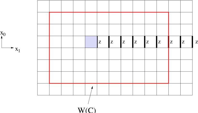
Figure 4: Creation of a center vortex (shaded plaquette) in a plane.

Since creation of a thin vortex changes plaquettes by

$$\mbox{Tr}[UUU^{\dagger}U^{\dagger}]\rightarrow z\mbox{Tr}[UUU^{\dagger}U^{\dagger}]$$ (45)

on the vortex sheet (D=4), the action of a thin vortex is singular in the continuum limit. If center vortices are found in the QCD vacuum, then we expect these to be extended objects, in which the action of of the vortex sheet is spread out into a surface of finite thickness in physical units. It is not hard to show that vortices percolating through the lattice will disorder Wilson loops, leading to an area law.

57 Direct Maximal Center Gauge

Although it is easy to describe how to create center vortices on an arbitrary background, it is not obvious how to identify such objects in any given configuration. The method which our group proposed in ref. Jan98 was to fix the lattice to a certain gauge, known as “direct maximal center gauge,” and then map the links of the gauge-fixed lattice onto center elements, a procedure known as “center projection.” An important insight into what this gauge is doing $-$ and how it can fail $-$ is due to Engelhardt and Reinhardt ER .

A typical thermalized lattice $U_{\mu}(x)$, if printed out, looks like a set of random numbers. But it is not random, and in fact locally, at $\beta\gg 1$, the link variables approximate a (classical) vacuum configuration

$$U_{\mu}(x)\approx g(x)g^{\dagger}(x+\hat{\mu})$$ (46)

Let us ask the question: What is the best fit, to a given lattice $U_{\mu}(x)$, by a pure gauge $g(x)g^{\dagger}(x+\hat{\mu})$? We work with the SU(2) gauge group for simplicity. The best fit will minimize

$$d^{2}_{F} = {1\over 4{\cal V}}\sum_{x,\mu}\mbox{Tr}\left[\left(U_{\mu}(x)-g(x)g^{\dagger}(x+\hat{\mu})\right)\times\Bigl{(}\mbox{h.c.}\Bigr{)}\right]$$ (47)

$$= {1\over 4{\cal V}}\sum_{x,\mu}2\mbox{Tr}\left[I-g^{\dagger}(x)U_{\mu}(x)g(x+\hat{\mu})\right]$$

where ${\cal V}$ is the lattice volume. Define

$${}^{g}U_{\mu}(x)=g^{\dagger}(x)U_{\mu}(x)g(x+\hat{\mu})$$ (48)

Minimizing $d_{F}^{2}$ is the same as maximizing

$$R_{L}=\sum_{x,\mu}\mbox{Tr}[{}^{g}U_{\mu}(x)]$$ (49)

which is the same as the lattice Landau gauge condition. What this demonstrates is that lattice Landau gauge is is equivalent to a best fit to a pure gauge.

Next, consider trying to make a best fit to a thin vortex configuration on a classical vacuum background

$$V_{\mu}(x)=g(x)Z_{\mu}(x)g^{\dagger}(x+\hat{\mu})$$ (50)

where $Z_{\mu}(x)=\pm 1$. This can be done in two steps. First, since the adjoint representation is blind to $Z_{\mu}$, we start by finding the best fit in the adjoint representation, minimizing

$$d^{2}_{A} = {1\over 4{\cal V}}\sum_{x,\mu}\mbox{Tr}_{A}\left[\left(U_{\mu}(x)-g(x)g^{\dagger}(x+\hat{\mu})\right)\times\Bigl{(}\mbox{h.c.}\Bigr{)}\right]$$ (51)

$$= {1\over 4{\cal V}}\sum_{x,\mu}2\mbox{Tr}_{A}\left[I-g^{\dagger}(x)U_{\mu}(x)g(x+\hat{\mu})\right]$$

which is the same as maximizing

$$R_{dmc}=\sum_{x,\mu}\mbox{Tr}_{A}[{}^{g}U_{\mu}(x)]$$ (52)

where $\mbox{Tr}_{A}$ indicates the trace in the adjoint representation. This is the direct maximal center gauge-fixing condition, which is obviously just lattice Landau gauge in the adjoint representation. Having found $g(x)$ maximizing $R_{dmc}$, we then find the $Z_{\mu}(x)$ which minimizes

$$d^{2}={1\over 4{\cal V}}\sum_{x,\mu}\mbox{Tr}\left[\left(U_{\mu}(x)-g(x)Z_{\mu}(x)g^{\dagger}(x+\hat{\mu})\right)\times\Bigl{(}\mbox{h.c.}\Bigr{)}\right]$$ (53)

in the fundamental representation. For fixed $g(x)$, this minimization is achieved by setting

$$Z_{\mu}(x)=\mbox{signTr}[{}^{g}U_{\mu}(x)]$$ (54)

This step is is known as “center projection.” It maps an SU(2) lattice to a $Z_{2}$ lattice.

The original and gauge-transformed lattices can be expressed, respectively

$$U_{\mu}(x) = g(x)Z_{\mu}(x)e^{i\delta A_{\mu}(x)}g^{\dagger}(x+\hat{\mu})$$

$${}^{g}U_{\mu}(x) = Z_{\mu}(x)e^{i\delta A_{\mu}(x)}$$ (55)

with $Z_{\mu}(x)$ the vortex background, and $\delta A_{\mu}(x)$ the fluctuation around the background. Direct maximal center gauge finds the optimal $Z_{\mu}(x)$ minimizing $\delta A_{\mu}(x)$.

Unfortunately, as also pointed out in ref. ER , there are going to be problems with this approach to vortex finding, particularly in the continuum limit. It is clear that the action density of a thin vortex is singular at “P-plaquettes”, which are plaquettes $p$ where the product of $Z_{\mu}(x)$ around the plaquette is negative, i.e. $Z(p)=-1$. P-plaquettes are dual to the thin vortex surface. Since a thermalized lattice configuration is locally close to a pure gauge at large $\beta$, i.e. $\frac{1}{2}\mbox{Tr}[U(p)]\approx 1$, it follows that the fit to a thin vortex is very bad at P-plaquette locations. As $\beta\rightarrow\infty$, the bad fit near P-plaquettes may overwhelm the good fit in the exterior region, and the best fit in the continuum limit may be no thin vortices at all.

Computer simulations tend to support this analysis. In practice it is impossible to find the global maximum of $R_{L}$ or $R_{dmc}$; instead there are various methods of finding local maxima, known as Gribov copies. Using a sophisticated gauge-fixing technique which employs simulated annealing, Bornyakov et al. BKP were able to generate Gribov copies in direct maximal center gauge with consistently higher values of $R_{dmc}$ than those achieved by previous approaches based on the over-relaxation method. However, these “better” Gribov copies had much worse center dominance properties in the scaling regime. Center dominance is the agreement between string tensions on the full and center projected lattices. Using the improved gauge fixing techniques, Bornyakov et al. found that the projected string tension is lower than the full asymptotic string tension by about 30%.

58 Direct Laplacian Center Gauge

In confronting the difficulties raised in refs. ER ; BKP , we would like to retain the strategy of finding the best fit to a vortex configuration, but avoid over-emphasizing the inevitable bad fit at P-plaquettes, which seems to be the source of those difficulties (cf. ref. Remarks ). We therefore adopt a strategy inspired in part by related work of de Forcrand et al. Alex ; Pepe , which in turn draws on the earlier Laplacian Landau gauge fixing of Vink and Weise Vink . The idea is to replace the SO(3) gauge transformation $g(x)$ in (52) by a real $3\times 3$ matrix-valued field $M(x)$, chosen to maximize

$$R_{M}=\sum_{x,\mu}\mbox{Tr}[M^{T}(x)U_{A\mu}(x)M(x+\hat{\mu})]$$ (56)

($U_{A}$ is the link in the adjoint representation) with the constraint that $M(x)$ is orthogonal “on average.”

$${1\over{\cal V}}\sum_{x}M^{T}(x)M(x)=I$$ (57)

This essentially introduces an adjustable weighting; $M(x)$ is allowed to be small where the fit to a thin vortex is bad.

$R_{M}$ is maximized (uniquely!) by finding the three lowest eigenvalues, and corresponding eigenfunctions, of the lattice Laplacian eigenvalue equation (no sum over $a=1,2,3$)

$$\sum_{y}{\cal D}_{ij}(x,y)f^{a}_{j}(y)=\lambda_{a}f^{a}_{i}(x)$$ (58)

where

$${\cal D}_{ij}(x,y)=$$ (59)

$$-\sum_{\mu}\left([U_{A\mu}(x)]_{ij}\delta_{y,x+\hat{\mu}}+[U_{A\mu}(x)]_{ji}\delta_{y,x-\hat{\mu}}\ -2\delta_{xy}\delta^{ab}\right).$$

There are standard numerical algorithms which solve this equation, and the matrix field formed by

$$M_{ab}(x)=f_{a}^{b}(x)$$ (60)

where $b=1,2,3$ denotes the three eigenvectors with lowest eigenvalues, is the matrix field maximizing $R_{M}$.

We then map $M_{ab}(x)$ to the nearest SO(3) matrix

$$[g_{A}(x)]_{ij}=\tilde{f}_{i}^{j}(x)$$ (61)

which also satisfies a Laplacian equation

$$\sum_{y}{\cal D}_{ij}(x,y)\tilde{f}^{a}_{j}(y)=\Lambda_{ac}(x)\tilde{f}^{c}_{i}(x)$$ (62)

This is equivalent to finding the SO(3)-valued matrix field closest to $M_{ab}(x)$ which is also a local maximum of $R_{dmc}$. The mapping is accomplished in two steps:

1. Polar decomposition

   $$M(x)=\pm\Omega(x)P(x)$$ (63)

   to find the SO(3) matrix $\Omega$ which is closest to $M$.

2. Relaxation $\Omega\rightarrow g_{A}$ to the nearest local maximum of

   $$R_{dmc}=\sum_{x,\mu}\mbox{Tr}[g_{A}^{T}(x)U_{A\mu}(x)g_{A}(x+\hat{\mu})]$$ (64)

Finally, transform $U_{\mu}(x)\rightarrow{}^{g}U_{\mu}(x)$. This prescription for mapping an arbitrary gauge field configuration to an (in principle unique) point on the gauge orbit is called direct Laplacian center gauge. We apply center projection

$$Z_{\mu}(x)=\mbox{signTr}[{}^{g}U_{\mu}(x)]$$ (65)

as before, to locate the P-plaquettes forming thin vortices (known as “P-vortices”) on the projected lattice.

58.1 Center Dominance

The most important property to check with the new procedure is center dominance, since this is where problems were found numerically, in refs. BKP and KT , with the previous methods.

The center vortex contribution to the asymptotic string tension is extracted from

$$W_{cp}(C)=\langle ZZ...Z\rangle$$ (66)

in the center-projected configurations, obtained after direct Laplacian gauge fixing. Creutz ratios $\chi_{cp}[R,R]$ are plotted in Fig. 5. The straight line is the asymptotic freedom behavior, with ${\sqrt{\sigma}/\Lambda}=58$

Figure 5: Projected Creutz ratios of various sizes as a function of $\beta$.

Note that the Creutz ratios at each $\beta$ are nearly the same (with the exception of the $1\times 1$ loop), and this is known as “precocious linearity.” This feature can also be clearly seen in Fig. 6. Here we also see the property of center dominance: The center-projected Creutz ratios $\chi_{cp}[R,R]$ at all $R\geq 2$ agree quite well with the full asymptotic string tension $\sigma$, extracted from unprojected Wilson loops, both at strong and weak couplings

Figure 6: Center projected Creutz ratios for various couplings and lattice sizes. Straight lines show the values of the asymptotic string tensions and corresponding error bars, in the unprojected configurations, quoted in ref. Bali .

An alternative way of displaying our data is to plot the ratio

$${\chi_{cp}[R,R]\over\sigma_{Lat}(\beta)}\equiv{\chi_{phys}[R,R]\over\sigma_{phys}}$$ (67)

as a function of $R$ in physical units, where $\sigma_{Lat}$ is the asymptotic string tension in lattice units, while the subscript “phys” refers to physical units. In Fig. 7 we see that the ratios are not far from unity (center dominance) even down to relatively small distance scales (precocious linearity).

Figure 7: Ratio of center-projected Creutz ratios $\chi[R,R]$ to the full asymptotic string tension in physical units vs. $R$ in physical units.

58.2 Other Tests

To check that P-vortices are really associated with center vortices in the full configuration, and are not just artifacts of the projection, it is necessary to verify their correlation with gauge invariant observables. Such tests were invented in refs. Us ; Jan98 and dFE , and it is important to repeat these with the new method. Here I will only touch on the results.

We define the “vortex-limited” Wilson loops $W_{n}(C)$ to be loops evaluated on a subensemble of configurations, selected such that precisely  $n$  P-vortices, in the corresponding center-projection, pierce the loop. Center projection is used only to select the data set. The loops themselves are evaluated using the full, unprojected link variables. What we find numerically is that in the limit of large loops,

$${W_{n}(C)\over W_{0}(C)}~{}~{}\longrightarrow~{}~{}(-1)^{n}$$ (68)

This is what one expects, if P-vortices locate thick center vortices in the unprojected SU(2) lattice.

It is also possible to measure the density of P-vortices as a function of $\beta$. If $N_{vor}$ is the number of P-vortex plaquettes, and $N_{T}$ is the total number of plaquettes on the lattice, then the density of P-vortices in lattice units is given by

$$p = {N_{vor}\over N_{T}}={N_{vor}a^{2}\over N_{T}a^{4}}a^{2}$$ (69)

$$= {\mbox{Total Vortex Area}\over 6\times\mbox{Total Volume}}a^{2}={1\over 6}\rho a^{2}$$

where $\rho$ is the center vortex density (area per unit volume) in physical units. According to asymptotic freedom, if the P-vortices are locating physical objects, we should have

$$p={\rho\over 6\Lambda^{2}}\left({6\pi^{2}\over 11}\beta\right)^{102/121}\exp\left[-{6\pi^{2}\over 11}\beta\right]$$ (70)

But also $p$ is related to the center-projected one-plaquette loop

$$W_{cp}(1,1)=(1-p)\times(+1)+p\times(-1)=1-2p$$ (71)

which allows us to calculate $p$ from center-projected plaquette values. It is found that the the data for $p$ is quite consistent with the asymptotic freedom result (70).

Finally, as suggested by de Forcrand and D’Elia dFE , one can remove center vortices from the gauge-fixed configuration by simply multiplying by the projected configuration

$${}^{g}U_{\mu}(x)\rightarrow{}^{g}U^{\prime}_{\mu}(x)=Z_{\mu}(x){}^{g}U_{\mu}(x)$$ (72)

What we find, using the direct Laplacian gauge procedure, is that confinement disappears when vortices are removed in this way.

59 Conclusions

The conclusion we draw from all this is that center vortices in the Yang-Mills vacuum are correctly located by the new procedure, and these vortices are responsible for the confining force. Direct Laplacian center gauge combined with center projection is found to be an improvement over the original approach to locating center vortices in lattice configurations, and presumably works well even in the continuum limit. It should be a useful tool for the further study of the center vortex “spaghetti vacuum;” a picture of the QCD vacuum very similar to that proposed by Holger Nielsen and Poul Olesen back in 1978.

References

- (1) P. Becher and H. Joos (1982), The Dirac-Kähler equation and Fermions on the Lattice., Z. Phys. C-Part. and Fields 15, 343-365.
- (2) Anamarija Borštnik and Norma Susana Mankoč Borštnik (1999). Are Spins and Charges Unified? How Can One Otherwise Understand Connection Between Handedness (Spin) and Weak Charge? Proceedings to the International Workshop on ”What Comes Beyond the Standard Model, Bled, Slovenia, 29 June-9 July 1998 Ed. by N. Mankoč Borštnik, H. B. Nielsen, C. Froggatt, DMFA Založništvo 1999, p. 52-57, hep-ph/9905357, and the paper in preparation.
- (3) Howard Georgi (1982). Lie Algebra in Particle Physics, The Benjamin/Cummings Publishing Company, Inc. Advanced Book Program.
- (4) Hitochi Ikemori (1987). Superfield Formulation of Relativistic Superparticle , Phys.Lett. 199, 239-242.
- (5) Erich Kähler (1962), Der innere Differentialkalkül, Rend. Mat. Ser.V, 21, 452-523.
- (6) Norma Susana Mankoč Borštnik (1992). Spin Connection as a Superpartner of a Vielbein, Phys. Lett. B 292 25-29. From a World-sheet Supersymmetry to the Dirac Equation Nuovo Cimento A 105, 1461-1471.
- (7) Norma Susana Mankoč Borštnik (1993). Spinor and Vector Representations in Four Dimensional Grassmann Space J. Math. Phys. 34 3731-3745.
- (8) Norma Susana Mankoč Borštnik (1994). Spinors, Vectors and Scalars in Grassmann Space and Canonical Quantization for Fermions and Bosons, Int. Jour. Mod. Phys. A 9 1731-1745; Unification of Spins and Charges in Grassmann Space hep-th/9408002; Qantum Mechanics in Grassmann Space, Supersymmetry and Gravity hep-th/9406083.
- (9) Norma Susana Mankoč Borštnik (1995). Poincaré Algebra in Ordinary and Grassmann Space and Supersymmetry J. Math. Phys. 36, 1593-1601; Unification of Spins and Charges in Grassmann Space Mod. Phys. Lett. A 10, 587-595; hep-th/9512050
- (10) Norma Susana Mankoč Borštnik (1999,2001). Unification of Spins and Charges in Grassmann Space, hep-ph/9905357, In. J. of Theor. Phys. 40 315-337 Proceedings to the International Workshop ”What Comes Beyond the Standard Model”, Bled, Slovenia, 29 June-9 July 1998, Ed. by N. Mankoč Borštnik, H. B. Nielsen, C. Froggatt, DMFA Založništvo 1999, p. 20-29.
- (11) Norma Susana Mankoč Borštnik and Svjetlana Fajfer (1997), Spins and Charges, the Algebra and Subalgebras of the Group SO(1,14), Nuovo Cimento B 112 , 1637-1665; hep-th/9506175.
- (12) Norma Susana Mankoč Borštnik and Holger Bech Nielsen (1999). Dirac-Káhler Approach Conencted to Quantum Mechanics in Grassmann Space, to appear in Phys. Rev. D15; hep-th/9911032, Proceedings to the International Workshop ”What Comes Beyond the Standard Model”, Bled, Slovenia, 29 June - 9 July 1998, Ed. by N. Mankoč Borštnik, H. B. Nielsen, C. Froggatt, DMFA Založništvo 1999, p. 68-73; hep-ph/9905357; hep-th/9909169.
- (13) Holger Bech Nielsen and M. Ninomija (1981). A No-go Theorem for Regularizing Chiral Fermions Phys. Lett. B 105, 219-223; Nucl. Phys. B 185, Absence of Neutrinos on a Lattice, 20-40.
- (14) Julius Wess and Jonathan Bagger (1983). Supersymmetry and Supergravity, Princeton Series in Physics, Princeton University Press, Princeton, New Jersey.
- (15) Norma Susana Mankoč Borštnik and Holger Bech Nielsen (2002). Coupling constant unification in spin-charge unifying model agreeing with proton decay measurement, in preparation.
- (16) Anamarija Borštnik and Norma Susana Mankoč Borštnik and Holger Bech Nielsen (2002). Where do families of left handed weak charge doublets and right handed weak charge singlets come from?, in preparation.

References

- (1) Z.Koba and H.B.Nielsen, Nucl.Phys.B10,633(1969)
- (2) Z.Koba and H.B.Nielsen, Nucl.Phys.B12,517(1969)
- (3) Z.Koba and H.B.Nielsen, Z.Physik 229,243(1969)
-
(4)
Y.Nambu, Proceedings of the International Conference on
Symmetries and Quark Models,edited by R.Chand.Gordan and Breach
(1970) p.269;
H.B.Nielsen, in High Energy Physics, Proceedings of the 15th International Conference on High Energy Physics,
Kiev 1970, edited by V.Shelest(Naukova,Dunika,Kiev,
USSR, 1972);
L.Susskind, Phys.Rev.Letts.23, 545 (1969) - (5) P.H.Frampton in ”Dual Resonance Models”,(Frontiers in Physics, no.5), W.A.Benjamin, Inc (1974).
- (6) H.B.Nielsen and P.Olesen, Nucl.Phys.B61,45(1973)
-
(7)
M.Axenides, E.G.Floratos, S.Komineas and L.Perivolaro
poulos, ”Metastable Ringlike Semitopological Solitons”, Phys.Rev.Letts 86, 4459 (2001) - (8) T.D. Lee and Y. Pang, Phys. Rept. 221 (1992) 251
- (9) S. Coleman, Nucl. Phys. B262 (1985) 263
- (10) R. Battye and P. Sutcliffe, Nucl. Phys. B590, 329 (2000) [hep-th/0003252].
- (11) S. Komineas and L. Perivolaropoulos,http://leandros.chem.demokritos.gr/qballs, http://leandros.chem.demokritos.gr/qballs/3Dplots.html
- (12) E. Witten, Nucl. Phys. B249, 557 (1985).
- (13) D. Haws, M. Hindmarsh and N. Turok, Phys. Lett. B209, 255 (1988).
- (14) G.H. Derrick, J. Math Phys. 5, 1252 (1964)
- (15) A. Kusenko, Phys. Lett. B404 (1997) 285, hep-th/9704073
- (16) M. Axenides, S. Komineas, L. Perivolaropoulos and E. Floratos, Phys. Rev. D61, 085006 (2000) [hep-ph/9910388].
- (17) L. Faddeev and A. J. Niemi, Nature 387, 58 (1997) [hep-th/9610193].
-
(18)
L. Perivolaropoulos, “Superconducting semilocal stringy (Hopf)
textures,” in ESF Network Workshop Les Houches, France,
1999 hep-ph/9903539
L. Perivolaropoulos and T. N. Tomaras, Phys. Rev. D62, 025012 (2000) [hep-ph/9911227]. - (19) S. Kasuya and M. Kawasaki, “Q-ball formation through Affleck-Dine mechanism,”hep-ph/9909509.

References

- (1) S. Adler, Phys. Rev. 177, 2426 (1969); J. S. Bell and R. Jackiw, Nuovo Cimento, 60A, 47 (1969); R. A. Bertlmann, ’Anomalies in quantum field theory’, Oxford, UK: Clarendon (1996) and references therein.
- (2) D. Melikhov and B. Stech, hep-ph/0108165.
- (3) A. D. Dolgov and V. I. Zakharov, Nucl. Phys. B27, 525 (1971); V. I. Zakharov, Phys. Rev. D42, 1208 (1990).
- (4) D. Melikhov, Phys. Lett. B380, 363 (1996).
- (5) I. V. Musatov and A.V. Radyushkin, Phys. Rev. D 56, 2713 (1997).
- (6) P. Ball and V. M. Braun, Phys. Rev. D 58, 094016 (1999).
- (7) M. Beyer, D. Melikhov, N. Nikitin, and B. Stech, Phys. Rev. D64, 094006 (2001).

References

-
(1)
M. Maltoni, V.A. Novikov, L.B. Okun, A.N. Rozanov, M.I. Vysotsky: Extra quark-lepton generations and precision measurements,
Phys. Lett. B476, (2000), 107–115.
M. Maltoni: Ph.D. thesis, hep-ph/0002143, Ch. 5, (2000). - (2) V.A. Novikov, L.B. Okun, A.N. Rozanov, M.I. Vysotsky: Extra generations and discrepancies of electroweak precision data, hep-ph/0111028.
- (3) J.F. Gunion, D. McKay, H. Pois: A Minimal Four-Family Supergravity Model, Phys. Rev. D53, (1996), 1616–1647.
-
(4)
H. B. Nielsen, A. V. Novikov, V. A. Novikov, M. I. Vysotsky: Higgs potential bounds on extra quark-lepton generations, Phys. Lett.
B374, (1996), 127–130.
Yu. F. Pirogov, O.V. Zenin: Two-loop renormalization group restrictions on the standard model and the fourth chiral family, Eur. Phys. J. C10, (1999), 629–638. - (5) L3 Coll: Search for Charginos with a Small Mass Difference to the Lightest Supersymmetric Particle at , Phys. Lett. B482, (2000), 31–42.
- (6) OPAL Coll., G. Abbieudi et al: Search for Unstable Heavy and Excited Leptons at LEP2, Eur. Phys. J. C14, (2000), 73–84.
- (7) W. S. Hou, R. Stuart: Higgs-boson production from decays of the fourth-generation quark, Phys. Rev. D43, (1991), 3669–3682.
- (8) CDF Coll., T. Affolder et al: Search for a Fourth-Generation Quark More Massive than the Boson in Collisions at , Phys. Rev. Lett. 84, (2000), 835–840.
- (9) S. P. Martin: A Supersymmetry Primer, hep-ph/9709356.
- (10) C.-H. Chen, M. Drees, J. F. Gunion: A Non-Standard String/SUSY Scenario and its Phenomenological Implications, Phys. Rev. D55, (1997), 330–347.
- (11) DELPHI Coll., P. Abreu et al: A Search for Heavy Stable and Long-Lived Squarks and Sleptons in Collisions at Energies from 130 to 183 GeV, Phys. Lett. B444, (1998), 491–502.
- (12) D. E. Groom et al: Particle Data Group Coll., Eur. Phys. J. C15, (2000), 1.
- (13) W. de Boer, G. Burkart, R. Ehret, W. Oberschulte-Beckmann, V. Bednyakov, S. G. Kovalenko: Combined Fit of Low Energy Constraints to Minimal Supersymmetry and Discovery Potential at LEPII, hep-ph/9507291.
- (14) D. M. Ghilencea, G. G. Ross: Precision prediction of gauge couplings and the profile of a string theory, Nucl. Phys. B606, (2001), 101.
- (15) P. Langacker, N. Polonsky: Uncertainties in Coupling Constant Unification, Phys. Rev. D47, (1993), 4028 - 4045.
- (16) ALEPH, DELPHI, L3 and OPAL Coll: Searches for Invisible Higgs bosons: Preliminary combined results using LEP data collected at energies up to , hep-ex/0107032.

References

- (1) Fairlie D.B., Govaerts J. and Morozov A., Universal Field Equations with Covariant Solutions, Nuclear Physics B 373 (1992) 214-232.
-
(2)
Baker L.M. and Fairlie D.B., Companion Equations for Branes, (1999) , Journal of Mathematical Physics 41 (2000) 4284-4292.
Baker L.M. and Fairlie D.B., Hamilton-Jacobi equations and Brane associated Lagrangians, Nuclear Physics B596 (2001) 348-364. - (3) Fairlie D.B The Multi-field Complex Bateman Equation, hep-th 0106003 to appear in Letters in Math. Phys (2001).
- (4) Chaundy T. , The Differential Calculus Oxford University Press (1935) p. 328.
-
(5)
Fairlie D.B. and Leznov A.N.,
The Complex Bateman Equation, Letters in Math. Physics 49(1999) 213-216.
Fairlie D.B. and Leznov A.N., The Complex Bateman equation in a space of arbitrary dimensions, Journal of Mathematical Physics 42 (2001) 453-462. - (6) Fairlie D.B. and Mulvey J.A., Integrable Generalisations of the 2-dimensional Born Infeld Equation, J. Phys A27 (1994) 1317-1324.
- (7) Arik M., Neyzi F., Nutku Y., Olver P.J. and Verosky J., Multi-Hamiltonian structure of the Born Infeld equations, J.Math. Phys 30 (1989) 1338-1344.
- (8) Fairlie D.B., Integrable Systems in Higher Dimensions Quantum Field Theory, Integrable Models and Beyond Editors. T. Inami and R. Sasaki Progress of Theoretical Physics Supplement 118 (1995) 309-327.
- (9) Fairlie D.B.,Dirac-Born-Infeld Equations, Phys .Lett. B456, (1999) 141-146.
- (10) Leznov A.N., Journal of Nonlinear Mathematical Physics 8:(1) (2001)1-7;also ’Integrable Hierarchies and Modern Physical Theories NATO Science Series ed. Henrik Aratun and A.Sorin,‘ Mathematics, Physics and Chemistry-V0l. 18 (2001)

References

- (1) An introduction to nonassociative algebras, Richard D. Schafer. New York, Academic Press, 1966.
- (2) P. Jordan, Z. Phys. 80, 285 (1933).
- (3) P. Jordan, J. Von Neumann and E.P. Wigner, Ann. Math. 35, 29 (1934).
- (4) A.A. Albert, Ann. Math. 35, 65 (1934).
- (5) M. Gunaydin and F. Gursey, J. Math. Phys. 14, 1651 (1973).
- (6) Nonassociative algebra and its applications : the fourth international conference / edited by R. Costa … [et al.]. New York : Marcel Dekker, c2000.
- (7) Nonassociative algebras in physics / J. Lhmus, E. Paal, and L. Sorgsepp, Palm Harbor, FL : Hadronic Press, 1994.
- (8) B. Grossman, T. W. Kephart and J. D. Stasheff, Commun. Math. Phys. 96, 431 (1984) [Erratum-ibid. 100, 311 (1984)].
- (9) S. Fubini and H. Nicolai, Phys. Lett. B 155, 369 (1985).
- (10) M. J. Duff and J. X. Lu, Phys. Rev. Lett. 66, 1402 (1991).
- (11) J. A. Harvey and A. Strominger, Phys. Rev. Lett. 66, 549 (1991).
- (12) A survey of binary systems, R. H. Bruck, in Ergebnisse der Mathematik und ihrer Grenzgebiete Berlin, Heft 20, Springer, 1958.
- (13) ”Latin squares and their applications,” J. Dénes and A. D. Keedwell. London : English Universities Press, 1974.
- (14) ”Discrete mathematics using Latin squares,”Charles F. Laywine and Gary L. Mullen, New York : Wiley, 1998.
- (15) Orthogonal arrays : theory and applications, A.S. Heydayat, N.J.A. Sloane, J. Stufken. Springer series in statistics, Springer, New York, 1999.
- (16) Projektive Ebenen, Pickert, G. Die Grundlagen der mathematischen Wissenschaften in Einzeldarstellungen Bd. 80, Berlin, Springer, 1955.
- (17) Nonassociative Tangles, by D. Bar-Natan in Geometric topology : 1993 Georgia International Topology Conference, University of Georgia, Athens, Georgia / William H. Kazez, editor. Providence, R.I. : American Mathematical Society : International Press, 1997

References

- (1) H. Goldstein, Classical Mechanics (Addison-Wesley, 1950)
- (2) L.D. Landau and E.M. Lifshitz, Fluid Mechanics (Pergamon Press, 1959)
- (3) R.P. Feynman, in: Progr. in Low Temp. Phys., ed. C.J. Gorter (North Holland; Amsterdam, 1955), Vol.I, ch.2
-
(4)
P.A.M. Dirac, Proc. Roy. Soc. A33 (1931) 60
G. ’t Hooft, Nucl. Phys. B79 (1974) 276
A.M. Polyakov, JETP Lett. 20 (1974) 194 -
(5)
F. London, in Superfluids (J. Wiley & Sons,
N.Y. 1950) 152
A.A. Abrikosov, Sov. Phys. JETP 5 (1957), 1174
H.B. Nielsen and P. Olesen, Nucl. Phys. B61 (1973) 45

References

- (1) J.L. Petersen, J. Rasmussen and M. Yu, Nucl. Phys. B 457 (1995) 309
- (2) J.L. Petersen, J. Rasmussen and M. Yu, Nucl. Phys. B 457 (1995) 343
- (3) J.L. Petersen, J. Rasmussen and M. Yu, in Proceedings of the workshop Gauge Theories, Applied Supersymmetry and Quantum Gravity, Leuven July 1995, Leuven Notes in Mathematical and Theoretical Physics, Vol. 6, Eds. B. de Wit et al (Leuven 1996) hep-th/9510059
- (4) J.L. Petersen, J. Rasmussen and M. Yu, Nucl. Phys. B (Proc. Suppl.) 49 (1996) 27
- (5) J.L. Petersen, J. Rasmussen and M. Yu, Nucl. Phys. B 481 (1996) 577
- (6) J.L. Petersen, J. Rasmussen and M. Yu, in Proceedings of Inauguration Conference of the Asia Pacific Center for Theoretical Physics (APCTP), Seoul, Korea, 1996
- (7) J.L. Petersen, J. Rasmussen and M. Yu, Nucl. Phys. B 502 (1997) 649
- (8) J. Rasmussen, hep-th/9610167, Ph.D. thesis (The Niels Bohr Institute)
- (9) V.G. Kac and D.A. Kazhdan, Adv. Math. 34 (1979) 97
- (10) F.G. Malikov, B.L. Feigin and D.B. Fuks, Funkt. Anal. Prilozhen 20 (1986) 25
- (11) D. Bernard and G. Felder, Commun. Math. Phys. 127 (1990) 145
- (12) H. Awata, A. Tsuchiya and Y. Yamada, Nucl. Phys. B 365 (1991) 680; H. Awata, Prog. Theor. Phys. Suppl. 110 (1992) 303
-
(13)
P. Furlan, A.Ch. Ganchev, R. Paunov and V.B. Petkova,
Phys. Lett. B 267 (1991) 63;
P. Furlan, A.Ch. Ganchev, R. Paunov and V.B. Petkova, Nucl. Phys. B 394 (1993) 665;
A.Ch. Ganchev and V.B. Petkova, Phys. Lett. B 293 (1992) 56 -
(14)
Vl.S. Dotsenko, Nucl. Phys. B 338 (1990) 747;
Vl.S. Dotsenko, Nucl. Phys. B 358 (1991) 547 - (15) K. Amoto, J. Math. Soc. Japan 39 (1987) 191
- (16) V.V. Schechtman and A.N. Varchenko, Invent. Math. 106 (1991) 139
-
(17)
B. Feigin and F. Malikov, Adv. Sov. Math. 17 (1993) 15,
hep-th/9306137;
K. Iohara and F. Malikov, Mod. Phys. Lett. A 8 (1993) 3613 -
(18)
G. Felder and A. Varchenko, hep-th/9502165, preprint;
G. Felder and C. Wieczerkowski, hep-th/9411004, preprint -
(19)
B.L. Feigin and E.V. Frenkel, Usp. Mat. Nauk. 43 (1988) 227
(in Russian), Russ. Math. Surv. 43 (1989) 221;
B.L. Feigin and E.V. Frenkel, Commun. Math. Phys. 128 (1990) 161;
B.L. Feigin and E.V. Frenkel, Lett. Math. Phys. 19 (1990) 307;
B.L. Feigin and E.V. Frenkel, in Physics and Mathematics of Strings, Eds. L. Brink et al. (World Scientific, 1990);
E. Frenkel, Free field realizations in representation theory and conformal field theory, preprint hep-th/9408109 -
(20)
O. Andreev, Int. J. Mod. Phys. A 10 (1995) 3221;
O. Andreev, Phys. Lett. B 363 (1995) 166 - (21) H. Awata and Y. Yamada, Mod. Phys. Lett. A7 (1992) 1185
- (22) B. Feigin and F. Malikov, Lett. Math. Phys 31 (1994) 315
- (23) B. Feigin and F. Malikov, preprint q-alg/9511011
- (24) M. Wakimoto, Commun. Math. Phys. 104 (1986) 60
- (25) M. Bershadsky and H. Ooguri, Commun. Math. Phys. 126 (1989) 49
- (26) V. Knizhnik and A. Zamolodchikov, Nucl. Phys. B 247 (1984) 83
- (27) P. Christe and R. Flume, Nucl. Phys. B 282 (1987) 466
- (28) V.A. Fateev and A.B. Zamolodchikov, Sov. J. Nucl. Phys. 43 (1986) 657
-
(29)
Vl.S. Dotsenko and V.A. Fateev, Nucl. Phys. B 240[FS12] (1984) 312;
Vl.S. Dotsenko and V.A. Fateev, Nucl. Phys. B 251[FS13] (1985) 691 -
(30)
A.C. McBride and G.F. Roach (eds.) Fractional Calculus
(Pitman Advanced Publishing Program) (Boston 1985);
S.G. Samko, A.A. Kilbas and O.L. Marichec, Fractional Integrals and Derivatives, Gordon and Breach, Science Publishers (1993) -
(31)
A. Morozov, JETP Lett. 49 (1989) 345;
A. Gerasimov, A. Marshakov, A. Morozov, M. Olshanetskii, and S. Shatashvili, Int. J. Mod. Phys. A 5 (1990) 2495 -
(32)
P. Bouwknegt, J. McCarthy and K. Pilch, Phys. Lett. B 234 (1990) 297;
P. Bouwknegt, J. McCarthy and K. Pilch, Commun. Math. Phys. 131 (1990) 125;
P. Bouwknegt, J. McCarthy and K. Pilch, Prog. Theor. Phys. Suppl. 102 (1990) 67;
P. Bouwknegt, J. McCarthy and K. Pilch in Strings and symmetries 1991, eds. N. Berkovits et al., (World Scientific, Singapore, 1992) -
(33)
M. Kuwahara and H. Suzuki, Phys. Lett. B 235 (1990) 52;
M. Kuwahara, N. Ohta and H. Suzuki, Phys. Lett. B 235 (1990) 57;
M. Kuwahara, N. Ohta and H. Suzuki, Nucl. Phys. B 340 (1990) 448;
N. Ohta and H. Suzuki, Nucl. Phys. B 332 (1990) 146 - (34) K. Ito, Phys. Lett. B 252 (1990) 69
-
(35)
K. Ito and Y. Kazama, Mod. Phys. Lett. A 5 (1990) 215;
K. Ito and S. Komata, Mod. Phys. Lett. A 6 (1991) 581 - (36) G. Kuroki, Commun. Math. Phys. 142 (1991) 511
- (37) W. Taylor IV, LBL-34507, hep-th/9310040, Ph.D. thesis
-
(38)
J. de Boer and L. Fehér, Mod. Phys. Lett. A 11 (1996)
1999;
J. de Boer and L. Fehér, Wakimoto realizations of current algebras: an explicit construction, LBNL-39562, UCB-PTH-96/49, BONN-TH-96/16, hep-th/9611083, preprint -
(39)
V.G. Kac and M. Wakimoto, Proc. Natl. Acad. Sci.
USA 85 (1988) 4956;
V.G. Kac, and D.A. Kazhdan, Adv. Ser. Math. Phys., Vol. 7 (World Scientific, 1989), p. 138

References

-
(1)
H.B.Nielsen, ”Dual Strings. Fundamental of Quark Models”, in:
Proceedings of the XYII Scottish University Summer School in Physics, St.Andrews, 1976, p.528. -
(2)
H.B.Nielsen, D.L.Bennett, N.Brene, Recent Developments in Quantum
Field Theory, Amsterdam, 1985, p.263;
D.L.Bennett, H.B.Nielsen, I.Picek, Phys.Lett. B208, 275 (1988). - (3) H.B.Nielsen, Acta Physica Polonica, B20, 427 (1989).
- (4) H.B.Nielsen, N.Brene, Phys.Lett. B233, 399 (1989); Phys. Mag. 12, 157 (1989); Nucl.Phys. B359, 406 (1991).
- (5) C.D.Froggatt, H.B.Nielsen, Origin of Symmetries, Singapore: World Scientific, 1991.
-
(6)
L.Nottalle, Int.J.Mod.Phys. A7, 4899 (1992);
L.Nottale, Fractal Space-Time and Microphysics, Singapore: World Scientific, 1993;
L.Nottalle and J.Schneider, J.Math.Phys. 25, 1296 (1984). - (7) H.P.Nilles, Phys.Reports 110, 1 (1984).
- (8) P.Langacker, N.Polonsky, Phys.Rev. D47, 4028 (1993); ibid, D49, 1454 (1994); ibid, D52, 3081 (1995).
- (9) D.L.Bennett and H.B.Nielsen, Int.J.Mod.Phys. A9, 5155 (1994); ibid, A14, 3313 (1999).
- (10) L.V.Laperashvili, Phys. of Atom.Nucl. 57, 471 (1994); ibid, 59, 162 (1996).
- (11) L.V.Laperashvili and H.B.Nielsen, Mod.Phys.Lett. A12, 73 (1997).
- (12) L.V.Laperashvili and H.B.Nielsen, ”Multiple Point Principle and Phase Transition in Gauge Theories”, in: Proceedings of the International Workshop on ”What Comes Beyond the Standard Model”, Bled, Slovenia, 29 June - 9 July 1998; Ljubljana 1999, p.15.
- (13) L.V.Laperashvili and H.B.Nielsen, Int.J.Mod.Phys. A16, 2365 (2001).
-
(14)
L.V.Laperashvili, H.B.Nielsen and D.A.Ryzhikh,
Int.J.Mod.Phys. A16, 3989 (2001);
L.V.Laperashvili, H.B.Nielsen and D.A.Ryzhikh, Yad.Fiz. 65 (2002). -
(15)
C.D.Froggatt, G.Lowe, H.B.Nielsen, Phys.Lett. B311, 163 (1993);
Nucl.Phys. B414, 579 (1994); ibid B420, 3 (1994);
C.D.Froggatt, H.B.Nielsen, D.J.Smith, Phys.Lett. B358, 150 (1996);
C.D.Froggatt, M.Gibson, H.B.Nielsen, D.J.Smith, Int.J.Mod.Phys. A13, 5037 (1998);
H.B.Nielsen, C.D.Froggatt, ”Masses and Mixing Angles and Going beyond the Standard Model”, in Proceedings of the International Workshop on ”What Comes Beyond the Standard Model?”, Bled, Slovenia, 29 June - 9 July 1998: Ljubljana 1999, p.29. - (16) C.D.Froggatt, L.V.Laperashvili, H.B.Nielsen, ”SUSY or NOT SUSY”, ”SUSY98”, Oxford, 10-17 July 1998; hepnts1.rl.ac.uk/susy98/.
- (17) H.B.Nielsen, Y.Takanishi, Nucl.Phys. B588, 281 (2000); ibid, B604, 405 (2001); Phys.Lett. B507, 241 (2001); hep-ph/0011168, hep-ph/0101181, hep-ph/0101307.
- (18) L.V.Laperashvili, ”Anti–Grand Unification and Phase Transitions at the Planck Scale in Gauge Theories”, in: ”Frontiers of Fundamental Physics”, Proceedings of Forth International Symposium, Hyderabad, India, 11-13 December, 2000. Ed. B.G.Sidharth.
- (19) K.Wilson, Phys.Rev. D10, 2445 (1974).
-
(20)
J.Jersak, T.Neuhaus and P.M.Zerwas, Phys.Lett. B133, 103 (1983);
Nucl.Phys. B251, 299 (1985);
H.G.Everetz, T.Jersak, T.Neuhaus, P.M.Zerwas, Nucl.Phys. B251, 279 (1985). -
(21)
G.Parisi, R.Petronzio, F.Rapuano, Phys.Lett. B128, 418 (1983);
E.Marinari, M.Guagnelli, M.P.Lombardo, G.Parisi, G.Salina, Proceedings Lattice ’91’, Tsukuba 1991, p.278-280; Nucl.Phys.Proc.Suppl. B26, 278 (1992). - (22) G.Bhanot, Nucl.Phys. B205, 168 (1982); Phys.Rev. D24, 461 (1981); Nucl.Phys. B378, 633 (1992).
-
(23)
M.Lüscher, K.Symanzik, P.Weisz, Nucl.Phys. B173, 365 (1980);
C.Surlykke, On Monopole Suppression in Lattice QED, preprint NBI (1994). -
(24)
T.Suzuki, Progr.Theor.Phys. 80, 929 (1988);
S.Maedan, T.Suzuki, Progr.Theor.Phys. 81, 229 (1989). -
(25)
S.Coleman and E.Weinberg, Phys.Rev. D7, 1888 (1973);
S.Coleman, in: Laws of Hadronic Matter, edited by A.Zichichi, Academic Press, New York, 1975. - (26) M.Sher, Phys.Rept. 179, 274 (1989).
- (27) G. ’t Hooft, Nucl.Phys. B190, 455 (1981).
- (28) M.B.Voloshin and K.A.Ter-Martirosyan, Theory of Gauge Interactions of Elementary Particles, Energoatomizdat, 1984.
- (29) P.A.Kovalenko, L.V.Laperashvili, Phys. of Atom.Nucl. 62, 1729 (1999).
- (30) S.Rajpoot, Nucl.Phys.Proc.Suppl. 51A, 50 (1996).
-
(31)
D.Zwanziger, Phys.Rev. D3, 343 (1971);
R.A.Brandt, F.Neri, D.Zwanziger, Phys.Rev.D19, 1153 (1979). - (32) F.V.Gubarev, M.I.Polikarpov, V.I.Zakharov, Phys.Lett.B438, 147 (1998).
- (33) L.V.Laperashvili, H.B.Nielsen, Mod.Phys.Lett. A14, 2797 (1999).

References

- (1) J. Hoppe, Ph. D. thesis, MIT (1982); J. Hoppe, Int. J. Mod. Phys. A4(1989)5235.
- (2) E. G. Floratos, J. Iliopoulos, and G. Tiktopoulos, Phys. Lett. B217(1989)285.
- (3) D. Fairlie, P. Fletcher, and G. Zachos, Phys. Lett. B218(1989)203; D. Fairlie and G. Zachos, Phys. Lett. B224(1989)101; D. Fairlie, P. Fletcher, and G. Zachos, J. Mat. Phys. 31(1990)1088.
- (4) I. Bars, Phys. Lett. B245(1990)35.
- (5) W. Krauth and M. Staudacher, Phys. Lett. B435(1998)350.
- (6) J. Hotta, J. Nishimura and A. Tsuchiya, Nucl. Phys. B545(1999)543
- (7) P. Austing and J. F. Wheater, hep-th/0101071.
- (8) K. N. Anagnostopoulos, J. Nishimura, and P. Olesen, hep-th/0012061.
- (9) O. Alvarez, Phys. Rev. D24(1981)440.
- (10) P. Olesen, Phys. Lett. B160(1985)144.

References

- (1) Ziro Koba, Holger Bech Nielsen, MANIFESTLY CROSSING INVARIANT PARAMETRIZATION OF N MESON AMPLITUDE. Nucl.Phys.B12:517-536,1969
- (2) A. Kraemmer, H. Nielsen, and L. Susskind, Nucl. Phys. B28, 34 (1971);
- (3) M. Karliner, I. Klebanov and L Susskind, Size And Shape Of Strings Int.J.Mod.Phys. A3 (1988) 1981
- (4) G. ’t Hooft A Planar Diagram Theory For Strong Interactions, Nucl.Phys. B72 (1974) 461
- (5) Holger Bech Nielsen, P. Olesen, VORTEX LINE MODELS FOR DUAL STRINGS, Nucl.Phys.B61:45-61,1973
- (6) Joseph Polchinski, Matthew J. Strassler, The String Dual of a Confining Four-Dimensional Gauge Theory, hep-th/0003136
- (7) Joseph Polchinski , Matthew J. Strassler HARD SCATTERING AND GAUGE / STRING DUALITY. hep-th/0109174
- (8) R.R. Metsaev, C.B. Thorn, A.A. Tseytlin, Light-cone Superstring in AdS Space-time, hep-th/0009171

References

- (1) I. Shapiro, Phys. Rev. Lett. 13, 789 (1964); see also S. Weinberg, Gravitation and Cosmology, Wiley, 1972.
- (2) L.B. Okun, Mod. Phys. Lett. A15, 1941 (2000).
- (3) L.D. Landau and E.M. Lifshits, Teoriya Polya, Moscow, Nauka, 1967 (in Russian); Classical Field Theory, Pergamon Press 1961 (in English).
- (4) C.W. Misner, K.S. Thorne, J.A. Wheeler, Gravitation, W. H. Freeman & Co., 1971.
- (5) A.P. Lightman, W.H. Press, R.H. Price, S.A. Teukolsky, Problem Book in Relativity and Gravitation, Princeton U., 1975.
- (6) L.D. Landau and E.M. Lifshits, Hydrodynamics (in Russian), Moscow, Nauka, 1986.
- (7) L.D. Landau and E.M. Lifshits, Fluid Mechanics, Oxford, Pergamon Press 1982.
- (8) R. Kubo, Statistical Mechanics, North-Holland 1965.
- (9) F.R. Tangherlini, Schwarzschild field in n-dimensions and the dimensionality of space problem, Nuovo Cimento, 27, 636 (1963).
- (10) R.C. Myers and M.J. Perry, “Black holes in higher dimensional spaces”, Ann. Phys. 172, 304 (1986);

References

- (1) H. B. Nielsen and P. Olesen, Nucl. Phys. B160 (1979) 380
- (2) G. ’t Hooft, Nucl. Phys. B138 (1978) 1; G. Mack, in Recent Developments in Gauge Theories, edited by G. ’t Hooft et al. (Plenum, New York, 1980).
- (3) L. Del Debbio, M. Faber, J. Greensite, and Š. Olejník, Phys. Rev. D55 (1997) 2298, hep-lat/9610005.
- (4) L. Del Debbio, M. Faber, J. Giedt, J. Greensite, and Š. Olejník, Phys. Rev. D58 (1998) 094501, hep-lat/9801027.
- (5) M. Engelhardt and H. Reinhardt, Nucl. Phys. B567 (2000) 249, hep-th/9907139.
- (6) V. Bornyakov, D. Komarov, and M. Polikarpov, Phys. Lett. B497 (2001) 151, hep-lat/0009035.
- (7) M. Faber, J. Greensite, and Š. Olejník, hep-lat/0103030.
- (8) C. Alexandrou, M. D’Elia, and Ph. de Forcrand, Nucl. Phys. Proc. Suppl. 83 (2000) 437, hep-lat/9907028.
- (9) Ph. de Forcrand and M. Pepe, Nucl. Phys. B598 (2001) 557, hep-lat/0008016.
- (10) J. Vink and U. Weise, Phys. Lett. B289 (1992) 122, hep-lat/9206006.
- (11) T. Kovacs and E. Tomboulis, Phys. Lett. B463 (1999) 104.
-
(12)
C. Michael and M. Teper, Phys. Lett. B199 (1987) 95;
G. Bali, C. Schlichter, and K. Schilling, Phys. Rev. D51 (1995) 5165, hep-lat/9409005. - (13) Ph. de Forcrand and M. D’Elia, Phys. Rev. Lett. 82 (1999) 4582, hep-lat/9901020.
Blejske Delavnice Iz Fizike, Letnik 2, št. 2, ISSN 1580–4992
Bled Workshops in Physics, Vol. 2, No. 2
Zbornik delavnic ‘What comes beyond the Standard model’, 2000 in 2001
Zvezek 1: Zbornik ob 60. rojstnem dnevu Holgerja Bech Nielsena
Proceedings to the workshops ‘What comes beyond the Standard model’, 2000 and 2001
Volume 1: Festschrift dedicated to the 60th birthday of Holger Bech Nielsen
Uredili in oblikovali Norma Mankoč Borštnik, Colin D. Froggat in Dragan Lukman
Publikacijo sofinancira Ministrstvo za šolstvo, znanost in šport
Tehnični urednik Vladimir Bensa
Založilo: DMFA – založništvo, Jadranska 19, 1000 Ljubljana, Slovenija
Natisnila Tiskarna MIGRAF v nakladi 100 izvodov
Publikacija DMFA številka 1479