Abstract

A new method to construct event-generators based on next-to-leading order QCD matrix-elements and leading-logarithmic parton showers is proposed. Matrix elements of loop diagram as well as those of a tree level can be generated using an automatic system. A soft/collinear singularity is treated using a leading-log subtraction method. Higher order re-summation of the soft/collinear correction by the parton shower method is combined with the NLO matrix-element without any double-counting in this method.

An example of the event generator for Drell-Yan process is given for demonstrating a validity of this method.

1 Introduction

The standard model(SM) of electromagnetic and strong interactions has been well established through precision measurements of a large variety of observables in high-energy experiments[1]. However, there is still one missing part of the SM to be confirmed by experiments, i.e. the Higgs boson. In order to search for this missing part and also search for direct signals beyond the SM, the LHC experiments[2] are under construction at CERN. Though LHC has employed a proton-proton colliding machine due to their high discovery potential for new (heavy) particles, a capability for precision measurements must also be seriously considered. For extracting physically meaningful information from a large amount of experimental data, suffered from huge QCD backgrounds, a deep understanding of the behavior of QCD backgrounds is essentially important.

The prediction power of a lowest calculation of QCD processes is very limited due to a large coupling constant of the strong interaction and an ambiguity of the renormalization energy scale. Predictions based on the NLO (or more) matrix elements combined with some all-order summation are desirable. Much effort to calculate NNLO corrections[3] is being made for LHC experiments. Moreover, in order to suit for precision measurements, a simple correction factor (so-called $K$-factor) for the lowest calculation is clearly not sufficient. One must construct event generators including NLO matrix elements with higher order re-summation even for processes with multi-particle final states. When one tries to do this task, one may encounter the following difficulties:

• the number of diagram contributing to processes with many particles in a final state is very large,

• many parton-level processes must be combined to construct a proton-(anti-)proton collision,

• numerical instability in the treatment of a collinear singularity may appear,

• a careful treatment of matching between matrix elements and the re-summation part must be required to avoid double counting, and

• negative weight of events in some part of phase space is not avoidable.

In order to overcome these difficulties, lots of works have already been done[3, 4]. In this report, we propose a new method to construct event-generators with next-to-leading order QCD matrix-elements and leading-logarithmic parton showers. Our solution for the above problems will be given in this report.

2 Matrix elements

A calculation of the matrix elements of hard-scattering processes is not a simple task when multiple partons are produced. At the tree level, the GRACE system[5], an automatic system for generating Feynman diagram and a FORTRAN source-code to evaluate the amplitude, is established. The system can in principle treat any number of external particles, and has been used for up to six fermions[6] in the final state within a practical CPU time. In the GRACE system, matrix elements are calculated numerically using a CHANEL[7] library based on a helicity amplitude. CHANEL contains routines to evaluate such things as: wave-functions/spinors at external states, interaction vertices, and particle propagator.

Based on this method, we have already published an event generator of four $b$-quark generation processes at proton-(anti-)proton collisions at tree-level named GR@PPA_4b[8], which include all possible tree-level diagram to create four $b$-quarks in final state with an interface to PYTHIA[9].

For the loop diagram, effective vertices of two- and three-point functions have been prepared[10] and implemented in the system. At first amplitudes of the loop diagram are evaluated in $d$-dimensional space-time. The dimensionless coupling constant is introduced as $g\rightarrow{\tilde{\mu}}^{d/2-2}g$. After the loop-momentum integration, $UV$ divergences are eliminated by subtracting $1/\varepsilon_{UV}+\gamma_{E}-\ln 4\pi$ where $\varepsilon_{UV}=2-d/2$ and $\gamma_{E}$ is the Euler’s constant. This is so-called $\overline{MS}$ renormalization scheme[11]. Then we are left with the infra-red divergence which is also regularized using the dimensional regularization by setting $d=4+2\varepsilon_{IR}$, where $\varepsilon_{IR}>0$.

Expressions of effective vertices after the $\overline{MS}$ renormalization are summarized in Appendix A. For more than three-point diagram, an extended CHANEL is prepared. It can evaluate a fermion current including any number of gamma matrices. An amplitude of loop diagram will be calculated based on the fermion current connected by boson propagators. When a fermion loop is included in the diagram, numerical calculation will be performed after taking its trace. A bosonic loop can also be treated by the CHANEL.

3 Loop integral

As two- and three-point functions are embedded in the system as effective vertices, loop integrals which must be done in each process start from four-point functions. The loop-momentum integration of the four-point diagram can be expressed as

$$I_{4}(p_{1},p_{2},p_{3},p_{4}) = \left(\mu^{2}\right)^{\varepsilon_{UV}}\int\frac{d^{d}k}{(2\pi)^{d}i}\frac{1}{A_{1}A_{2}A_{3}A_{4}},$$ (1)

$$A_{1} = k^{2}+i0,$$

$$A_{2} = (k+p_{1})^{2}+i0,$$

$$A_{3} = (k+p_{1}+p_{2})^{2}+i0,$$

$$A_{4} = (k+p_{1}+p_{2}+p_{3})^{2}+i0,$$

$$p_{1}+p_{2}+p_{3}+p_{4} = 0,$$

where $k$ is a loop momentum and $p_{i}$’s are external momentum taken to be incoming. After a momentum integration using an usual procedure of Feynman-parameter method, the integral can be represented as

$$I_{4}(p_{1},p_{2},p_{3},p_{4}) = \frac{\Gamma(2-\varepsilon_{IR})}{(4\pi)^{2}}{\tilde{J}}_{4}(s,t,m_{1}^{2},m_{2}^{2},m_{3}^{2},m_{4}^{2}),$$ (2)

where $m_{i}^{2}=p_{i}^{2}$, $s=(p_{1}+p_{2})^{2}$, and $t=(p_{1}+p_{4})^{2}$. In general we need tensor integrals

$$J_{4}(s,t;n_{x},n_{y},n_{z})=$$ (3)

$$\left(4\pi\mu^{2}\right)^{-\varepsilon_{IR}}\int_{0}^{1}dx~{}dy~{}dz\frac{x^{n_{x}}y^{n_{y}}z^{n_{z}}}{\left(-xzs-y(1-x-y-z)t-i0\right)^{2-\varepsilon_{IR}}},$$

here we set all external particles on-shell (massless). A method to perform this integration is well established. The scaler integrations (when $n_{x}=n_{y}=n_{z}=0$) without an infrared divergence are given in [12] and those with IR divergence are given in [13]. Tensor integrals can be obtained from a linear combination of scaler integrals [14]. Even though the method is well established, we decided to develop our own method for the tensor integration of an IR divergent case, in order to avoid a possible numerical instability due to some cancellation among IR divergent scaler integrals.

The tensor integration can be done analytically and be represented by a finite number of terms with Beta and Hypergeometric functions as;

$$J_{4}(s,t;n_{x},n_{y},n_{z})=\frac{1}{s~{}t}\frac{B(n_{x}+\varepsilon_{IR},n_{y}+n_{z}+\varepsilon_{IR})}{1-\varepsilon_{IR}}$$ (4)

$$\times \biggl{[}\left(\frac{-{\tilde{t}}}{4\pi\mu^{2}}\right)^{\varepsilon_{IR}}\left(\frac{-t}{s}\right)^{n_{x}}\frac{n_{x}}{\prod_{j=1}^{n_{x}}({n_{x}}-j+\varepsilon_{IR})}B(1+n_{z},n_{x}+n_{y}+\varepsilon_{IR})$$

$$\times {{}_{2}F_{1}}\left(1+n_{x},n_{x}+n_{z}+\varepsilon_{IR},1+n_{x}+n_{y}+n_{z}+\varepsilon_{IR},-\frac{{\tilde{u}}}{{\tilde{s}}}\right)$$

$$+ \left(\frac{-{\tilde{s}}}{4\pi\mu^{2}}\right)^{\varepsilon_{IR}}\sum_{l=0}^{n_{x}}\left(\frac{-s}{t}\right)^{l}\frac{\prod_{j=1}^{l}(l-j-n_{x})}{\prod_{j=1}^{l}(l-j+\varepsilon_{IR})}B(1+n_{y},l+n_{z}+\varepsilon_{IR})$$

$$\times {{}_{2}F_{1}}\left(1+l,l+n_{z}+\varepsilon_{IR},1+l+n_{y}+n_{z}+\varepsilon_{IR},-\frac{{\tilde{u}}}{\bar{t}}\right)\biggr{]},$$

$${{\tilde{s}}} = s+i0,$$

$${{\tilde{t}}} = t+i0,$$

$${\bar{t}} = t-i0,$$

$${{\tilde{u}}} = u+i0=(p_{1}+p_{3})^{2}+i0.$$

When the numerator is unity ($n_{x}=n_{y}=n_{z}=0$), the scalar integration can be obtained as

$$J_{4}(s,t;0,0,0)=\frac{1}{s~{}t}\frac{B(\varepsilon_{IR},\varepsilon_{IR})}{\varepsilon_{IR}(1-\varepsilon_{IR})}$$ (5)

$$\times \left[\left(\frac{-{\tilde{s}}}{4\pi\mu^{2}}\right)^{\varepsilon_{IR}}{{}_{2}F_{1}}\left(1,\varepsilon_{IR},1+\varepsilon_{IR},-\frac{{\tilde{u}}}{\bar{t}}\right)+\left(\frac{-{\tilde{t}}}{4\pi\mu^{2}}\right)^{\varepsilon_{IR}}{{}_{2}F_{1}}\left(1,\varepsilon_{IR},1+\varepsilon_{IR},-\frac{{\tilde{u}}}{{\tilde{s}}}\right)\right]$$

A explicit structure of the infra-red singularity can be obtained with Laurent expansion of above formula with respect to $\varepsilon_{IR}$. A full set of formulae and a computer program for the numerical calculation can be found in [16]

For more than four-point functions, a reduction formula[15] is used in the system.

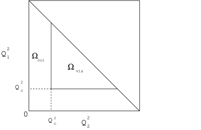
Figure 1: Dalitz plot of (N+1)-body phase space. $Q^{2}_{i}$ is defined in Eq.(6) and $Q^{2}_{c}$ is a threshold value to separate the visible- and collinear-region.

4 Real emission

4.1 Soft/Collinear treatment

At first, the conventional method of phase-space slicing[17] is used to treat soft and collinear singularities. It is explained for the case of an initial-state radiation in this report. The final-state radiation can be treated in a similar way. Let’s consider two colored partons, whose momenta are $p^{\mu}_{1}$ and $p^{\mu}_{2}$, scattered into the $N$-body final state of colorless particles as a Born process. For the radiative correction of this process, we must treat processes with one additional colored parton, whose momentum is $k^{\mu}$, emitted in addition to the Born process. The matrix elements of the real emission processes must be integrated in ($N$+1)-body phase-space, $\Phi^{(d)}_{N+1}$, in a $d$-dimensional space-time. The space-time dimension is set to be $d=4+2\varepsilon_{IR}$ in this report. A collinear region in the ($N+1$)-body phase-space of the final particles in the $d$-dimensional space-time is defined as

$$\Omega_{coll} = \Phi^{(d)}_{N+1}\wedge\{k^{\mu}|Q^{2}_{i}=-(p_{i}-k)^{2}<Q^{2}_{c}\}\subset\Omega_{full}=\Phi^{(d)}_{N+1},$$ (6)

as shown in figure 1, where $Q^{2}_{c}$ is some cut-off value. It must be sufficiently small so as not to be observed experimentally. Final results must be independent of this value. In the collinear region, matrix elements can be approximated as

$$\biggl{|}{\cal M}^{(d)}_{N+1}\biggr{|}^{2} = \biggl{|}{\cal M}^{(4)}_{N}\biggl{(}q\rightarrow\sum_{i=1}^{N}q_{i}\biggr{)}\biggr{|}^{2}\frac{16\pi}{s\mu^{2\varepsilon_{IR}}}f_{c}\frac{\alpha_{s}}{2\pi}{\tt P}(x)\frac{1}{k_{T}^{2}}\biggl{(}\frac{1-x}{x}\biggr{)},$$ (7)

$$q^{\mu} = p_{1}^{\mu}+p_{2}^{\mu}-k^{\mu},$$

where ${\tt P}(x)$ is a splitting function for a given parton splitting at a leading-logarithmic order, $k_{T}$ is the transverse momentum of the radiated parton, $f_{c}$ is a color factor of a given branching and $\mu$ the energy scale of the splitting. The CM-energy of the Born process is ${\hat{s}}=q^{2}=sx$, where $s=(p_{1}+p_{2})^{2}$. Here, we can set $d$ to be four in the matrix element of the Born process, since it has no IR singularity. In the same approximation, the phase space is expressed as

$$d\Phi^{(d)}_{N+1} = d\Phi^{(4)}_{N}\biggl{(}q\rightarrow\sum_{i=1}^{N}q_{i}\biggr{)}$$ (8)

$$\times \frac{1}{16\pi^{2}\Gamma(1+\varepsilon_{IR})}\biggl{(}\frac{k_{T}^{2}}{4\pi x^{2}}\biggr{)}^{\varepsilon_{IR}}\frac{1}{1-x}dxdk_{T}^{2}.$$

The total cross section of real-radiation processes in the collinear region can be obtained as

$$\sigma_{coll} = \frac{1}{(2p^{0}_{1})(2p^{0}_{2})v_{rel}}\int_{\Omega_{coll}}d\Phi^{(d)}_{N+1}\biggl{|}{\cal M}^{(d)}_{N+1}\biggr{|}^{2},$$ (9)

$$= \frac{1}{(2p^{0}_{1})(2p^{0}_{2})v_{rel}}\biggl{[}\int_{\Omega_{full}}d\Phi^{(d)}_{N+1}-\int_{\Omega_{vis}}d\Phi^{(d)}_{N+1}\biggr{]}\biggl{|}{\cal M}^{(d)}_{N+1}\biggr{|}^{2},$$ (10)

where $\Omega_{vis}$ means a visible region of the phase space, such as

$$\Omega_{vis} = \Omega_{full}-\Omega_{coll}.$$ (11)

Then, the collinear cross section can be obtained after the integration with respect to $k^{2}_{T}$ as

$$\sigma_{coll} = \sigma_{full}-\sigma_{vis},$$ (12)

$$\sigma_{full} = \frac{1}{(2p^{0}_{1})(2p^{0}_{2})v_{rel}}\int_{\Omega_{full}}d\Phi^{(d)}_{N+1}\biggl{|}{\cal M}^{(d)}_{N+1}\biggr{|}^{2},$$ (13)

$$= \left(\frac{s}{4\pi\mu^{2}}\right)^{\varepsilon_{IR}}\frac{B(\varepsilon_{IR},\varepsilon_{IR})}{2\Gamma(1+\varepsilon_{IR})}f_{c}\frac{\alpha_{s}}{2\pi}\int_{0}^{1}dx\sigma_{0}(xs){\tt P}(x)\left(\frac{1-x}{x}\right)^{2\varepsilon_{IR}},$$ (14)

$$\sigma_{vis} = \frac{1}{(2p^{0}_{1})(2p^{0}_{2})v_{rel}}\int_{\Omega_{vis}}d\Phi^{(d)}_{N+1}\biggl{|}{\cal M}^{(d)}_{N+1}\biggr{|}^{2},$$ (15)

$$= 2f_{c}\frac{\alpha_{s}}{2\pi}\int_{0}^{1}dx\sigma_{0}(xs){\tt P}(x)\ln{\biggl{(}\frac{s}{Q_{c}^{2}}(1-x)-1\biggr{)}}\Theta\biggl{(}1-\frac{2Q_{c}^{2}}{s}-x\biggr{)},$$ (16)

where

$$\sigma_{0}(xs) = \frac{1}{x(2p^{0}_{1})(2p^{0}_{2})v_{rel}}\int d\Phi^{(4)}_{N}\biggl{|}{\cal M}^{(4)}_{N}\biggl{(}q\rightarrow\sum_{i=1}^{N}q_{i}\biggr{)}\biggr{|}^{2}_{q^{2}=xs},$$ (17)

is the Born cross-section at a CM energy of $q^{2}=xs$ in four-dimensional space-time, $\mu$ is a factorization energy scale, and $\Theta$ is a step function. For example in case of a splitting for a quark to quark+gluon, $\sigma_{coll}$ after the $\varepsilon_{IR}$ expansion becomes

$$\sigma_{coll} = \sigma_{0}(s)\frac{\alpha_{s}}{2\pi}f_{c}\biggl{[}\frac{2}{\varepsilon_{IR}^{2}}+\frac{2L-3}{\varepsilon_{IR}}-\frac{\pi^{2}}{2}+L^{2}\biggr{]}$$ (18)

$$+ 2\int_{0}^{1}dx\sigma_{0}(xs)\phi(x,\varepsilon_{IR})$$

$$+ 2f_{c}\frac{\alpha_{s}}{2\pi}\int_{0}^{1}dx\sigma_{0}(xs)\left[L\frac{1+x^{2}}{(1-x)_{+}}+2\frac{(1+x^{2})\ln{(1-x)}}{(1-x)_{+}}-\frac{1+x^{2}}{1-x}\ln{x}\right]$$

$$- 2f_{c}\frac{\alpha_{s}}{2\pi}\int_{0}^{1}dx\sigma_{0}(xs)\frac{1+x^{2}}{(1-x)_{+}}\ln{\biggl{(}\frac{s}{Q_{c}^{2}}(1-x)-1\biggr{)}}\Theta\biggl{(}1-\frac{2Q_{c}^{2}}{s}-x\biggr{)},$$

where

$$\phi(x,\varepsilon_{IR}) = \frac{1}{\varepsilon_{IR}}f_{c}\frac{\alpha_{s}}{2\pi}{\tt P}(x)=\frac{1}{\varepsilon_{IR}}f_{c}\frac{\alpha_{s}}{2\pi}\frac{1+x^{2}}{(1-x)_{+}},$$ (19)

$$L = \ln{(s/\mu^{2})}.$$ (20)

The IR-divergent terms in the collinear cross section can be canceled out after summing up terms from virtual corrections. After combining with virtual corrections, there still exists the collinear-divergent term, $\phi(x,\varepsilon_{IR})$. This term is thrown away by hand, because it is counted in the PDF or PS on the initial partons. Since the $\overline{MS}$ renormalization scheme is used in this calculation, the same scheme must be used in the PDF or PS.

4.2 Visible jet cross-section

The last part of the NLO cross-section calculation is a real emission of the additional parton into the visible region with exact matrix elements. Those matrix elements of ($N$+1)-parton production at the final state in four-dimensional space-time can be automatically generated using the GRACE system. Cross sections are obtained by integrating those matrix elements under the four-dimensional phase-space as

$$\sigma_{exact} = \frac{1}{(2p^{0}_{1})(2p^{0}_{2})v_{rel}}\int_{\Omega_{vis}}d\Phi^{(4)}_{N+1}\biggl{|}{\cal M}^{(4)}_{N+1}\biggr{|}^{2}.$$ (21)

The space-time dimension is set to be four ($\varepsilon_{IR}=0$) hereafter, since there is no IR-divergence in $\Omega_{vis}$. When the threshold energy ($Q_{c}^{2}$) is set to be sufficiently small, this cross section can be larger than the Born cross section due to the large magnitude of the coupling constant ($\alpha_{s}$). A parton-level calculation has no problem, except for the large higher-order correction. However, if one tries to calculate the cross sections of a proton (anti-)proton collision, one has to combine the matrix elements with the PDF or PS to construct a proton from partons. The PDF and PS include leading-log(LL) terms of the initial-state parton emission. If the matrix element is combined with the PDF or PS very naively, a double-counting of these LL-terms must be unavoidable. Our proposal to solve this problem is to subtract the LL-terms from the exact matrix elements as

$$\sigma_{LLsub} = \frac{1}{(2p^{0}_{1})(2p^{0}_{2})v_{rel}}\int_{\Omega_{vis}}d\Phi^{(4)}_{N+1}\biggl{[}\biggl{|}{\cal M}^{(4)}_{N+1}\biggr{|}^{2}-\biggl{|}{\cal M}^{(4)}_{N}(sx)\biggr{|}^{2}f_{LL}(x,s)\biggr{]},$$ (22)

$$f_{LL}(x,s) = f_{c}\frac{\alpha_{s}}{2\pi}{\tt P}(x)\frac{16\pi^{2}}{k_{T}^{2}}\biggl{(}\frac{1-x}{x}\biggr{)}.$$ (23)

The second term of the integrand is the LL-approximation of the real-emission matrix-elements under the collinear condition. There is nothing but ’$\sigma_{vis}$’ in the last subsection. Then the real-emission cross section ($\sigma_{real}$) can be expressed as

$$\sigma_{real} = \sigma_{col}+\sigma_{exact},$$ (24)

$$= \sigma_{full}-\sigma_{vis}+\sigma_{exact},$$ (25)

$$= \sigma_{full}+\sigma_{LLsub}.$$ (26)

One can expect a numerically stable calculation using Eq.(26) rather than Eq.(24), because cancellation between $\sigma_{vis}$ and $\sigma_{exact}$ occurred before the phase-space integration. When the threshold value of $Q^{2}_{c}$ is set to be sufficiently small, the integrand in $\sigma_{LLsub}$ is very close to zero, because the LL-approximation is very precise around the collinear region. Then, the result of integration in $\sigma_{LLsub}$ is independent of the threshold value of $Q_{c}^{2}$.

This subtraction may distort the experimental observables of additional jet distributions. However, a subtracted LL-part will be recovered after adding the PS applied in the Born process. The exact matrix element of real-radiation processes gives only non-logarithmic terms to the visible distributions in the LL-subtraction method. The relation between the PS and the LL-subtraction method is as follows. The LL-approximation cross section in $\sigma_{LLsub}$ is

$$\sigma_{LL} = \frac{1}{(2p^{0}_{1})(2p^{0}_{2})v_{rel}}\int_{\Omega_{vis}}d\Phi^{(4)}_{N+1}\biggl{|}{\cal M}^{(4)}_{N}(sx)\biggr{|}^{2}f_{LL}(x,s)$$ (27)

$$= \int_{0}^{1}dx\sigma_{0}(xs){\cal D}^{\small(1)}(x),$$ (28)

$${\cal D}^{\small(1)}(x) = \int_{Q_{c}^{2}/(1-x)}^{Q_{max}^{2}}\frac{dk_{T}^{2}}{k_{T}^{2}}f_{c}\frac{\alpha_{s}}{2\pi}{\tt P}(x),$$ (29)

where $Q_{max}^{2}$ is the maximum value of the transverse momentum. ${\cal D}^{\small(1)}(x)$ is just the first term of the all-order re-summation of the leading logarithmic terms in the PS. Actually, some special case of the Sudakov form factor can be obtained from ${\cal D}^{\small(1)}(x)$as:

$$\Pi(Q^{2}_{max},Q^{2}_{c}/(1-x)) = exp\biggl{(}-\int^{1}_{0}{\cal D}^{\small(1)}(x)dx\biggr{)}.$$ (30)

However, there is one essential difference between ${\cal D}^{\small(1)}(x)$ and the Sudakov form factor in the PS: the upper bound of $k_{T}^{2}$ integration. In the PS, this integration is performed up to the energy scale determined by the Born process instead of their maximum value in kinetically allowed region. Then, if $\sigma_{LL}$ is subtracted in the full phase space of the ($N$+1)-particle final state, some part of the LL cross section cannot be recovered from the Born cross-section with the PS. Then, an appropriate restriction on the phase-space integration must be applied, such as

$${\tilde{\sigma}}_{LLsub} = \frac{1}{(2p^{0}_{1})(2p^{0}_{2})v_{rel}}\int_{\Omega_{vis}}d\Phi^{(4)}_{N+1}\biggl{[}\biggl{|}{\cal M}^{(4)}_{N+1}\biggr{|}^{2}-\biggl{|}{\cal M}^{(4)}_{N}(sx)\biggr{|}^{2}f_{LL}(x,s)\Theta(Q_{B}^{2}-k_{T}^{2})\biggr{]},$$ (31)

where $Q_{B}^{2}$ is the energy scale of the Born process, which must be the same as the factorization energy-scale of the PS.

Figure 2: Momentum fraction distributions from an x-deterministic parton shower and Cteq5L parton distribution functions. The distributions of $u$-quarks (left), ${\bar{u}}$-quarks (center), and gluons (right) are shown.

5 Event generation with a parton shower

5.1 Conventional method

The calculations of cross sections for proton-(anti) proton collisions are usually performed as follows[9, 18]:

1. matrix elements of a given process at a parton level are prepared,

2. a probability to observe a parton in a proton at given energy scale and momentum fraction is obtained from some parton distribution function(PDF)[19],

3. a numerical integration is performed in phase-space with some initial energy distribution in the PDF,

4. for initial-state partons, a (backward) parton shower[20] is applied from the given (high) energy scale to a low energy-scale of partons,

5. for final-state partons, a parton shower is also applied from a given energy scale to close to the hadron energy-scale,

6. some non-perturbative effects according to string fragmentation or color clustering are taken into account, and

7. physical hadrons are formed based on some hadronization model.

In this method, the parton shower(PS) is used in a supplementary way, just for generating multi-partons with a finite transverse momentum.

5.2 An $x$-deterministic PS

The parton shower is a method to solve a DGLAP evolution equation[21] using a Monte Carlo method. The PDF’s are also obtained by solving the DGLAP equation with experimental data-fitting. When an initial distribution of partons is given at some energy scale, the PS can reproduce a consistent result as the PDF. For singlet partons, we employ an evolution scheme based on momentum distributions rather than those on particle-number distributions, which is used for non-singlet processes. The momentum-distribution evolution-scheme has been proposed by Tanaka and Munehisa[22] and shows numerically stable results with high efficiency.

The PDF can give the weight of partons when the momentum fraction ($x$) and the energy scale are given by the users. On the other hand, in the forward evolution scheme of the PS, the momentum fraction of a parton ($x$) is determined only after evolution takes place. This method is very inefficient, for instance, for a narrow-resonance production. In order to cure this inefficiency, we have developed an $x$-deterministic PS. In a Monte-Carlo procedure in the PS, the $Q^{2}$ evolution is controlled by the Sudakov form-factor, which gives a non-branching probability of partons, and the $x$ determination is done independently according to a splitting function. It is not necessary to determine the $x$ value at each branching. After preforming all branching procedures using the Sudakov form-factor, the $x$ value at each branching is determined to give a total $x$, being a given value from outside of the PS. In this PS, each event has a different weight according to the splitting functions and initial distribution of the PDF. When the number of branchings is $n$, the weight of this event ($W$) can be obtained as

$$W = \frac{1}{W_{0}}\prod_{i=1}^{n}P(x_{i})F_{\small PDF}(x_{0})dx_{i}dx_{0},$$ (32)

$$W_{0} = \prod_{j=1}^{n}\int_{0}^{1}P(x_{j})dx_{j},$$ (33)

where $P(x_{i})$ is a splitting function, $F_{\small PDF}(x_{0})$ is parton distribution function, and $x_{0}$ is a momentum fraction before the parton-shower evolution. The momentum fraction after the evolution is $x=\prod_{i=0}^{n}x_{i}$. In order to take this momentum fraction ($x$) as an independent variable given by users, unity

$$1=\int\delta(x-{\small x_{0}\prod_{j=1}^{n}x_{j}})dx$$ (34)

is multiplied to Eq.(32) and integration by $dx_{0}$ is done first as

$$W = \frac{1}{W_{0}}\prod_{i=1}^{n}P(x_{i})F_{\small PDF}(x_{0})\delta\biggl{(}x-{\small x_{0}\prod_{j=1}^{n}x_{j}}\biggr{)}dxdx_{i}dx_{0},$$ (35)

$$= \frac{1}{W_{0}}\prod_{i=1}^{n}P(x_{i})F_{\small PDF}({\tilde{x}_{0}})\frac{dx_{i}dx}{\prod_{j=1}^{n}x_{j}},$$ (36)

$${\tilde{x}_{0}} = \frac{x}{\prod_{j=1}^{n}x_{j}}.$$ (37)

If we employ an appropriate transformation of the input random numbers, we can expect a sufficient efficiency.

A numerical test of the $x$-deterministic PS is done by comparing results with the PDF of Cteq5L[23]. The initial distributions of partons are taken from Cteq5L at the energy scale of the $b$-quark mass. Then, after evolution to an energy scale of 100 GeV, the $x$ distributions from the PS are compared to those in Cteq5L. One can see in Fig.2 the PS reproduced $x$ distributions in Cteq5L for both of singlet and non-singlet partons.

Our procedure to generate QCD events involves the following three steps, :

1. numerical integration is performed in the phase-space including $x$ integration,

2. the probability for the existence of each parton in the proton at some low-energy scale is obtained from the PDF, and

3. the $x$-deterministic PS performs evolution from a low energy scale to the energy scale of a hard scattering while generating multi-partons with a finite transverse momentum,

instead of steps 2, 3, and 4 in the conventional procedure.

5.3 Negative weight treatment

Though the LL-subtraction method makes the negative-positive cancellation in the collinear region very mild, the NLO amplitude may still have negative values in some region in the phase-space. This negative weight is unavoidable due to the perturbative calculation truncated at a finite order of expansion. Especially this problem is very serious in QCD due to its large expansion coefficient. Even if there are events with negative weight, experimentally measurable distributions can be positive with a realistic detector resolution (or a bin-width of histograms). Then we decided to employ a ’quasi-unweighted’ event generation as follows.

The BASES[24] system can treat integrand with negative values and prepare a table of a probability density according to the absolute value of the integrand. The SPRING[24, 25] will generate events based on that table with unit-weight with sign $+1$ or $-1$ according to a sign of integrand at given phase point. This sign will be kept during detector simulations and user analysis programs. Finally some bins of histograms will be incremented or decremented by unit amount due to their sign.

Figure 3: Transverse momentum distribution of gluons. The distributions from the PS applied to the Born process are shown by $*$ commonly in three histograms. Those distributions from $\sigma_{exact}$ (left), $\sigma_{exact}$ with double-count rejection (middle), and $\sigma_{exact}$ with double-count rejection and the $k_{T}^{2}$ restriction are compared with the PS.

6 A test of the LL-subtraction method

The LL-subtraction method is numerically tested for a process of $u{\bar{u}}\rightarrow\mu^{+}\mu^{-}$ in proton-anti proton collision at the CM energy of 2 TeV. Here only non-singlet $u$-quark is used in this test to avoid additional complex problem. Matrix elements of the Born process and the real radiation process ($u{\bar{u}}\rightarrow\mu^{+}\mu^{-}gluon$) are generated by GRACE. Numerical integration is done using a BASES system. A non-singlet $u$-quark distribution at the energy scale of 4.6 GeV is taken from CTEQ5L. The parton evolution from this energy scale to that of hard-scattering, i.e. an invariant mass of the muon-pair (${\hat{s}}_{\mu\mu}$), is done using the $x$-deterministic PS for both of the Born and radiative processes. An additional cut of $\sqrt{{\hat{s}}_{\mu\mu}}>40$ GeV is also applied.

The distributions of transverse momenta of gluons are shown in Figure 2. For the Born process, the largest $k_{T}$ from the PS is filled to histograms if it has $k_{T}$ greater than 1 GeV. For the radiative process, that from matrix elements is filled when it has passed the same cut as mentioned above. If one does not take care of double-counting of the LL-terms in the matrix elements and the PS, the distributions of $d\sigma_{exact}/dk_{T}$ show larger values compared with the PS in the Born process, as shown in the left histogram of Figure 2. In order to avoid double-counting, we required that $k_{T}$ of the matrix elements be greater than those of any gluons from the PS in the radiative process. This double-counting rejection leads to a good agreement of the $k_{T}$ distribution around the low-$k_{T}$ region, as shown in the middle histogram. However, the PS still emits an insufficient number of gluons around a very high-$k_{T}$ region. If the upper bound of the $k_{T}^{2}$ integration is set to be ${\hat{s}}_{\mu\mu}$ in the calculation with the exact matrix elements, $k_{T}^{2}$ distributions shows a good agreement, as shown in right histogram. This behavior tells us that the parton-shower can reproduce gluon distributions only for the energy scale less than ${\hat{s}}_{\mu\mu}$. This result confirmed the necessity of the step function ($\Theta(Q^{2}_{B}-k_{T})$) in Eq.(31).

The distributions from ${\tilde{\sigma}}_{LLsub}$ combined with those of the PS on the Born process are compared with those from exact matrix-elements with double-counting rejection. In both of the gluon energy and the transverse-momentum distributions, the LL-subtraction method can give consistent results with those of the exact matrix elements, as shown in Figure 3.

Figure 4: Energy and transverse momentum distributions of gluons. The $*$ shows the distributions from the PS on the Born process, solid histograms from $\sigma_{exact}$ with double-count rejection, and circles from ${\tilde{\sigma}}_{LLsub}$ combined with those from the PS on the Born process.

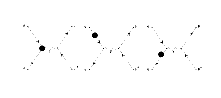
Figure 5: Feynman diagram of the Drell-Yan process, $q{\bar{q}}\rightarrow{\mu}^{-}{\mu}^{+}$ and its radiative processes.

.

Figure 6: Transverse energy distributions ($E_{T}$) of jets (left figure) and muon-pair system (right figure). For a jet distribution, the largest $E_{T}$ among jets from parton showers or matrix elements are filled in the histogram. Solid histograms show distributions from parton showers applied on the tree+virtual+collinear collections, dashed ones come from real radiation matrix-elements with PS+(LL-subtraction), and dot-dashed ones come from the matrix-elements with PDF without any care of the double-counting.

.

7 Example:Drell-Yan processes

In order to demonstrate how our proposed method can really work for physical processes in hadron colliders, an example of an event generator for the Drell-Yan process in a proton anti-proton ($p{\bar{p}}$) collider of TEVATRON at the next-to-leading order QCD is constructed. All possible Feynman diagram contributing to the process $p{\bar{p}}\rightarrow\mu^{+}\mu^{-}$(+additional parton) as shown in figure 5 are taken into account in the generator. All quarks and gluons except top-quark in an initial (anti-)proton are summed up using the PDF of Cteq5L at $b$-quark mass of 4.5 GeV and $Q^{2}$ evolution to the energy scale of a hard scattering has been done using the $x$-deterministic parton shower at leading logarithmic order.

FORTRAN programs to calculate matrix-elements are automatically generated using GRACE including loop- and real-radiation diagram as well as tree ones. All quark masses are set to be massless in the matrix-element calculations. A QCD coupling constant is calculated using a leading-order formula with $\Lambda_{QCD}=146$ MeV which is obtained by parameter fittings in Cteq5L. The factorization scale is set to be equal to the energy of a $\mu$-pair system. As it is known well for the Drell-Yan process, the renormalization energy scale does not explicitly appear in the correction terms. Main correction terms are absorbed in the running coupling constant and $Q^{2}$ evolution of the parton distribution. Remaining terms with the large logarithm ($L=\ln(Q^{2}/\mu)Z$) is canceled out after summing up virtual and collinear correction terms. This renormalization scale independence is numerically checked in our program. Infrared divergent part proportional to $1/\varepsilon_{IR}^{2}$ and $1/\varepsilon_{IR}$ are left in the program and numerically confirmed that these divergent coefficients are canceled out after summing up virtual and collinear parts of the matrix elements at the order of $10^{-20}$. No experimental cut except the energy of a $\mu$-pair system to be greater than 10 GeV is applied. The total cross section of the Drell-Yan process at 2 TeV of the $p{\bar{p}}$ CM energy with above cut is obtained to be $1.026\times 10^{3}$ pb at the tree level and $1.288\times 10^{3}$ pb at the NLO, which gives a $K$-factor of 1.256. In the cross section of $1.288\times 10^{3}$ pb at the NLO, $1.807\times 10^{2}$ pb comes from the visible cross section after the LL-subtraction. It is rather good behavior as perturbative correction of QCD. Numerical results of the virtual and collinear correction of $q{\bar{q}}$ initial state are compared with those based on formulae given by Altarelli et al.[26] and are confirmed consistent. It is confirmed that the cross sections are independent from the value of $Q^{2}_{c}$ defined in section 4.2 and agree with those with simple phase-space slicing method as expected.

Next let us look at transverse energy distributions of the largest $E_{T}$ jet and a $\mu$-pair system. Origin of the transverse energy has two sources, one is finite transverse momentum of the PS and the other is that from real-radiation matrix-elements. In the LL-subtraction method, these two kinds of distributions can be smoothly combined without any double-counting. As shown in figure 6, contribution from the parton shower applied on the NLO matrix elements (solid histograms) is dominated around small $E_{T}$ region. On the other hand a high $E_{T}$ events are dominated by the real-radiation correction (dashed histograms). These two regions are smoothly connected as shown by stars (*) which show the sum of solid and dashed histograms. If one applied PDF simply on the the real-radiation matrix-elements without any care of double counting, small $E_{T}$ events are clearly over estimated as shown by dot-dashed histograms. On the other hand, high $E_{T}$ events are consistent with those from LL-subtraction method, because they are free from both double-counting and smearing due to the PS.

8 Conclusions

A new method to construct event-generators based on next-to-leading order QCD matrix-elements and an $x$-deterministic parton shower is proposed. Matrix elements of loop diagram as well as those of a tree level can be generated by the GRACE system. A soft/collinear singularity is treated using the leading-log subtraction method. It has been demonstrated that the LL-subtraction method can give good agreement with the exact matrix elements without any double-counting problem. The NLO event generator for the Drell-Yan processes has been constructed based on our method and showed smooth distributions of transverse momenta combining the PS and exact matrix-elements of real radiation processes without any double-counting problem.

Authors would like to thank Dr. S. Idalia for continuous discussions on this subject with him and his useful suggestions.

This work was supported in part by the Ministry of Education, Science and Culture under the Grant-in-Aid No. 11206203 and 14340081.

Appendix

Appendix A Effective vertices

A.1 $SU(N_{c})$ Color factor

$${\mathbf{T}}^{a} : {\rm the~{}fundamental~{}representation},$$

$$f_{abc} : {\rm the~{}structure~{}constants},$$

$$\biggl{[}{\mathbf{T}}^{a},{\mathbf{T}}^{b}\biggr{]} = if_{abc}{\mathbf{T}}^{c},$$

$$\sum_{a}{\mathbf{T}}^{a}{\mathbf{T}}^{a} = C_{F}\cdot I=\frac{N_{c}^{2}-1}{2N_{C}}\cdot I$$

$$Tr({\mathbf{T}}^{a}{\mathbf{T}}^{b}) = T_{R}\delta^{ab},$$

$$\sum_{b,c}f_{abc}f_{bcd} = C_{G}\delta^{ad}=N_{c}\delta^{ad}.$$

A.2 tree vertex

• quark-gluon vertex: $g{\mathbf{T}}^{a}$

• three-gluon vertex: $-igf_{abc}$

• four-gluon  vertex: $-g^{2}(f_{abe}f_{cde}+{\rm cyclic~{}permutation})$

A.3 quark self-energy

on-/off-shell	self-energy
$p^{2}\neq 0$	$\Sigma(p^{2})=C_{F}\frac{\alpha_{s}}{4\pi}(1-\ln\frac{-p^{2}}{\mu^{2}})$
$p^{2}=0$	$\Sigma(0)=C_{F}\frac{\alpha_{s}}{4\pi}\frac{1}{\varepsilon_{IR}}$

A.4 gluon self-energy

on-/off-shell	self-energy
$p^{2}\neq 0$	$\Pi_{G}(p^{2})=-C_{F}\frac{\alpha_{s}}{4\pi}(\frac{31}{9}-\frac{5}{3}\ln\frac{-p^{2}}{\mu^{2}})+T_{R}N_{f}\frac{\alpha_{s}}{4\pi}(\frac{20}{9}-\frac{4}{3}\ln\frac{-p^{2}}{\mu^{2}})$
$p^{2}=0$	$\Pi_{G}(0)=-C_{F}\frac{\alpha_{s}}{4\pi}\frac{1}{\varepsilon_{IR}}+T_{R}N_{f}\frac{\alpha_{s}}{4\pi}\frac{4}{3}\frac{1}{\varepsilon_{IR}}$

A.5 quark-gluon vertex

$$\Lambda_{\mu}(p_{1},p_{2},k) = g{\mathbf{T}}^{a}(C_{F}-\frac{1}{2}C_{G})\frac{\alpha_{s}}{4\pi}({\cal F}_{1}^{I}\gamma^{\mu}+{\cal F}_{2}^{I}\frac{p_{j}^{\mu}\not{k}}{-p_{j}^{2}})$$

$$+ g{\mathbf{T}}^{a}\frac{1}{2}C_{G}\frac{\alpha_{s}}{4\pi}({\cal F}_{1}^{I}\gamma^{\mu}+{\cal F}_{2}^{I}\frac{p_{j}^{\mu}\not{k}}{-p_{j}^{2}})$$

A.5.1 case I

$k^{2}=0$, $p_{i}^{2}=0$, $p_{j}^{2}=q^{2}\neq 0$, and $L=\ln\frac{-q^{2}}{\mu^{2}}$, where $(i,j)=(1,2)$ or $(i,j)=(2,1)$.

${\cal F}^{I}_{1}$	$\frac{2}{\varepsilon_{IR}}+L-4$
${\cal F}^{I}_{2}$	$\frac{4}{\varepsilon_{IR}}+4L-10$
${\cal F}^{II}_{1}$	$-\frac{2}{\varepsilon_{IR}^{2}}+\frac{3-2L}{\varepsilon_{IR}}+\frac{\pi^{2}}{6}-L$
${\cal F}^{II}_{2}$	$-\frac{2}{\varepsilon_{IR}^{2}}-\frac{2L}{\varepsilon_{IR}}+\frac{12+\pi^{2}-6L^{2}}{6}$

A.5.2 case II

$k^{2}=q^{2}$, $p_{1}^{2}=p_{2}^{2}=0$, and $L=\ln\frac{-q^{2}}{\mu^{2}}$.

${\cal F}^{I}_{1}$	$-\frac{2}{\varepsilon_{IR}^{2}}-\frac{2L-4}{\varepsilon_{IR}}-8+\frac{\pi^{2}}{6}+3L-L^{2}$
${\cal F}^{I}_{2}$	0
${\cal F}^{II}_{1}$	$\frac{4}{\varepsilon_{IR}}-2+L$
${\cal F}^{II}_{2}$	0

A.6 three gluon vertex

$$k_{1}^{2}=k_{2}^{2}=0,k_{3}^{2}=q^{2}\neq 0,\\ L=\ln\frac{-q^{2}}{\mu^{2}}$$

$$\Lambda_{\mu_{1}\mu_{2}\mu_{3}}^{a_{1}a_{2}a_{3}}(k_{1},k_{2},k_{3}) = -igf^{a_{1}a_{2}a_{3}}\frac{\alpha_{s}}{4\pi}\biggl{[}\frac{C_{G}}{2}\biggl{(}{\cal G}_{1}+{\cal G}_{2}+{\cal G}_{3}\biggr{)}+\frac{N_{f}}{2}{\cal G}_{4}\biggr{]},$$ (38)

$${\cal G}_{i} = \sum_{j=1}^{3}c_{ij}{\cal P}_{j}$$ (39)

${\cal G}_{1}$:gluon loop, ${\cal G}_{2}$:ghost loop, ${\cal G}_{3}$:gluon loop (fish type), ${\cal G}_{4}$:quark loop

Independent momenta

• ${\cal P}_{1}^{\mu_{1}\mu_{2}\mu_{3}}=(k_{1}-k_{2})^{\mu_{3}}g^{\mu_{1}\mu_{2}}$

• ${\cal P}_{2}^{\mu_{1}\mu_{2}\mu_{3}}=k_{1}^{\mu_{2}}g^{\mu_{1}\mu_{3}}-k_{2}^{\mu_{2}}g^{\mu_{2}\mu_{3}}$

• ${\cal P}_{2}^{\mu_{1}\mu_{2}\mu_{3}}=\frac{k_{2}^{\mu_{1}}k_{1}^{\mu_{2}}(k_{1}-k_{2})^{\mu_{3}}}{q^{2}}$

$c_{ij}$	$j=1$	$j=2$	$j=3$
$i=1$	$-\frac{3}{2\varepsilon_{IR}^{2}}-\frac{3}{2\varepsilon_{IR}}(-5+L)$	$\frac{2}{\varepsilon_{IR}^{2}}-\frac{1}{2\varepsilon_{IR}}(19-4L)$
	$-\frac{1}{12}(103-51L+9L^{2})+\frac{\pi^{2}}{8}$	$+\frac{1}{3}(19-9L+3L^{2})-\frac{\pi^{2}}{6}$	$-\frac{3}{2}$
$i=2$	$-\frac{11-3L}{36}$	$\frac{8-3L}{18}$	$\frac{1}{6}$
$i=3$	$-\frac{9}{2\varepsilon_{IR}}$	$\frac{2}{2\varepsilon_{IR}}+\frac{18-19L}{2}$	0
$i=4$	$\frac{14-12L}{9}$	$-\frac{40-24}{9}$	$\frac{4}{3}$

References

• [1] Particle Data Group, Eur. Phys. J. C15 (2000) 1
• [2] ATLAS Technical Proposal, CERN/LHCC/94-43 (1994),
CMS Technical Proposal, CERN/LHCC/94-38 (1994).
• [3] See “Physics at TeV Colliders”, Les Houches, France, 21 May - 1 June 2001,(hep-ph/0204316) and references there in.
• [4] B. Potter, Phys. Rev. D63 (2001) 114017,
B. Potter and T. Schorner, Phys. Lett. B517 (2001) 86
M. Dobbs, Phys. Rev. D64 (2001) 034016,
S. Frixione, R. B. Webber, JHEP 0206:029,2002.
• [5] T. Ishikawa, T. Kaneko, K. Kato, S. Kawabata, Y. Shimizu and H. Tanaka, KEK Report 92-19, 1993, The GRACE manual Ver. 1.0 64(1991) 149.
• [6] F. Yuasa, Y. Kurihara, S. Kawabata, Phys. Lett. B414 (1997) 178.
• [7] H. Tanaka, Comput. Phys. Commun. 58 (1990) 153
H. Tanaka, T. Kaneko and Y. Shimizu, Comput. Phys. Commun.
• [8] S. Tsuno, K. Sato, J. Fujimoto, T. Ishikawa, Y. Kurihara, S. Odaka and T. Abe, arXiv:hep-ph/0204222.
• [9] T. Sjöstrand, Comput. Phys. Commun. 82 (1994) 74.
• [10] Our results agree with those in
M. A. Nowak, M. Praszalowicz, Ann. of Phys. 166 (1986) 443,
except one number of $\rho^{(k)}_{3}$ in TABLE B.III. Our result is -$\frac{103-51L+9L^{2}}{12}$ insted of -$\frac{95-51L+9L^{2}}{12}$ in their table.
• [11] A. Bardeen, A.J. Buras, D.W. Duke, T. Muta, Phys. Rev. B133 (1964) 1549.
• [12] G. ’t Hooft, M. Veltman, Nucl. Phys. B44 (1972) 189,
A. Denner, U. Nierste, and R. Scharf, Nucl. Phys. B367, (1991) 637.
• [13] Z. Bern, L. Dixon, and D. A. Kosower, Nucl. Phys.B412, (1994) 751,
G. Duplancic and B. Nizic, Eur. Phys. J. C 20 (2001) 357.
• [14] A. I. Davydychev, Phys. Lett. B263, (1991) 107,
J. M. Campbell, E. W. N. Glover, and D. J. Miller, Nucl. Phys. B572, (2000) 423,
Z. Bern, L. Dixon, and D. A. Kosower, Phys. Lett. B302, (1993) 299; ibid., B318, (1993) 649,
O. V. Tarasov, Phys. Rev. D54, (1996) 6479,
J. Fleischer, F. Jegerlehner, and O. V. Tarasov, Nucl. Phys. B566, (2000) 423,
Z. Bern, L. Dixon, D.A. Kosower, Phys. Lett. B302 (1993) 299,
J. Fleisher, F. Jegerlehner, O.V. Tarasov, Nucl. Phys. B566 (2000) 423.
• [15] T. Binoth, J.Ph. Guillet, G. Heinrich, Nucl. Phys. B572 (2000) 361.
• [16] Y. Kurihara, in preparation.
• [17] B.W. Harris, J.F. Owens, Phys. Rev. D65 (2002) 094032.
• [18] G. Marchesini, B.R. Webber, G. Abbiendi, I.G. Knowles, M.H. Seymour, L. Stanco, Comput. Phys. Commun. 67 (1992) 465.
• [19] GRV, M. Gück, E. Reya, A. Vogt, Eur. Phys. J. C5 (1998) 46,
MRS, A.D. Martin, R.G. Roberts, W.J. Stirling, R.S. Thorne, Eur. Phys. J. C23 (2002) 73,
CTEQ Collab., H.L. Lai et al., Eur. Phys. J. C12 (2000) 375.
• [20] G. Marchesini, B.R. Webber, Nucl. Phys. B238 (1984) 1,
R. Odorico, Nucl. Phys. B172 (1980) 157,
T. Sjöstrand, Comput. Phys. Commun. 79 (1994) 503.
• [21] V.N. Gribov, L.N. Lipatov, Sov. J. Nucl. Phys. 15 (1972) 298,
G. Altarelli, G. Parisi, Nucl. Phys. B126 (1977) 298,
Y.L. Dokshitzer, Sov. Phys. JETP 46 (1977) 641.
• [22] H. Tanaka, T. Munehisa, Mod. Phys. Lett. A13 (1998) 1085.
• [23] CTEQ Collab., H.L. Lai et al., Eur. Phys. J. C12 (2000) 375.
• [24] S. Kawabata, Comp. Phys. Commun. 41 (1986) 127; ibid., 88 (1995) 309.
• [25] Negative weight treatment in SPRING is prepared by S. Kawabata. It is not implemented in published version in ref.[24]. If you need the version with negative weight treatment, please contant with authors.
• [26] G. Altarelli, R.K. Ellis, G. Martinelli, Nucl. Phys. B157 (1979) 461.