IFUSP-DFN/02-078
IFT-P.001/2003
Determining the oscillation parameters by Solar neutrinos and KamLAND

Abstract

The neutrino oscillation experiment KamLAND has provided us with the first evidence for $\bar{\nu}_{e}$ disappearance, coming from nuclear reactors. We have combined their data with all solar neutrino data, assuming two flavor neutrino mixing, and obtained allowed parameter regions which are compatible with the so-called large mixing angle MSW solution to the solar neutrino problem. The allowed regions in the plane of mixing angle and mass squared difference are now split into two islands at 99% C.L. We have speculated how these two islands can be distinguished in the near future. We have shown that a 50% reduction of the error on SNO neutral-current measurement can be important in establishing in each of these islands the true values of these parameters lie. We also have simulated KamLAND positron energy spectrum after 1 year of data taking, assuming the current best fitted values of the oscillation parameters, combined it the with current solar neutrino data and showed how these two split islands can be modified.

I Introduction

Many solar and atmospheric neutrino experiments have collected data in the last decades, giving evidence that neutrinos produced in the Sun and in the Earth’s atmosphere suffer flavor conversion. While the atmospheric neutrino results atmnuobs may be understood by $\nu_{\mu}\to\nu_{\tau}$ conversion driven by a neutrino mass squared difference within the experimental reach of the accelerator based neutrino oscillation experiment K2K k2k , the mass squared difference needed to explain the solar neutrino data was, until quite recently, before the Kamioka Liquid scintillator AntiNeutrino Detector (KamLAND) kamland has started its operation, too small to be inspected by a terrestrial neutrino oscillation experiment.

A number of different fits, assuming standard neutrino oscillations induced by mass and mixing fits as well as other exotic flavor conversion mechanisms exotics , have been performed using the combined solar neutrino data from Homestake homestake , GALLEX/GNO gallex ; gno , SAGE sage , Super-Kamiokande-I superk and SNO sno . These analyses selected some allowed areas in the free parameter region of each investigated mechanism, but did not allow one to establish beyond reasonable doubt which is the mechanism and what are the values of the parameters that are responsible for solar $\nu_{e}$ flavor conversion. After the first result of the KamLAND (or KL hereafter) experiment kamland this picture has changed drastically.

In the first part of this paper, we present the allowed region for the oscillation parameters in two generations for the entire set of solar neutrino data, for KamLAND data alone and for KamLAND result combined with all solar neutrino data, showing that this last result finally establishes the so called large mixing angle (LMA) Mikheyev-Smirnov-Wolfenstein (MSW) msw solution as the final answer to the long standing solar neutrino problem bahcall , definitely discarding all the other mass induced or more exotic solutions. (For the first discussions on the complete “MSW triangle” which includes the LMA region, see Ref. mswtriangle .) In the second part, we speculate on the possibility of further constraining the oscillation parameters in the near future. For instance, we point out the importance of SNO neutral-current (NC) data in further constraining the LMA MSW solution. In particular, we discuss the consequence of a significant reduction (50 %) of the SNO neutral-current data uncertainty. Finally, we simulate the expected inverse $\beta$-decay $e^{+}$ energy spectrum after 1 year of KamLAND data taking, based on the best fitted values of the oscillation parameters. We combine this with the current solar neutrino data in order to show how the allowed parameter region can be modified.

II Determination of Oscillation Parameters

KamLAND has observed about 40% suppression of $\bar{\nu}_{e}$ flux with respect to the theoretically expected one kamland , which is compatible with neutrino oscillations in vacuum in two generations. In this case the relevant oscillation parameters, which must be determined by the fit to experimental data, are a mass squared difference ($\Delta m^{2}$) and a mixing angle ($\theta$). We first obtained the allowed region in the ($\tan^{2}\theta$, $\Delta m^{2}$) plane compatible with all solar neutrino experimental data, then with KamLAND data alone, and finally we combine these two sets of data.

II.1 Solar Neutrino Experiments

We have determined the parameter region allowed by the solar neutrino rates measured by Homestake homestake , GALLEX/GNO gallex ; gno , SAGE sage and SNO (elastic scattering, charged-current and neutral-current reactions) sno (6 data points) as well as by the Super-Kamiokande-I zenith spectrum data superk (44 data points), assuming neutrino oscillations in two generations.

We have computed the $\nu_{e}\to\nu_{e}$ survival probability, properly taking into account the neutrino production distributions in the Sun according to the Standard Solar Model ssm , the zenith-angle exposure of each experiment, as well as the Earth matter effect as in Ref. exotics , except that here we solved the neutrino evolution equation entirely numerically. We then have estimated the allowed parameter region by minimizing the $\chi^{2}_{\odot}$ function which is defined as

$$\chi^{2}_{\odot}=\sum_{i,j=1,...,50}\left[R_{i}^{\text{th}}-R_{i}^{\text{obs}}\right]\,\left[\sigma_{\odot}^{2}\right]^{-1}_{ij}\,\left[R_{j}^{\text{th}}-R_{j}^{\text{obs}}\right]\,,$$ (1)

where $R_{i}^{\text{th}}$ and $R_{i}^{\text{obs}}$ denote the theoretically expected and observed event rates, respectively, which run through all 50 data points mentioned above, and $\sigma_{\odot}$ is the $50\times 50$ correlated error matrix, defined in a similar way as in Ref. exotics . In this work we have treated the ⁸B neutrino flux as a free parameter.

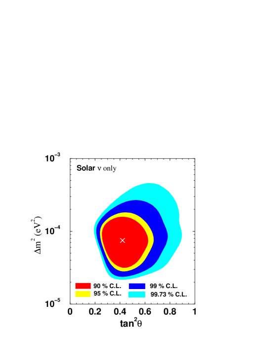
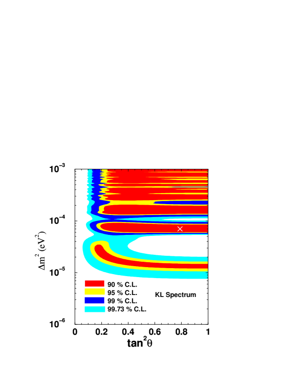
Figure 1: Region in $(\tan^{2}\theta,\Delta m^{2})$ plane allowed by the Super-Kamiokande-I zenith spectrum combined with rates from Homestake, GALLEX/GNO, SAGE and SNO. The best fit point is marked by a cross.

Figure 2: Regions in $(\tan^{2}\theta,\Delta m^{2})$ plane allowed by KamLAND data alone. The best fit point is marked by a cross.

In Figure 2 we show the region, in the $(\tan^{2}\theta,\Delta m^{2})$ plane, allowed by the Super-Kamiokande-I zenith spectrum data as well as by the rates of all other solar neutrino experiments at 90%, 95%, 99% and 99.73% C.L. In our fit we obtained a $\chi^{2}_{\odot}(\text{min})=37.7$ for 47 d.o.f (83 % C.L.), corresponding to the global best fit values $\Delta m^{2}=7.5\times 10^{-5}$ eV² and $\tan^{2}\theta=0.42$.

II.2 KamLAND

KamLAND kamland is a reactor neutrino oscillation experiment searching for $\bar{\nu}_{e}$ oscillation from over 16 power reactors in Japan and South Korea, mostly located at distances that vary from 80 to 344 km from the Kamioka mine, allowing KamLAND to probe the LMA MSW neutrino oscillation solution to the solar neutrino problem.

The KamLAND detector consists of about 1 kton of liquid scintillator surrounded by photomultiplier tubes that register the arrival of $\bar{\nu}_{e}$ through the inverse $\beta$-decay reaction $\bar{\nu}_{e}+p\to e^{+}+n$, by measuring $e^{+}$ and the 2.2 MeV $\gamma$-ray from neutron capture of a proton in delayed coincidence. The $e^{+}$ annihilate in the detector, producing the total visible energy $E$ which is related to the incoming $\bar{\nu}_{e}$ energy, $E_{\nu}$, as $E=E_{\nu}-(m_{n}-m_{p})+m_{e}$, where $m_{n}$, $m_{p}$ and $m_{e}$ are respectively, the neutron, proton and electron mass.

After 145.1 days of data taking, which corresponds to 162 ton yr exposure, KamLAND has measured 54 inverse $\beta$-decay events, where 87 were expected without neutrino conversion. These events are distributed in 13 bins of 0.425 MeV above the analysis threshold of 2.6 MeV (applied to contain the background under about 1 event).

We have theoretically computed the expected number of events in the $i$-th bin, $N_{i}^{\text{theo}}$, as

$$N_{i}^{\text{theo}}=\int dE_{\nu}\,\sigma(E_{\nu})\sum_{k}\phi_{k}(E_{\nu})P_{\nu_{e}\to\nu_{e}}\int_{i}dE\,R(E,E^{\prime}),$$ (2)

where $R(E,E^{\prime})$ is the energy resolution function, $E$ the observed and $E^{\prime}$ the true $e^{+}$ energy, with the energy resolution $7.5\%/\sqrt{E(\text{MeV})}$. Here $\sigma(E_{\nu})$ is the neutrino interaction cross-section and $\phi_{k}$ is the neutrino flux from the $k$-th power reactor, we have included all reactors with baseline smaller than 350 km in the sum. $P_{\nu_{e}\to\nu_{e}}\equiv P_{\bar{\nu}_{e}\to\bar{\nu}_{e}}$ (if CPT is conserved, which we will assume here) is the familiar neutrino survival probability in vacuum (the matter effect is negligible here), which is equal to one in case of no oscillation, and explicitly depends on $\Delta m^{2}$ and $\tan^{2}\theta$.

We were able to compute the region, in the $(\tan^{2}\theta,\Delta m^{2})$ plane, allowed by the KamLAND spectrum data, by minimizing with respect to these free parameters, the $\chi^{2}_{\text{KL}}$ function defined as $\chi^{2}_{\text{KL}}=\chi^{2}_{\text{G}}+\chi^{2}_{\text{P}}$ with

$$\chi^{2}_{\text{G}}=\displaystyle\sum_{i}\frac{(N_{i}^{\text{theo}}-N_{i}^{\text{obs}})^{2}}{\sigma_{i}^{2}},$$ (3)

and

$$\chi^{2}_{\text{P}}=\sum_{j}2(N_{j}^{\text{theo}}-N_{j}^{\text{obs}})+2\,N_{j}^{\text{obs}}\ln\displaystyle\frac{N_{j}^{\text{obs}}}{N_{j}^{\text{theo}}},$$ (4)

where $\sigma_{i}=\sqrt{N_{i}^{\text{obs}}+(0.0642\,N_{i}^{\text{obs}})^{2}}$ is the statistical plus systematic uncertainty in the number of events in the $i$-th bin and the sum in $i(j)$ is done over the bins having 4 or more (less than 4) events. We have also computed the allowed regions using purely Gaussian or Poissonian $\chi^{2}$ functions and found that the hybrid $\chi^{2}$ definition above could reproduce better KamLAND’s allowed regions kamland . Therefore, we have prefered to use it in our paper (see also Ref. valle ).

Using this $\chi^{2}_{\text{KL}}$ we have computed the allowed region at 90%, 95%, 99% and 99.73% C.L. shown in Fig. 2, which are quite consistent with the ones obtained by the KamLAND group in Fig. 6 of Ref. kamland . In our fit we obtained a $\chi^{2}_{\text{KL}}(\text{min})=5.4$ for 11 d.o.f (91 % C.L.), corresponding to the best fit values $\Delta m^{2}=7.0\times 10^{-5}$ eV² and $\tan^{2}\theta=0.79$.

II.3 Combined Results

Combining the results of all solar experiments with KamLAND data we have obtained the allowed region showed in Fig. 3. The minimum value of $\chi^{2}_{\text{tot}}=\chi^{2}_{\odot}+\chi^{2}_{\text{KL}}$ for the combined fit is $\chi^{2}_{\text{tot}}(\text{min})=43.6$ for 60 d.o.f (94.5 % C.L.), corresponding to the best fit values $\Delta m^{2}=7.1\times 10^{-5}$ eV² and $\tan^{2}\theta=0.42$. We observe that there are two separated regions which are allowed at 99 % C.L.: a lower one in $\Delta m^{2}$ (region 1) where the global best fit point is located, and an upper one (region 2) where the local best fit values are $\Delta m^{2}=1.5\times 10^{-4}$ eV² and $\tan^{2}\theta=0.41$, corresponding to $\chi^{2}_{\text{loc}}(\text{min})=49.2$. We observe that depending on the definition of $\chi^{2}_{\text{KL}}$ (gaussian, poisson or hybrid) used, a third tiny region above $\Delta m^{2}=2\times 10^{-4}$ eV² appears at 99.73% C.L. However, apart from this small change, the combined allowed region is not essentially affected by the $\chi^{2}_{\text{KL}}$ used.

In Fig. 4 we show the theoretically predicted energy spectra at KamLAND for no oscillation, the best fit values of the oscillation parameters for KamLAND data alone and for KamLAND combined with solar data in regions 1 and 2. We note that the fourth energy bin, which is for the moment below the analysis cut, can be quite important in determining the values of the oscillation parameters in the future.

III Future Perspectives

In this section we consider the effect of possible experimental improvements which can help in determining the oscillation parameters with more accuracy in the future. We first consider a reduction of the error in the SNO neutral-current measurement then an increase of event statistics in KamLAND.

III.1 Effect of reducing SNO neutral-current error

In order to constrain the solar neutrino oscillation parameters even more, in particular, to decide in which of the 99% C.L. islands $\Delta m^{2}$ really lie, we have investigated the effect of increasing the SNO neutral-current data precision to twice its current value. We have re-calculated the region, in the $(\tan^{2}\theta,\Delta m^{2})$ plane, allowed by all current solar neutrino data, artificially decreasing the SNO NC measurement error but keeping the current central value, as well as the other solar neutrino data, unchanged. The result can be seen in Fig. 6. The best fit point and the value of $\chi^{2}_{\odot}$(min) remain practically unchanged with respect to the result obtained in Sec. II.1, but the allowed region shrinks significantly. This is because the ${}^{8}B$ neutrino flux normalization, which can be directly inferred from SNO NC measurements, gets more constrained. Combining this with KamLAND data we obtain the allowed region shown in Fig. 6. We observe that this allowed region is substantially smaller compared to the one shown in Fig. 3. Moreover, region 2 only remains at 99% C.L.

III.2 Effect of increasing KamLAND statistics

We simulate the expected KamLAND spectrum after one year of data taking for three distinct assumptions. We have generated KamLAND future data compatible with the best fitted values of $\Delta m^{2}$ and $\tan^{2}\theta$ obtained for : (a) KamLAND data alone, (b) KamLAND and current solar neutrino data in region 1 and (c) KamLAND and current solar neutrino data in region 2. We have also included an extra bin, corresponding to the fourth bin in Fig. 4. We have re-calculated the region allowed by the combined fit with the current solar neutrino data in each case.

The results of our calculations can be seen in Figs. 8-9. If the future KamLAND result is close to the current one (see Fig. 8), values of $\tan^{2}\theta$ larger than the ones allowed now will be possible and region 2 will be excluded at 99% C.L. For this case we have obtained $\chi^{2}_{\text{tot}}$(min) $=42.1$. On the other hand, if the future KamLAND data are more compatible with the current best fit point of solar neutrino data (see Fig. 8), the global allowed region will diminish substantially with respect to Fig. 3 and region 2 will only remain at 99% C.L. For this case we have obtained $\chi^{2}_{\text{tot}}$(min) $=39.1$. Finally, if after one year KamLAND data is more compatible with region 2 (see Fig. 9) then one should observe an increase towards larger values of $\Delta m^{2}$ in the combined allowed region with respect to the one shown in Fig. 3. In this case region 1 and 2 will have similar statistical significance, corresponding to $\chi^{2}_{\text{tot}}$(min) $\sim 44.0$.

IV Discussions and Conclusion

We have performed a combined analysis of the complete set of solar neutrino data with the recent KamLAND result in a two neutrino flavor oscillation scheme. We have obtained, in agreement with other groups outros , two distinct islands, denominated regions 1 and 2, in the $(\tan^{2}\theta,\Delta m^{2})$ plane, which are the most probable regions where the true values of these parameters lie. Region 1, where the global best fit point was found, is around $\Delta m^{2}=7.1\times 10^{-5}$ eV², while region 2 is around $\Delta m^{2}=1.5\times 10^{-4}$ eV².

We have considered two possible future improvements in the determination of the neutrino oscillation parameters. First, we have investigated the effect of a 50 % decrease in the error of the SNO NC measurement. We have shown that this would substantially reduce the allowed parameter region when combined with KamLAND data. In particular, region 2 would not be allowed at 95% C.L. anymore.

Second, we have studied what can happen in the near future, when KamLAND collects 1 year of data. We have simulated the expected KamLAND spectrum including an extra lower bin, corresponding to the fourth bin in Fig. 3. Three different cases were studied in combination with the present solar neutrino data. In the first case, we have assumed that the future KamLAND spectrum will be compatible with oscillation parameter values at the best fit point for the present KamLAND data alone. This is the most restrictive case for region 2. In the second case, we have considered that future data will be more compatible with the present best fit point for the solar neutrino experiments. In this case, the combined allowed region will be much smaller than the present one and region 2 will be only allowed at 99% C.L. Finally, in the third case, we have assumed that the future KamLAND data will be compatible with the local best fit point in region 2. In this case, the combined allowed region will suffer an increase towards larger values of $\Delta m^{2}$ and region 1 and 2 will both have similar statistical significance.

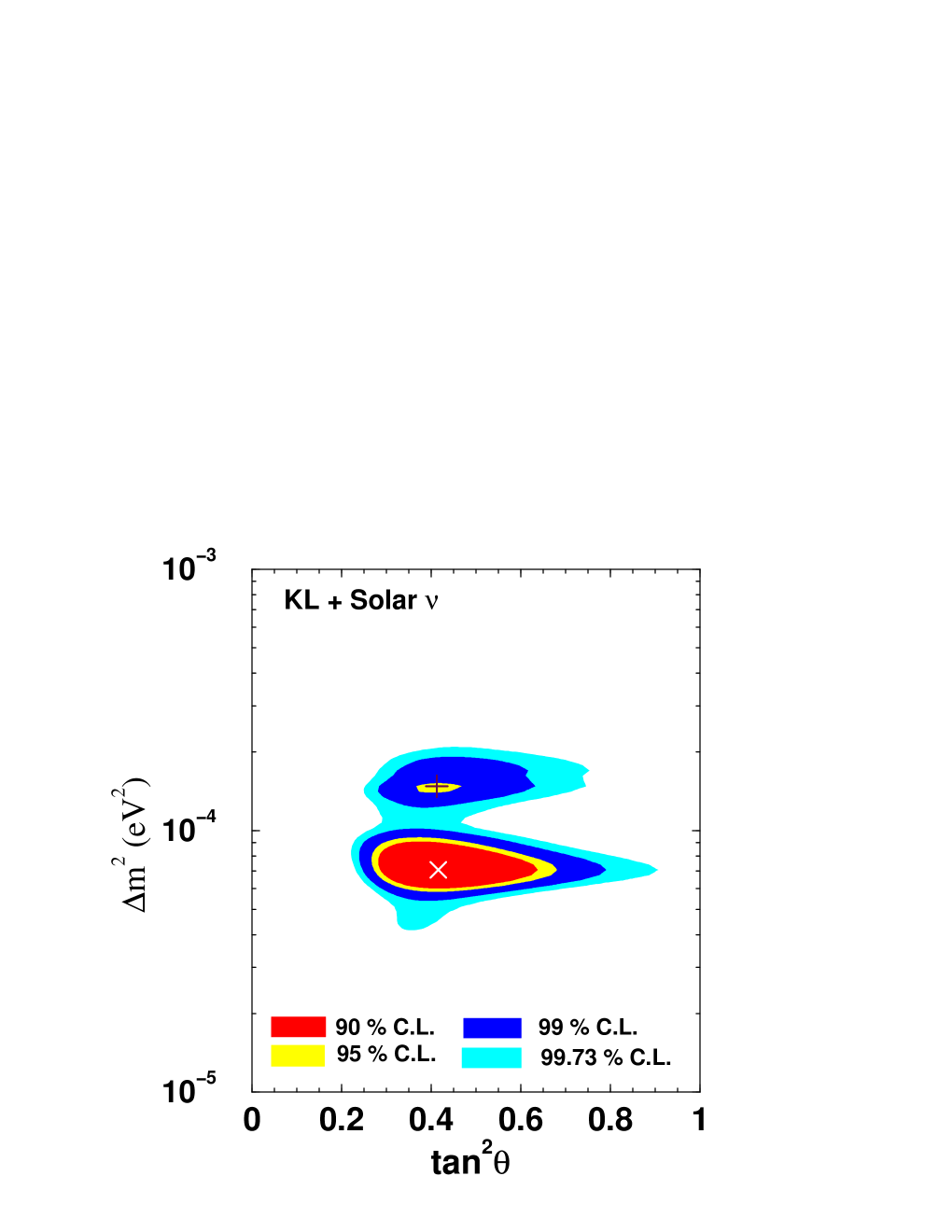
Figure 3: Region allowed by all the solar neutrino experiments combined with KamLAND (KL) data. The region below (above) $\Delta m^{2}=10^{-4}$ eV² is referred to as region 1 (2). The best fit points in each region are also marked by cross (global best) and plus (local best).

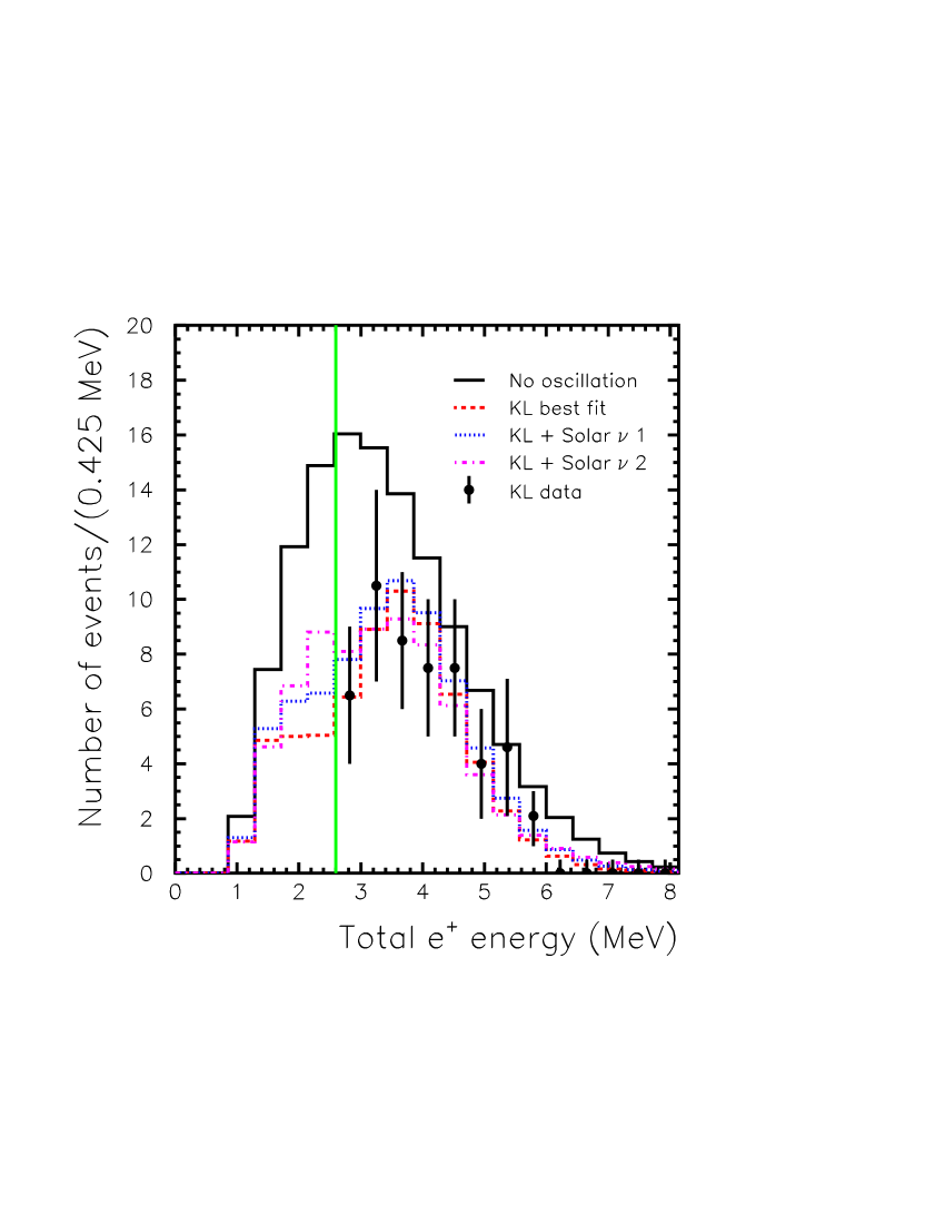
Figure 4: Expected positron energy spectra at KamLAND (KL) for no oscillation, the best fit values of the oscillation parameters for KamLAND data alone and KamLAND data combined with the solar neutrino data in regions 1 and 2 of Fig. 3. The KamLAND data kamland is also shown as solid circles with error bars. The energy threshold at 2.6 MeV is marked by a vertical line.

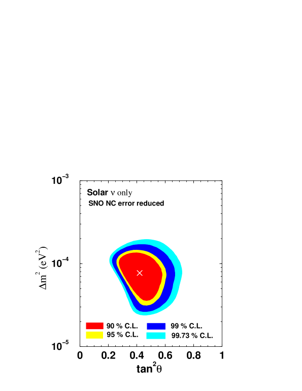
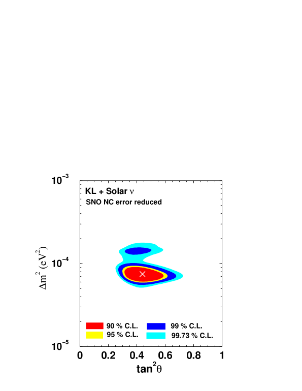
Figure 5: Same as Fig. 2 but decreasing the SNO neutral-current data error to half of its current value.

Figure 6: Same as Fig. 3 but decreasing the SNO neutral-current data error to half of its current value.

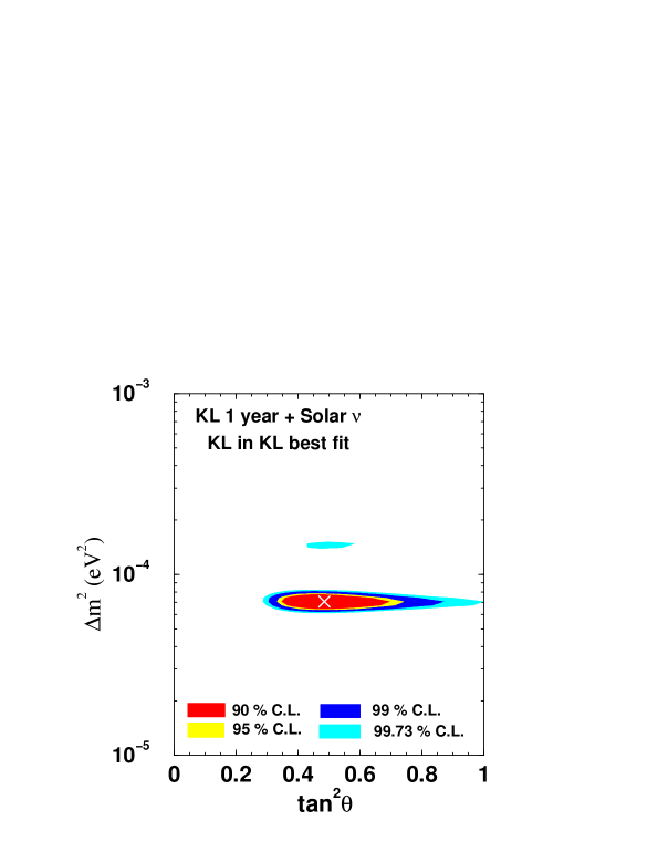
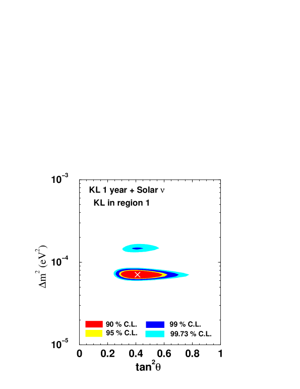
Figure 7: Same as Fig. 3 but for a simulated KamLAND spectrum after one year of data taking compatible with the KamLAND alone best fit $\Delta m^{2}=7\times 10^{-5}$ eV² and $\tan^{2}\theta=0.79$.

Figure 8: Same as Fig. 8 but for the KL + Solar neutrino global best fit $\Delta m^{2}=7.1\times 10^{-5}$ eV² and $\tan^{2}\theta=0.42$ in region 1.

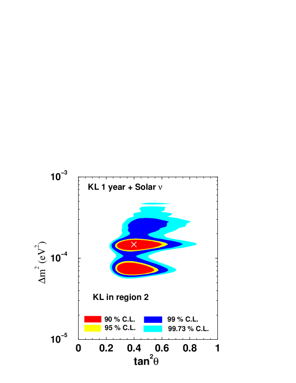
Figure 9: Same as Fig. 8 but for the KL + Solar neutrino local best fit $\Delta m^{2}=1.5\times 10^{-4}$ eV² and $\tan^{2}\theta=0.41$ in region 2.

- (1) Y. Fukuda et al. (Super-Kamiokande Collaboration), Phys. Rev. Lett. 81, 1562 (1998); H. S. Hirata et al. (Kamiokande Collaboration), Phys. Lett. B 205, 416 (1988); ibid. 280, 146 (1992); Y. Fukuda et al., ibid. 335, 237 (1994); R. Becker-Szendy et al. (IMB Collaboration), Phys. Rev. D 46, 3720 (1992); M. Ambrosio et al. (MACRO Collaboration), Phys. Lett. B 478, 5 (2000); B. C. Barish, Nucl. Phys. B (Proc. Suppl.) 91, 141 (2001); W. W. M. Allison et al. (Soudan-2 Collaboration), Phys. Lett. B 391, 491 (1997); Phys. Lett. B 449, 137 (1999); W. A. Mann, Nucl. Phys. B (Proc. Suppl.) 91, 134 (2001).
- (2) K2K Collaboration, S. H. Ahn et al., Phys. Lett. B 511, 178 (2001); K. Nishikawa, Talk presented at XXth International Conference on Neutrino Physics and Astrophysics (Neutrino 2002), May 25-30, 2002, Munich, Germany.
- (3) KamLAND Collaboration, K. Eguchi et al., Phys. Rev. Lett. 90, 021802 (2003); see also http://www.awa.tohoku.ac.jp/KamLAND/index.html.
- (4) J. N. Bahcall, M. C. Gonzalez-Garcia and C. Peña-Garay, JHEP 0207, 054 (2002); A. Bandyopadhyay et al., Phys. Lett. B 540, 14 (2002); V. Barger et al., Phys. Lett. B 537, 179 (2002); P. Aliani et al., AIP Conf. Proc. 655, 103 (2003) [arXiv:hep-ph/0211062]; P. C. de Holanda and A. Yu. Smirnov, Phys. Rev. D 66, 113005 (2002); P. Creminelli, G. Signorelli and A. Strumia, JHEP 0105, 052 (2001); G. L. Fogli et al., Phys. Rev. D 66, 053010 (2002); M. Maltoni et al., Phys. Rev. D 67, 013011 (2003).
- (5) A. M. Gago et al., Phys. Rev. D 65, 073012 (2002); M. Guzzo et al., Nucl. Phys. B 629, 479 (2002), and references therein.
- (6) Homestake Collaboration, B. T. Cleveland et al., Astrophys. J. 496, 505 (1998).
- (7) GALLEX Collaboration, W. Hampel et al., Phys. Lett. B 447, 127 (1999).
- (8) GNO Collaboration, M. Altmann et al., Phys. Lett. B 490, 16 (2000); T. Kirsten, on behalf of GNO Collaboration, talk presented at Neutrino 2002, May 25-30, Munich, Germany, see http://neutrino2002.ph.tum.de.
- (9) SAGE Collaboration, D. N. Abdurashitov et al., Nucl. Phys. (Proc. Suppl. ) 91, 36 (2001); Latest results from SAGE homepage: http://EWIServer.npl.washington.edu/SAGE/.
- (10) Super-Kamiokande Collaboration, S. Fukuda et al., Phys. Lett. B 539, 179 (2002).
- (11) SNO Collaboration, Q. R. Ahmad et al., Phys. Rev. Lett. 87, 071301 (2001); ibid. 89, 011301 (2002); 89, 011302 (2002).
- (12) S.P. Mikheyev and A. Yu. Smirnov, Yad. Fiz. 42, 1441 (1985) [Sov. J. Nucl. Phys. 42, 913 (1985)]; L. Wolfenstein, Phys. Rev. D 17, 2369 (1978).
- (13) J. N. Bahcall, Neutrino Astrophysics, Cambridge University Press, Cambridge, England, 1989.
- (14) S. J. Parke, Phys. Rev. Lett. 57, 1275 (1986); S. J. Parke and T. P. Walker, Phys. Rev. Lett. 57, 2322 (1986); J. Bouchez et al, Z. Phys. C 32 (1986) 499; M. Cribier et al., Phys. Lett. B182, 89 (1986); S. P. Mikheyev and A. Yu. Smirnov, Proc. of the 12th Int. Conf Neutrino’86 (Sendai, Japan) eds. T. Kitagaki and H. Yuta, 177 (1986) and Proc. of the Int. Symp. on Weak and Electromagnetic Interactions in Nuclei, WEIN-86, (Heidelberg, 1986), 710.
- (15) J. N. Bahcall, M. H. Pinsonneault and S. Basu, Astrophys. J. 555, 990 (2001).
- (16) M. Maltoni et al. in Ref. outros .
- (17) V. Barger and D. Marfatia, Phys. Lett. B 555, 144 (2003), G. L. Fogli, et al., arXiv:hep-ph/0212127; M. Maltoni, T. Schwetz and J. W. F. Valle, arXiv:hep-ph/0212129; A. Bandyopadhyay, et al., arXiv:hep-ph/0212146; J. N. Bahcall, M. C. Gonzalez-Garcia and C. Peña-Garay, JHEP 0302, 009 (2003).