KINETICS OF VACUUM PAIR CREATION IN STRONG ELECTROMAGNETIC FIELDS

Abstract

We study particle - antiparticle pair production under action of a strong time dependent space homogeneous electric field at the presence of a collinear constant magnetic field. We derive the kinetic equation for a such field configuration for fermions and bosons in the framework of the Schwinger mechanism of vacuum tunneling. We show the enhancement of pair production for fermions (suppression for bosons) with the increasing of the magnetic field as in the case of the constant electromagnetic field. We have constructed closed set of equations, which can be applied to some actual problems with manifestation of strong electromagnetic fields, e.g., it is essential in the framework of the Flux Tube Model of Quark - Gluon Plasma generation; for describing some cosmological objects and especially because of the planned experiments on creation of subcritical fields in the X-Free Electron Laser pulses.

1 Introduction

It is expected that the influence of a magnetic field on vacuum particle production at the presence of a non-stationary electric field can be essential in many physical situations. It should be mentioned, first of all, that the joint consideration of chromoelectric and chromomagnetic fields is necessary while constructing the Flux Tube Model(FTM) of superconductive type when describing the pre-equilibrium evolution of Quark - Gluon Plasma(QGP), generated under extreme conditions of ultra-relativistic heavy ion collisions [1, 10]. It is expected that extra-strong electromagnetic fields can exist in a series of astrophysical (e.g., magnetars) and cosmological (e.g., cosmic strings) objects. Finally, when achieving impact near-critical magnetic fields in a laboratory environment in comparatively short distances it would be very perspective to study combined action of electric and magnetic fields on vacuum $e^{+}e^{-}$ pair creation, e.g., under conditions of the planned experiment on the X-Free Electron Laser(X-FEL) [2].

Electron-positron pair production in constant electromagnetic(EM) fields was considered in the work [3] (see also [4]). Here we will assume the electric field is time dependent (but the magnetic field remains constant). For derivation of the kinetic equation (KE) we will use non-perturbative approach developed in works[5].

2 Solution of the one-particle problem

We consider $e^{+}e^{-}$ vacuum pair creation under action of the external EM field with the configuration of vector potential of the kind

$$A^{\mu}(\vec{x},t)=\left(0,0,-Hx^{1},A^{3}(t)=A(t)\right)\,,$$ (1)

where $H$ is the strength of the magnetic field, so that we have space homogeneous EM field, polarized in one direction. The electric field is time dependent, whereas the magnetic field is constant,

$$\vec{E}(t)=\left(0,0,E^{3}(t)=-\dot{A}^{3}(t)\right),\qquad\vec{H}=(0,0,H)\,,$$ (2)

where dot denotes time derivative.

The squared Dirac Equation is $\left(D^{2}+m^{2}+\frac{ie}{2}F_{\mu\nu}\gamma^{\mu}\gamma^{\nu}\right)\Psi=0,$ where $F_{\mu\nu}=A_{\nu,\mu}-A_{\mu,\nu}$, $D_{\mu}=\partial_{\mu}-ieA_{\mu}$ and $-e$ is the electron charge. This equation in the chosen configuration of fields (1) has the form

$$(\partial^{2}_{0}-\triangle+m^{2}+2ie[Hx^{1}\partial_{2}-A\partial_{3}]+e^{2}[H^{2}(x^{1})^{2}+A^{2}]+$$

$$+ie[\partial_{0}A\gamma^{0}\gamma^{3}-H\gamma^{1}\gamma^{2}])\Psi=0\,.$$ (3)

Let us choose solution in the form

$$\Psi_{r}(\vec{x},t)=CT(t)\Psi(x_{1})e^{i(p^{2}x^{2}+p^{3}x^{3})}R_{r}\,,$$ (4)

where $C$ is a normalizing constant and $R_{r}(r=1,2)$ are Nikishov spinors [3, 4]:

$$R_{1}^{+}=(0,1,0,-1),\qquad R_{2}^{+}=(1,0,1,0)\,.$$ (5)

The result of separation of variables gives the time-dependent part

$$\left\{\partial^{2}_{0}+\omega^{2}_{r\lambda}(\vec{p},t)+ie\partial_{0}A\right\}T_{\lambda r}(t)=0\,,$$ (6)

and space-dependent part

$$\left\{\partial^{2}_{1}+2ex^{1}p^{2}H-e^{2}(x^{1})^{2}H^{2}+\lambda\right\}\Psi(x^{1})=0\,,$$ (7)

where $\lambda$ is a separation constant and

$$\omega^{2}_{r\lambda}(\vec{p},t)=(p^{2})^{2}+(p^{3}+eA)^{2}+m^{2}-e(-1)^{r}H+\lambda\,.$$

Eq. (7) can be reduced to

$$\Psi^{\prime\prime}_{n}(\eta)+(2n+1-\eta^{2})\Psi_{n}(\eta)=0,\,\,\mbox{with}\,\,\eta=\sqrt{eH}\left(x^{1}-\frac{p^{2}}{eH}\right)\,,$$ (8)

where prime means derivative with respect to $\eta$.

The solution of Eq. (8) is known

$$\Psi_{n}(\eta)=exp(-\eta^{2}/2)H_{n}(\eta),\,\,\mbox{with}\,\,\lambda_{n}=(2n+1)eH\,,$$ (9)

where $H_{n}$ are Chebyshev-Hermite polynomials and we have solutions

$$\Psi^{(\pm)}_{np^{2}p^{3},r}(\vec{x},t)=C_{n}T^{(\pm)}_{nr}(t)exp(-\eta^{2}/2)H_{n}(\eta)e^{i(p^{2}x^{2}+p^{3}x^{3})}R_{r}\,,$$ (10)

where $(\pm)$ signs correspond to positive and negative frequency solutions of the equation (6) and we have introduced the kinetic momentum $P=p^{3}+eA(t)$ and one particle energy $\omega^{2}_{rn}(P)=P^{2}+m^{2}+eH[2n+1+(-1)^{r}]$.

Finally, the normalization conditions are

$$\int d^{3}x\bar{\Psi}^{(\pm)}_{np^{2}Pr}(\vec{x},t)\Psi^{(\pm)}_{n^{\prime}p^{\prime 2}P^{\prime}r^{\prime}}(\vec{x},t)=\delta_{nn^{\prime}}\delta_{rr^{\prime}}\delta(p^{2}-p^{\prime 2})\delta(P-P^{\prime})\,,$$ (11)

with normalization constant $C_{n}=\left(\frac{eH}{\pi}\right)^{1/4}\frac{1}{2\pi}(2^{n+1}n!)^{-1/2}$.

Functions (10) form the complete system of orthonormalized functions. That is enough for the construction of the secondary quantized representation with the field operator

$$\Psi(x)=\sum_{r,n}\int dP\left\{\Psi^{(-)}_{np^{2}Pr}(\vec{x},t)a^{(-)}_{np^{2}Pr}+\Psi^{(+)}_{np^{2}Pr}(\vec{x},t)a^{(+)}_{np^{2}Pr}\right\}\,,$$ (12)

where $a^{(-)},a^{*(+)}$ are annihilation and creation operators with the standard set of anti-commutation relations.

3 The kinetic equation in the quasi-particle representation

The Kinetic Equation(KE) derivation requires the transition to the quasi-particle representation, which is archived by the diagonalization procedure of the Hamiltonian. In the considered case the procedure is distinguished from the usual one [4] only in some details, concerned with the specific character of basis functions (10). Let the new operators $b^{(-)}(t)$ and $b^{*(+)}(t)$ are annihilation and creation operators in the quasi-particle representation, connected with $a^{(-)}$ and $a^{*(+)}$ operators by the time dependent Bogoliubov transformation [4]. Then it is possible to introduce the distribution function of electrons in the new representation with the momentum $p^{2},P$ and spin $r$ on the Landau $n$- level

$$f_{nr}(p^{2},P,t)=\langle 0_{in}|b^{*(+)}_{np^{2}Pr}(t)b^{(-)}_{np^{2}Pr}(t)|0_{in}\rangle$$ (13)

and the corresponding distribution function of positrons $\bar{f}_{nr}(p^{2},P,t)$ with an electric neutrality condition $f=\bar{f}$.

The KE derivation for function (13) differs from the case of $H=0$ [5] only in some details concerned with the source term describing the processes of vacuum tunneling. Now we have

$$\dot{f}_{nr}(P,t)=S_{nr}(P,t)\,,$$ (14)

where source of pair production is

$$\begin{array}[]{lcl}&&S_{nr}(p^{2},P,t)=S_{nr}(P,t)=\frac{1}{2}w_{nr}(P,t)\times\\ \\ &\times&\int^{t}_{-\infty}dt^{\prime}w_{nr}(P(t,t^{\prime}),t^{\prime})[1-2f_{nr}(P,t^{\prime})]\cos{\left\{2\int^{t}_{t^{\prime}}d\tau\omega_{nr}(P,\tau)\right\}}\,,\end{array}$$ (18)

where $P(t,t^{\prime})=P-e\int^{t}_{t^{\prime}}d\tau E(t)\,$ and

$$w_{nr}(P,t)=\frac{eE(t)\varepsilon_{nr}}{\omega^{2}_{nr}(P)}\,,$$ (19)

where $\varepsilon^{2}_{nr}=m^{2}+eH[1+2n+(-1)^{r}]$.

As one can see from Eqs. (18)-(19) the distribution function does not depend on $p^{2}$, $f_{nr}(p^{2},P,t)=f_{nr}(P,t)$ (the cylindrical symmetry of the considered problem). This circumstance was taken into account in the KE Eq. (14).

The comparison of the source term (18)-(19) with the ”old” case $H=0$ [5] shows that the ”new” quasi-particle frequency $\omega_{rn}$, transition amplitude (19) and transversal energy $\varepsilon_{nr}$ can be obtained from the corresponding ”old” formulas by means of formal substitution

$$(p^{1})^{2}+(p^{2})^{2}=p^{2}_{\bot}\rightarrow eH[1+2n+(-1)^{r}]\,,$$ (20)

which provides discrete transversal energy as in the case with boundary conditions [8]

For numerical analysis it is convenient to reduce the KE (14)-(19) to the following system of ordinary differential equations:

$$\dot{f}_{nr}(P,t) = \frac{1}{2}w_{nr}(P,t)v_{nr}(P,t)\,,$$

$$\dot{v}_{nr}(P,t) = w_{nr}(P,t)(1-2f_{nr}(P,t))-2\omega_{nr}(P,t)z_{nr}(P,t)\,,$$ (21)

$$\dot{z}_{nr}(P,t) = 2\omega_{nr}(P,t)v_{nr}(P,t)\,,$$

where $v$ and $z$ are auxiliary functions.

4 Scalar particle production

The Klein- Gordon equation in the field (1) permits the separation of variables as well

$$\varphi^{\pm}(x)=T^{\pm}(t)\Phi(x_{1})e^{ip^{2}x^{2}+ip^{3}x^{3}}\,,$$ (22)

where functions $T(t)$ and $\Phi(x_{1})$ satisfy following equations

$$\ddot{T}^{\pm}+\omega^{2}_{\lambda}(t)T^{\pm}=0\,,\qquad\Phi^{\prime\prime}(\eta)-\eta^{2}\Phi(\eta)+\frac{\lambda+(p^{2})^{2}}{|e|H}\Phi(\eta)=0\,,$$ (23)

where now $\eta=\sqrt{|e|H}\left(x^{1}+p^{2}/|e|H\right)$. Normalized solutions of the last equation are again Chebyshev-Hermite polynomials with $\lambda_{n}+(p^{2})^{2}=(2n+1)|e|H$ , $n=0,1,\ldots$. Functions $T^{\pm}(t)$ are positive and negative solutions of (23) and we can write a formal solution

$$\varphi^{\pm}_{n,p^{2},p^{3}}(x)=C_{n}T^{\pm}_{n}(t)exp(-\eta^{2}/2)H_{n}(\eta)e^{i(p^{2}x^{2}+p^{3}x^{3})},$$ (24)

where a normalization constant is $C_{n}=\frac{1}{2\pi}\left(\frac{|e|H}{\pi}\right)^{1/4}\left(2^{n}n!\right)^{-1/2}$, which can be obtained from the condition

$$i\int d^{3}x\varphi^{(\pm)*}_{n,p^{2},p^{3}}(x)\stackrel{{\scriptstyle\leftrightarrow}}{{\partial}}(t)\varphi^{\pm}_{n^{\prime},p^{2^{\prime}},p^{3^{\prime}}}(x)=\mp\delta_{nn^{\prime}}\delta(p^{2}-p^{2^{\prime}})\delta(p^{3}-p^{3^{\prime}}).$$

One can obtain the KE (14) by analogy with the above considered case, assuming $r=0$,

$$S_{n}(,P,t)=\frac{1}{2}w_{n}(P,t)\times$$

$$\times\int\limits^{t}_{-\infty}dt^{\prime}w_{n}((P,t^{\prime}),t^{\prime})[1+2f_{n}(P,t^{\prime})]\cos\left\{2\int_{t^{\prime}}^{t}d\tau\omega_{n}(P,\tau)\right\}\,,$$ (25)

where $\omega^{2}_{n}(P,t,t^{\prime})=m^{2}+P^{2}(t,t^{\prime})+|e|H(2n+1)$ and

$$w_{n}(P,t)=\frac{|e|E(t)P(t)}{\omega_{n}(P,t)}\,.$$ (26)

5 Back reaction problem

For the description of the back reaction problem it is necessary to add the regularized Maxwell equation. It follows from Eq. (19) that $w\sim P^{-2}$ at $P\rightarrow\infty$. It leads to the absence of ultraviolet divergences in the densities of observed quantities, which are expressed by means of integrals containing the function $f_{nr}(P,t)$. However, there is divergence of the sum over levels $n$ and corresponding counter terms should subtracted while calculating densities of physical values.

In order to construct counter-terms according to the procedure of n-wave regularization [4, 6], it is necessary to expand functions $f$,$v$ and $z$ in asymptotic series under inverse powers of one particle energy $\omega_{\alpha}$. After application of this procedure to the set of Eqs. (3) we obtain leading contributions

$$v^{\alpha}_{3}(t)=\frac{e\dot{E}(t)P}{4\omega_{\alpha}(P,t)}\bigg{(}\frac{\epsilon_{\alpha}}{P}\bigg{)}^{g_{\alpha}-1}\,,\qquad f^{\alpha}_{4}(t)=\left(\frac{eE(t)P}{4\omega_{\alpha}(P,t)}\bigg{(}\frac{\epsilon_{\alpha}}{P}\bigg{)}^{g_{\alpha}-1}\right)^{2}\,,$$

where $g_{\alpha}$ is the degeneracy factor for corresponding set $\alpha$ of quantum numbers $\{n,r\}$ or $\{n\}$.

The counter term is similar to the case $H=0$ [9] and sum diverges logarithmically at $n\rightarrow\infty$ for fermions and at $|P|\rightarrow\infty$ for scalar particles. Thus, we find that the mean number density of $e^{+}e^{-}$ pairs

$$n(t)=\sum_{nr}(P)f_{nr}(P,t)$$

is finite, whereas the mean energy density and the total current density as the sum of the conduction and the vacuum polarization currents contain divergences, which can be eliminated with the help of counter terms:

$$\varepsilon(t)=2\sum_{nr}(P)\left\{\omega_{nr}(P)(f_{nr}(P,t)-f_{c}(P,t))\right\}\,,$$ (27)

$$j^{-}(t)=2e\sum_{nr}(P)\frac{1}{\omega_{nr}(P)}\left\{Pf_{nr}(P,t)+\frac{1}{2}\varepsilon_{nr}\left(v_{nr}(P,t)-v_{c}(P,t)\right)\right\}\,,$$ (28)

Expressions (27) and (28) are renormalized according to charge renormalization procedure [6, 9]. Here we have the short notation

$$\sum_{nr}(P)=\frac{eH}{(2\pi)^{2}}\sum_{r=1}^{g_{\alpha}}\sum_{n=0}^{\infty}\int_{-\infty}^{\infty}dP\,.$$ (29)

The factor $eH$ describes the degeneracy of the distribution function (13) relatively of $p_{\bot}$ [7].

The Eqs. system (3) with the Maxwell Eq. $\dot{E}=-j^{\alpha}(t)$ compose the complete equation system of back reaction problem.

6 Conclusion and numerical results

The creation of scalar particle in the time dependent electric field with the presence of the strong collinear magnetic field is accompanied by the increase of effective mass $m\rightarrow m^{*}_{n}=\left(m^{2}+|e|H(2n+1)\right)^{1/2}$, so that we have even in the basic state $m^{*}_{n=0}>m$. This circumstance decreases the vacuum production of scalar bosons in the magnetic field [4].

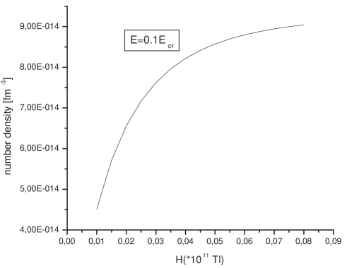
Figure 1: Number density of fermions for $\vec{E}=(0,0,E_{0}cosh^{-2}(t/b))$, $b=0.5$ as a function of magnetic field strength.

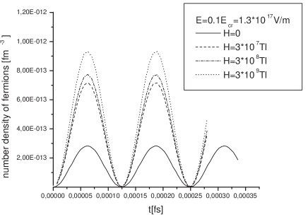
Figure 2: Time evolution of fermionic number density for $\vec{E}=(0,0,E_{0}sin(\Omega t))$, with $\Omega~{}=~{}8~{}\cdot~{}10^{18}\pi\ s^{-1}$, $\vec{H}=(0,0,H)$.

Another situation is in the fermionic case: as it follows from (19), the effective mass coincides with the particle mass for the spin states of electrons oriented opposite to the magnetic field. That leads to paramagnetism of $e^{+}e^{-}$ plasma, created from vacuum by the EM field (1). When spin oriented along the magnetic field direction then the effective mass $m_{2}^{*}=(m^{2}+2|e|Hn)^{1/2}$ and vacuum creation of such electrons and positrons are suppressed. However, the creation of the electrons in the state with $r=1$ with effective mass $m^{*}_{1}=m$ turns out more intensive in comparison with the case of an absence of magnetic field (this fact is well known for constant EM fields [4]). In Fig. 1 we show the number density of $e^{+}e^{-}$ pairs after action of external electric field impulse as a function of magnetic field strength. In Fig. 2 we show the time evolution of number density in alternating external electric field at various magnetic field strength.

References

- [1] M.A. Lampert and B. Svetitsky, Phys. Rev. D 61, 034011 (2000).
- [2] V.S.Popov, JETP Letters, 74, 133 (2001); K.Dietz and M.Probsting, nucl-th/9712067; R. Alkofer, M. B. Hecht, C. D. Roberts, S. M. Schmidt and D. V. Vinnik, Phys. Rev. Lett. 87, 193902 (2001); C. D. Roberts, S. M. Schmidt and D. V. Vinnik, Phys. Rev. Lett. 89, 153901 (2002).
- [3] A.I. Nikishov, JETPh, 57, 1210 (1969).
- [4] A.A. Grib, S.G. Mamaev and V.M. Mostepanenko, Vacuum quantum effects in strong external fields, (Atomizdat, Moscow, 1988).
- [5] S.M.Schmidt, D.Blaschke, G.Röpke, S.A.Smolyansky, A.V.Prozorkevich, V.D.Toneev, Int.J.Mod.Phys. E7,709 (1998); Phys. Rev. D59, 094005 (1999).
- [6] J.C.Bloch, V.A.Mizerny, A.V.Prozorkevich, C.D.Roberts, S.M.Schmidt, S.A.Smolyansky, D.V.Vinnik, Phys. Rev. D60, 1160011 (1999).
- [7] L.D.Landau and E.M.Lifshits, Statistical Physics (Nauka, Moscow (1976)).
- [8] D. V. Vinnik, R. Alkofer, S. M. Schmidt, S. A. Smolyansky, V. V. Skokov and A. V. Prozorkevitch, Few Body Syst. 32, 23 (2002).
- [9] D. V. Vinnik, A. V. Prozorkevich, S. A. Smolyansky, V. D. Toneev, M. B. Hecht, C. D. Roberts, S. M. Schmidt, Eur. Phys. J. C 22, 341 (2001).
- [10] C. D. Roberts and S. M. Schmidt,Prog. Part. Nucl. Phys. 45, S1 (2000).
Index
- back reaction §5, §5