Abstract

We present a study of $\alpha_{\rm MOM}(p)$ at small $p$ computed from the lattice. It shows a dramatic $\propto p^{4}$ law which can be understood within an instanton liquid model. In this framework the prefactor gives a direct measure of the instanton density in thermalised configurations. A preliminary result for this density is $5.27(4)\,{\rm fm}^{-4}$.

P.A.C.S.: 12.38.Aw; 12.38.Gc; 12.38.Cy; 11.15.H

1 Introduction

In a series of lattice studies [1]-[5] the gluon propagator in QCD has been computed at large momenta, and it was shown that its behavior was compatible with the perturbative expectation provided a rather large $1/p^{2}$ correction was considered. In an OPE approach this correction has been shown [3, 4] to stem from an $A^{2}$ gluon condensate which has not to vanish since the calculations are performed in the Landau gauge.

In the deep infrared (IR) region, where the perturbative approach is completely meaningless, the present knowledge of the coupling constant is not so clear, in spite of all the effort that has been dedicated for years (See [6] and references therein).

Lattice calculations provide a unique laboratory to obtain the behavior of the coupling at scales below the hadronization scale, where a complete understanding of the non-perturbative coupling would be a very important step towards the comprehension of hadronization. In this framework, the non-perturbative coupling has been computed from different vertices, the quark-gluon vertex [7], the ghost-gluon vertex [8], the three-gluon vertex[9, 2], different propagators [2, 10], etc.

Instantons [11] have been proposed, via the instanton liquid picture, to describe a number of non-perturbative phenomena in QCD, and particularly to explain the low part of the Dirac operator spectrum and hence the genesis of the chiral Goldstone boson, see [12]-[15] to mention only a few papers.

Instanton studies on the lattice have used essentially the cooled gauge configurations, [16]-[21], which allow to see instanton-like structures. These results have been used to introduce a new definition of the strong coupling constant in the IR [22].

This cooling method has been criticized [23] as creating a distortion on the original thermalised gauge configuration, and it was claimed that a direct study of the local chirality on a thermalized gauge configuration contradicted the instanton liquid picture. However other authors, [24, 25], concluded from a similar analysis that the dominance of instantons on topological charge fluctuations is not ruled out by local chirality measurements.

In this letter we study another observable, namely the strong coupling constant $\alpha_{\rm MOM}$ in the deep IR region on thermalised gauge configurations and we show that it strongly supports the instanton liquid picture.

Simultaneously we think that we provide a very simple and appealing understanding of the IR behavior of $\alpha_{\rm MOM}$. This tends to confirm the claim presented in [5] that an instanton liquid might explain the $<A^{2}>$ condensate observed via power corrections to the perturbative behavior of the gluon propagator and $\alpha_{\rm MOM}$ in the large momentum regime.

We will recall the lattice definition of $\alpha_{\rm MOM}$, derive the behavior of $\alpha_{\rm MOM}$ in an instanton liquid and compare the latter with numerical results in the low momentum region. We then use cooled gauge configurations to compare, as a test, the instanton density derived from $\alpha_{\rm MOM}$ to that which is directly observed from shape recognition. We then conclude.

2 Instanton background effect on $\alpha_{\rm MOM}$

2.1 Non-perturbative definition of $\alpha_{\rm MOM}$

Let us recall shortly the non-perturbative MOM definition of $\alpha_{s}(p^{2})$ [9, 2] in Landau gauge. We consider the three-gluon Green function ${G^{(3)}}_{\mu_{1}\mu_{2}\mu_{3}}^{a_{1}a_{2}a_{3}}(p_{1},p_{2},p_{3})$ at the symmetric point, $p_{1}^{2}=p_{2}^{2}=p_{3}^{2}\equiv\mu^{2}$.

The tree-diagram three-gluon vertex is given by $g_{s}\,T^{tree}$ with $T^{tree}$ defined by

$$T^{tree}_{\mu_{1}\mu_{2}\mu_{3}}=\big{[}\delta_{\mu_{1}^{\prime}\mu_{2}^{\prime}}(p_{1}-p_{2})_{\mu_{3}^{\prime}}+\hbox{cycl. perm.}\big{]}\prod_{i=1,3}\left(\delta_{\mu_{i}^{\prime}\mu_{i}}-\frac{p_{i\,\mu_{i}^{\prime}}p_{i\,\mu_{i}}}{p_{i}^{2}}\right)$$ (1)

The three-gluon Green function may be expanded on a basis of tensors. We are interested in the scalar function $G^{(3)}(\mu^{2},\mu^{2},\mu^{2})$ which multiplies $T^{tree}$. It is obtained by the following contraction

$$G^{(3)}(\mu^{2},\mu^{2},\mu^{2})=\frac{-i}{18\mu^{2}}\,\frac{f^{a_{1}a_{2}a_{3}}}{24}\,{G^{(3)}}_{\mu_{1}\mu_{2}\mu_{3}}^{a_{1}a_{2}a_{3}}(p_{1},p_{2},p_{3})$$

$$\left[T^{tree}_{\mu_{1}\mu_{2}\mu_{3}}+\frac{(p_{1}-p_{2})_{\mu_{3}}(p_{2}-p_{3})_{\mu_{1}}(p_{3}-p_{1})_{\mu_{2}}}{2\mu^{2}}\right]$$ (2)

The Euclidean two point Green function in momentum space writes in the Landau Gauge:

$${G^{(2)}}_{\mu_{1}\mu_{2}}^{a_{1}a_{2}}(p,-p)=G^{(2)}(p^{2})\delta_{a_{1}a_{2}}\left(\delta_{\mu_{1}\mu_{2}}-\frac{p_{\mu_{1}}p_{\mu_{2}}}{p^{2}}\right)$$ (3)

where $a_{1},a_{2}$ are the color indices ranging from 1 to 8.

Then the renormalised coupling constant is given by [9]

$$g_{R}(\mu^{2})=\frac{G^{(3)}(p_{1}^{2},p_{2}^{2},p_{3}^{2})Z_{3}^{3/2}(\mu^{2})}{G^{(2)}(p_{1}^{2})G^{(2)}(p_{2}^{2})G^{(2)}(p_{3}^{2})}$$ (4)

where

$$Z_{3}(\mu^{2})=G^{(2)}(\mu^{2})\mu^{2}$$ (5)

2.2 Solution in an instanton liquid

Let us consider an instanton liquid picture [12]-[15] i.e. a gauge field given by

$$A_{\mu}^{(I)a}({\bf x})=\sum_{i}R^{a\alpha}_{(i)}\,\overline{\eta}^{\alpha}_{\mu\nu}{(x_{\nu}-z_{\nu}^{i})}\ \rho_{i}^{-2}P\left(\frac{(x-z^{i})^{2}}{\rho_{i}^{2}}\right)\ ,$$ (6)

where $z^{i}$ ($\rho_{i}$) are the center (radius) of the instantons, $\overline{\eta}^{\alpha}_{\mu\nu}$ is known as ’t Hooft symbol, $R^{a\,\alpha}_{(i)}$ are color rotations embedding the canonical $SU(2)$ instanton into the $SU(3)$ gauge group, $\alpha=1,3$ ($a=1,8$) is an $SU(2)$ ($SU(3)$) color index, and the sum is extended over instantons and anti-instantons.

In order to take into account instanton deformation resulting from their interaction  we do not assume that the radial function $P(u)$ is equal to $2/(u^{2}(u^{2}+1))$ as for ’t Hooft-Polyakov’s instanton.

The field’s Fourier transform is

$$\widetilde{A_{\mu}^{(I)a}}({\bf p})=i\sum_{i}R^{a\alpha}_{(i)}\overline{\eta}^{\alpha}_{\mu\nu}e^{ik\cdot z^{i}}\rho_{i}^{3}\frac{p_{\nu}}{p}I(p\rho_{i})$$ (7)

for $p\neq 0$ and $\widetilde{A_{\mu}^{(I)a}}(0)=0$. The function $I(p\rho_{i})$ is given by

$$I(s)\ =\frac{4\pi^{2}}{s}\int_{0}^{\infty}\ z^{3}dzJ_{2}(sz)\,P(z)\ ;$$ (8)

$J_{2}$ being the second order Bessel J function.

From eqs. (3), (7) and the relation

$${G^{(2)}}_{\mu\nu}^{ab}(p)=\frac{1}{V}<\widetilde{A_{\mu}^{a}}({\bf p})\widetilde{A_{\mu}^{b}}({\bf-p})>$$ (9)

where the average $<\cdots>$ stands here for the average over instantons, we get

$$G^{(2)}(p^{2})=\frac{n}{8}<\rho^{6}I(p\rho)^{2}>$$ (10)

$n$ being the instanton density and $\rho$ being the instanton radius. When computing the result in eq. (10) we have used the relations concerning the ${\eta}$ tensors from the appendix A in ref. [12] and the orthogonality relation

$$\sum_{a}R^{a\alpha}_{(i)}R^{a\beta}_{(i)}=\delta^{\alpha,\beta}\qquad<\sum_{a}R^{a\alpha}_{(i)}R^{a\beta}_{(j)}e^{ip(z_{i}-z_{j})}>_{i\neq j}\simeq 0\,\,$$ (11)

For brevity we skip the derivation of the first of these equations. The second one is not exact but expresses the hypothesis  that the color rotations are at random for different instantons as well as the phases $e^{ip(z_{i}-z_{j})}$. The cross-products are thus reasonably assumed to average to zero.

Similarly,

$$G^{(3)}(p^{2},p^{2},p^{2})=\frac{n}{48\,p}<\rho^{9}I(p\rho)^{3}>$$ (12)

where we have used again ref. [12] and

$$\sum_{abc}R^{a\alpha}_{(i)}R^{b\beta}_{(i)}R^{c\gamma}_{(i)}f_{abc}=\epsilon^{\alpha\beta\gamma}.$$ (13)

We skip again the derivation of this equation and again we neglect crossed terms for the same reason as in (11). The strong coupling constant is then given by

$$\alpha_{\rm MOM}(p)\equiv\frac{g_{R}^{2}}{4\pi}=\frac{1}{4\pi}\left[\frac{G^{(3)}(p^{2},p^{2},p^{2})}{(G^{(2)}(p^{2}))^{3}}(p^{2}G^{(2)}(p^{2}))^{3/2}\right]^{2}=\frac{1}{18\pi}n^{-1}p^{4}$$ (14)

where we have assumed, for simplicity, that all the instantons have equal radii; this will be discussed later. The very remarkable feature of this result is that it does not depend on the shape of the instanton-like structures i.e. on the function $I$ (that has all the information about the profile function $P(u)$), neither on the scale $\rho$ appearing in (6) i.e. on the instanton radius. It only depends on the instanton density $n$.

3 Lattice three gluon vertex.

In several lattice works, the scheme outlined in 2.1 has been used [2] to compute the running coupling constant in a quite wide range of lattice volumes and spacings. The region of high momenta has been precisely described according to the perturbative running plus non-perturbative corrections in an Operator Product Expansion framework (Figure 1(b)).

The smaller momenta, on the contrary, are not yet theoretically understood. The aim of this paper is to try an instanton interpretation at very low momentum, as far as possible from the perturbative regime. We will therefore make a fit of the deep IR region combining all points from different lattice settings in order to achieve enough statistics. The use of different lattice settings, with varying statistics, makes it difficult to estimate the errors with the usual jacknife method. Therefore, calling $\chi_{\rm min}^{2}$ the minimum $\chi^{2}$, we estimate the errors by assuming that one standard deviation is reached when $\chi^{2}=\chi_{\rm min}^{2}+1$ while, of course, the central value corresponds to $\chi^{2}=\chi_{\rm min}^{2}$.

A quick inspection of the points in fig. 1(a) shows that even for very small momenta the scaling is very good, i.e. the simulations with different lattice spacings agree strikingly. We have used unusually low values of $\beta$ i.e. unusually large lattice spacings - and hence large volumes - in order to reach small momenta. The quality of the scaling for these small momenta as well as for larger ones makes us confident that we do not introduce a sizable bias with these small $\beta$’s. We take the ratios between lattice spacings for different $\beta$’s from ref. [27] and $a^{-1}(\beta=6.0)=1.97$ GeV.

If we fit the low tail of the coupling (up to momenta $\sim 0.8\ {\rm GeV}$) by a power law, a power $3.84(8)$ is obtained, in good agreement with the expected power-four behavior.

Fixing now the power to be four, the density resulting from formula (14) is $n=5.27(4){\rm fm}^{-4}$, with $\chi^{2}/d.o.f.=3.8$ (Figure 1(a)). This is in the right ballpark since several arguments [26] point toward a few ${\rm fm}^{-4}$’s. The rather large $\chi^{2}/d.o.f.=3.8$ is due to two points which have unusually small errors, maybe because of the small statistics used in this preliminary study. Furthermore an exact power 4 should not be taken too seriously since the instanton radii distribution can presumably distort this power law. Indeed the dispersion of the ’t Hooft instanton radii leads to an effective power smaller than four at small momenta, but the deviation from four is small.

So within this approach, we are able to compute the instanton density directly from the thermalised lattice, and we obtain a result which is not biased by a cooling procedure.

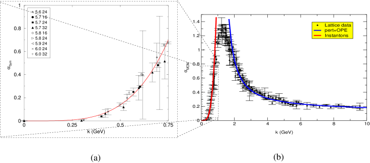
Figure 1: (b) Symmetric MOM coupling constant for different lattice settings and fits to perturbative expression plus power corrections in the high momenta region and to expression (14) discussed in the text for small momenta. (a) Region of small momenta is zoomed.

An important question arises here. How can we be sure that what we see are really instanton-like objects ? We have already noticed that the result in (14) is obtained for any radial profile of the semi-classical structures considered, provided the tensorial structure is that of eq. (6). But it is easy to see that any semi-classical field configuration different from eq. (6) would also produce a $p^{4}$ law but with a different prefactor. Therefore we might as well have seen other structures than instantons and thus our estimate of the density, which relies on the prefactor as compared to the one-instanton prediction, could be wrong.

In order to check our interpretation we appeal to cooled configurations. We insist that we do not use the controversial cooled configurations to infer the properties of the thermalised ones, but only to check our new method to estimate the instanton density against the instanton shape recognition (ISR) method which can only be applied after cooling. We cool the configurations according to the method described in [5] and compute the “strong coupling constant”  according to the scheme described section 2.1. The first striking result is that after cooling the coupling constant grows in the whole energy range (Figure 2). It reaches exceedingly large values at large momenta, the reason of which being the $\propto p^{4}$ law and the large prefactor due to a small instanton density, see eq. (14).

We now make a fit to a $p^{4}$ law for $\alpha_{\rm MOM}(p)$ on lattice configurations which have been submitted to a large number of cooling sweeps (200) so that UV fluctuations should have disappeared leaving only semiclassical structures. We do not take in the fit the few smallest momenta for reasons which will be discussed soon. We compare the instanton density extracted via formula (14) applied to the $\propto p^{4}$ fit of $\alpha_{\rm MOM}(p)$ to the instanton density coming from the geometrical “instanton shape recognition” (ISR) method described in [5]. We obtain the qualitative agreement shown in table 1. Notice that these values for the instanton densities have nothing to do with the latter density in the thermalised configuration . What is relevant is the fair agreement between both methods to estimate the instanton density.

L	$\beta$	n(ISR)	n($\alpha$)
24	5.6	0.009(6)	0.019(1)
24	5.8	0.048(23)	0.090(1)
24	6.0	0.115(6)	0.133(2)
32	6.0	0.145(16)	0.197(7)

Table 1: Comparison between the instanton density, n (in ${\rm fm}^{-4}$), obtained through the Instanton Shape Recognition (ISR) method [5] and the density deduced from the fit of the coupling constant after 200 cooling sweeps. In both cases errors are only statistical.

We expect differences in table 1 between both estimates, mainly at small $\beta$, because the ISR method does not recognize small instantons in lattice units, which induces for ISR a systematic underestimate of the density [28]. The general tendency in table 1 supports this argument, as both estimates of the density are closer for large values of beta .

In figure 2(a) it can be seen that at low momentum the points for $\alpha_{\rm MOM}$ are below the fit. The log-log plot of the same quantity for different cooling sweeps in figure 2(b) confirms that the behavior at small momenta differs slightly from the large momenta one. In fact the detailed dependence of the slopes in the momentum and the number of cooling sweeps seems to be involved but it is striking that the slope stays always in the range three to five, i.e. close to the expected slope four.

Anyhow, why do the thermal configuration seem to agree at small momentum with the $\propto p^{4}$ law, fig. 1(a), while the cooled configurations seem unexpectedly to agree with the same law only at larger momentum ? One might argue that at large distance instanton deformation [28] as well as instanton (anti-)instanton repulsion (attraction) might have been generated by the cooling itself . This would explain why the $p^{4}$ law observed at small momentum in the thermalised configurations tends to be distorted with cooling. Honestly this argument has to be submitted to closer scrutiny and for now we consider the detailed understanding of these slopes as an open question, but we would like to stress that anyhow the observed behaviour is never far from $\propto p^{4}$.

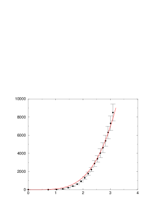
a	b

Figure 2: (a) Coupling constant in a cooled lattice ($L=24$,$\beta=6.0$) after 200 cooling sweeps. The solid line corresponds to the fit discussed in the text. The horizontal axis is given in GeV, assuming for simplicity the lattice spacing of the thermalised configurations, $a^{-1}=1.97$ GeV. (b) Coupling constant in a cooled lattice ($L=24$,$\beta=5.6$) after several cooling sweeps. The horizontal axis is the momentum assuming the same lattice spacing, $a^{-1}=0.83$ GeV, which is the value for the thermalised configurations. This is a log-log plot which exhibits better the power law. There seems to be three regimes.

4 Conclusion and discussion

• We have found that the lattice simulations indicate good scaling of $\alpha_{\rm MOM}(p)$ when the lattice spacing is varied, even at rather small $\beta$ when $p$ is small.

• We find

  $$\alpha_{\rm MOM}(p)\simeq\frac{1}{18\pi}n^{-1}p^{4},\quad{\rm for}\quad p\leq 0.8{\rm GeV}$$ (15)

  as expected from an instanton liquid picture and eq. (14).

• The fitted density

  $$n=5.27(4){\rm fm}^{-4}$$ (16)

  is in fair agreement with expectations.

• We have checked that the calculation of the instanton density from eq. (14) via a $\propto p^{4}$ fit of $\alpha_{\rm MOM}(p)$ is comparable to a direct counting of instantons recognised from their shape. We take this as a convincing evidence that this new $\alpha_{\rm MOM}$-method to measure instanton density is reliable.

This makes it highly plausible that this $\alpha_{\rm MOM}(p)\propto p^{4}$ is an effect of a liquid of instantons, i.e. that such a liquid of instantons indeed exists in the thermalised configurations and that the quantum fluctuations do not affect significantly $\alpha_{\rm MOM}(p)$ for  $p\leq 0.8$ GeV.

These results open a Pandora box of new questions: can this simple explanation also apply to other definitions of $\alpha_{s}$, to other Green functions (the gluon propagator in particular) ? How is this interpretation related to Schwinger-Dyson or renormalisation group deduced small momentum behavior of these quantities ?

A look at figure 1 (b) shows a nice theoretical understanding (solid lines) of $\alpha_{\rm MOM}(p)$ both in the large (perturbative QCD + OPE) and small (instanton liquid picture) momentum regimes. How to understand better the transition between these two regimes ?

5 Acknowledgments

We are grateful to Dmitri Shirkov for illuminating discussions. This work was supported in part by the European Network ”Hadron Phenomenology from Lattice QCD” HPRN-CT-2000-00145 and by Picasso agreement HF2000-0056. F.S. is indebted to the Spanish Fundación Cámara for financial support.

References

- [1] P. Boucaud et al., JHEP 0004, 006 (2000) [arXiv:hep-ph/0003020];
- [2] P. Boucaud, J. P. Leroy, J. Micheli, O. Pene and C. Roiesnel, JHEP 9810, 017 (1998) [arXiv:hep-ph/9810322]. D. Becirevic, P. Boucaud, J. P. Leroy, J. Micheli, O. Pene, J. Rodriguez-Quintero and C. Roiesnel, Phys. Rev. D 61, 114508 (2000) [arXiv:hep-ph/9910204]; Phys. Rev. D 59, 094509 (1999) [arXiv:hep-ph/9903364].
- [3] P. Boucaud, A. Le Yaouanc, J. P. Leroy, J. Micheli, O. Pene and J. Rodriguez-Quintero, Phys. Lett. B 493, 315 (2000) [arXiv:hep-ph/0008043]; F. De Soto and J. Rodriguez-Quintero, Phys. Rev. D 64, 114003 (2001) [arXiv:hep-ph/0105063].
- [4] P. Boucaud, A. Le Yaouanc, J. P. Leroy, J. Micheli, O. Pene and J. Rodriguez-Quintero, Phys. Rev. D 63, 114003 (2001), [arXiv:hep-ph/0101302].
- [5] P. Boucaud et al., Phys. Rev. D 66, 034504 (2002), [arXiv:hep-ph/0203119]; Talk given by J. Rodriguez-Quintero at 37th Rencontres de Moriond on QCD and Hadronic Interactions, Les Arcs, France, 16-23 Mar 2002, [arXiv:hep-ph/0205187]; P. Boucaud et al., Talk given by F. De Soto at 30th International Meeting on Fundamental Physics (IMFP 2002), Jaca, (Huesca), Spain, 28 Jan - 1 Feb 2002. arXiv:hep-ph/0210098.
- [6] D. V. Shirkov, arXiv:hep-ph/0208082; D. V. Shirkov, arXiv:hep-th/0210013.
- [7] J. Skullerud and A. Kizilersu, JHEP 0209, 013 (2002) [arXiv:hep-ph/0205318].
- [8] R. Alkofer and L. von Smekal, Phys. Rept. 353, 281 (2001) [arXiv:hep-ph/0007355].
- [9] B. Alles, D. Henty, H. Panagopoulos, C. Parrinello, C. Pittori, D.G. Richards, Nucl. Phys. B502 (1997) 325; C. Parrinello Nucl. Phys. Proc. Suppl. 63 (1998) 245; B. Alles, D. Henty, H. Panagopoulos, C. Parrinello, C. Pittori, IFUP-TH-23-96, hep-lat/9605033.
- [10] H. Nakajima and S. Furui, Presented at 20th International Symposium on Lattice Field Theory (LATTICE 2002), Boston, Massachusetts, 24-29 Jun 2002, [arXiv:hep-lat/0208074].
- [11] G. ’t Hooft, Phys. Rev. D 14 (1976) 3432 [Erratum-ibid. D 18 (1976) 2199].
- [12] T. Schafer and E. V. Shuryak, Rev. Mod. Phys. 70 (1998) 323.
- [13] D. Diakonov and V. Y. Petrov, Nucl. Phys. B 245 (1984) 259.
- [14] J. J. Verbaarschot, Nucl. Phys. B 362 (1991) 33 [Erratum-ibid. B 386 (1991) 236].
- [15] M. Hutter, arXiv:hep-ph/0107098.
- [16] M. Teper, Phys. Lett. B 162, 357 (1985); Phys. Lett. B 171 (1986) 86.
- [17] C. Michael and P. S. Spencer, Phys. Rev. D 52, 4691 (1995) [arXiv:hep-lat/9503018].
- [18] P. de Forcrand, M. Garcia Perez and I. O. Stamatescu, Nucl. Phys. B 499, 409 (1997) [arXiv:hep-lat/9701012].
- [19] D. A. Smith and M. J. Teper [UKQCD collaboration], Phys. Rev. D 58 (1998) 014505 [arXiv:hep-lat/9801008].
- [20] S. Bilson-Thompson, F. D. Bonnet, D. B. Leinweber and A. G. Williams, Nucl. Phys. Proc. Suppl. 109, 116 (2002) [arXiv:hep-lat/0112034].
- [21] M. Garcia Perez, O. Philipsen and I. O. Stamatescu, Nucl. Phys. B 551, 293 (1999) [arXiv:hep-lat/9812006].
- [22] A. Ringwald and F. Schrempp, Phys. Lett. B 459, 249 (1999) [arXiv:hep-lat/9903039].
- [23] I. Horvath et al., Phys. Rev. D 66, 034501 (2002) [arXiv:hep-lat/0201008].
- [24] I. Hip, T. Lippert, H. Neff, K. Schilling and W. Schroers, Phys. Rev. D 65, 014506 (2002) [arXiv:hep-lat/0105001].
- [25] J. B. Zhang, S. O. Bilson-Thompson, F. D. Bonnet, D. B. Leinweber, A. G. Williams and J. M. Zanotti, Nucl. Phys. Proc. Suppl. 109A (2002) 146.
- [26] J. W. Negele, Nucl. Phys. Proc. Suppl. 73, 92 (1999) [arXiv:hep-lat/9810053].
- [27] M. Guagnelli, R. Petronzio, J. Rolf, S. Sint, R. Sommer and U. Wolff [ALPHA Collaboration], Nucl. Phys. B 595, 44 (2001) [arXiv:hep-lat/0009021].
- [28] Ph. Boucaud et al., “Addendum to Instantons and condensate”, in preparation.