Angular Distribution of Particle Flows and Perturbative QCD Predictions

Abstract

We discuss the predictions of perturbative QCD for angular flows of final state particles in two and three jet events including their $cms$ energy and jet resolution ($y_{cut}$) dependence. The simple analytical formulae for gluon bremsstrahlung from primary partons, modified for gluon cascading, reproduce the main features of the experimental data well. For $y_{cut}$-selected events, the particle flow is derived from a superposition of colour dipoles in much the same way that photon radiation is derived from electric dipoles.

MPI-PhT/02-2002-78

IPPP/02/80; DCPT/02/160

1 Introduction

We study the angular distribution of particles between the hadronic jets in the final state of a high energy collision. The angular flow of such particles, most of them with low momentum $<1$ GeV, is expected to depend characteristically on the colour connections of the primary partons [1, 2, 3] (for recent reviews, see, for example, Ref. [4]). An early example of such a phenomenon concerns the final state $e^{+}e^{-}\rightarrow q\overline{q}g$. The soft radiation is not distributed symmetrically between the three jets, but rather is depleted in the angular region between the $q$ and $\overline{q}$ directions. This effect was first predicted within the string hadronization model [5]. Subsequently, it has been derived within perturbative QCD [6] where the particle flow is derived directly from the soft gluon bremsstrahlung, which is emitted coherently from all primary partons but with different strength from gluon and quark emitters according to the QCD colour factors.

The first observation of the effect was due to the JADE collaboration [7] with many of the subsequent details having been studied by various experimental groups, for example [8, 9, 10]. This “string/drag effect” is by now well established and reproduced by the popular Monte Carlo models. The analytic calculations have been verified mainly for angles midway between the jets. Until now, the full angular pattern predicted by perturbative QCD had not been compared systematically with data. At PEP energies the TPC collaboration [8] found that their data – though in qualitative agreement with QCD expectations – showed some quantitative differences with the asymptotic analytical results, which could have possibly been caused by the low purity of the quark/gluon identification of the jets. At LEP there has been considerable progress in jet identification, in particular by DELPHI [9]; their result for the “Mercedes configuration” has been compared successfully [4] with the analytic calculation [6, 11]. Comparison with the limited results by OPAL [10], averaged over a large range of jet angles, has been moderately successful.

In this paper we compare the experimental results for the various symmetric and asymmetric angular configurations of $q\bar{q}g$ presented by DELPHI and OPAL for the full angular region, along with the results for $q\bar{q}\gamma$ and two jet events with theoretical predictions. Furthermore, we discuss the energy and jet resolution dependence of the effect which has been ignored in the previous analyses.

2 Angular pattern of particle flows

2.1 Perturbative results and dependence on the jet selection

Let us begin by recalling the main ideas [6] in the perturbatively-based calculation of particle flows in $e^{+}e^{-}\rightarrow q\overline{q}g$ at high energies in comparison with $e^{+}e^{-}\rightarrow q\overline{q}\gamma$. We consider the configurations where all the angles $\Theta_{ij}$ between jets are large ($i=\{+-1\}\equiv\{q\overline{q}g\}$ or $i=\{+-\}\equiv\{q\overline{q}\}$). Within the perturbative picture, the angular distribution of soft inter-jet hadrons is calculated from the distribution of soft gluons radiated coherently off the colour antenna formed by the primary emitters $(q,\overline{q}$ and $g$) or $(q$ and $\overline{q})$.

The angular distribution of a secondary soft gluon, $g_{2}$, is derived in lowest order perturbation theory from the corresponding Feynman diagrams of single gluon emission off the primary partons. For the $q\bar{q}\gamma$ process one finds neglecting the recoil

$$\frac{8\pi dN_{q\overline{q}\gamma}}{d\Omega_{\vec{n_{2}}}E_{2}dE_{2}}=\frac{4C_{F}\alpha_{s}(k_{t})}{\pi}\;\frac{(p_{+}p_{-})}{(p_{+}k_{2})\;(p_{-}k_{2})}$$ (1)

with 4-momenta $p_{+},p_{-}$ and $k_{2}$ and soft gluon energy and transverse momentum $E_{2}$ and $k_{t}$.

A modification is necessary to take into account the fact that the “detected” gluon belongs to a parton jet. The results of the calculation for $q\overline{q}\gamma$ can be written as

$$\frac{8\pi dN_{q\overline{q}\gamma}}{d\Omega_{\vec{n_{2}}}}=\frac{1}{N_{C}}\;W_{+-}(\vec{n}_{2})\>N_{g}^{\prime}(Y)\;=\;\frac{2C_{F}}{N_{C}}\;(\widehat{+-})\>N_{g}^{\prime}(Y),$$ (2)

and for $q\overline{q}g$ one finds

$$\frac{8\pi dN_{q\overline{q}g}}{d\Omega_{\vec{n}_{2}}}=\frac{1}{N_{C}}\;W_{\pm 1}\>(\vec{n}_{2})\>N_{g}^{\prime}(Y)\;=\;\left[(\widehat{1+})+(\widehat{1-})\>-\>\frac{1}{N_{C}^{2}}\;(\widehat{+-})\right]\;N_{g}^{\prime}(Y).$$ (3)

Here the angular distribution of soft gluon bremsstrahlung from the “antenna”-dipole $(\widehat{ij})$ is obtained from (1) and reads

$$(\widehat{ij})\;=\;\frac{a_{ij}}{a_{i}a_{j}},\;\;\;\;a_{ij}\;=\;(1\>-\>\vec{n}_{i}\vec{n}_{j}),\;\;\;\;a_{i}\;=\;(1\>-\>\vec{n}_{2}\vec{n}_{i}).$$ (4)

This angular distribution is the same as that for photon bremsstrahlung in QED – as it occurs, for example, in $e^{+}e^{-}$ pair creation. Unlike the QED case, however, there are also the QCD-specific colour factors and the “cascading factor” $N_{g}^{\prime}(Y)$, which takes into account the fact that $g_{2}$ is part of a jet. It represents the derivative of particle multiplicity in a gluon jet with respect to $Y=\ln(K_{T}/Q_{0})$ at the appropriate maximal transverse momentum scale $K_{T}$ and cut-off $Q_{0}$. The parameter $Q_{0}$ is determined from a fit to the multiplicity data together with the QCD scale $\Lambda$ ($Q_{0}\mathrel{\mathop{\kern 0.0pt\hbox to0.0pt{\raise 0.86108pt\hbox{$>$}\hss}}\lower 3.87495pt\hbox{\kern-1.90002pt$\sim$}}\Lambda$, see, for example [4]).

The scale $K_{T}$ depends on the way the jets are selected. To see this, we write down the perturbative expansion for the emission of gluon $g_{2}$ in (2) from the primary parton $p$ as follows (see also [12])

$$\begin{split}\frac{8\pi dN_{q\overline{q}\gamma}}{d\Omega_{\vec{n_{2}}}}&=\frac{1}{N_{C}}\;\int^{E_{max}}_{E_{min}}\frac{dE_{2}}{E_{2}}W_{+-}({\vec{n_{2}}})\gamma_{0}^{2}(k^{t}_{2p})\\ &\quad+\frac{1}{N_{C}}\;\int^{E_{max}}_{E_{min}}\frac{dE_{2}}{E_{2}}\int^{E_{max}}_{E_{2}}\frac{dE_{a}}{E_{a}}\int\frac{d\Omega_{ap}}{2\pi\Theta_{ap}^{2}}\gamma_{0}^{2}(k^{t}_{ap})W_{+-}({\vec{n_{a}}})\gamma_{0}^{2}(k^{t}_{2a})+\ldots\\ &\approx\frac{1}{N_{C}}\;W_{+-}({\vec{n_{2}}})\int^{E_{max}}_{E_{min}}\frac{dE_{a}}{E_{a}}\gamma_{0}^{2}(k^{t}_{2p})[1+\int^{E_{a}}_{E_{min}}\frac{dE_{2}}{E_{2}}\int\frac{d\Omega_{a2}}{2\pi\Theta_{a2}^{2}}\gamma_{0}^{2}(k^{t}_{a2})+\ldots].\end{split}$$ (5)

The first term corresponds to the Born result for direct gluon emission in (1), the second one to the emission through the intermediate parton $a$. We denote by $k^{t}_{ab}$ and $\Theta_{ab}$ the transverse momentum and angle respectively of parton $a$ with respect to parton $b$, in addition $\Theta_{ap}\equiv\Theta_{a}$; the leading order multiplicity anomalous dimension is given by $\gamma_{0}^{2}(k_{t})=2N_{C}\alpha_{s}(k_{t})/\pi$. Eq. (5) is written in DLA, but it can also be generalized to MLLA after inserting the appropriate splitting functions in all intermediate branchings.

In the second equation in (5) we have replaced the integral over the angle $\Theta_{ap}$ by the integral over $\Theta_{a2}$, as the leading contribution to the $a$ integral comes from the region of quasi-collinear emission $\vec{n_{a}}\simeq\vec{n_{2}}$; then we also replace the corresponding angles involving particle $a$ in $W_{+-}$. Furthermore, the order of integration between $E_{a}$ and $E_{2}$ is interchanged ($E_{2}<E_{a}$). Now, the angular integral in the second term has to satisfy the “angular ordering” requirement, i.e. the emission angle of the intermediate parton $a$ should respect

$$\Theta_{2a}<\Theta_{ap};\quad\text{therefore, also}\quad\Theta_{ap}>\Theta_{2p}/2.$$ (6)

Then the angular integral can be performed with $\Theta_{a2}<\Theta_{2}$ in pole approximation.

Next we discuss the limits of the energy integrations in (5). The lower limit $E_{min}$ is determined by the transverse momentum cut-off. For gluon emission inside a well separated jet one requires $k_{t}>Q_{0}$, therefore $E_{min}\approx Q_{0}/\Theta_{2}$ in the small angle approximation. In case of emission from a boosted $q\overline{q}$ “dipole” as in (1) an azimuthal dependence of the effective cut-off $Q_{0}$ around the jet axis is generated. To estimate this effect we consider a generalization of the cut-off restriction following from (1)

$$\tilde{k}_{t}^{2}=\frac{2(p_{+}k)(p_{-}k)}{p_{+}p_{-}}=\frac{2E_{2}^{2}(1-\cos\Theta_{+2})(1-\cos\Theta_{-2})}{1-\cos\Theta_{+-}}\ >\ Q_{0}^{2},$$ (7)

which approaches the limit $\tilde{k}_{t}=k_{t}$ for the $q\overline{q}$ back-to-back configuration. For our applications the effective $k_{t}$ cut-off $Q_{0}$ will then change by up to a factor 2. In the asymptotic expansion of multiplicity [14, 2] $\ln N_{g}(Y)=c_{1}\sqrt{Y}+c_{2}\ln Y+c_{3}/\sqrt{Y}$ such a rescaling $Q_{0}\to\beta Q_{0}$ would modify only the $c_{3}$ term, therefore the leading (DLA) and next-to-leading (MLLA) results remain unchanged. Numerically, for the present analysis we estimate the effect on $N^{\prime}$ in (2),(3) from the variation of $Q_{0}$ to be at the 10-20% level where we take into account the data in Fig. 4a below. In our application of analytic high energy approximations (large $K_{T}/Q_{0}$) we continue therefore with the cut-off $k_{t}>Q_{0}$ in the following.

The upper limit $E_{max}$ of the energy integral depends on the jet selection procedure and we consider two cases
a) no momentum restriction in jet selection
In the simplest case, we require 2 or 3 respectively energetic particles in the given angular directions which define the jet directions. A more precise definition is possible using the energy-energy-multiplicity or energy-energy-energy-multiplicity correlations for 2 and 3 jets [15, 3]. For two jets one considers all pairs of particles (ij) weighted with their energies, and for a given relative angle $\Theta_{ij}$, one studies the angular distribution of all soft particles in the event. In the same way one proceeds for 3-jet events with triples of energy weighted particles and two relative angles.

In these cases there is no specific restriction on the energy of the triggered soft particles whose angular distribution is investigated. The maximum energy $E_{max}$ of these particles is then of order of the respective jet energies $E_{jet}$, say $\sqrt{s}/2$ or $\sqrt{s}/3$ in 2 and 3 jet events at total cms energy $\sqrt{s}$ of the jet system, and the same applies to the intermediate partons $a$.

b) selection of jets for a given resolution parameter $y_{cut}$
We consider here the “Durham algorithm” [16] which selects the jets according to a predefined minimal relative transverse momentum, approximately $K_{T}\geq\sqrt{y_{cut}s}$. In this case, the $y_{cut}$ selection restricts the transverse momenta of emitted particles $g_{2}$ as well as the transverse momenta of the intermediate partons $a$ in (5) in the same way ($k^{t}_{ap}<K_{T}$), whereas the longitudinal momenta of the latter partons $a$ are only limited by ${\cal O}(\sqrt{s})$. However, an additional restriction comes from the angular ordering (6), which is violated for intermediate partons $a$ with large energies and, thus, small angles $\Theta_{ap}$. In our logarithmic approximation we take the same upper limit for the $E_{a}$ and $E_{2}$ integrals. Similarly, the angular integral is limited by $\Theta_{a2}<\Theta_{2}$ within the same accuracy. Then, the second equation in (5) can be resummed, resulting in the multiplicity $N_{g}(K_{T}/Q_{0})$

$$\frac{8\pi dN_{q\overline{q}\gamma}}{d\Omega_{\vec{n_{2}}}}\approx\frac{1}{N_{C}}\;W_{+-}({\vec{n_{2}}})\int^{E_{max}}_{E_{min}}\frac{dE_{2}}{E_{2}}\gamma_{0}^{2}(k^{t}_{2p})N_{g}(k^{t}_{2p}/Q_{0}).$$ (8)

This integral can be expressed in terms of $N^{\prime}(Y)$ using the evolution equation for multiplicity, which then leads to Eq. (2). We note that this replacement is also possible in MLLA.

The upper limit of integration $E_{max}$ is either given by the maximal energy $E_{jet}$ of the jet or depends on the jet resolution parameter $y_{cut}$

case a (no restriction) $$Y=\ln(E_{jet}\Theta_{m}/Q_{0})$$ (9)

$$\text{case b ($y_{cut}$ restriction}) Y=\begin{cases}\ln(E_{jet}\Theta_{m}/Q_{0})&\Theta_{m}<\sqrt{y_{cut}s}/E_{jet}\\ \ln(\sqrt{y_{cut}s}/Q_{0})&\text{otherwise}\end{cases}$$ (10)

Here $\Theta_{m}$ is the angle between the soft gluon $g_{2}$ and the jet closest in angle. As the multiplicity $N_{g}$ depends on the maximum transverse momentum scale, the Durham $K_{T}$ - algorithm naturally provides simple results. Note that in case of $y_{cut}$ selection (case b), the $N^{\prime}(Y)$ factor becomes independent on the emission angle $\Theta_{m}$ away from the jet directions, and, therefore, the soft gluon angular distribution is given simply by the Born-term factors $W(\vec{n_{2}})$ in (2,3).

2.2 Projection onto the event plane

We are now interested in the projection of the soft gluon $g_{2}$ angular distribution onto the event plane defined by the momentum vectors of the $q\bar{q}g(\gamma)$ systems. The azimuthal angle $\phi$ in the plane is defined to be zero in the direction of $q$, becoming positive in the direction of $\bar{q}$ for definiteness (in our applications $q$ and $\bar{q}$ are not distinguishable), see Fig. 1. The projection of the particle density onto the event plane is obtained in the case of $q\overline{q}\gamma$ from the integral over $\cos\Theta_{2}$, where $\Theta_{2}$ is the polar angle with respect to the normal to the event plane,

$$W_{+-}(\phi) = 2C_{F}\;\int\;\frac{d\cos\Theta_{2}}{2}\;(\widehat{+-})\;=\;2C_{F}\>a_{+-}\>V(\alpha,\beta),$$ (11)

$$V(\alpha,\beta) = \frac{2}{\cos\alpha-\cos\beta}\>\left(\frac{\pi-\alpha}{\sin\alpha}\>-\>\frac{\pi-\beta}{\sin\beta}\right),$$

the angles $\alpha,\beta$ are given below in terms of $\phi$.

Replacing $\gamma$ by the hard gluon $g_{1}$ one obtains an additional particle flow in the $g_{1}$ direction, and from the integration of Eq. (3) over cos$\Theta_{2}$ one derives

$$W_{\pm 1}(\phi)=N_{C}\>\left[a_{+1}V(\alpha,\gamma)+a_{-1}V(\beta,\gamma)-\frac{1}{N_{C}^{2}}\>a_{+-}V(\alpha,\beta)\right].$$ (12)

For an arbitrary choice of $\phi$ the angles $\alpha,\beta,\gamma$ in the projection formulae (11),(12) have to be defined as minimal angles between the directions of the soft gluon ($g_{2}$) and the directions of $q,\bar{q}$ and $g$ respectively, with all angles within the interval $[0,\pi]$. We find the following definition of the angles $\alpha,\beta,\gamma$ to satisfy this requirement and to apply in all angular sectors with $\phi$ running from $0$ to $2\pi$ (see also Fig. 1)

$$\alpha = \min(\phi,2\pi-\phi);\quad\beta=\min(|\Theta_{+-}-\phi|,2\pi-\phi+\Theta_{+-});$$ (13)

$$\gamma = \min(\phi+\Theta_{1+},|2\pi-\Theta_{1+}-\phi|).$$ (14)

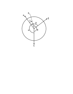
Figure 1: Definition of azimuthal angles in the event plane of three jet event.

Eq. (12) corresponds to an incoherent superposition of two Lorentz-boosted dipoles, one between the gluon and the quark and one between the gluon and the anti-quark, modified by the negative correction of ${\cal O}(1/N_{c}^{2})$. This expression shows a depletion opposite to the gluon direction.

2.3 Comparison with experiment

Let us now compare these analytical formulae with experimental data. The DELPHI collaboration [9] has presented results on three jet events with two identified $b$-quark jets allowing for a high gluon jet purity ($\sim 94\%$). Symmetric angular configurations have been selected – either “Mercedes” or “Y-symmetric” events with angles confined to an angular region of $\pm 15^{\circ}$. Furthermore, the data on the final state $q\bar{q}\gamma$ in the Y-configuration have been presented. These well defined event classes are compared in Fig. 2 with the above analytical formulae.

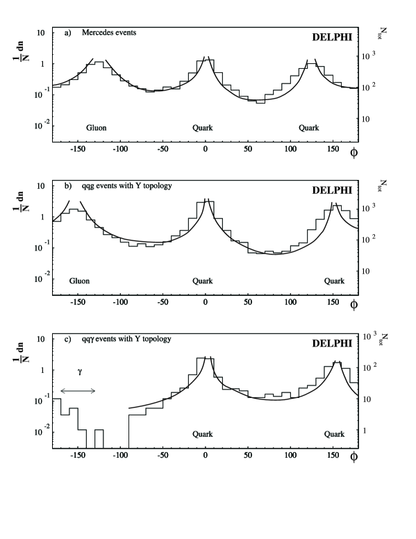
Figure 2: Charged particle flow within various multi-jet configurations as measured by DELPHI [9] (a) “Mercedes” $q\bar{q}g$ events, (b) “Y-symmetric” $q\bar{q}g$ events and c) $q\bar{q}\gamma$ events, in comparison with analytical QCD predictions; the curves correspond to the lowest order QCD soft bremsstrahlung formulae. The relative angles between the jets are taken in a) as $\Theta_{1+}=125^{\circ}$, $\Theta_{+-}=122.5^{\circ}$ and $\Theta_{1-}=112.5^{\circ}$; in b) and c) as $\Theta_{+-}=\Theta_{1+}=150^{\circ}$.

The angle $\phi=0$ is in the direction of the most energetic quark jet. For Mercedes events, we chose the other jet angles at the observed peak positions – slightly different ($<8^{\circ}$) from the symmetric values. The events had been selected with fixed $y_{cut}\simeq 0.01$ according to the Durham algorithm. As a result, we can neglect the variation of the cascading factor $N_{g}^{\prime}$ in (2) and (3) (for angles $\mathrel{\mathop{\kern 0.0pt\hbox to0.0pt{\raise 0.86108pt\hbox{$>$}\hss}}\lower 3.87495pt\hbox{\kern-1.90002pt$\sim$}}20^{\circ}$ away from the jet directions). The shape of the angular distribution is then predicted without a free parameter; in Fig. 2 only one overall normalization factor has been fitted in the description of the three distributions.

The general characteristics of the distributions are well reproduced, in particular the different heights of the inter-jet valleys. In addition, the larger width of the gluon jet in comparison with the central quark jet width becomes visible. The quark-jets in a) and b) are a bit broader than perturbatively predicted, as can be expected from the b-quark jet selection; the quark-jets at the larger angle $\phi$ in a) and b) are even broader because of the angular fluctuation in the selection of the jets. This successfull description nicely demonstrates the similarity of particle flow in “strong interaction” processes to photon flow in electromagnetic interactions – both are caused by the underlying gauge boson bremsstrahlung in QED and QCD. In c) the formulae are equivalent, in a) and b) they are modified by the different colour charges for quarks and gluons – a degree of freedom not available in QED. An interesting QCD interference effect is the negative $1/N_{C}^{2}$ term in (3). Unfortunately, according to our analysis, the presented data are not sufficient for a reliable observation of this term.

A comparison of $q\bar{q}g$ and $q\bar{q}\gamma$ distributions between the quark and anti-quark jets has been presented by OPAL [10]. In the analysis of $q\bar{q}g$ events, the jets are ordered according to their energies. The jet with the lowest energy in the $q\bar{q}g$ system is taken as the gluon jet and two intervals of this energy $E_{3}$ are selected around $E_{3}=10$ and $E_{3}=20$ GeV, furthermore, $\Theta_{+-}\simeq 165^{\circ}$ from which we can estimate $\Theta_{1-}$ and $\Theta_{1+}$. In the calculation we take into account the estimated purities of gluon jets, $p_{g}$, by superimposing the distribution (2) with the one obtained by swapping the second and third jet, i.e. by swapping $\Theta_{+-}$ and $\Theta_{1+}$ and changing $\phi$ to $2\pi-\phi$. The original distribution gets the weight $p_{g}=0.92$ for the sample with $E_{3}=10$ and $p_{g}=0.74$ for $E_{3}=20$ GeV, according to the reported purities.

In Fig. 3 we show the distribution in the rescaled azimuthal angle $X=\phi/\Theta_{+-}$ for the two processes as well as for their ratios in the two intervals of $E_{3}$. The different heights of both distributions near $X\simeq 0.5$ is rather well reproduced, as is the variation with energy $E_{3}$ and jet angle $\Theta_{1-}$. In particular, there is a sizeable asymmetry in the distribution which would be even more pronounced if the gluon jets were identified with higher purity. Since the data in both intervals still average a sizable range of different angular configurations, some deviations from the predictions are to be expected. We therefore allowed an increase of relative normalization by 15% of the curves in Fig 3 b) over Fig 3 a) to improve the description. The predictions are seen to fall below the data for $dn/dX$ near the jet directions, which may be due to the averaging over the jets with different energies and angular widths. On the other hand, the difference in the splitting of the two distributions, in their asymmetry, and in their absolute height for the two angular configurations in a) and b) are well reproduced. The effects related to configuration asymmetry have been studied here for the first time; these effects could be investigated more precisely in the future if smaller intervals in the relative jet angles were chosen.

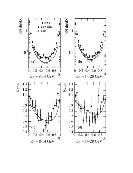
Figure 3: Charged particle flow in between the two quark jets of the $q\bar{q}g$ and $q\bar{q}\gamma$ final states, as measured by OPAL [10], for two samples of energies $E_{3}$ of the lowest momentum jet together with the corresponding ratios. The curves represent the lowest order QCD bremsstrahlung formulae for two intervals of the lowest energy $E_{3}$ of the jets; the overall normalization has been adjusted; in addition, the curves in b) are increased by 15% (see text). In our calculations we use for the first interval $E_{3}=10$ GeV, $\Theta_{+-}=165^{\circ}$, $\Theta_{1-}=67^{\circ}$ and $\Theta_{1+}=128^{\circ}$, and for the second one $E_{3}=20$ GeV, $\Theta_{+-}=165^{\circ}$, $\Theta_{1-}=35^{\circ}$ and $\Theta_{1+}=160^{\circ}$.

3 Energy dependence of particle angular flow

The energy ($\sqrt{s}$) and $y_{cut}$ dependences are determined by the cascading factor $N^{\prime}(Y)$ according to (9),(10). Angular distributions for particles produced in the hemispheres of quark and gluon jets without $y_{cut}$ restriction are available at different energies from $e^{+}e^{-}\to q\bar{q}$ and at LEP-1 energy from $e^{+}e^{-}\to b\bar{b}g$. Instead of the distribution in angle $\Theta$ we may also study the distribution in pseudo-rapidity $y=-\ln\tan(\Theta/2)$. For quark and gluon jets ($A=q,g)$ we have

$$\frac{dn_{A}}{dy}(E_{jet},y)=N^{\prime}_{A}(Y),\quad Y=\ln\left(\frac{E_{jet}\Theta}{Q_{0}}\right).$$ (15)

This relation is not limited to the leading order result $N_{q}/N_{g}=C_{F}/C_{A}$ as in Eq. (2) but allows for higher order logarithmic effects. Relation (15) follows from the MLLA result that the multiplicity depends only on the maximum $K_{T}$ in the jet, i.e. on the product $E_{jet}\Theta$ in the small angle approximation. Then, the variation of multiplicity with $y\simeq-\ln(\Theta/2)$ is the same as the one with $\ln E_{jet}\simeq y_{max}=\ln(2E_{jet}/m)$ or, equivalently, the particle density depends on rapidity and energy only through the scaling variable

$$x=y-\ln(\sqrt{s}/\mu)\ =\ -\ln(E_{jet}\Theta/\mu)$$ (16)

where we set $\mu=1$ GeV and $\sqrt{s}=2E_{jet}$. Eq. (15) predicts both the energy dependence at fixed angle (rapidity) and the angular dependence at fixed energy. Recall that within the MLLA approach [2, 11] the multiplicity $N$ depends only on the phenomenological parameter $Q_{0}\sim\Lambda$ and a normalization factor, then the angular distribution is uniquely predicted by (15).

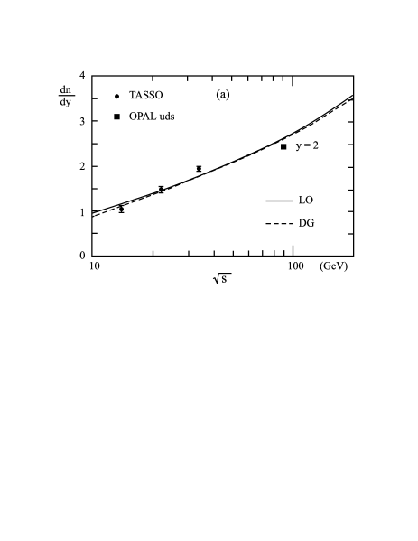
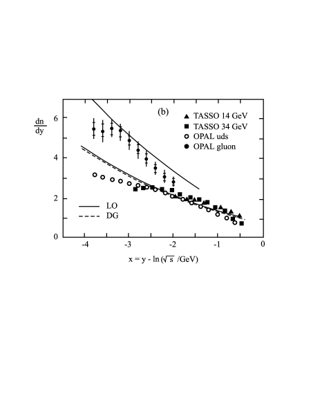
Figure 4: Distribution in rapidity $y$ (a) at fixed rapidity $y=2$ versus energy $\sqrt{s}$ and (b) as a function of the shifted rapidity $x=y-\ln(\sqrt{s}/{\rm GeV})$ at different energies $\sqrt{s}$ (assuming pion mass for all charged particles), in comparison with solutions of the MLLA evolution equations for $N^{\prime}$ by Dremin and Gary (DG) [18] and by Lupia and Ochs (LO) [19]; data by TASSO [20] and OPAL [21].

These predictions have been tested by comparing the QCD results for $N^{\prime}_{A}$ with data from TASSO and OPAL (here from $uds$-quark jets only to avoid the heavy-quark contribution at the $Z$ mass) in Fig. 4. The curves in Fig. 4 represent the high energy QCD 3NLO prediction (DG [18]) and the numerical solution (LO [19]) of the full MLLA evolution equations for quark and gluon jets [11] . In both calculations the parameters have been determined from a fit to $e^{+}e^{-}$ data, and the two results agree for quark jets within $\sim 3\%$ in the energy region considered ($10<\sqrt{s}<200$ GeV). The data in Fig. 4a show the predicted increase with energy. In Fig. 4b we show the comparison for the rapidity distributions at different energies using the scaling variable $x$ in (16). At each energy, the lower bound of the rapidity interval is $y=0.8$. Above this value the scaling property is approximately satisfied, and, again, a good description by the theoretical calculation of $N^{\prime}(y)$ is obtained in absolute terms. However, some discrepency at low $y$ is seen for the OPAL data. Approximate agreement is also obtained with the distribution in gluon jets from OPAL [21] in the given rapidity range. For larger rapidities, the distibution would fall below the distribution for quarks as one may expect from energy conservation and recoil effects given the increased central production of particles. The curve shown corresponds to the common solution of the evolution equations for quark and gluon jets (LO [19]); the solution DG [18] with the quark jet parameters would result in a prediction larger by 20%; with readjusted parameters a good description is obtained again.

We conclude that the energy dependence of the angular distribution, given by $N^{\prime}(Y)$ in absolute terms, is reasonably well reproduced. A further improvement would require the treatment of (i) large angle and recoil corrections, (ii) dependence on jet axis definition (iii) heavy quark contribution and hadron mass effects.

The energy dependent effects discussed here are also expected in multi-jet events as in Eqs. (2, 3). Different analysis methods and configurations selected by different groups do not allow a meaningful comparison yet. Another interesting test will be the dependence of angular distributions on the jet resolution parameter $y_{cut}$ in (10).

4 Conclusion

The angular distribution of particles in two and three jet events follows closely the expectations based on the lowest order bremsstrahlung formulae of QCD. These formulae can be represented as sums over dipole radiation terms (4), the same as in QED, modified by the proper colour factors for quarks and gluons. In addition, there is an effect of parton branching which modifies these formulae by the “cascading factor” $N^{\prime}(Y)$, the logarithmic derivative of the multiplicity. For fixed resolution parameter $y_{cut}$, this factor does not modify the basic angular distribution in a wide range. On the other hand, it implies an additional dependence on energy and/or jet resolution. The predicted dependence on $N^{\prime}$ has been clearly established for two-jet events. These results demonstrate that soft multi-hadron production follows the simple expectations of perturbative QCD bremsstrahlung and confirm the close connection between the colour flows and observable flows of hadrons.

References

- [1] A. Bassetto, M. Ciafaloni and G. Marchesini, Phys. Rep. 100 (1983) 201.
- [2] Ya.I. Azimov, Yu.L. Dokshitzer,V.A. Khoze and S.I. Troyan, Z.Phys. C27 (1985) 65; ibid. C31 (1986) 213.
- [3] Yu.L. Dokshitzer, V.A. Khoze, S.I. Troyan and A.H. Mueller, Rev. Mod. Phys. 60 (1988) 373.
- [4] V.A. Khoze and W. Ochs, Int. J. Mod. Phys. A12 (1997) 2949; V.A. Khoze, W. Ochs and J. Wosiek, “At the frontier of particle physics – Handbook of QCD”, ed. M. Shifman, World Scientific (Singapore, 2001), Vol.2, p. 1101 (arXiv:hep-ph/0009298).
- [5] B. Andersson, G. Gustafson and T. Sjöstrand, Phys. Lett. 94B (1980) 211.
- [6] Ya.I. Azimov, Yu.L. Dokshitzer, V.A. Khoze and S.I. Troyan, Phys. Lett. 165B (1985) 147; Sov. J. Nucl. Phys. 43 (1986) 95.
- [7] JADE Collaboration: W. Bartel et al., Phys. Lett. B101 (1981) 129; Phys. Lett. B134 (1984) 275.
- [8] TPC Collaboration: H. Aihara et al., Phys. Rev. Lett. 57 (1986) 945.
- [9] DELPHI Collaboration: P. Abreu et al., Z. Phys. C70 (1996) 179.
- [10] OPAL Collaboration: R. Akers et al., Z. Phys. C68 (1995) 531.
- [11] Yu.L. Dokshitzer, V.A. Khoze, A.H. Mueller and S.I. Troyan, “Basics of Perturbative QCD”, ed. J. Tran Thanh Van, Editions Frontiéres, Gif-sur-Yvette, 1991.
- [12] Yu.L. Dokshitzer, G. Marchesini and G. Oriani, Nucl. Phys. B387 (1992) 675.
- [13] W. Ochs and J. Wosiek, Z. Phys. C68 (1995) 269.
- [14] B.R. Webber, Phys. Lett. B143 (1984) 501.
- [15] Yu.L. Dokshitzer, V.A. Khoze and S.I. Troyan, Sov. Journ. Nucl. Phys. 47 (1988) 881.
- [16] N. Brown and W.J. Stirling, Phys. Lett. B252 (1990) 657; Z. Phys. C53 (1992) 629; S. Catani, Yu.L. Dokshitzer, M. Olsson, G. Turnock and B.R. Webber, Phys. Lett. B269 (1991) 432.
- [17] CDF Collaboration: D.Acosta et al., FERMILAB-PUB-02-096E; Phys. Rev. D to be publ.; T. Affolder et al., Phys. Rev. Lett. 87 (2001) 211804.
- [18] I.M. Dremin and J.W. Gary, Phys. Lett. B459 (1999) 341; Phys. Rep. 349 (2001) 301.
- [19] S. Lupia and W. Ochs, Phys. Lett. B418 (1998) 214.
- [20] TASSO Collaboration: Z. Phys. C22 (1984) 307.
- [21] OPAL Collaboration: R. Akers et al., Eur. Phys. J. C11 (1999) 217.
- [22] ALEPH Collaboration: R. Barate et al., Phys. Rep. 294 (1998) 1.