UCB-PTH-02/59

SLAC-PUB-9612

hep-ph/0212180

Atmospheric Neutrinos Can Make Beauty Strange

Roni Harnik, Daniel T. Larson and Hitoshi Murayama

Theoretical Physics Group
Ernest Orlando Lawrence Berkeley National Laboratory
University of California, Berkeley, California 94720, USA

Department of Physics, University of California
Berkeley, California 94720, USA

Aaron Pierce

Theoretical Physics Group
Stanford Linear Accelerator Center
Stanford University, Stanford, California,94309, USA

The large observed mixing angle in atmospheric neutrinos, coupled with Grand Unification, motivates the search for a large mixing between right-handed strange and bottom squarks. Such mixing does not appear in the standard CKM phenomenology, but may induce significant $b\to s$ transitions through gluino diagrams. Working in the mass eigenbasis, we show quantitatively that an $\mathcal{O}(1)$ effect on CP violation in $B_{d}^{0}\to\phi K_{S}$ is possible due to a large mixing between $\tilde{s}_{R}$ and $\tilde{b}_{R}$, while still satisfying constraints from $b\to s\gamma$. We also include the effect of $\tilde{b}_{L}$-$\tilde{b}_{R}$ mixing proportional to $m_{b}\mu\tan\beta$. In the case where $m_{b}\mu\tan\beta\ll M^{2}_{SUSY}$ there may be a large effect in $B_{s}$ mixing correlated with a large effect in $B_{d}^{0}\rightarrow\phi K_{S}$, typically yielding an unambiguous signal of new physics at Tevatron Run II.

1 Introduction

Flavor physics has seen tremendous progress in the past few years. The discovery of neutrino oscillations by the SuperKamiokande [1], SNO [2] , and KamLAND [3] experiments clearly marks a historic event, while CP violation has recently been found in two new manifestations: direct CP violation in the neutral kaon system [4] and indirect CP violation in the the $B_{d}^{0}$ system [5]. On the other hand, we still lack insight into the origin of flavor and the patterns of masses and mixings. We need to look for any possible hints of physics that give us additional insight into these questions.

One of the major surprises in neutrino physics was the observation of (two) large angles. Unlike in the quark sector where all mixing angles in the Cabibbo–Kobayashi–Maskawa (CKM) matrix are small, both atmospheric and solar neutrino oscillations require large angles. An important question is whether the presence of large angles will give us new insight into the origin of flavor, masses, and mixings.

It was pointed out in Ref. [6] that the large angles in the neutrino sector may imply large angles in the mixing among right-handed down-type quarks if they are grand-unified with lepton doublets. Indeed, some $SO(10)$ models with Pati–Salam type unification of Yukawa matrices suggest that the large mixing angles in neutrinos arise from the charged lepton mass matrices, and thus also appear in the down-quark mass matrices. In these models, one assumes that these new large mixing angles do not appear in the CKM matrix because the right-handed charged-current interaction is broken at the Pati-Salam unification scale. However, the imprint of the large atmospheric neutrino mixing angle may appear in the squark mass matrices as a large $\tilde{b}_{R}$-$\tilde{s}_{R}$ mixing effect though radiative corrections due to the large top Yukawa coupling. The large solar neutrino mixing angle, however, does not cause a significant effect because of the smaller Yukawa coupling for lower generations. The new $\tilde{b}_{R}$-$\tilde{s}_{R}$ mixing in turn feeds into new effects in $B$-physics. In particular, there may be large new CP-violating effects in $b\rightarrow s$ transitions and enhanced $B_{s}$ mixing. It has already been noted that CP violation in $B_{d}^{0}\to\phi K_{S}$ is a good place to look for new physics effects [7, 8].

The time-dependent asymmetry in $B_{d}^{0}(\overline{B}_{d}^{0})\rightarrow\phi K_{S}$ was reported recently by both BaBar and BELLE. Their measurements differ from the value in the $J/\psi K_{S}$ final state by $\mathcal{O}(1)$. The standard model predicts that these two channels should give the same value. The significance of the difference is $2.7\sigma$ if the measurements from both collaborations are combined– the current world average for $\sin 2\beta$ in the $B_{d}^{0}\to J/\psi K_{S}$ channel is $0.734\pm 0.054$, while in the $B_{d}^{0}\to\phi K_{S}$ channel $S_{\phi K}=-0.39\pm 0.41$ [9]. This report has already sparked many speculations [10]. It is not clear if this is a temporary anomaly or a genuine new effect. Nonetheless it is important to study how large the new CP violation in $B_{d}^{0}\to\phi K_{S}$ can be and how it is correlated to $B_{s}$ mixing which will be studied soon at Tevatron Run II.

In this paper, we investigate the size of CP violation in $B_{d}^{0}\rightarrow\phi K_{S}$ as well as $B_{s}$ mixing from a potentially large $\tilde{b}_{R}$-$\tilde{s}_{R}$ mixing. There have also been several investigations of $B_{d}^{0}\rightarrow\phi K_{S}$ within the context of supersymmetry (SUSY) [8, 11, 12]. Of the above, only Ref. [12] investigated the correlation between the measurement of $\sin 2\beta$ in $B_{d}^{0}\rightarrow\phi K_{S}$ and $B_{s}$ mixing. However it uses the mass insertion formalism, which is not necessarily appropriate for the large mixing that we will consider. In addition, it appeared before the recent experimental results, and so it did not seek to reproduce such a large shift in $\sin 2\beta$. We perform a calculation in the mass eigenbasis, with a goal of determining whether supersymmetry can accommodate the central value of the recent experimental results for $\sin 2\beta$ in $B_{d}^{0}\to\phi K_{S}$. We then explore the consequences for $B_{s}$ mixing.

We also emphasize contributions to $\sin 2\beta$ that arise from a combination of $\tilde{b}_{L}$-$\tilde{b}_{R}$ ($m_{b}\mu\tan\beta$) and $\tilde{b}_{R}$-$\tilde{s}_{R}$ mixing. These contributions, which we find to be important over a wide region of parameter space, are not easily analyzed in the mass insertion approximation. Analogous combinations were studied in the kaon system [13], but to our knowledge these contributions have not been thoroughly analyzed with regard to new physics in the $B_{d}^{0}$ system.

The outline of the paper is as follows. In the next section we introduce the effective field theory formalism for $b$ decay and work out $b\rightarrow s$ transitions. In Section 3 we discuss $B_{s}$ mixing from large $\tilde{b}_{R}$-$\tilde{s}_{R}$ mixing. Section 4 is devoted to the discussion of correlations between the $b\rightarrow s$ transition and $B_{s}$ mixing. We conclude in Section 5. Details of some calculations are presented in the appendices. In Appendix A we show the loop functions, while the hadronic matrix elements are estimated in Appendix B.

2 CP Violation in $b\rightarrow s$ Transition

In this section we briefly review the well-known effective field theory formalism for $B$-physics (for a comprehensive review see  [14]), which we use to calculate the contribution of supersymmetric particles to $b\rightarrow s$ transitions. Using this machinery we discuss the contribution of a large mixing between right-handed squarks to the CP-violating parameter $S_{\phi K}$. We also use this formalism to address the constraints on the SUSY contribution that come from the $b\rightarrow s\gamma$ radiative decay.

2.1 Effective Hamiltonian

The $b\rightarrow s$ transitions of interest can be described by the following $\Delta B=1$ effective Hamiltonian:

$$\mathcal{H}_{\mathrm{eff}}=\sum_{i=1}^{6}\left(C_{i}\mathcal{O}_{i}+C^{\prime}_{i}\mathcal{O}^{\prime}_{i}\right)+C_{\gamma}\mathcal{O}_{\gamma}+C^{\prime}_{\gamma}\mathcal{O}^{\prime}_{\gamma}+C_{g}\mathcal{O}_{g}+C^{\prime}_{g}\mathcal{O}^{\prime}_{g},$$ (1)

where

$$\mathcal{O}_{1} = (\bar{s}_{i}\gamma^{\mu}P_{L}c_{j})(\bar{c}_{j}\gamma_{\mu}P_{L}b_{i})$$ (2)

$$\mathcal{O}_{2} = (\bar{s}\gamma^{\mu}P_{L}c)(\bar{c}\gamma_{\mu}P_{L}b)$$ (3)

$$\mathcal{O}_{3} = (\bar{s}\gamma^{\mu}P_{L}b)(\bar{s}\gamma_{\mu}P_{L}s)$$ (4)

$$\mathcal{O}_{4} = (\bar{s}_{i}\gamma^{\mu}P_{L}b_{j})(\bar{s}_{j}\gamma_{\mu}P_{L}s_{i})$$ (5)

$$\mathcal{O}_{5} = (\bar{s}\gamma^{\mu}P_{L}b)(\bar{s}\gamma_{\mu}P_{R}s)$$ (6)

$$\mathcal{O}_{6} = (\bar{s}_{i}\gamma^{\mu}P_{L}b_{j})(\bar{s}_{j}\gamma_{\mu}P_{R}s_{i})$$ (7)

$$\mathcal{O}_{\gamma} = \frac{e}{8\pi^{2}}m_{b}(\bar{s}_{i}\sigma^{\mu\nu}P_{R}b_{i})F_{\mu\nu}$$ (8)

$$\mathcal{O}_{g} = \frac{g_{s}}{8\pi^{2}}m_{b}(\bar{s}_{i}\sigma^{\mu\nu}T^{a}_{ij}P_{R}b_{j})G^{a}_{\mu\nu}.$$ (9)

Here $i$ and $j$ are color indices (suppressed in color singlet terms), $P_{R,L}=(1\pm\gamma_{5})/2$, and $\sigma^{\mu\nu}=\frac{i}{2}[\gamma^{\mu},\gamma^{\nu}]$. The primed operators, which are not generated at leading order in the Standard Model, are obtained by taking $L\leftrightarrow R$ everywhere. Here we have ignored the electroweak penguin operators $\mathcal{O}_{7-10}$ and the contributions to the dipole operators proportional to the $s$-quark mass, $m_{s}$.

Following the standard procedure for incorporating QCD corrections we match the Wilson coefficients at a high scale to loop diagrams containing heavy particles present in the full theory, and then use the renormalization group equations (RGE) to run the coefficients to the low scale where mesons decay. We incorporate leading order QCD corrections using the anomalous dimension matrices given in [14]. The initial conditions for the standard model coefficients are also in [14]; only $C_{2}$, $C_{\gamma}$ and $C_{g}$ are nonzero at leading order. Leading order running of the standard model coefficients has mixing between all eight operators, $\mathcal{O}_{1-6,\gamma,g}$, due to the presence of a tree level contribution to $\mathcal{O}_{2}$. Since right-handed squark mixing only contributes to the primed operators and gives no tree level contributions, the leading order SUSY running is simpler: $\mathcal{O}^{\prime}_{3-6}$ mix only amongst themselves, as do $\mathcal{O}^{\prime}_{\gamma,g}$.

Figure 1: Box and penguin contributions to the $b\rightarrow s\bar{s}s$ transition. The bottom row shows contributions to the chromo-dipole operator. We show the mass insertions for pedagogical purposes but perform calculations in the mass eigenbasis.

The SUSY contributions come from box, penguin, and dipole diagrams. Figure 1 shows sample diagrams with mass insertions schematically indicating the mixing. However, since we are allowing for large mixing between the 2nd and 3rd generation squarks, we use the mass eigenbasis for our computations. Furthermore, we find that the region where the effect on $S_{\phi K}$ in the $B_{d}^{0}\rightarrow\phi K_{S}$ channel is maximized is a region where the squarks are highly non-degenerate, again calling into question the validity of the mass insertion approximation.

The squark mass matrix we consider is motivated by models where a large right-right mixing between the second and third generations is expected, such as in [6] where this mixing is related to the large mixing in atmospheric neutrinos. In addition to this new contribution we must include other off-diagonal terms that already exist in the Minimal Supersymmetric Standard Model (MSSM), namely $\tilde{q}_{R}\tilde{q}_{L}$ couplings induced by the cross term between the Yukawa couplings and the $\mu$ term. Of the down type squarks only the third generation can have appreciable left-right mixing, which is proportional to $m_{b}\mu\tan\beta$. Thus the mass matrix takes the approximate form

$$\tilde{M}^{2}_{\tilde{d}}=\left(\begin{array}[]{cccccc}\tilde{m}_{Ld}^{2}&0&0&0&0&0\\ 0&\tilde{m}_{Ls}^{2}&0&0&0&0\\ 0&0&\tilde{m}_{Lb}^{2}&0&0&m_{b}\mu\tan\beta\\ 0&0&0&\tilde{m}_{Rd}^{2}&0&0\\ 0&0&0&0&\tilde{m}_{Rs}^{2}&\tilde{m}_{Rsb}^{2}\\ 0&0&m_{b}\mu^{*}\tan\beta&0&\tilde{m}_{Rsb}^{*2}&\tilde{m}_{Rb}^{2}\end{array}\right).$$ (10)

We define the mass eigenvalues and mixing matrices as follows:

$$U^{\dagger}\tilde{M}^{2}_{\tilde{d}}U=\mathrm{diag}(\tilde{m}^{2}_{L1},\tilde{m}^{2}_{L2},\tilde{m}^{2}_{L3},\tilde{m}^{2}_{R1},\tilde{m}^{2}_{R2},\tilde{m}^{2}_{R3}),$$ (11)

where $U$ is a unitary rotation matrix. Without loss of generality we assume that $\tilde{m}_{R3}\leq\tilde{m}_{R2}$ (we allow an arbitrary mixing angle). In the mass eigenbasis $3\times 6$ mixing matrices, $\Gamma^{L,R}$, appear in the quark-squark-gluino vertices. They are related to $U$ by

$$U_{aA}=\left(\begin{array}[]{c}\Gamma^{L\ast}_{iA}\\ \Gamma^{R\ast}_{iA}\end{array}\right),$$ (12)

where $i=d,s,b$ labels the gauge eigenstates, $A=1,\ldots,6$ labels the mass eigenstates, and the index $a$ labels states in the basis $(d_{L}\ s_{L}\ b_{L}\ d_{R}\ s_{R}\ b_{R})$. To investigate the effect of 2nd and 3rd generation mixing of the right-handed squarks we parameterize the mixing matrix as follows:

$$U=\Phi(\phi_{5},\,\phi_{6})\,R_{36}(\theta_{36})\,R_{35}(\theta_{35})\,R_{56}(\theta_{56}),$$ (13)

where $\Phi=\mathrm{diag}(1,1,1,1,e^{i\phi_{5}},e^{i\phi_{6}})$ is a phase matrix, and $R_{ij}(\theta_{ij})$ is a $2\times 2$ rotation in the $ij$ plane. The angle $\theta_{35}$ can be solved for using our assumption that there is no mixing between $\tilde{b}_{L}$ and $\tilde{s}_{R}$. The Wilson coefficients in the mass eigenbasis were previously given in [11, 15]. We reproduce them here, correcting two typographical errors.

$$C^{\prime}_{3} = \frac{\alpha_{s}^{2}}{m_{\tilde{g}}^{2}}\left(\sum_{AB}\Gamma^{R\ast}_{sA}\Gamma^{R}_{bA}\Gamma^{R\ast}_{sB}\Gamma^{R}_{sB}\left[-\frac{1}{9}B_{1}(x_{A},x_{B})-\frac{5}{9}B_{2}(x_{A},x_{B})\right]\right.$$ (14)

$$\ \ \ \ \ \ \ \left.+\sum_{A}\Gamma^{R\ast}_{sA}\Gamma^{R}_{bA}\left[-\frac{1}{18}C_{1}(x_{A})+\frac{1}{2}C_{2}(x_{A})\right]\right)$$

$$C^{\prime}_{4} = \frac{\alpha_{s}^{2}}{m_{\tilde{g}}^{2}}\left(\sum_{AB}\Gamma^{R\ast}_{sA}\Gamma^{R}_{bA}\Gamma^{R\ast}_{sB}\Gamma^{R}_{sB}\left[-\frac{7}{3}B_{1}(x_{A},x_{B})+\frac{1}{3}B_{2}(x_{A},x_{B})\right]\right.$$ (15)

$$\ \ \ \ \ \ \ \left.+\sum_{A}\Gamma^{R\ast}_{sA}\Gamma^{R}_{bA}\left[\frac{1}{6}C_{1}(x_{A})-\frac{3}{2}C_{2}(x_{A})\right]\right)$$

$$C^{\prime}_{5} = \frac{\alpha_{s}^{2}}{m_{\tilde{g}}^{2}}\left(\sum_{AB}\Gamma^{R\ast}_{sA}\Gamma^{R}_{bA}\Gamma^{L\ast}_{sB}\Gamma^{L}_{sB}\left[\frac{10}{9}B_{1}(x_{A},x_{B})+\frac{1}{18}B_{2}(x_{A},x_{B})\right]\right.$$ (16)

$$\ \ \ \ \ \ \ \left.+\sum_{A}\Gamma^{R\ast}_{sA}\Gamma^{R}_{bA}\left[-\frac{1}{18}C_{1}(x_{A})+\frac{1}{2}C_{2}(x_{A})\right]\right)$$

$$C^{\prime}_{6} = \frac{\alpha_{s}^{2}}{m_{\tilde{g}}^{2}}\left(\sum_{AB}\Gamma^{R\ast}_{sA}\Gamma^{R}_{bA}\Gamma^{L\ast}_{sB}\Gamma^{L}_{sB}\left[-\frac{2}{3}B_{1}(x_{A},x_{B})+\frac{7}{6}B_{2}(x_{A},x_{B})\right]\right.$$ (17)

$$\ \ \ \ \ \ \ \left.+\sum_{A}\Gamma^{R\ast}_{sA}\Gamma^{R}_{bA}\left[\frac{1}{6}C_{1}(x_{A})-\frac{3}{2}C_{2}(x_{A})\right]\right)$$

$$C^{\prime}_{\gamma} = \frac{\alpha_{s}\pi}{m_{\tilde{g}}^{2}}\left(\sum_{A}\Gamma^{R\ast}_{sA}\Gamma^{R}_{bA}\left[-\frac{4}{9}D_{1}(x_{A})\right]+\frac{m_{\tilde{g}}}{m_{b}}\sum_{A}\Gamma^{R\ast}_{sA}\Gamma^{L}_{bA}\left[-\frac{4}{9}D_{2}(x_{A})\right]\right)$$ (18)

$$C^{\prime}_{g} = \frac{\alpha_{s}\pi}{m_{\tilde{g}}^{2}}\left(\sum_{A}\Gamma^{R\ast}_{sA}\Gamma^{R}_{bA}\left[-\frac{1}{6}D_{1}(x_{A})+\frac{3}{2}D_{3}(x_{A})\right]\right.$$ (19)

$$\ \ \ \ \ \ \ \left.+\frac{m_{\tilde{g}}}{m_{b}}\sum_{A}\Gamma^{R\ast}_{sA}\Gamma^{L}_{bA}\left[-\frac{1}{6}D_{2}(x_{A})+\frac{3}{2}D_{4}(x_{A})\right]\right).$$

Here we use the definition $x_{A}=\tilde{m}_{A}^{2}/m^{2}_{\tilde{g}}$, where $m_{\tilde{g}}$ is the gluino mass. The loop functions are given in Appendix A. Note that the contributions due to left-right mixing only enter the dipole operators $C^{\prime}_{\gamma}$ and $C^{\prime}_{g}$ where they are enhanced by a factor of $m_{\tilde{g}}/m_{b}$ over the right-right mixing contributions to the same operators. Also notice that with our choice of the mixing matrix, $U$, the mass eigenvalues $\tilde{m}_{L1}$ and $\tilde{m}_{R1}$ do not enter the Wilson coefficients. Because there was some disagreement in the literature, we have explicitly recomputed the box contributions (proportional to $B_{1}$ and $B_{2}$). However, the penguin contributions (proportional to $C_{1,2}$ and $D_{1-4}$) are well established. See for example, [16]. We found several inconsistencies in the literature which can be remedied as follows. In Equation (A.8) of [11] the coefficient $-\frac{1}{4N_{c}}$ of $B_{1}$ should be replaced by $-\frac{1}{N_{c}}$ and the expression for $\tilde{C}^{\mathrm{DM}}_{R}$ in Equation (A.16) should be multiplied by $-\frac{i}{2}$. In Equation (42) of [12] the factor of $\frac{7}{18}$ should be $\frac{7}{6}$, and in Equation (43) the factor of $\frac{16}{9}$ should be $\frac{8}{9}$. The loop function $M_{2}(x)$ in [16] should be multiplied by $-x$ instead of $-\frac{1}{x}$. Finally, in [8] there are typos in each line of Equations (B.4a-e) and in (B.6a,b).

2.2 $B_{d}^{0}\rightarrow\phi K_{S}$

We now specialize our discussion to the $B_{d}^{0}\rightarrow\phi K_{S}$ decay, with the goal of computing the contribution to the CP asymmetry measured in this channel. In addition to the Wilson coefficients we have presented, we must also compute the hadronic matrix elements of the operators. The calculation of these matrix elements is non-perturbative, so approximations must be made in order for us to make progress. In the naive factorization approximation we break each matrix element up into a pair of color singlet currents, one which creates the $\phi$ from the vacuum and the other that mediates the $B_{d}^{0}\rightarrow K$ decay, and we discard any color-octet currents.

For the operators $\mathcal{O}^{(\prime)}_{3-6}$ there are two ways of contracting the external quarks with the quark fields in the operator. After employing Fierz transformations as necessary, and using the identity $\delta_{ij}\delta_{k\ell}=\frac{1}{N}\delta_{i\ell}\delta_{kj}+2T^{a}_{i\ell}T^{a}_{kj}$ to rearrange color indices to form singlet currents, we arrive at the following matrix elements [8]:

$$\langle\phi K_{S}|\mathcal{O}_{3,4}|\bar{B}^{0}_{d}\rangle = \frac{1}{4}H\left(1+\frac{1}{N_{c}}\right)$$ (20)

$$\langle\phi K_{S}|\mathcal{O}_{5}|\bar{B}^{0}_{d}\rangle = \frac{1}{4}H$$ (21)

$$\langle\phi K_{S}|\mathcal{O}_{6}|\bar{B}^{0}_{d}\rangle = \frac{1}{4}H\frac{1}{N_{c}}$$ (22)

where $H=2(\epsilon_{\phi}\cdot p_{B})f_{\phi}m^{2}_{\phi}F_{+}(m_{\phi}^{2})$ (see Appendix B for definitions of the decay constant and form factors). The same results hold for the matrix elements of the corresponding primed operators because the axial vector currents do not contribute, so the chirality of the operators is irrelevant. We take $N_{c}=3$ throughout our analysis.

The matrix elements of the chromo-dipole operators $\mathcal{O}^{(\prime)}_{g}$ are more difficult to analyze, so we show the details explicitly in Appendix B following [8]. These manipulations yield

$$\langle\phi K_{S}|\mathcal{O}_{g4}|\bar{B}^{0}_{d}\rangle=\kappa\frac{\alpha_{s}}{2\pi}H\frac{N_{c}^{2}-1}{2N_{c}^{2}}.\\$$ (23)

where our definition of $\kappa$ agrees with [11] up to a sign convention. Numerically we find $\kappa=-\frac{9}{8}+\mathcal{O}\left(\frac{m_{\phi}^{2}}{m_{B}^{2}}\right)\simeq-1.1$. However, there were many assumptions about the quark momenta that go into this estimation of $\kappa$, so the numerical value of $-1.1$ should be taken as a guideline only. We will present our results for various values of $\kappa$ to demonstrate the dependence.

There is one final ingredient in the Standard Model contribution to the amplitude. This comes from the one-loop matrix element of $\mathcal{O}_{2}$ when the charm quarks are closed into a loop. It is given by [17] $P=\frac{\alpha_{s}}{8\pi}C_{2}(\frac{10}{9}+G(m_{c},\mu,q^{2}))$ with

$$G(m,\mu,q^{2})=4\int_{0}^{1}dx\,x(1-x)\ln\frac{m^{2}-x(1-x)q^{2}}{\mu^{2}}.$$ (24)

Numerically we use $m_{c}=1.35$ GeV and $q^{2}=\frac{m_{b}^{2}}{2}$ which gives $P=(-0.015-0.011i)C_{2}$.

Putting the factorized matrix elements together the amplitude for $\bar{B}_{d}\rightarrow\phi K_{S}$ can be written

$$\bar{\mathcal{A}}^{\mathrm{SM}}_{\phi K} = H\left[\frac{1}{4}\left(1+\frac{1}{N_{c}}\right)(C_{3}+C_{4})+\frac{1}{4}C_{5}+\frac{1}{4}\frac{1}{N_{c}}C_{6}\right]$$ (25)

$$+ H\left[\frac{2}{9}P+\kappa\frac{\alpha_{s}}{2\pi}\frac{N_{c}^{2}-1}{2N_{c}^{2}}C_{g}\right]$$

$$\bar{\mathcal{A}}^{\mathrm{SUSY}}_{\phi K} = H\left[\frac{1}{4}\left(1+\frac{1}{N_{c}}\right)(C^{\prime}_{3}+C^{\prime}_{4})+\frac{1}{4}C^{\prime}_{5}+\frac{1}{4}\frac{1}{N_{c}}C^{\prime}_{6}\right]$$ (26)

$$+ H\left[\kappa\frac{\alpha_{s}}{2\pi}\frac{N_{c}^{2}-1}{2N_{c}^{2}}C^{\prime}_{g}\right]$$

The time-dependent $CP$-asymmetry is given by

$$a_{\phi K}(t)=C_{\phi K}\cos(\Delta M_{B_{d}^{0}}t)+S_{\phi K}\sin(\Delta M_{B_{d}^{0}}t),$$ (27)

where

$$C_{\phi K}=\frac{1-|\lambda|^{2}}{1+|\lambda|^{2}}\,,\ \ \ \ \ \ \ \ \ \ S_{\phi K}=\frac{2\,\mathrm{Im}\lambda}{1+|\lambda|^{2}}\;.$$ (28)

Here $\lambda$ is defined as

$$\lambda=\frac{q}{p}\frac{\mathcal{A}(\bar{B}^{0}_{d}\rightarrow\phi K_{S})}{\mathcal{A}(B^{0}_{d}\rightarrow\phi K_{S})}=\frac{q}{p}\frac{(\bar{\mathcal{A}}^{\mathrm{SM}}_{\phi K}+\bar{\mathcal{A}}^{\mathrm{SUSY}}_{\phi K})}{(\mathcal{A}^{\mathrm{SM}}_{\phi K}+\mathcal{A}^{\mathrm{SUSY}}_{\phi K})}\;.$$ (29)

The ratio $q/p$ from $B_{d}^{0}$ mixing is dominated by the standard model and is nearly a pure phase, $e^{i2\beta}$, where $\beta$ is the standard angle of the unitarity triangle. In the Standard Model the ratio of amplitudes $\bar{\mathcal{A}}/\mathcal{A}$ is real, i.e. there is no CP violation in the decay, rather all CP violation results from mixing. On the other hand, $\mathcal{O}(1)$ phases in the supersymmetric contribution can give the ratio a phase, $\phi^{\mathrm{SUSY}}$. Then we have

$$\lambda=e^{i(2\beta+\phi^{\mathrm{SUSY}})}\frac{|\bar{\mathcal{A}}|}{|\mathcal{A}|}\ \ \ \Rightarrow S_{\phi K}=\sin(2\beta+\phi^{\mathrm{SUSY}}).$$ (30)

Thus the presence of a phase in the down squark mixing matrix can alter the measured value of $S_{\phi K}$ from the standard model prediction of $S_{\phi K}=\sin 2\beta_{J/\psi K}=0.73$. The amount of deviation is described in Section 2.4.

Also note that $P$ possesses a strong phase that is not present in $\mathcal{A}^{\mathrm{SUSY}}$. The presence of a weak phase in $\mathcal{A}^{\mathrm{SUSY}}$ then allows for the possibility of nonzero direct $CP$-violation, namely $C_{\phi K}\neq 0$. We do not pursue this signature further here, as quantitative statements are difficult due to the large hadronic uncertainties.

2.3 Constraints from $b\rightarrow s\gamma$

A large mixing between right-handed strange and bottom squarks generates the operator $\mathcal{O}^{\prime}_{\gamma}$ through penguin diagrams, as in Figure 2. Therefore the tight experimental constraints on the branching ratio $BR(B\rightarrow X_{s}\gamma)$ serve to limit the contributions from squark mixing.

Figure 2: Sample contributions to the $b\rightarrow s\gamma$ transition. We show the mass insertions here for pedagogical purposes, but perform calculations in the mass eigenbasis.

In the model we consider there are two important contributions to the $\mathcal{O}^{\prime}_{\gamma}$ operator. We can classify the contributions according to where the helicity flip for $\mathcal{O}^{\prime}_{\gamma}$ arises. In the first contribution, the helicity flip is present on the external $b$-quark line, and gives a contribution proportional to the $b$-mass. This contribution is present even when the only mixing between the squarks is an off-diagonal mixing between the right-handed squarks of the second and third generation. The constraint on this contribution is relatively mild. The second contribution has a helicity flip on the gluino line, so is enhanced relative to the first contribution by a factor of $m_{\tilde{g}}/m_{b}$ (see Equations (18) and (19)). This contribution is only present if there is left-right mixing in the squark matrix. Because of the $m_{\tilde{g}}/m_{b}$ enhancement, this contribution is relatively strongly constrained. In our framework, this contribution arises only from the combination of a left-right mixing between the $\tilde{b}$ squarks and the right-right mixing between the $\tilde{b}$ and $\tilde{s}$ squarks. The result is that for large values of $\mu\tan\beta$, a smaller $\tilde{b}_{R}$-$\tilde{s}_{R}$ mixing is allowed.

When there is no significant off-diagonal mixing among the left-handed squarks, we can write: $BR(b\rightarrow s\gamma)\propto|C_{\gamma}|^{2}+|C^{\prime}_{\gamma}|^{2}$, where the first contribution is from the standard model and the second is from supersymmetric penguins.

A recent theoretical evaluation within the Standard Model gives [18]:

$$BR(b\rightarrow s\gamma)_{th}=(3.60\pm.30)\times 10^{-4}.$$ (31)

After rescaling to limit the photon energies to $E_{\gamma}>1.6$ GeV (for details see [18]), an averaging of experimental results from BaBar, BELLE, CLEO, and ALEPH [19] yields

$$BR(b\rightarrow s\gamma)_{exp}=(3.29\pm.34)\times 10^{-4}.$$ (32)

The experimentally measured branching ratio is actually slightly smaller than the standard model prediction, which leaves little room for new physics contributions. Subtracting experiment from theory we find:

$$BR(b\rightarrow s\gamma)_{th}-BR(b\rightarrow s\gamma)_{exp}=(.31\pm.45)\times 10^{-4}.$$ (33)

We will require that the supersymmetric contribution keep the theoretical prediction within $2\sigma$ of the experimentally measured value. This means additional contributions from supersymmetry can be roughly $1/6$ of those in the Standard Model. For simplicity, and to avoid the theoretical uncertainty associated with the direct calculation of the branching ratio, we will constrain the supersymmetric contributions by requiring $|C^{\prime}_{\gamma}|^{2}\leq 0.16\times|C_{\gamma}|^{2}$ where both coefficients are calculated to leading order. Thus we are making the simplifying assumption that the higher order QCD corrections affect the two operators in the same way.

2.4 Numerical Analysis

Within the framework we have chosen, motivated by atmospheric neutrino oscillations, there are four mass eigenvalues, two mixing angles, and two phases in the down-squark mass matrix that enter in the computations of $S_{\phi K}$ and $BR(b\rightarrow s\gamma)$. However, the fact that the neutron electric dipole moment (EDM) has not been observed strongly constrains the phase of $\mu$, especially for large $\mu\tan\beta$. We have checked that allowing a non-zero phase of $\mu$ does not substantially affect even our quantitative conclusions. Therefore we conservatively take the phase of $\mu$ to be zero for the remainder of this paper. Including the gluino mass we are then left with eight essentially unknown parameters. In order to reduce the size of the parameter space we will investigate two limiting cases: the case where the (flavor-diagonal) mixing between left- and right-handed $\tilde{b}$ squarks is negligible and the case where such mixing, when coupled with the large right-right mixing, leads to the dominant contribution. We refer to the latter case as “$LR+RR$ mixing.”

Note that by taking $\mu$ to be real, the remaining phase only appears as an overall phase in $\Gamma_{R}$. As a result, all SUSY diagrams have the same phase.

2.4.1 Dominant Right-Right Mixing

First we consider the situation where the contribution from $\tilde{b}_{L}$-$\tilde{b}_{R}$ mixing is negligible, i.e. $m_{b}\mu\tan\beta\ll\tilde{m}^{2}$, the mass scale of the squarks. Here the parameter space is reduced: in this limit there is only one mixing angle, one phase, and three mass eigenvalues that enter the computation of the Wilson coefficients. The presence of mixing with an order one phase in the right-handed down squark sector can significantly alter the measured value of $S_{\phi K}$. Our first question is whether a large right-right mixing between the down squarks can reproduce the central value for $\sin 2\beta$ in the $\phi K_{S}$ channel measured at the $B$-factories. We find that using the central value of our estimate for $\kappa=-1.1$, it is possible to reproduce the observed central value and accommodate the constraints from $b\rightarrow s\gamma$. However, this estimate for $\kappa$ is highly uncertain, and increasing the magnitude of $\kappa$ increases the contribution to $S_{\phi K}$ without changing the contribution to $b\rightarrow s\gamma$. Therefore, we present our numerical results for two cases, $\kappa=-1.1$, and a value with greater magnitude, $\kappa=-2$, which we still view as reasonable given the substantial uncertainties involved in its estimation.

In Figure 3 we show contours of $S_{\phi K}$ as a function of the gluino mass and $\tilde{m}_{R3}$. We have also chosen values for the mixing angle and phase in $\Gamma^{R}$ which give the greatest deviation of $S_{\phi K}$ from the Standard Model prediction. Also shown are contours of the percent increase in $BR(b\rightarrow s\gamma)$ due to new physics and the corresponding values of $\Delta M_{B_{S}}$ (the latter will be discussed in Section 3). For gluino masses around $200$ GeV, $S_{\phi K}$ can take on values as low as $-0.4$ for $\kappa=-1.1$ while still keeping the increase in $BR(b\rightarrow s\gamma)$ below 16%. For $\kappa=-2.0$ the value of $S_{\phi K}$ can reach all the way to $-1.0$.

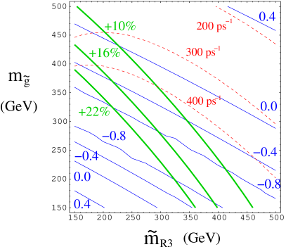
Figure 3: Contours of $S_{\phi K}$ (thin blue), percent increase in $BR(b\rightarrow s\gamma)$ (thick green), and $\Delta M_{B_{s}}$ (dashed red) for $\tilde{m}_{R2}=5$ TeV, optimal mixing angle and phase, and $\kappa=-1.1$ (left) and $\kappa=-2.0$ (right).

Generally speaking, lighter squark and gluino masses increase the effect of the new physics contributions, allowing $S_{\phi K}$ to depart from the standard model expectation. But at the same time this increases the contribution to $BR(b\rightarrow s\gamma)$ and runs up against the experimental constraint.

In Figure 4 we plot the same contours as a function of the gluino mass and the heavier squark mass $\tilde{m}_{R2}$, with $\tilde{m}_{R3}=300$ GeV. For $\kappa=-1.1$ there is a range of gluino masses where $S_{\phi K}$ can be below zero while still satisfying the $b\rightarrow s\gamma$ constraint. The minimum possible $S_{\phi K}$ allowed by this constraint decreases as the magnitude of $\kappa$ increases. For example, with $\kappa=-2.0$ the minimum value of $S_{\phi K}$ is roughly $-0.8$.

Finally in Figure 5 we plot the same contours as a function of the gluino mass and $\kappa$ with $\tilde{m}_{R2}=5$ TeV and $\tilde{m}_{R3}=300$ GeV. The $b\rightarrow s\gamma$ constraint is independent of $\kappa$, and we see how $S_{\phi K}$ decreases with the increasing magnitude of $\kappa$.

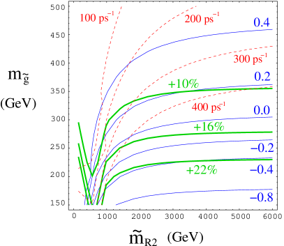
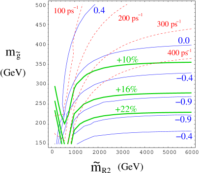
Figure 4: Contours of $S_{\phi K}$ (thin blue), percent increase in $BR(b\rightarrow s\gamma)$ (thick green), and $\Delta M_{B_{s}}$ (dashed red) for $\tilde{m}_{R3}=300$ GeV, optimal mixing angle and phase, and $\kappa=-1.1$ (left) and $\kappa=-2.0$ (right).

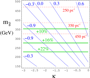
Figure 5: Contours of $S_{\phi K}$ (thin blue), percent increase in $BR(b\rightarrow s\gamma)$ (thick green), and $\Delta M_{B_{s}}$ (dashed red) for $\tilde{m}_{R2}=5$ TeV, $\tilde{m}_{R3}=300$ GeV, and optimal mixing angle and phase.

2.4.2 Dominant $LR+RR$ Mixing

Now we consider a second limiting case, where the diagonal left-right mixing leads to the dominant contribution to the $b$-quark decays. The contribution from $LR+RR$ mixing is enhanced in the dipole operators, so we may focus our attention on the coefficients $C^{\prime}_{g}$ and $C^{\prime}_{\gamma}$. To evade the constraint from $b\rightarrow s\gamma$, while simultaneously getting a large effect in $S_{\phi K}$, we want to minimize the ratio $C^{\prime}_{\gamma}/C^{\prime}_{g}$, which can be done by taking larger values of $x$, i.e. squark masses much heavier than the gluino.

In Figure 6 we reproduce Figure 3 but with a large value of $\mu\tan\beta\sim 35$ TeV. In this region the lightest squark mass eigenvalue, $\tilde{m}_{R3}$, needs to be above 1 TeV to avoid the bound from $b\rightarrow s\gamma$. For $\kappa=-1.1$ the smallest $S_{\phi K}$ can be is about $-0.4$ for a small gluino mass, while for $\kappa=-2.0$ any value is possible. In this case the $\kappa$-dependence is very simple because the main contribution to $S_{\phi K}$ comes from a single operator $\mathcal{O}^{\prime}_{g}$ whose contribution is directly proportional to $\kappa$. Thus an increased absolute value of $\kappa$ directly increases the effect in $S_{\phi K}$ without affecting the bound from $b\rightarrow s\gamma$.

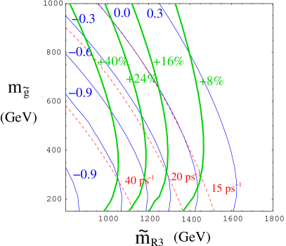
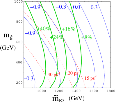
Figure 6: Contours of $S_{\phi K}$ (thin blue), percent increase in $BR(b\rightarrow s\gamma)$ (thick green), and $\Delta M_{B_{s}}$ (dashed red) for $\tilde{m}_{L2},\,\tilde{m}_{L3},\,\tilde{m}_{R2}\sim 2$ TeV, optimal mixing angles and phases, $\mu\tan\beta\sim 35$ TeV, and $\kappa=-1.1$ (left) and $\kappa=-2.0$ (right).

2.4.3 Combination of Contributions

In order to ascertain the relevance of each of these two regimes we scanned over the parameter space searching for the minimal values of $S_{\phi K}$ as a function of the product $\mu\tan\beta$. The result is shown in Figure 7 for sevaral values of $\kappa$. From the figure it is clear that for $\kappa=-1.1$ there is a slightly larger effect on $S_{\phi K}$ for larger values of $\mu\tan\beta$, though the entire region allows for a substantial deviation from the standard model. Notice that once $\kappa$ reaches $-2.0$ any value of $S_{\phi K}$ is possible.

To get a sense for the relative size of the $RR$ and $LR+RR$ contributions to $S_{\phi K}$, we can compare the magnitude of the two terms comprising $C^{\prime}_{g}$, Equation (19). Not surprisingly, for $\mu\tan\beta$ greater than about 25 TeV the $LR+RR$ contribution dominates by an order of magnitude. However, even for $\mu\tan\beta<1$ TeV there can be points where the $LR+RR$ contribution to the chromo-dipole operator is just as important as the $RR$ contribution. This underscores the importance of treating this calculation in the mass eigenbasis.

Figure 7: Minimum values of $S_{\phi K}$ as a function of $\mu\tan\beta$ for various values of $\kappa$ resulting from a scan of 58 million points that satisfied the $b\rightarrow s\gamma$ constraint. Note that $\kappa=-2.0$ can give $S_{\phi K}=-1.0$ for all values of $\mu\tan\beta$.

3 $B_{s}$ Mixing

Mixing between $\tilde{b}_{R}$ and $\tilde{s}_{R}$ also leads to a significant contribution to $B_{s}$-$\bar{B}_{s}$ mixing. In our scenario the effective Hamiltonian that receives such contributions consists of three operators that have nonzero coefficients:

$$\mathcal{H}_{\mathrm{eff}}^{SUSY}=C^{V}_{RR}(\bar{s}\gamma^{\mu}P_{R}b)(\bar{s}\gamma_{\mu}P_{R}b)+C^{S}_{LL}(\bar{s}P_{L}b)(\bar{s}P_{L}b)+C^{S\times}_{LL}(\bar{s}_{i}P_{L}b_{j})(\bar{s}_{j}P_{L}b_{i}).$$ (34)

The Wilson coefficients at the high scale are obtained by matching the effective Hamiltonian to the $\Delta B=2$ squark-gluino box diagrams like those shown in Figure 8. The result is given by:

$$C^{V}_{RR} = \frac{\alpha_{s}^{2}}{m_{\tilde{g}}^{2}}\sum_{AB}\Gamma^{R*}_{sA}\Gamma^{R}_{bA}\Gamma^{R*}_{sB}\Gamma^{R}_{bB}\times\left[-\frac{11}{9}B_{1}(x_{A},x_{B})-\frac{1}{9}B_{2}(x_{A},x_{B})\right]$$ (35)

$$C^{S}_{LL} = \frac{\alpha_{s}^{2}}{m_{\tilde{g}}^{2}}\sum_{AB}\Gamma^{R*}_{sA}\Gamma^{L}_{bA}\Gamma^{R*}_{sB}\Gamma^{L}_{bB}\times\left[-\frac{17}{18}B_{2}(x_{A},x_{B})\right]$$ (36)

$$C^{S\times}_{LL} = \frac{\alpha_{s}^{2}}{m_{\tilde{g}}^{2}}\sum_{AB}\Gamma^{R*}_{sA}\Gamma^{L}_{bA}\Gamma^{R*}_{sB}\Gamma^{L}_{bB}\times\left[\frac{1}{6}B_{2}(x_{A},x_{B})\right],$$ (37)

where the loop-functions are defined in Appendix A, the $\Gamma$’s are defined in Equation (12), and again $x_{A}=\tilde{m}_{A}^{2}/m^{2}_{\tilde{g}}$.

Figure 8: Diagrams contributing to $B_{s}$-mixing through large $\tilde{b}_{R}$-$\tilde{s}_{R}$ mixing. The diagram on the right induces effective $\tilde{b}_{L}$-$\tilde{s}_{R}$ mixing which contributes to $C_{LL}^{S}$ and $C_{LL}^{S\times}$.

The leading Standard Model contribution to $B_{s}$ mixing is induced by a top quark box diagram which yields the following effective Hamiltonian [14]

$$\mathcal{H}_{\mathrm{eff}}^{SM}=C_{LL}^{SM}(\bar{s}\gamma^{\mu}P_{L}b)(\bar{s}\gamma_{\mu}P_{L}b),$$ (38)

with the Wilson coefficient matched at $M_{W}$

$$C_{LL}^{SM}=\frac{G_{F}^{2}}{16\pi^{2}}M_{W}^{2}\left(V_{ts}^{*}V_{tb}\right)^{2}S(m_{t}^{2}/M_{W}^{2}),$$ (39)

where

$$S(x)=\frac{4x-11x^{2}+x^{3}}{4(1-x)^{2}}-\frac{2x^{3}\ln x}{2(1-x)^{3}}.$$ (40)

Before taking the hadronic matrix element of the effective Hamiltonian we must first take QCD corrections into account by using the renormalization group equations (RGE) to evolve the Wilson coefficients down to the low scale. The general NLO running of the Wilson coefficients for a $\Delta B=2$ effective Hamiltonian is given in [21] and [22] and involves mixing among different coefficients. In our case only the two scalar left-left operators mix, while the vector right-right and the vector-left-left coefficients simply scale multiplicatively. For simplicity we have evolved both operators from $M_{W}$ down to the mass of the $b$-quark.

The hadronic matrix element of the effective Hamiltonian between $B_{s}$ and $\bar{B}_{s}$ states was calculated on the lattice [23]

$$\langle\bar{B}_{s}\left|(\bar{s}\gamma^{\mu}P_{R}b)(\bar{s}\gamma_{\mu}P_{R}b)\right|B_{s}\rangle = \frac{1}{3}m_{B_{s}}f^{2}_{B_{s}}B_{1}(\mu)$$ (41)

$$\langle\bar{B}_{s}\left|(\bar{s}P_{L}b)(\bar{s}P_{L}b)\right|B_{s}\rangle = -\frac{5}{24}\left(\frac{M_{B_{s}}}{m_{b}+m_{s}}\right)^{2}m_{B_{s}}f^{2}_{B_{s}}B_{2}(\mu)$$ (42)

$$\langle\bar{B}_{s}\left|(\bar{s}_{i}P_{L}b_{j})(\bar{s}_{j}P_{L}b_{i})\right|B_{s}\rangle = \frac{1}{24}\left(\frac{M_{B_{s}}}{m_{b}+m_{s}}\right)^{2}m_{B_{s}}f^{2}_{B_{s}}B_{3}(\mu),$$ (43)

with $f_{B_{s}}$ as given in Table 1, $B_{1}(m_{b})=0.87(4)^{+5}_{-4}$, $B_{2}(m_{b})=0.82(3)(4)$, and $B_{3}(m_{b})=1.02(6)(9)$, where the first error is statistical and the second is systematic, excluding uncertainty due to quenching. The quark masses in the above expression should be evaluated at the scale $\mu$. The hadronic matrix element for the left-left current operator of the Standard Model is identical to that of the right-right operator shown in Equation (41). Finally, we can write the expression for the mass difference between $B_{s}$ and $\bar{B}_{s}$ as

$$\Delta M_{B_{s}}=2\left|\langle\bar{B}_{s}\left|\mathcal{H}_{\mathrm{eff}}^{\Delta B=2}\right|B_{s}\rangle\right|.$$ (44)

The Standard Model and supersymmetric contributions interfere, $\mathcal{H}_{\mathrm{eff}}^{\Delta B=2}=\mathcal{H}_{\mathrm{eff}}^{SM}+\mathcal{H}_{\mathrm{eff}}^{SUSY}$.

The input parameters used in the calculation are given in Table 1. Our results should be compared to the standard model prediction which can be obtained roughly by taking $\mathcal{H}_{\mathrm{eff}}^{\Delta B=2}=\mathcal{H}_{\mathrm{eff}}^{SM}$ in Equation (44), which yields $\Delta M_{B_{s}}^{SM}\sim 13.8\mbox{ ps}^{-1}$. A more rigorous treatment given in [24] yields

$$\Delta M_{B_{s}}^{SM}=17.3^{+1.5}_{-0.7}\mbox{ ps}^{-1}.$$ (45)

However, given the substantial uncertainty in the lattice evaluation of, e.g., $f_{B_{s}}$, it is probably appropriate to inflate this error, likely to the 25$\%$ level [25]. The current experimental limit, combining results from the LEP experiments and SLD, is [26]

$$\Delta M_{B_{s}}>14.4\mbox{ ps}^{-1}\mbox{ (95 \% confidence level)}.$$ (46)

Current and upcoming experiments are expected to be sensitive to mass differences much greater than the Standard Model prediction shown in Equation (45). At Run II of the Tevatron [27] CDF is expected to probe up to $\Delta M_{B_{s}}$ of 41 ps^-1 while BTeV is expected to achieve sensitivity to values up to $\Delta M_{B_{s}}\sim 55$ ps^-1. Any evidence that $\Delta M_{B_{s}}>25$ ps^-1 from these experiments would be a clear signal of new physics.

Parameter	Value	Parameter	Value	Parameter	Value
$m_{b}$	4.2 GeV	$m_{B_{s}}$	5.379 GeV	$V_{ts}^{*}V_{tb}$	$-$0.04
$m_{t}$	174 GeV	$f_{B_{s}}$	204 MeV	$\alpha_{s}(M_{Z})$	0.1185
$M_{W}$	80.4 GeV	$M_{Z}$	91.2 GeV	$\tau_{B_{s}}$	1.461 ps

Table 1: Input parameters used in the calculation of $S_{\phi K}$ and $\Delta M_{B_{s}}$.

To illustrate our results we add contours of constant $\Delta M_{B_{s}}$ (red dashed lines) to Figures 3-6. In the case of dominant right-right contributions, i.e. small $\mu\tan\beta$, the trend is similar to that of the previous section; lighter gluino and squarks give a larger SUSY contribution and thus increase $\Delta M_{B_{s}}$. Note that the supersymmetric contribution to the mass difference dominates over the Standard Model in significant regions of the supersymmetric parameter space, easily allowing $\Delta M_{B_{s}}>100\mbox{ ps}^{-1}$ where right-right mixing dominates. Such values for $\Delta M_{B_{s}}$ are certainly beyond the reach of the experiments mentioned above.

In the case of dominant $LR+RR$ mixing the modification of $B_{s}$ mixing is not as striking. In the example given in Figure 6 values of $\Delta M_{B_{s}}$ are much closer to the standard model prediction. Restricting ourselves to areas that respect the $b\to s\gamma$ bound gives a yet lower value, within the reach of upcoming experiments. We should point out that this is not generic since Figure 6 only represents a slice of parameter space. Other choices of parameters can give higher values of $\Delta M_{B_{s}}$ (above 30 $\mbox{ps}^{-1}$) for high values of $\mu\tan\beta$. The correlation of these results to those in $B_{d}^{0}\to\phi K_{S}$ will be discussed in the next section.

Finally, we should comment about possible CP violation in the $B_{s}$-$\bar{B}_{s}$ system. In the standard CKM scenario the $B_{s}\rightarrow\bar{B}_{s}$ amplitude does not have a CP violating phase (in the Wolfenstein parameterization), so no indirect CP violation is expected. In our scenario, however, $B_{s}$ mixing can involve the phases from the down-squark mass matrix. In the cases where the SUSY contribution to $B_{s}$ mixing dominates the SM, measurements of CP violation in $B_{s}\to J/\psi\phi$ will be sensitive to these phases.

4 Correlation

In this section we will discuss the correlation between $S_{\phi K}$ and $\Delta M_{B_{s}}$ in the context of large $\tilde{b}$-$\tilde{s}$ mixing. Because the effect on $B_{s}$ mixing is very different for the two limiting regions of parameter space, we will discuss them separately. For related studies see [12, 28].

4.1 Dominant $RR$ Mixing

In this region of parameter space the operators $\mathcal{O}^{\prime}_{3-6}$ make large contributions to $S_{\phi K}$, while there is essentially only one contribution to $B_{s}$ mixing, namely that from the operator shown in Equation (35). Unfortunately there is no simple, precise, relationship between the combination of the $\Delta B=1$ operators and the operator responsible for $B_{s}$ mixing. In general, they depend quite differently on loop functions.

In spite of this, one can make the following strong statement. In cases where there is a large shift in $S_{\phi K}$ away from the Standard Model expectation due to the operators $\mathcal{O}^{\prime}_{3-6}$, and the $RR$ contribution to $\mathcal{O}^{\prime}_{g}$ (the dominant right-right mixing scenario), there is a large contribution to $B_{s}$ mixing. To see this, we first note that the squarks and gluino must not be too heavy, and the $\tilde{b}$-$\tilde{s}$ mixing must be large in order to have a large contribution to $S_{\phi K}$. This suggests a minimum contribution to the $B_{s}$ mixing. However, there is the worry that it might be possible to fine-tune parameters to somehow drastically suppress the contribution to $B_{s}$ mixing; for example, by choosing squark and gluino mass ratios to minimize the value of the functions $B_{1}$ and $B_{2}$ in Equation (35). We find that this is not possible, however. In order to have a very large contribution to $S_{\phi K}$, one is pushed into a region of parameter space where the gluino, and at least one of the down-type squarks is light. Furthermore, the splitting between this light squark, which represents a mixture of $\tilde{b}$ and $\tilde{s}$ squarks, and the masses of the heavier squarks must be large to avoid a super-GIM cancellation. Once this qualitative picture for the spectrum is identified, it is easy to check that there cannot be a cancellation of the contribution to $B_{s}$ mixing in this case.

Now we present our results quantitatively. Since our goal here will be to show that large deviations in $S_{\phi K}$ will correspond to large contributions to $B_{s}$ mixing, we plot the minimum achievable value of $\Delta M_{B_{s}}$ for a given value of $S_{\phi K}$. The minimum is found by scanning a parameter space that consists of the parameters $\{m_{\tilde{g}},\tilde{m}_{L2},\tilde{m}_{R2},\tilde{m}_{R3},\cos\theta_{56},\phi_{6}\}$. As discussed in Equation (12), $\cos\theta_{56}$ represents the mixing angle between the right-handed $\tilde{b}$ and $\tilde{s}$ squarks, and $\phi_{6}$ represents the phase corresponding to this off-diagonal term. As a parameter space, we take:

$$m_{\tilde{g}} \in (200,700)\mbox{ GeV}$$ (47)

$$\tilde{m}_{L2} \in (300,2500)\mbox{ GeV}$$

$$\tilde{m}_{R2} \in (300,2500)\mbox{ GeV}$$

$$\tilde{m}_{R3} \in (250,1000)\mbox{ GeV}$$

$$\theta_{56} \in (0,\pi/2)$$

$$\phi_{6} \in (0,2\pi).$$

The lower limits on the masses are motivated by direct searches, while the upper limits are motivated by naturalness considerations. A scan would generate a scatter plot of $S_{\phi K}$ vs. $\Delta M_{B_{s}}$. For a given resultant value of $S_{\phi K}$, we find the combination of parameters that yields the smallest contribution to $B_{s}$ mixing. This is essentially equivalent to taking the boundary of the region generated by the scatter plot.

As discussed in Section 2, there is considerable dependence on the variable $\kappa$, which has a relatively large uncertainty. So we repeat the above exercise for several values of $\kappa$, displaying the results in Figure 9. Adding the constraint from $b\rightarrow s\gamma$ modifies these results as shown in Figure 10. The contours in Figure 10 notably do not extend as low in $S_{\phi K}$ because the $b\rightarrow s\gamma$ constraint removes the region of parameter space that allowed us to obtain those values in Figure 9.

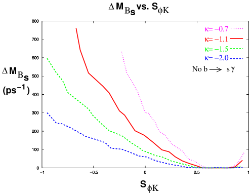
Figure 9: The minimum value of $\Delta M_{B_{s}}$ for a given value of $S_{\phi K}$. It is found by scanning over the parameter space given in Equation (47). The corresponding curve is shown for several values of $\kappa$, the coefficient of the dipole operator, as defined in Equation (23).

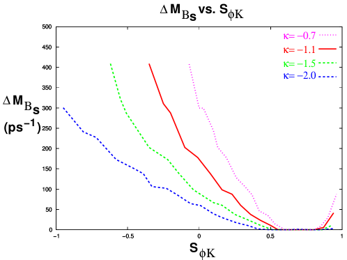
Figure 10: The same as Figure 9, but with the $b\rightarrow s\gamma$ constraint applied as discussed in the text. The minimum value of $\Delta M_{B_{s}}$ for a given value of $S_{\phi K}$. It is found by scanning over the parameter space given in Equation (47). The corresponding curve is shown for several values of $\kappa$, the coefficient of the dipole operator, as defined in Equation (23).

The take-home message from the figures is a simple one. If the hint of the deviation in $S_{\phi K}$ measured in the $B\rightarrow\phi K_{S}$ persists and it is attributable to a scenario with dominant $RR$ squark mixing, it will result in a large contribution to $B_{s}$ mixing, which will be a clear indication of new physics observable at the Tevatron.

4.2 Dominant $LR+RR$ Mixing

In the region of parameter space where $\mu\tan\beta$ is relatively large, the expectation for $\Delta M_{B_{s}}$ is very different. In this region the main contribution to $S_{\phi K}$ comes from the $LR+RR$ contribution to the dipole operator $\mathcal{O}^{\prime}_{g}$. This contribution can be sizeable even when the squarks and gluinos are heavy (squarks can be at the TeV level or higher). This is the significant difference between the two limiting cases. Heavy squarks and gluino mean that the contributions from the operators $\mathcal{O}^{\prime}_{3-6}$ are small. Similarly, the operators responsible for $B_{s}$ mixing, which come from box diagrams and resemble $\mathcal{O}^{\prime}_{3-6}$, can also be small. The bottom line is that a large contribution to $S_{\phi K}$ is possible without a large addition to $\Delta M_{B_{s}}$. This is borne out numerically, as shown in Figure 6, where the points allowed by the $b\rightarrow s\gamma$ constraint all give $\Delta M_{B_{s}}$ very close to the Standard Model expectation.

We have seen that the $LR+RR$ contribution to $S_{\phi K}$ can be important even for fairly small values of $\mu\tan\beta$, so it is natural to wonder what conclusions can be drawn about $\Delta M_{B_{s}}$ in the regions where both contributions are important. To answer this question we again performed a scan of the parameter space, this time collecting points with maximal and minimal $\Delta M_{B_{s}}$ as a function of $\mu\tan\beta$ with the additional requirement that $S_{\phi K}<-0.2$ for the nominal value $\kappa=-1.1$. The results are shown in Figure 11. In accord with what was stated above, points with the largest $\mu\tan\beta$ give smaller contributions to $B_{s}$ mixing. In fact, for $\mu\tan\beta>40$ TeV any effects on $\Delta M_{B_{s}}$ will be indistinguishable from the Standard Model expectation. This apparent upper bound may be interpreted as follows. For large $\mu\tan\beta$ the severe $b\to s\gamma$ bound is pushing us to regions where $RR$ mixing is small or masses are high, both of which disfavor large contributions to $B_{s}$ mixing. At the other end of the spectrum, for $\mu\tan\beta<2.4$ TeV all points in the scan gave values of $\Delta M_{B_{s}}>30$ ps^-1, a clear signal of new physics above even the largest Standard Model predictions. This trend continuously connects us back to the result of the previous subsection.

Figure 11: Maximum and minimum values of $\Delta M_{B_{s}}$ as a function of $\mu\tan\beta$ resulting from a scan of 150000 points in the parameter space with $S_{\phi K}<-0.2$ and $\kappa=-1.1$. The plot on the left shows an enlargement of the region of small $\mu\tan\beta$.

Mixing between the first two generations of squarks has fallen outside the main scope of this paper. We should mention, however, that larger values of the lightest squark masses, around 500 GeV, may well be preferred by constraints from $K$-$\bar{K}$ mixing. To see this, note that if we believe that the Cabibbo angle originates through the down Yukawa matrices, then the down Yukawa matrix has the structure:

$$\mathbf{\lambda}_{d}=\left(\begin{array}[]{cc}h_{d}&h_{s}\lambda_{C}\\ h&h_{s}\\ \end{array}\right),$$ (48)

where $h$ is some unknown Yukawa coupling and $\lambda_{C}$ is the sine of the Cabibbo angle. Diagonalizing this matrix requires a rotation on $d_{L}$ and $s_{L}$ of ${\mathcal{O}}(\lambda_{C})$ which induces an off-diagonal element of order $h_{d}\lambda_{C}$. Using the phenomenological relationship, $m_{d}/m_{s}\approx\lambda_{C}^{2}$, we find that a rotation between $d_{R}$ and $s_{R}$ of ${\mathcal{O}}(\lambda_{C}^{3})$ is needed to complete the diagonalization. Then, due to the lack of degeneracy between the squarks, the induced $\tilde{d}$-$\tilde{s}$ mixing can lead to a large contribution to the $K$-$\bar{K}$ mixing. This suggests that heavier squark masses, perhaps above 500 GeV are preferred, barring some accidental cancellation with the (unknown) $(1,2)$ element, $h$, in the above matrix.

By the above reasoning, if one wishes to achieve an $S_{\phi K}$ that differs significantly from the value of $\sin 2\beta$ as measured in the in the $B_{d}^{0}\rightarrow J/\psi K_{S}$ channel, there may a theoretical prejudice to prefer scenarios where large squark masses are more easily accommodated, such as the $LR+RR$ dominant case or the $RR$ dominant case in conjunction with a large value of $\kappa$.

5 Conclusion

There exist a class of models, motivated by Grand Unified theories and the large observed mixing in atmospheric neutrinos, where it is natural to have a large mixing between the right-handed $\tilde{b}$ squark and $\tilde{s}$ squark. We have found that there exists a range of parameters where such mixing induces a significant deviation in $S_{\phi K}$ from the Standard Model expectation of $\sin 2\beta$ as measured in the channel $B_{d}^{0}\rightarrow J/\psi K_{S}$.

In particular, the central value for $S_{\phi K}$ from BaBar and BELLE can be accommodated without conflicting with the measured value of $b\rightarrow s\gamma$, using the naive estimate for $\kappa$, the hadronic matrix element for the chromo-dipole operator. For larger values of $\kappa$ any value of $S_{\phi K}$ is allowed within the constraint.

There are two possible origins of a substantial modification to $S_{\phi K}$. The first solely involves a large right-right mixing, with no contribution from the mixing proportional to $m_{b}\mu\tan\beta$. In this case a small gluino mass is required, near the experimental bound. Correspondingly, there is a large contribution to $B_{s}$ mixing, a consequence which will be testable at the Tevatron Run II. In the second case, we consider the mixing from the combination of the large right-right mixing and a large $m_{b}\mu\tan\beta$. In this case, squarks and gluinos need not be light, so $B_{s}$ mixing need not be large. In particular, for very large values of $\mu\tan\beta$ the prediction for $B_{s}$ mixing is indistinguishable from the Standard Model prediction, when current errors on lattice matrix elements are taken into account. However, a substantial improvement in the Standard Model prediction for $B_{s}$ mixing still may allow an effect to be seen at the Tevatron in this case.

Note Added

While completing this paper we received References [29, 30]. There is some overlap with these papers, which also consider supersymmetric contributions to $B_{d}^{0}\to\phi K_{S}$.

Regarding [29], in places that we overlap, we agree qualitatively with their results, though there may be some quantitative differences. These are likely due to the fact that they work in the mass insertion approximation. Indeed, allowing large mixings and hierarchies that cannot be described by mass insertions gives us larger contributions in the ‘pure’ $RR$ mixing case. Other possible differences may arise from a different treatment of the hadronic matrix elements and the fact that constraints from $b\to s\gamma$ were not imposed in the same way.

We differ from both papers in our emphasis on the mixing induced by a combination of $m_{b}\mu\tan\beta$ along with a large flavor-changing $RR$ element in the squark mass matrix. Though double mass insertions are briefly discussed in [29], both [29] and [30] focus on the contributions of single mass insertions, including flavor off-diagonal $LR$ mixing.

We would like to emphasize that the double mass insertion ($LR+RR$ mixing) does not necessarily describe the same physics as a single $LR$ flavor mixing insertion, a point also mentioned in [29]. Treating a $LR+RR$ mixing as a pure $\delta_{23}^{RL}$ may miss important contributions due to the $RR$ mixing only. For example, we find maximal values of $\Delta M_{B_{s}}$ for intermediate values of $\mu\tan\beta$ which are much higher than those plotted in [29] with pure $LR$ mixing. This might be due to a $RR$ mixing contribution which is sub-dominant in $S_{\phi K}$ but which nevertheless gives a large contribution to $\Delta M_{B_{s}}$. This example illustrates how our framework differs from analyses which consider only one mass insertion at a time.

Appendix A Loop Functions

We include the loop functions for completeness. We use the same definitions as in [11]. Here $x_{A}\equiv m_{\tilde{d}_{A}}^{2}/m_{\tilde{g}}^{2}$.

$$B_{1}(x_{A},x_{B}) = \int_{0}^{\infty}\frac{-\frac{1}{4}z^{2}\,dz}{(z+1)^{2}(z+x_{A})(z+x_{B})}$$ (49)

$$= -\frac{x_{A}^{2}\log x_{A}}{4(x_{A}-x_{B})(x_{A}-1)^{2}}-\frac{x_{B}^{2}\log x_{B}}{4(x_{B}-x_{A})(x_{B}-1)^{2}}$$

$$-\frac{1}{4(x_{A}-1)(x_{B}-1)},$$

$$B_{2}(x_{A},x_{B}) = \int_{0}^{\infty}\frac{z\,dz}{(z+1)^{2}(z+x_{A})(z+x_{B})}$$ (50)

$$= -\frac{x_{A}\log x_{A}}{(x_{A}-x_{B})(x_{A}-1)^{2}}-\frac{x_{B}\log x_{B}}{(x_{B}-x_{A})(x_{B}-1)^{2}}$$

$$-\frac{1}{(x_{A}-1)(x_{B}-1)},$$

$$C_{1}(x) = \frac{2x^{3}-9x^{2}+18x-11-6\log x}{36(1-x)^{4}},$$ (51)

$$C_{2}(x) = \frac{-16x^{3}+45x^{2}-36x+7+6x^{2}(2x-3)\log x}{36(1-x)^{4}},$$ (52)

$$D_{1}(x) = \frac{-x^{3}+6x^{2}-3x-2-6x\log x}{6(1-x)^{4}},$$ (53)

$$D_{2}(x) = \frac{-x^{2}+1+2x\log x}{(x-1)^{3}},$$ (54)

$$D_{3}(x) = \frac{2x^{3}+3x^{2}-6x+1-6x^{2}\log x}{6(1-x)^{4}},$$ (55)

$$D_{4}(x) = \frac{-3x^{2}+4x-1+2x^{2}\log x}{(x-1)^{3}}.$$ (56)

Appendix B Chromo-dipole Matrix Element for $B_{d}^{0}\rightarrow\phi K_{S}$

In this appendix we show explicitly the computation of the matrix element of $\mathcal{O}^{(\prime)}_{g}$ in the naive factorization approximation. The computation of a similar quantity for $\bar{B}^{0}\rightarrow\pi^{+}\pi^{-}$ decay can be found in [31].

We start with

$$\mathcal{O}_{g}=\frac{g_{s}}{8\pi^{2}}m_{b}(\bar{s}_{i}\sigma^{\mu\nu}T^{a}_{ij}P_{R}b_{j})G^{a}_{\mu\nu}$$ (57)

and then connect a quark current through a virtual gluon to form a four-quark operator. This step depends on the convention used for the covariant derivative. Our convention is that $D_{\mu}=\partial_{\mu}+igT^{a}A^{a}_{\mu}$, and we have checked that this is consistent with the Wilson coefficients for both the standard model and SUSY contributions. This yields the operator

$$\mathcal{O}_{g4}=i\frac{\alpha_{s}}{\pi}\frac{k_{\nu}}{k^{2}}m_{b}(\bar{s}_{i}\sigma^{\mu\nu}T^{a}_{ij}P_{R}b_{j})(\bar{q}_{k}\gamma_{\mu}T^{a}_{k\ell}q_{\ell})$$ (58)

where $k=p_{b}-p_{s}$ is the gluon momentum. In the naive factorization approximation the color-octet current, $(\bar{q}_{k}\gamma_{\mu}T^{a}_{k\ell}q_{\ell})$, cannot produce a physical $\phi$, so the $\phi$ must be produced by the $\bar{s}$ and $q$ operators. To factor the matrix element we first use the equations of motion to simplify the tensor current. This yields:

$$\mathcal{O}_{g4}=-\frac{\alpha_{s}}{\pi k^{2}}m_{b}\left\{m_{b}(\bar{s}\gamma^{\mu}P_{L}T^{a}_{ij}b)+m_{s}(\bar{s}\gamma^{\mu}P_{R}T^{a}_{ij}b)-2p_{b}^{\mu}(\bar{s}_{i}P_{R}T^{a}_{ij}b_{j})\right\}\times$$

$$(\bar{q}_{k}\gamma_{\mu}T^{a}_{k\ell}q_{\ell})$$ (59)

where the last term was simplified using the conservation of the quark current, $k^{\mu}(\bar{q}_{k}\gamma_{\mu}T^{a}_{k\ell}q_{\ell})=0$ as in [31]. Then by a Fierz transformation and judicious use of Dirac matrix identities, this can be brought to the form [8, 32, 33]

$$\mathcal{O}_{g4} = -\frac{\alpha_{s}}{2\pi k^{2}}m_{b}\frac{N_{c}^{2}-1}{2N_{c}^{2}}\left(\delta_{i\ell}\delta_{kj}-\frac{2N_{c}}{N_{c}^{2}-1}T^{a}_{i\ell}T^{a}_{kj}\right)$$

$$\times\left[2m_{b}(\bar{s}_{i}\gamma^{\mu}P_{L}q_{\ell})(\bar{q}_{k}\gamma_{\mu}P_{L}b_{j})-4m_{b}(\bar{s}_{i}P_{R}q_{\ell})(\bar{q}_{k}P_{L}b_{j})\right.$$

$$\ \ \ \ +2m_{s}(\bar{s}_{i}\gamma^{\mu}P_{R}q_{\ell})(\bar{q}_{k}\gamma_{\mu}P_{R}b_{j})-4m_{s}(\bar{s}_{i}P_{L}q_{\ell})(\bar{q}_{k}P_{R}b_{j})$$

$$\ \ \ \ +2(p_{b})_{\mu}\left\{(\bar{s}_{i}\gamma^{\mu}P_{L}q_{\ell})(\bar{q}_{k}P_{R}b_{j})+(\bar{s}_{i}P_{R}q_{\ell})(\bar{q}_{k}\gamma^{\mu}P_{R}b_{j})\right.$$

$$\ \ \ \ \ \ \ \ \left.\left.+i(\bar{s}_{i}\sigma^{\mu\nu}P_{R}q_{\ell})(\bar{q}_{k}\gamma^{\nu}P_{R}b_{j})-i(\bar{s}_{i}\gamma_{\nu}P_{L}q_{\ell})(\bar{q}_{k}\sigma^{\mu\nu}P_{R}b_{j})\right\}\right]$$

Next we use the following parameterization for matrix elements.

$$\langle\phi(p_{\phi},\epsilon_{\phi})|\bar{s}\gamma^{\mu}s|0\rangle = f_{\phi}m^{2}_{\phi}\epsilon^{\mu}_{\phi}$$ (61)

$$\langle\phi(p_{\phi},\epsilon_{\phi})|\bar{s}s|0\rangle = 0$$ (62)

$$\langle\phi(p_{\phi},\epsilon_{\phi})|\bar{s}\sigma^{\mu\nu}s|0\rangle = -if_{\phi}m^{2}_{\phi}\frac{2m_{s}}{m_{\phi}^{2}}(\epsilon^{\mu}_{\phi}p^{\nu}_{\phi}-\epsilon^{\nu}_{\phi}p^{\mu}_{\phi}).$$ (63)

Also,

$$\langle\bar{K}^{0}(p_{K})|\bar{s}\gamma^{\mu}b|\bar{B}^{0}_{d}(p_{B})\rangle = (p_{B}+p_{K})^{\mu}F_{+}(t)$$ (64)

$$+ (p_{B}-p_{K})^{\mu}F_{-}(t)$$

$$\langle\bar{K}^{0}(p_{K})|\bar{s}b|\bar{B}^{0}_{d}(p_{B})\rangle = \delta_{bs}^{-1}\Delta_{BK}F_{+}(t)$$ (65)

$$+ \delta_{bs}^{-1}(p_{B}-p_{K})^{2}F_{-}(t)$$

$$\langle\bar{K}^{0}(p_{K})|\bar{s}\sigma^{\mu\nu}(1\pm\gamma_{5})b|\bar{B}^{0}_{d}(p_{B})\rangle = -2is(p_{B}^{\mu}p_{K}^{\nu}-p_{B}^{\nu}p_{K}^{\mu})$$ (66)

$$\pm s\varepsilon^{\mu\nu\lambda\sigma}(p_{B\lambda}p_{K\sigma}-p_{B\sigma}p_{K\lambda}).$$

Here $t=(p_{B}-p_{k})^{2}$, $\Delta_{BK}\equiv m_{B}^{2}-m_{K}^{2}$, and $\delta_{bs}\equiv m_{b}-m_{s}$. Notice we have corrected the sign in Equation (63) compared to the similar expression in [32]. Heavy quark effective theory gives the relation $s=(F_{+}-F_{-})/4m_{b}$ [34]. We also make the kinematic assumptions that the $b$-quark carries all of the $B$-meson momentum and that the $\phi$ momentum is equally divided between its two constituent $s$-quarks. Thus $p_{b}=p_{B}$ and $k^{2}=\frac{1}{2}(m_{B}^{2}-m_{\phi}^{2}/2+m_{K}^{2})$. Putting all the pieces together gives:

$$\kappa = -\frac{m_{b}^{2}}{2k^{2}}\left[1+\frac{m_{B}^{2}-m_{K}^{2}+m_{\phi}^{2}\frac{F_{-}}{F_{+}}}{4m_{b}(m_{b}-m_{s})}\right]$$ (67)

$$+ -\frac{m_{b}^{2}}{2k^{2}}\left[\frac{m_{K}^{2}-m_{B}^{2}-2m_{\phi}^{2}}{8m_{b}^{2}}\left(1-\frac{F_{-}}{F_{+}}\right)+\frac{m_{s}}{2m_{b}}\left(\frac{F_{-}}{F_{+}}\right)\right]$$

Because the matrix element is nonsingular we have $F_{-}(0)=0$. Then for small $t$, due to simple pole dominance we have $F_{-}(m_{\phi}^{2})\simeq F_{-}(0)=0$. [35] By ignoring the difference between $b$-quark and $B$-meson masses we arrive at the estimate cited earlier, $\kappa=-\frac{9}{8}+\mathcal{O}\left(\frac{m_{\phi}^{2}}{m_{B}^{2}}\right)\simeq-1.1$. The sign convention differs from [8], and the slight difference in magnitude can be traced to our replacement of $(p_{b}+p_{s})^{\mu}$ with $2p_{b}^{\mu}$ using the conservation of the added quark current. In [12] a similar quantity $\tilde{S}_{\phi K}=\frac{4}{9}\kappa$ is used. However, they quote a value $\tilde{S}_{\phi K}\simeq-0.76$ which appears to match $\tilde{S}_{\pi\pi}$ found in [31]. This would correspond to a value of $\kappa\simeq-1.71$.

References

• [1] Y. Fukuda et al. [Super-Kamiokande Collaboration], Phys. Rev. Lett.  81, 1562 (1998) [arXiv:hep-ex/9807003].
• [2] Q. R. Ahmad et al. [SNO Collaboration], Phys. Rev. Lett.  89, 011301 (2002) [arXiv:nucl-ex/0204008].
• [3] K. Eguchi et al. [KamLAND Collaboration], Phys. Rev. Lett.  90, 021802 (2003) [arXiv:hep-ex/0212021].
• [4] A. Alavi-Harati et al. [KTeV Collaboration], Phys. Rev. Lett.  83, 22 (1999) [arXiv:hep-ex/9905060];
V. Fanti et al. [NA48 Collaboration], Phys. Lett. B 465, 335 (1999) [arXiv:hep-ex/9909022].
• [5] B. Aubert et al. [BABAR Collaboration], Phys. Rev. Lett.  87, 091801 (2001) [arXiv:hep-ex/0107013];
K. Abe et al. [Belle Collaboration], Phys. Rev. Lett.  87, 091802 (2001) [arXiv:hep-ex/0107061].
• [6] D. Chang, A. Masiero and H. Murayama, arXiv:hep-ph/0205111.
• [7] Y. Grossman and M. P. Worah, Phys. Lett. B 395, 241 (1997) [arXiv:hep-ph/9612269].
• [8] R. Barbieri and A. Strumia, Nucl. Phys. B 508, 3 (1997) [arXiv:hep-ph/9704402].
• [9] B. Aubert et al. [BABAR Collaboration], arXiv:hep-ex/0207070;
T. Augushev, talk given at ICHEP 2002 (BELLE Collaboration), BELLE-CONF-0232.
• [10] G. Hiller, arXiv:hep-ph/0207356;
A. Datta, arXiv:hep-ph/0208016;
M. Raidal, arXiv:hep-ph/0208091;
J. P. Lee and K. Y. Lee, arXiv:hep-ph/0209290.
• [11] T. Moroi, Phys. Lett. B 493, 366 (2000) [arXiv:hep-ph/0007328].
• [12] E. Lunghi and D. Wyler, Phys. Lett. B 521, 320 (2001) [arXiv:hep-ph/0109149].
• [13] A. J. Buras, A. Romanino and L. Silvestrini, Nucl. Phys. B 520, 3 (1998) [arXiv:hep-ph/9712398];
G. Colangelo and G. Isidori, JHEP 9809, 009 (1998) [arXiv:hep-ph/9808487];
S. Baek, J. H. Jang, P. Ko and J. H. Park, Phys. Rev. D 62, 117701 (2000) [arXiv:hep-ph/9907572].
• [14] G. Buchalla, A. J. Buras and M. E. Lautenbacher, Rev. Mod. Phys.  68, 1125 (1996) [arXiv:hep-ph/9512380].
• [15] M. Ciuchini, E. Gabrielli and G. F. Giudice, Phys. Lett. B 388, 353 (1996) [Erratum-ibid. B 393, 489 (1997)] [arXiv:hep-ph/9604438].
• [16] F. Gabbiani, E. Gabrielli, A. Masiero and L. Silvestrini, Nucl. Phys. B 477, 321 (1996) [arXiv:hep-ph/9604387].
• [17] N. G. Deshpande and X. G. He, Phys. Rev. Lett.  74, 26 (1995) [Erratum-ibid.  74, 4099 (1995)] [arXiv:hep-ph/9408404].
• [18] P. Gambino and M. Misiak, Nucl. Phys. B 611, 338 (2001) [arXiv:hep-ph/0104034].
• [19] B. Aubert et al. [BaBar Collaboration], arXiv:hep-ex/0207076;
R. Barate et al. [ALEPH Collaboration], Phys. Lett. B 429, 169 (1998);
K. Abe et al. [Belle Collaboration], Phys. Lett. B 511, 151 (2001) [arXiv:hep-ex/0103042];
S. Chen et al. [CLEO Collaboration], Phys. Rev. Lett.  87, 251807 (2001) [arXiv:hep-ex/0108032].
• [20] J. S. Hagelin, S. Kelley and T. Tanaka, Nucl. Phys. B 415, 293 (1994).
• [21] A. J. Buras, M. Jamin and P. H. Weisz, Nucl. Phys. B 347, 491 (1990).
• [22] D. Becirevic et al., Nucl. Phys. B 634, 105 (2002) [arXiv:hep-ph/0112303].
• [23] D. Becirevic, V. Gimenez, G. Martinelli, M. Papinutto and J. Reyes, JHEP 0204, 025 (2002) [arXiv:hep-lat/0110091].
• [24] M. Ciuchini et al., JHEP 0107, 013 (2001) [arXiv:hep-ph/0012308].
• [25] A. S. Kronfeld and S. M. Ryan, Phys. Lett. B 543, 59 (2002) [arXiv:hep-ph/0206058].
• [26] LEP $B$-Oscillations Working Group, http://lepbosc.web.cern.ch/LEPBOSC/combined_results/amsterdam_2002/
• [27] K. Anikeev et al., arXiv:hep-ph/0201071.
• [28] Y. Grossman, M. Neubert and A. L. Kagan JHEP 9910, 029 (1999) [arXiv:hep-ph/9909297].
• [29] G. L. Kane, P. Ko, H. b. Wang, C. Kolda, J. H. Park and L. T. Wang, arXiv:hep-ph/0212092.
• [30] S. Khalil and E. Kou, Phys. Rev. D 67, 055009 (2003) [arXiv:hep-ph/0212023].
• [31] A. Arhrib, C. K. Chua and W. S. Hou, Eur. Phys. J. C 21, 567 (2001) [arXiv:hep-ph/0104122].
• [32] N. G. Deshpande, X. G. He and J. Trampetic, Phys. Lett. B 377, 161 (1996) [arXiv:hep-ph/9509346].
• [33] A. L. Kagan and A. A. Petrov, arXiv:hep-ph/9707354.
• [34] N. Isgur and M. B. Wise, Phys. Rev. D 42, 2388 (1990).
• [35] W. N. Cottingham, H. Mehrban and I. B. Whittingham, J. Phys. G 28, 2843 (2002) [arXiv:hep-ph/0102012].