Charged Higgs Production in the 1 TeV Domain as a
Probe of Supersymmetric Models

Abstract

We consider the production, at future lepton colliders, of charged Higgs pairs in supersymmetric models. Assuming a relatively light SUSY scenario, and working in the MSSM, we show that, for c.m. energies in the one TeV range, a one-loop logarithmic Sudakov expansion that includes an ”effective” next-to subleading order term is adequate to the expected level of experimental accuracy. We consider then the coefficient of the linear (subleading) SUSY Sudakov logarithm and the SUSY next to subleading term of the expansion and show that their dependence on the supersymmetric parameters of the model is drastically different. In particular the coefficient of the SUSY logarithm is only dependent on $\tan\beta$ while the next to subleading term depends on a larger set of SUSY parameters. This would allow to extract from the data separate informations and tests of the model.

I Introduction

In the last few years, a considerable effort has been devoted to the precise formulation of the theoretical predictions for electroweak effects in pair production at future lepton colliders. In particular, the considered center of mass (c.m.) energies have been those that represent the final goal of two proposed future machines, roughly one TeV for LC [1] and three TeV for CLIC [2]. The main motivation of the various investigations has been the fact that, within the electroweak sector of the SM, for c.m. energies of the few TeV size, it has been realized [3, 4, 5] that unexpectedly large virtual effects arise at the one loop level, that could make the validity of this (relatively) simple perturbative calculation highly debatable. These terms have the analogous dependence on energy as those originally determined in QED by Sudakov [6]; at one loop, they can either be of squared logarithmic (leading) (DL) or of linear logarithmic (subleading) (SL) kind, and their numerical effect in several observables breaks the ”safety” few percent limit (fixed by the aimed ( one percent) experimental accuracy) when one enters the few (2-3) TeV region, making the request of a higher order calculation to become imperative in that range.

Within the SM framework a resummation to all orders actually exists to next-to subleading order for final massless fermion pairs, and to subleading order for general massive final pairs [7]. In the (particularly relevant) case of massive final fermions a comparison (to subleading logarithmic accuracy) between one-loop and resummed expansions has been performed [8]. The results indicate that, for c.m. energies entering the few (2-3) TeV range, the discrepancies between the two approximations become intolerably (i.e. beyond a relative ten percent) large. On the contrary, for energies in the one TeV region, no appreciable difference shows up: to subleading order, the one-loop description appears there adequate. The question remains that of whether possible next-to subleading (for instance constant) terms might play a role.

For massive (third generation) final quark pairs, this problem was investigated in an “effective” way [9], trying to fit the exact one-loop calculation of a simple class of diagrams with a logarithmic expansion also containing an additional constant. The result was that, in the one TeV region, this fit was adequately describing the exact calculation, with the logarithmic coefficients exactly predicted by the Sudakov expansion and a constant term given by the fit. The size of this term was (relatively) “large”, about one half of the logarithmic contribution, with opposite sign (thus decreasing the overall effect). The apparent conclusion was that, in that energy range, a one-loop Sudakov expansion implemented by an extra constant term seems to be able to reproduce the exact calculation with an accuracy that is largely sufficient, at the expected experimental precision level of a relative one percent.

As a comment on the previous conclusion, it can be noticed that the possible experimental determination of the separate logarithmic and constant terms would not lead to any new information in the SM, since all the various coefficients will depend on the (fixed) known values of the SM parameters. In this sense, accurate measurements of massive (and massless) fermion pair production at LC in the one TeV region can only provide, in the SM framework, another experimental test of the validity of the model.

A natural question that arises at this stage is that of whether similar, or different, conclusions can be drawn for the simplest supersymmetric generalization of the SM that can still be treated perturbatively, i.e. the Minimal Supersymmetric Standard Model. This model and its Sudakov expansion has been actually already considered to subleading logarithmic accuracy in a number of papers, to the one-loop level for massless and massive fermion pairs [4, 5] and resumming to all orders for sfermion and Higgs production [10]. In the latter case, a comparison between the one-loop and the resummed expansion has also been performed under the assumption of a relatively light SUSY scenario, showing that, in strict analogy with the SM situation, the two calculations are essentially identical in the one TeV region, while deep differences show up in the (2,3) TeV energy range. No effort was made to try to estimate the size of a possible next to subleading term in the one-loop expansion in the one TeV region from a fit to the exact calculation, analogous to that performed in  [9] for the SM case.

The aim of this paper is precisely that of studying the feasibility and the possible advantages of performing an effective logarithmic one-loop expansion, implemented by a next-to subleading term, in the energy region around 1 TeV, for the MSSM. We anticipate that a preliminary necessary condition will be that of a light SUSY scenario, in which all the SUSY masses relevant for the considered process are supposed to be not heavier than a few hundred GeV. This means that the starting picture will be one where SUSY has already been discovered via direct production of (at least some) sparticles, so that a number of SUSY masses is already known and fixed. This is not obviously true for other quantities of the model, like for instance $\tan\beta$ or other parameters of the Higgs sector.

The purpose of our investigation will be that of showing that one fundamental differences will arise in the MSSM analysis with respect to the SM case. Our conclusion will be in fact that the coefficient of the SUSY Sudakov logarithm and the next to subleading term will exhibit a drastically different dependence on the parameter of the model, so that their possible experimental identification might lead to quite valuable information. In particular, we shall reconsider, in this new spirit, the possibility of a determination of $\tan\beta$, that is the only SUSY parameter on which the coefficient of the SUSY Sudakov (linear) logarithm depends, as already shown in previous papers [10, 11]. Also, we shall show that it is possible to investigate separately the dependence on the next to subleading term on the remaining SUSY parameters in the light scenario that we have assumed. In fact, we shall also show in some detail what is the range of SUSY parameters that may be considered ”light”, from the point of view of a Sudakov expansion like ours, in the one TeV region.

We should anticipate at this point the reason why we insist in calling the remaining, non logarithmic component of the asymptotic one-loop expansion ”next to subleading” term. In fact, we shall show that this remaining component cannot be rigorously considered as a constant in the investigated TeV region. To reproduce completely the exact calculation, one must add to the constant component an extra non logarithmic energy dependent quantity. As we shall show, though, this extra component is, at the expected level of accuracy, fairly ”small”. The consequence of its presence will be fully taken into account and will generate a realistic error in the determination of the SUSY parameter that we shall pursue.

As a first process to be examined in this spirit, we have chosen that of charged Higgs pair production. The main reason for this choice is that, from the point of view of the involved parameters, this is the simplest process to be considered in the MSSM. Our goal is that of moving in future papers to more complicated processes, following a logical chain that introduces gradually new parameters not already derived in this effective way. In order to provide a self-consistent and rigorous calculation device, we have completed a one loop code that contains all the relevant diagrams, in the approximation of treating all fermions as massless, with the exception of the third generation quarks. We have verified that the complete code does reproduce the correct(known) asymptotic logarithmic (DL and SL) behaviour. This complete code has been used to derive an effective next-to subleading Sudakov expansion, with which it has been imposed to it to agree to the few permille level. The code, that has been named SESAMO (Supersymmetric Effective Sudakov Asymptotic MOde), is already available for use [12].

Technically speaking, this paper will be organized as follows: Sec. II will contain the relevant asymptotic one loop expansions of the process. Sec. III will contain the comparison of the complete one loop calculation with the proposed effective fit as a function of the SUSY parameters. In Sec. IV, the determination of $\tan\beta$ and the study of the effect of the remaining parameters on the next-to subleading term will be examined and exhibited. A final discussion of our results in Sec. V will conclude the paper.

II Calculation of the process at one loop

A complete description of the scattering amplitude of the considered process at one loop requires the calculation of several classes of diagrams. To make our treatment as self-consistent as possible, we shall follow the notations used in a previous reference [10] and write:

$$A(e^{+}e^{-}\to H^{+}H^{-}) = A^{{\rm Born}}(e^{+}e^{-}\to H^{+}H^{-})+A^{c.t.}(e^{+}e^{-}\to H^{+}H^{-})$$ (3)

$$+A^{s.e.}(e^{+}e^{-}\to H^{+}H^{-})+A^{in}(e^{+}e^{-}\to H^{+}H^{-})$$

$$+A^{fin}(e^{+}e^{-}\to H^{+}H^{-})+A^{box}(e^{+}e^{-}\to H^{+}H^{-})+A^{QED}$$

It is convenient to normalize the general amplitude in the following way:

$$A={2e^{2}\over q^{2}}~{}\bar{v}(e^{+})(p\hskip-5.97527pt/)(a_{L}P_{L}+a_{R}P_{R})u(e^{-})$$ (4)

where $P_{L,R}=(1\mp\gamma^{5})/2$ and $p^{\mu}$ is the outgoing $H^{-}$ momentum, so that one writes the Born terms as:

$$a^{{\rm Born}}_{\lambda}=1-{(1-2s^{2}_{W})\over 4s^{2}_{W}c^{2}_{W}}\eta g_{e\lambda}$$ (5)

with $g_{eL}=2s^{2}_{W}-1,~{}~{}g_{eR}=2s^{2}_{W}$ and $\eta\equiv{q^{2}\over q^{2}-M^{2}_{Z}}$.

The remaining quantities represent the one-loop perturbative modifications of the tree level expression. More precisely, $A^{c.t.}$ is the contribution from the usual ”counter-terms” that cancel all the ultraviolet divergences of the process. In our chosen on-shell renormalization scheme, in which the inputs are $\alpha_{QED}(0)$, $M_{W}$ and $M_{Z}$, they are given by proper gauge boson self-energies, computed at the corresponding physical masses. Their explicit expressions are known (see e.g. [13]), and to save space we shall note write them here. $A^{s.e.}$ contains the various internal self-energy corrections; $A^{in,~{}fin}$ describe the initial and final vertex modifications and $A^{box}$ the box contributions. Their ”fine” structure is summarized in Appendix, where the various components of the separate terms are listed. The related complete set of Feynman diagrams is too large (more than 200 diagrams) to be drawn here; it can be found e.g. in a recent paper [14]. In our treatment, we have discarded those components that give contributions that vanish with the initial lepton mass, which reduces somehow our numerical calculations; (actually, we treated all fermions as massless, with the exception of the third family quarks). In our approach, ultraviolet divergences are produced both by self-energies and by vertices that include all external self-energies (we followed the definition proposed by Sirlin [15]). We checked that all the ultraviolet divergences in the scattering amplitude are mutually canceling. Finally, $A^{QED}$ represents our choice of the electromagnetic component. In this preliminary paper, we were mostly interested in the ”genuine” electroweak SUSY contributions at very high energies. For this reason, we treated all those virtual contributions with photons that would generate infrared divergences by introducing an ”effective” fictitious photon mass $M_{\gamma}=M_{Z}$. With this choice, our $A^{QED}$ will contain in fact the difference between these ”effective” terms and the conventional (massless photon) ones (with the usual request of adding the effects of real photon radiation when computing the cross section). This gives a contribution to the observables that, for our specific purposes, can be considered as ”known” since it does not involve any SUSY component, and will therefore not be included in our code at least at the moment. Its addition would not represent a problem, but would not add anything to the specific investigation of this paper, that is rather devoted to the ”unknown” component of the scattering amplitude.

In this spirit, we shall now write the overall logarithmic contributions to the scattering amplitude that arise at one loop in a proper configuration of ”asymptotic” energy. These are by definition the leading terms of an expansion made in a region where all the relevant (external and internal) masses are sufficiently smaller than the c.m. energy in a way that we shall try to make more quantitative in the following Section. In full generality, such logarithmic terms can be of two different origins. The first ones are linear logarithms of renormalization group (RG) origin, generated by gauge boson self-energies and representing the ”running” of the gauge coupling constants. Their expressions are known, and we shall write them explicitely but separately from the remaining terms. They do not contain any SUSY parameter, but must be carefully taken into account in our approach. The second ones are the genuine electroweak logarithms, nowadays generally called ”of Sudakov type”. They can be of quadratic and of linear kind; the quadratic ones come from vertices with single $W,~{}Z,~{}\gamma$ exchange and from boxes with two $W$ exchange and do not contain any SUSY parameter; the linear ones come from the remaining vertices and boxes and contain SUSY contributions only from vertices. A very special feature of the supersymmetric model that we have investigated and of the process that we have considered is that the only SUSY parameter that ”effectively” appears in the various linear logarithms is $\tan\beta$, of Yukawa origin, produced by the final vertices with ($b,~{}t$) exchange, that depends on the specific combination $[m^{2}_{t}\cot^{2}\beta+m^{2}_{b}\tan^{2}\beta]$ (SUSY mass parameters $M_{i}$, that could enter other vertex diagrams, would appear in the form $\log(q^{2}/M^{2}_{i})$, $\sqrt{q^{2}}$ is the c.m. energy, but with a suitable change of scale they can always be shifted into a constant term, as we shall show and discuss).

In Appendix we list the various logarithmic contributions coming from different diagrams. The convention that we have followed is that of keeping $M_{W}$ as the scale of the double $\log^{2}~{}q^{2}$ coming from two $W$ boxes and single $W$ vertices. For all the remaining logarithms we have chosen a common scale $M_{Z}$, with the exception of the Yukawa vertex where the most natural scale appears to us to be that of the top mass $m_{t}$. This choice is arbitrary, it is only dictated by our personal taste and feelings. The consequence of this choice will be that of fixing the numerical value of the ”next-to subleading” term. A pragmatic attitude would be that of verifying that, with this choice, both the logarithmic and the next-to subleading terms remain acceptably ”small” at the one loop level. This, as we shall show, will happen in fact and with this ”a posteriori” justification we shall retain our choice of scales.

From a glance to the Appendix one also sees that the linear $\log~{}q^{2}$ belong to two separate classes: the so-called ”universal” and the ”not universal” ones. The latter are produced by boxes and depend on the c.m. scattering angle $\vartheta$. We have already discussed in a previous paper [10] their different relevance at the one loop level, and we shall not insist here on these features. We can, though, recall the observed fact [10] that these $\vartheta$ dependent non universal terms are the only ones that contribute at logarithmic level the forward-backward asymmetries at one loop. Since they do not contain any SUSY parameter, as we said, there will be no relevant logarithmic contribution containing SUSY parameters to the forward-backward asymmetry of $H^{+}H^{-}$ production. The same conclusion can be derived for the longitudinal polarization asymmetry that is known to provide only information on the initial state as shown in the previous reference [10]. For this reason, we shall concentrate our numerical analysis on the total cross section of the process.

After this rather technical presentation, we are now ready to present the concrete numerical analysis. With this aim, we shall now summarize our previous discussion giving the asymptotic relative effect on the cross section of the process, by writing it in the form:

$$\Delta(q^{2})={\sigma^{{\rm Born+1loop}}-\sigma^{{\rm Born}}\over\sigma^{{\rm Born}}}$$ (6)

where in $\sigma^{{\rm Born+1loop}}$ we are retaining only the genuine one loop terms $\cal{O}(\alpha/\pi)$ and not the second order terms coming from the square of the one loop contributions since these mix with the genuine two loop contributions.

The logarithmic expansion of $\Delta$ has been derived analytically and is given by the expression

$$\Delta(q^{2}) = -~{}({\alpha\over 2\pi s^{2}_{W}})({1+2s^{4}_{W}\over 1+4s^{4}_{W}})\log^{2}{q^{2}\over M^{2}_{W}}$$ (11)

$$-~{}({\alpha\over 4\pi s^{2}_{W}c^{2}_{W}})({1+2s^{4}_{W}+8s^{6}_{W}\over 1+4s^{4}_{W}})\log^{2}{q^{2}\over M^{2}_{Z}}$$

$$-~{}({3\alpha\over 4\pi s^{2}_{W}M^{2}_{W}})(m^{2}_{t}\cot^{2}\beta+m^{2}_{b}\tan^{2}\beta)\log{q^{2}\over m^{2}_{t}}$$

$$+~{}({\alpha\over 3\pi s^{2}_{W}c^{2}_{W}})({11-16s^{2}_{W}+32s^{4}_{W}+72s^{6}_{W}\over 1+4s^{4}_{W}})\log{q^{2}\over M^{2}_{Z}}$$

$$+\Delta_{\rm rem}(q^{2})$$

where the fourth line contains all single logarithms with the exception of those of Yukawa origin (third line). The last term $\Delta_{\rm rem}(q^{2})$ is the difference between the full one loop result and its asymptotic Sudakov expansion including all the double and single logarithms, and will be called the next-to subleading term.

III Validity of the Sudakov expansion

The aim of this Section is that of investigating whether there exists a region of energy and of parameters where the rigorous calculation at one loop can be reproduced by the effective Sudakov expansion Eq.(11), and to determine the relevant features of the next-to subleading term $\Delta_{\rm rem}(q^{2})$. In order to avoid confusion, we anticipate that our analysis will be divided into two different sectors. In the first one, summarized in this Section, we shall study the dependence of $\Delta_{\rm rem}(q^{2})$ on the c.m. energy for given values of the parameters of the chosen MSSM model. In the second one, we shall study the dependence of $\Delta_{\rm rem}(q^{2})$ on the MSSM parameters for a fixed energy chosen at the representative 1 TeV value. To proceed with our analysis, we must now define the MSSM parameters that we shall use as input of the calculations. We retained the following five free parameters:

$$\tan\beta,~{}~{}~{}\mu,~{}~{}~{}M_{A},~{}~{}~{}M_{2},~{}~{}~{}M_{S}$$ (12)

i.e. the ratio of the two vevs, the Higgs bilinear coupling, the CP odd Higgs mass, the universal gaugino mass and the universal sfermion mass. For this preliminary analysis, we allowed ourselves the simplifications of using the GUT relation $M_{1}={5\over 3}\tan^{2}\vartheta_{W}M_{2}$ and of setting the trilinear couplings $A_{u}=A_{d}=0$. We computed the Higgs spectrum with the code FeynHiggsFast [16] and obtained the masses of charginos, neutralinos and sfermions by numerical diagonalization of their mixing matrices. We retained sfermion mixing only in the case of the third generation.

For the purposes of this paper, we have chosen to work in an energy region between 800 GeV and 1 TeV, considering 1 TeV as an ambitious conceivable final goal of the future LC. In our study, we shall assume that a number of precise measurements can be performed in that energy range, and we will show what could be the theoretical implications for the model in a particular region of its couplings and of its masses. Clearly, all the obtained informations and bounds on the various mass parameters could be easily rescaled if the analysis were performed in a lower (e.g. 600-800 GeV) energy interval.

The first problem that we address is that of determining the range of massive MSSM parameters for which the Sudakov expansion for $\Delta(q^{2})$ reproduces the rigorous calculation with a simple and understandable expression for the next-to subleading term $\Delta_{\rm rem}(q^{2})$. For the latter, the simplest possibility would be provided by a constant, and from our previous SM experience [10], we would be prepared to the appearance in this case of a relatively ”large” (i.e. compared to the logarithmic component) quantity. We cannot exclude, though, a priori the necessity of including an extra, energy dependent term, that should vanish at very large $\sqrt{q^{2}}$, but could be numerically relevant and complicated in the considered energy range. If this turned out to be the case, the practical validity of the Sudakov expansion would be unavoidably reduced, since every tentative effective fit to the data would be complicated and affected by large errors, and we shall return on this statement in the description of the derivation of $\tan\beta$, to be shown in the forthcoming Section.

Given the fact that we have to deal with four massive parameters, we have performed four different analyses, in each one of which three parameters were fixed at values that we considered ”light” with respect to the chosen energy range, and one parameter was allowed to vary. In all these analyses we fixed $\tan\beta$ at the value $\tan\beta=20$, that can be considered as an average value in the range that we have explored, roughly $2\lesssim\tan\beta\lesssim 40$ (we shall discuss later on the reasons of this choice of the upper value). Fixing different values of $\tan\beta$ does not change the results of the four analyses, that we chose in the following way:

1. variable $\mu$, fixed $M_{A}=200$ GeV, $M_{2}=100$ GeV, $M_{S}=350$ GeV;

2. variable $M_{A}$, fixed $\mu=300$ GeV, $M_{2}=100$ GeV, $M_{S}=350$ GeV;

3. variable $M_{2}$, fixed $\mu=300$ GeV, $M_{A}=200$ GeV, $M_{S}=350$ GeV;

4. variable $M_{S}$, fixed $\mu=300$ GeV, $M_{A}=200$ GeV, $M_{2}=100$ GeV;

The choices of the fixed values of the parameters in the four analyses are dictated by practical reasons and could be reasonably varied. The relatively small value of $M_{2}$ corresponds to the request of having relatively light charginos and neutralinos, although higher values $(\lesssim 300~{}\mbox{GeV})$ for $M_{2}$ would still be acceptable, as shown by Fig. (2). For $M_{A}$, the same considerations apply in order to avoid resonance formation. $M_{S}$ can vary in a larger range without apparent problems, and therefore it was fixed at a relatively higher value.

We are now ready to discuss the results of our analyses. This was performed by computing numerically the quantity $\Delta(q^{2})$ with the specific code (SESAMO) that we have built for our purposes and which is, we repeat, available for use. From the computed quantity we then subtracted all the logarithms of Eq.(11) and obtained the remaining, next-to subleading term $\Delta_{\rm rem}(q^{2})$.

An important preliminary remark must be made at this point. The final goal of our analysis is that of showing that a complete one-loop expression can be reproduced by a (relatively simple) Sudakov expansion. But a necessary condition to make this search useful is also that the one-loop expansion is reliable. To guarantee this condition, we shall have to verify that the complete expression of $\Delta(q^{2})$ (i.e. the full one-loop correction) remains acceptably small in the investigated energy region, with e.g. an upper bound that we could fix quantitatively at the relative ten percent value. Only after this check, our next analysis could be considered as meaningful.

We are now ready to show the results of the four considered cases, which are the following ones:

1) Case (a): variable $\mu$

We allowed $\mu$ to vary from an initial value of 300 GeV to final values of approximately 400 GeV (below 300 GeV, we encountered problems in the determination of the sfermion mass eigenstates whose discussion seems to us beyond the purposes of this preliminary analysis). The full one-loop effect, computed at the representative value $\sqrt{q^{2}}=1~{}\mbox{TeV}$, remains always very small (below two percent). The values of $\Delta_{\rm rem}(q^{2})$ in the interval $800~{}\mbox{GeV}\leq\sqrt{q^{2}}\leq 1~{}\mbox{TeV}$ are shown in Fig. (3). One sees that the term is changing by an amount roughly equal to five percent of its central value when moving from the beginning to the end of the interval. Numerically, this corresponds to a two permille effect that can be considered as ”fairly small” under our expected experimental conditions of a one percent accuracy. When $\mu$ becomes larger than roughly $380~{}\mbox{GeV}$, the simplicity of $\Delta_{\rm rem}(q^{2})$ is lost and a complicated energy dependence appears which is due to a resonance effect: when we increase $\mu$, one of the two charginos and two neutralinos become progressively heavier with masses $\sim\mu$. When $\mu\sim 400$ GeV, we begin to see a kinematical threshold at $\sim 800$ GeV that produces a bump in $\Delta_{\rm rem}$ well visible in the figure. Of course, the bump shifts to the right as $\mu$ is further increases. One observes also from Fig. (3) that $\Delta_{\rm rem}(q^{2})$ is scarcely affected by variations in $\mu$ (about half percent when $\mu$ varies from $300$ to $400$ GeV) and, as a consequence, it does not appear to be a promising candidate for testing virtual MSSM effects generated by this specific parameter.

We repeated our analysis changing only the sign of $\mu$. The obtained curves are practically (in agreement with our previous statement) identical with those corresponding to positive $\mu$ values. For this reason, we shall restrict ourselves from now on to considering conventionally the $\mu>0$ scenario.

2) Case (b): variable $M_{A}$

We have varied $M_{A}$ starting from an initial value of $200~{}\mbox{GeV}$ up to approximately $400~{}\mbox{GeV}$. The full (negative) one-loop effect at $1~{}\mbox{TeV}$ remains systematically below a relative two percent. As $M_{A}$ increases, the basic change in the spectrum of SUSY particles is that both $H^{+}$ and $H^{0}$ become heavier with approximately $M_{A^{0}}\sim M_{H^{0}}\sim M_{H^{+}}$. This means that in the plots we have to take into account the kinematical constraint $\sqrt{q^{2}}\geq 2M_{H^{+}}$. In Fig. (4) we show the behaviour of $\Delta_{\rm rem}$ for $200~{}\mbox{GeV}<M_{A}<400~{}\mbox{GeV}$. Once again, we notice that in the considered energy interval $\Delta_{\rm rem}(q^{2})$ remains ”essentially” constant, with relative extreme variations of five percent (or less) from its central value. This simple pattern would be lost for larger $M_{A}$ values $>400~{}\mbox{GeV}$, due to the aforementioned Higgs production threshold. One notices in this case that the dependence of $\Delta_{\rm rem}(q^{2})$ on $M_{A}$ is sizable: to a variation of $M_{A}$ from $200$ to $300~{}\mbox{GeV}$ there corresponds a variation in $\Delta_{\rm rem}(q^{2})$ of almost two percent, that would be visible at the proposed LC.

3) Case (c): variable $M_{2}$

Here, we vary $M_{2}$ from $100~{}\mbox{GeV}$ to $400~{}\mbox{GeV}$. The full one-loop effect at $1~{}\mbox{TeV}$ is again very small (below two percent) and negative. In the considered range of variation of $M_{2}$, there are one chargino and one neutralino with masses increasing approximately as $M_{2}$ and reaching the $400$ GeV value at which some resonance structure can be observed in the plots of $\Delta_{\rm rem}$ shown in Fig. (5). It can be noticed that, for $M_{2}$ larger than about $360$ GeV, the shape of this function is definitely not constant with energy and clear bumps can be seen, due to resonance effects associated to the heavy gauginos. As in the case of $\mu$, we observe that $\Delta_{\rm rem}(q^{2})$ has very small sensitivity to the variations of $M_{2}$ (about two permille variation for a $100~{}\mbox{GeV}$ shift in $M_{2}$).

4) Case (d): variable $M_{S}$

We have varied $M_{S}$ from $100~{}\mbox{GeV}$ to about $400~{}\mbox{GeV}$. The full one-loop effect is again very small and negative (below $\simeq 3-4$ percent). The values of $\Delta_{\rm rem}(q^{2})$ shown in Fig. (6) are again essentially (up to a relative $5$ percent) constant in the considered energy interval. One sees that $\Delta_{\rm rem}(q^{2})$ is sensitive to $M_{S}$: $100~{}\mbox{GeV}$ of variation in this parameter corresponds to $\simeq 1.5$ percent variation in $\Delta_{\rm rem}(q^{2})$.

To summarize, we have considered the range of validity of a logarithmic Sudakov expansion with an extra next-to subleading term which is ”essentially” constant in a certain domain of the massive MSSM parameters, for c.m. energies in the range $800~{}\mbox{GeV}-1~{}\mbox{TeV}$. In our approach, to be ”essentially” constant means to be well approximated by the central value, with a few permille error. We have verified that this requirement is met for values of all the parameters below, approximately, $350~{}\mbox{GeV}$. This gives a quantitative illustration of how ”light” the MSSM parameters should be in order that a typically asymptotic expansion like the Sudakov one that we investigate might hold at energies in the $1~{}\mbox{TeV}$ range. We can remark that, as matter of fact, the validity of the expansion corresponds to values of the masses meeting the naive request $M^{2}_{i}/q^{2}\lesssim 10^{-1}$. This remains true even if several resonances appear close to $\sqrt{q^{2}}/2$. In other words the energy dependence of this process appears to be reasonably flat in the considered domain. We also conclude that the values of the ”essentially” constant components are relatively ”large” and of opposite sign (positive) with respect to the (negative) logarithmic contribution (roughly, they are of comparable size, although always smaller than the logarithmic ones). As a result of this cancellation the overall one-loop effect is sensibly reduced, becoming systematically of few percent size. This situation reproduces exactly the one that we met in the analogous study of the SM case, even if the number of free parameters in the MSSM is so much larger.

A final question that we asked ourselves was that of whether the approximate constancy of $\Delta_{\rm rem}(q^{2})$ could be due to the relative smallness of the investigated energy domain. To answer this question, we have extended our analysis to very large $\sqrt{q^{2}}$ values up to $10~{}\mbox{TeV}$, for an illustrative fixed set of MSSM parameters

$$\tan\beta=30,\ \mu=300,\ M_{A}=200,\ M_{2}=100,\ M_{S}=350,$$ (13)

The results are shown in Fig. (7). One sees that for energies beyond $\simeq 2~{}\mbox{TeV}$ the values of $\Delta_{\rm rem}(q^{2})$ remain practically (i.e. to less than one permille) constant. Although we already know that at such energies the one-loop approximation is probably not valid, we consider this result as a check of the asymptotic validity of the expansion (and also of the numerical code that we have used).

In conclusion, we have seen that in the $1~{}\mbox{TeV}$ range a 1-loop Sudakov expansion with an ”essentially” constant term is valid for the defined ”light” SUSY scenario. The fact that $\Delta_{\rm rem}(q^{2})$ is not rigorously constant is expected to produce therefore reasonably ”small” effects, that we shall try to evidentiate in full detail in the forthcoming Section 4.

IV Study of the MSSM parameters

A Determination of $\tan\beta$

The first question that we address is the relevance of the Sudakov expansion for the problem of determining $\tan\beta$ under the assumption that the mass scales are in the “safe” range that we have just discussed. In other words, $\Delta_{\rm rem}$ is only approximately constant and we want to understand quantitatively how much this can affect an attempt to determine $\tan\beta$ from the logarithmic slope of the cross-section, in which it appears in the combination shown in Eq.(11).

With this aim, we begin by subtracting explicitly from $\Delta$ all the “known” logarithms, i.e. all the terms in the Sudakov expansion with the exception of the Yukawa contribution. Therefore, we define the quantity

$$\widetilde{\Delta}(q^{2}) = F(\tan\beta)\log\ q^{2}+\Delta_{\rm rem}(q^{2}),$$ (14)

$$F(\tan\beta) \equiv -\frac{3\alpha}{4\pi s_{\rm w}^{2}M_{W}^{2}}(m_{t}^{2}\cot^{2}\beta+m_{b}^{2}\tan^{2}\beta).$$ (15)

If, in a definite scenario, the shape of $\Delta_{\rm rem}(q^{2})$ turned out to be flat, then it would be conceivable to approximate it by a term that is constant with respect to $q^{2}$. In such a simple case, we could try to fit the measured values of the residual effect $\widetilde{\Delta}(q^{2})$ with a logarithmic expansion in $q^{2}$ of the form

$$A_{\rm fit}\log q^{2}+B_{\rm fit}.$$ (16)

The result of the fit, $A_{\rm fit}$, can be compared with $F$ at the value of $\tan\beta$ we are working. The difference $\delta F=A_{\rm fit}-F$ is an error in the estimate of $F$ that has two components: $\delta F=\delta_{\rm stat}F+\delta_{\rm sys}F$. The first term, $\delta_{\rm stat}F$ is simply due to the fact that we assume a certain finite experimental precision on each measurement. The second term, $\delta_{\rm sys}$ is the most important and is a systematic error due to the fact that $\Delta_{\rm rem}$ is not constant with respect to the energy. For instance, if $\Delta_{\rm rem}$ were exactly energy independent, we would find $\delta_{\rm sys}F=0$. The error $\delta F$ can be converted into an error on the estimate of the interesting parameter $\tan\beta$. If $\delta F/F$ is enough narrow to allow a linearized analysis, then we have simply

$$\frac{\delta F}{F}=\frac{\tan\beta\ F^{\prime}}{F}\ \frac{\delta\tan\beta}{\tan\beta}$$ (17)

or

$$\frac{\delta\tan\beta}{\tan\beta}=\frac{1}{2}\ \frac{\tan^{4}\beta+(m_{t}/m_{b})^{2}}{\tan^{4}\beta-(m_{t}/m_{b})^{2}}\ \frac{\delta F}{F}$$ (18)

The zero in the denominator corresponds to the value $\tan\beta=\sqrt{m_{t}/m_{b}}\simeq 6.2$ at which the function $F$ attains its maximum and the sensitivity to $\tan\beta$ is the smallest due to the flatness of $F$. Notice also that for $\tan\beta$ beyond $15-20$, we have

$$\frac{\delta F}{F}\simeq\frac{1}{2}\ \frac{\delta\tan\beta}{\tan\beta}$$ (19)

In the following discussion we shall analyze in a quantitative way the feasibility of such a procedure in the framework of specific scenarios. With this aim, we have assumed the existence of 10 equally spaced experimental measurements in the range $800~{}\mbox{GeV}-1~{}\mbox{TeV}$ with a relative 1 percent precision and have generated them by means of our numerical code (if only $N$ points are available, all the numerical results concerning the statistical component of the error on $\tan\beta$ must be increased by a factor $\sqrt{10/N}$).

L: Very Light SUSY

$$(L)\ \mbox{variable}\ \tan\beta\qquad\mu=300,\ M_{A}=250,\ M_{2}=100,\ M_{S}=350.$$ (20)

The full effect at 1 TeV is given in Fig. (8). showing that it remains below a 10 percent for $\tan\beta\lesssim 40$. The curves for $\Delta_{\rm rem}$ are given in Fig. (9) showing that $\Delta_{\rm rem}(q^{2})$ depends effectively on $\tan\beta$, remaining ”essentially” constant in the considered energy range. The plot of the relative error in the determination of $\tan\beta$ is shown in Fig. (10). As we said, the extra error bars are due to the fact that $A$ is determined with a statistical error due to the assumed 1% accuracy in the cross section measurements. One sees that the main source of error is actually due to the departure of $\Delta_{\rm rem}(q^{2})$ from its constant value.

We have subsequently considered two more scenarios, defined as:

A: Light SUSY

Here, we increase the masses in the gaugino sector.

$$(A)\ \mbox{variable}\ \tan\beta\qquad\mu=300,\ M_{A}=250,\ M_{2}=200,\ M_{S}=350.$$ (21)

B: Light SUSY with larger $\mu$

$$(B)\ \mbox{variable}\ \tan\beta\qquad\mu=400,\ M_{A}=250,\ M_{2}=200,\ M_{S}=350.$$ (22)

In Fig. (11) we combine the results for the various scenarios. In the figure, we have also shown the vertical lines corresponding to the safe perturbative bound corresponding to a 10% full one loop effect. One can see that, for $\tan\beta$ larger than $20$, a determination of this parameter to better than a relative $40$ percent would be possible. For values larger than $\simeq 30$, the error would be reduced below a remarkable $\simeq 10$ percent limit. This would remain true even in the worst case of relatively heavy SUSY scenario (3) with e.g. $M_{A}=250~{}\mbox{GeV}$, and would represent to our knowledge a valuable possibility of determining this fundamental MSSM parameter in the region of high values where it is known [17] that accurate measurements are rather difficult.

B Visible effect of the remaining parameters

Our logical scheme for extracting information from charged Higgs production would now proceed in the following way. Once the proposed determination of $\tan\beta$ from measurements of the slope of the cross section were completed, we would return to the remaining term $\Delta_{\rm rem}(q^{2})$ and estimate the effects on it of the remaining parameters assuming a precise measurement at a fixed energy, typically $1~{}\mbox{TeV}$. A preliminary request will be that of taking into account the error on the previous determination of $\tan\beta$. Following the illustrations of Section 3, we shall optimistically assume that $\tan\beta$ has been determined at a ”convenient” value, i.e. one where the relative error is of the ten percent size. For purposes of illustration, we shall chose $\tan\beta=30\pm 3$ from now on. Using this value as a given input, we can examine which information on the remaining parameters can be obtained from the determination of $\Delta_{\rm rem}$. This determination will be affected by two sources: a purely experimental one from the measurement at $1~{}\mbox{TeV}$, treated under the usual assumptions, and the input error on $\tan\beta$ measured from the slope. It is not difficult to see (e.g. looking at Fig. (9) and considering Eq.(11)) that the latter will affect the determination of $\Delta_{\rm rem}$ by a tolerably small (few permille) error. We shall take it into account in what follows within qualitative limits, not to make this indicative treatment too involved.

The plan of our forthcoming study has been remarkably helped by the observation that we already made, which shows that, in practice, $\Delta_{\rm rem}$ remains ”essentially” unaffected by variations of $\mu$ and of $M_{2}$ in the considered ”light” scenario. This simplifies our approach, reducing it to the ”essential” parameters, that are $M_{A}$ and $M_{S}$. We have thus fixed $\mu,~{}M_{2}$ at conventional values ($\mu=400~{}\mbox{GeV}$, $M_{2}=100~{}\mbox{GeV}$) and drawn the contour and the surface plots in the ($M_{S},~{}M_{A}$) variables shown by Figs.12,13.

A few, necessarily qualitative, comments are now appropriate e.g. from a glance to Fig.12. The various curves correspond to variations of $\Delta_{\rm rem}$ at 1 TeV. The spacing between two curves is a shift in $\Delta_{\rm rem}$ of 5 permille, which corresponds roughly to one half or our expected error on this quantity and, in our Figure, defines a certain bi-dimensional ”tube” whose slope and width depend on the parameter domain and fix the corresponding domain bounds on ($M_{A},~{}M_{S}$). One notices that, independently of the value of $\Delta_{\rm rem}$, there would be a kind of orthogonal situation. For small ($\lesssim 4$ percent) $\Delta_{\rm rem}$ values, one would feel the effect of $M_{S}$ with a certain accuracy (of about $50~{}\mbox{GeV}$) without practical effect from $M_{A}$. For larger $\Delta_{\rm rem}$ values, the opposite situation would appear, and effects of $M_{A}$ could be felt to the previous (about $50~{}\mbox{GeV}$) accuracy. These accuracies are certainly much worse than the expected precisions on $M_{A}$, $M_{S}$ from direct production (roughly, a relative 1-2 percent). However, in our opinion, these curves could still be rather meaningful for a possible non trivial consistency test of the model. Assuming in fact that both $M_{A}$ and $M_{S}$ have been determined in a range between $200$ and $350~{}\mbox{GeV}$ with a precision of, say, five GeV, the point in the ($M_{A},~{}M_{S}$) plane that corresponds to these values must lie on the ”correct” curve that corresponds to the measured value of $\Delta_{\rm rem}$. In Fig.12 we have drawn for illustration purposes two points that correspond to typical couples of ”light” values $M_{A}=250~{}\mbox{GeV},~{}M_{S}=330~{}\mbox{GeV}$ and $M_{A}=330~{}\mbox{GeV},~{}M_{S}=250~{}\mbox{GeV}$ with the corresponding assumed experimental error. One sees that a measurement of $\Delta$ to the relative one percent accuracy would be of scarce use for $M_{A}=330~{}\mbox{GeV},~{}M_{S}=250~{}\mbox{GeV}$, but would provide a quite stringent test of the model for the symmetrical couple of values. Thus, depending on the experimental results on these masses, the relevance and the motivations of the previous analysis at one TeV might become definitely enhanced.

V Conclusions

The main conclusions that may be drawn from our analysis of the charged Higgs production process are, in our opinion, the following

1) For this process, in the $\simeq$ 1 TeV energy region, an effective one-loop description with a Sudakov expansion implemented by an ”essentially” constant next-to subleading term reproduces the rigorous calculation in a ”light” SUSY scenario where all the relevant mass parameters of the process are roughly below the common $350~{}\mbox{GeV}$ value. The overall one-loop effect remains systematically under control (below a safe few percent limit) in this region and seems to provide a reliable description of the process.

2) A satisfactory determination of $\tan\beta$ from an accurate measurement of the slope of the cross section in a region close to and below 1 TeV would be possible for large values ($\gtrsim 20$) of $\tan\beta$, with an error that takes realistically into account the ”small” deviations of the next-to subleading term from a constant value.

3) The next-to subleading term ”essentially” depends, once given $\tan\beta$ from the measured slope, only on the two mass parameters $M_{A}$, $M_{S}$. Depending on the measured values of the parameters, this could provide a simple but rather stringent test of the MSSM.

4) For the purposes of a test of the MSSM, the charged Higgs production process exhibits special simplicity features that make it, in our opinion, a very promising candidate. This property would suggest to extend our study to cases of non minimal SUSY models, in particular models whose Higgs couplings and structure are either different or richer. We have completed our examination using the dedicated code SESAMO; our next step will be that of generalizing our analysis to the similar case of neutral Higgs production. This will require an extension of our code, on which work is already in progress.

A List of contributions and asymptotic expressions.

In this Appendix we give the list of the various one loop diagrams that have to be retained for a practical computation (for example we discard all diagrams that contribute proportionally to the light lepton and quark masses). We follow the decomposition given in eq.(3).

Gauge boson self-energies

These are the standard and supersymmetric bubbles and seagull diagrams involving gauge bosons ($\gamma,~{}Z,~{}W$), goldstones, ghosts, Higgses, fermions, charginos, neutralinos and sfermions. They contribute the quantities $A^{c.t.}(e^{+}e^{-}\to H^{+}H^{-})$ and $A^{s.e.}(e^{+}e^{-}\to H^{+}H^{-})$, as explained in refs.[13, 14].

Initial vertices

The diagrams contributing $A^{in}(e^{+}e^{-}\to H^{+}H^{-})$ are vertices with three internal lines sketched in Fig. (1) and external $e^{\pm}$ self-energies. The list of vertices $(a,b,c)$ is: ($e,~{}\gamma,~{}e$), ($e,~{}Z,~{}e$), ($\nu,~{}W,~{}\nu$), ($W,~{}\nu,~{}W$), ($\tilde{e},~{}\chi^{0},~{}\tilde{e}$), ($\tilde{\nu_{e}},~{}\chi^{+},~{}\tilde{\nu_{e}}$), ($\chi^{0},~{}\tilde{e},~{}\chi^{0}$), ($\chi^{+},~{}\tilde{\nu_{e}},~{}\chi^{+}$).

final vertices

The diagrams contributing $A^{fin}(e^{+}e^{-}\to H^{+}H^{-}$) are vertices sketched in Fig. (1) and external $H^{\pm}$ bubbles as well as seagull diagrams involving the gauge boson-gauge boson-scalar-scalar couplings. The list of vertices ($a,b,c$) is: ($H,~{}\gamma,~{}H$), ($H,~{}Z,~{}H$), ($H,~{}W,~{}H$), ($W,~{}H,~{}W$), ($f,~{}f^{\prime},~{}f$), ($\chi,~{}\chi,~{}\chi$), ($H,~{}H,~{}Z$), ($H,~{}H,~{}H$), ($\tilde{f},~{}\tilde{f^{\prime}},~{}\tilde{f}$), where $H$ and $\chi$ represent either charged or neutral states. The list of seagull diagrams $(a,b)$ is $(H^{+}\gamma)$, $(H^{+}Z)$, $(H^{0}W)$, $(h^{0}W)$, $(A^{0}W)$.

boxes

The contributions to $A^{box}(e^{+}e^{-}\to H^{+}H^{-})$ are box diagrams denoted clockwise by starting from the line running between $e^{-}$ and $e^{+}$ according to Fig. (1). The list of boxes $(a,b,c,d)$ is: ($\nu WH^{0}W$), ($e\gamma H^{+}\gamma$), ($eZH^{+}Z$), ($eZH^{+}\gamma$),  ($e\gamma H^{+}Z$), ($\tilde{\nu}\chi^{+}\chi^{0}\chi^{+}$), ($\tilde{e}\chi^{0}\chi^{+}\chi^{0}$), ($\chi^{0}\tilde{e_{L}}\tilde{\nu}\tilde{e_{L}}$), ($\chi^{-}\tilde{\nu}\tilde{e_{L}}\tilde{\nu}$), ($\tilde{\nu}\chi^{+}\chi^{0}\tilde{e_{L}}$), ($\tilde{e_{L}}\chi^{0}\chi^{+}\tilde{\nu}$).

Asymptotic expressions

The complete expressions have been included in the code SESAMO. Below we only give the results involving leading (DL) and subleading (SL) logarithms.

Using the normalizations defined in Eq.(4), we can write:

$$a_{\lambda}=a_{\lambda}^{\rm Born}+\frac{\alpha}{\pi}(\delta a_{\lambda}^{\rm s.e.}+\delta a_{\lambda}^{\rm in}+\delta a_{\lambda}^{\rm fin})$$ (A1)

where $\delta a_{\lambda}^{\rm s.e.}$, $\delta a_{\lambda}^{\rm in}$ and $\delta a_{\lambda}^{\rm fin}$ are the one-loop corrections to $a_{\lambda}^{\rm Born}$.

The asymptotic contributions from the intermediate $\gamma,~{}Z$ self-energies are:

$$\delta a^{\rm s.e.}_{L}\to{1-2s^{2}_{W}+12s^{4}_{W}\over 16s^{4}_{W}c^{4}_{W}}\ \log q^{2}~{}~{}~{}~{}~{}~{}~{}~{}~{}\delta a^{\rm s.e.}_{R}\to{11\over 8c^{4}_{W}}\ \log q^{2}$$ (A2)

those from initial $e^{+}e^{-}$ lines:

$$\delta a^{\rm in}_{L}\to{1\over 64s^{4}_{W}c^{4}_{W}}\ \left(2\log q^{2}-\log^{2}{q^{2}\over M^{2}_{Z}}\right)+{1\over 32s^{4}_{W}c^{2}_{W}}\ \left(2\log q^{2}-\log^{2}{q^{2}\over M^{2}_{W}}\right)$$ (A3)

$$\delta a^{\rm in}_{R}\to{1\over 8c^{4}_{W}}\ \left(2\log q^{2}-\log^{2}{q^{2}\over M^{2}_{Z}}\right)$$ (A4)

and those from final $H^{+}H^{-}$ lines and boxes:

$$\delta a^{\rm fin}_{L}\to{1\over 64s^{4}_{W}c^{4}_{W}}\ \left(2\log q^{2}-\log^{2}{q^{2}\over M^{2}_{Z}}\right)+{1\over 32s^{4}_{W}c^{2}_{W}}\ \left(2\log q^{2}-\log^{2}{q^{2}\over M^{2}_{W}}\right)$$ (A5)

$$-~{}\frac{3}{32s_{w}^{4}c^{2}_{W}M_{W}^{2}}\ (m_{t}^{2}\cot^{2}\beta+m_{b}^{2}\tan^{2}\beta)\ \log q^{2}$$ (A6)

$$-~{}{1\over 16s^{4}_{W}c^{4}_{W}}\ \log{1-cos\vartheta\over 1+cos\vartheta}\cdot\log q^{2}-~{}{1\over 4s^{4}_{W}}\ \log{1-cos\vartheta\over 2}\cdot\log q^{2}$$ (A7)

$$\delta a^{\rm fin}_{R}\to{1\over 8c^{4}_{W}}\left(2\log q^{2}-\log^{2}{q^{2}\over M^{2}_{Z}}\right)+{1\over 16s^{2}_{W}c^{2}_{W}}\left(2\log q^{2}-\log^{2}{q^{2}\over M^{2}_{W}}\right)$$ (A8)

$$-~{}\frac{3}{16s_{w}^{2}c^{2}_{W}M_{W}^{2}}\ (m_{t}^{2}\cot^{2}\beta+m_{b}^{2}\tan^{2}\beta)\ \log q^{2}$$ (A9)

$$-~{}{1\over 4c^{4}_{W}}\ \log{1-cos\vartheta\over 1+cos\vartheta}\cdot\log q^{2}$$ (A10)

where $\vartheta$ is the c.m. angle between initial $e^{-}$ and final $H^{-}$ momenta.

FIG. 1.: Four classes of Feynman diagrams contributing $e^{+}e^{-}\to H^{+}H^{-}$ at one-loop. They are initial and final vertices (in the first row), boxes and final seagull diagrams (in the second row).

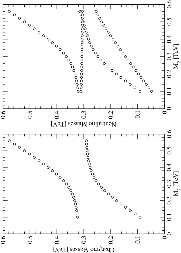
FIG. 2.: Variable $M_{2}$: chargino and neutralino masses. Here $\tan\beta=20$.

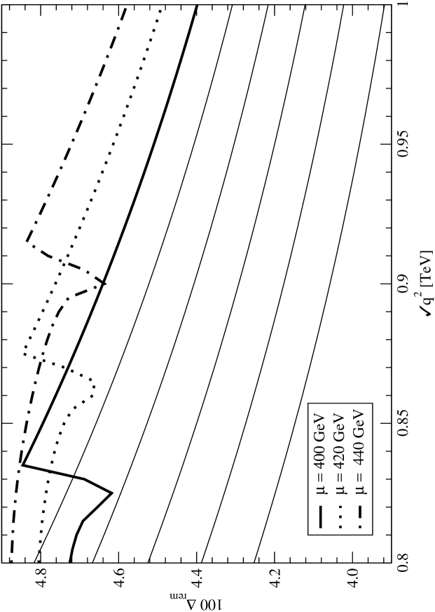
FIG. 3.: Variable $\mu$: plot of $\Delta_{\rm rem}$ for various $\mu$. The bottom curve has $\mu=300$ GeV. The other curves have increasing $\mu$ by steps of 20 GeV.

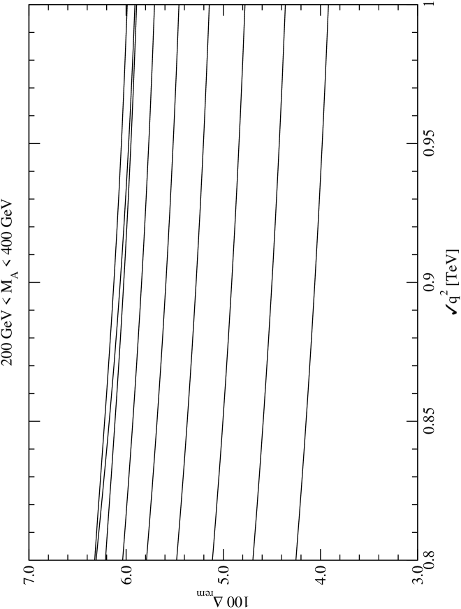
FIG. 4.: Variable $M_{A}$: plot of $\Delta_{\rm rem}$ for various $M_{A}$. The bottom line has $M_{A}=200$ GeV. The other curves have increasing $M_{A}$ by steps of 20 GeV.

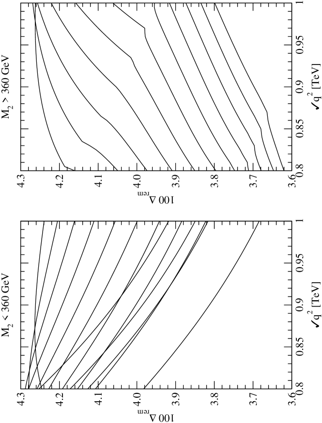
FIG. 5.: Variable $M_{2}$: plot of $\Delta_{\rm rem}$ for various $M_{2}$ between 100 and 560 GeV. The various curves have values of $M_{2}$ spaced by 20 GeV.

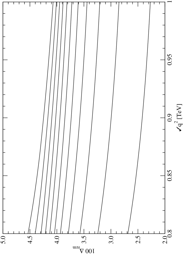
FIG. 6.: Variable $M_{S}$: plot of $\Delta_{\rm rem}$ for various $M_{S}$ between 100 and 400 GeV. The bottom line has $M_{S}=100$ GeV. The other curves have increasing $M_{S}$ by steps of 20 GeV.

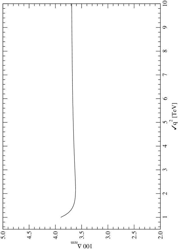
FIG. 7.: Behaviour of $\Delta_{\rm rem}$ in the ultra high energy regime.

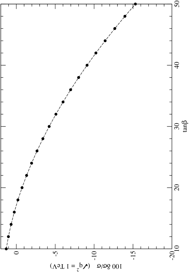
FIG. 8.: Variable $\tan\beta$ in the (L) scenario: full effect at 1 TeV

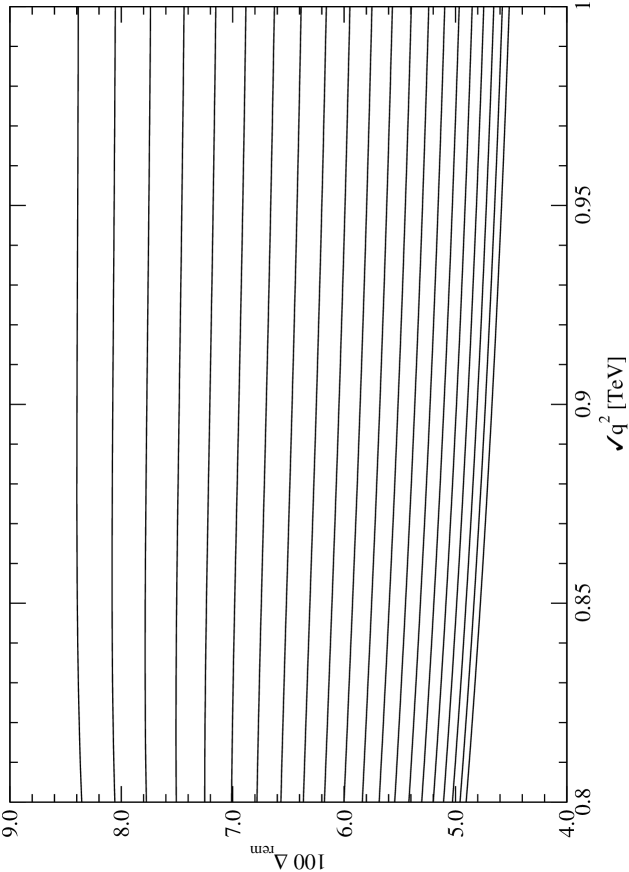
FIG. 9.: Variable $\tan\beta$ in the (L) scenario: $\Delta_{\rm rem}$. The bottom line has $\tan\beta=10$, the other curves have increasing $\tan\beta$ by steps $\Delta\tan\beta=2$.

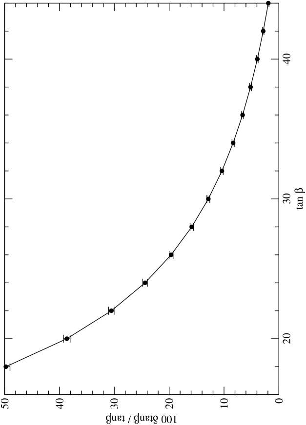
FIG. 10.: Variable $\tan\beta$ in the (L) scenario: percentual relative error in the determination of $\tan\beta$ at various $\tan\beta$.

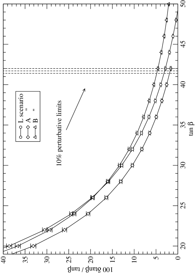
FIG. 11.: Variable $\tan\beta$ in the (L,A,B) scenarios: percentual relative error in the determination of $\tan\beta$ at various $\tan\beta$.

FIG. 12.: Contour plot of $100\Delta_{\rm rem}(1TeV)$ in the plane $(M_{A},M_{S})$. The contour lines correspond to values between 0 and 8.5 increasing from left to right by steps of 0.5. Also shown are the boxes corresponding to the points $(M_{A},M_{S})=(250\pm 5\ \mbox{GeV},330\pm 5\ \mbox{GeV})$ and $(M_{A},M_{S})=(330\pm 5\ \mbox{GeV},250\pm 5\ \mbox{GeV})$.

FIG. 13.: Surface plot of $100\Delta_{\rm rem}$ at 1 TeV in the plane $(M_{A},M_{S})$.

REFERENCES

- [1] see e.g., E. Accomando et.al., Phys. Rep. C299,299(1998).
- [2] ” The CLIC study of a multi-TeV linear collider”, CERN-PS-99-005-LP (1999).
- [3] M. Kuroda, G. Moultaka and D. Schildknecht, Nucl. Phys. B350,25(1991); G.Degrassi and A Sirlin, Phys.Rev. D46,3104(1992); W. Beenakker et al, Nucl. Phys. B410, 245 (1993), Phys. Lett. B317, 622 (1993); A. Denner, S. Dittmaier and R. Schuster, Nucl. Phys. B452, 80 (1995); A. Denner, S. Dittmaier and T. Hahn, Phys. Rev. D56, 117 (1997); P. Ciafaloni and D. Comelli, Phys. Lett. B446, 278 (1999); A. Denner, S.Pozzorini; Eur. Phys. J. C18, 461 (2001); Eur.Phys.J. C21, 63 (2001).
- [4] M. Beccaria, P. Ciafaloni, D. Comelli, F. Renard, C. Verzegnassi, Phys.Rev. D 61,073005 (2000); Phys.Rev. D 61,011301 (2000).
- [5] M. Beccaria, F.M. Renard and C. Verzegnassi, Phys. Rev. D63, 095010 (2001); Phys.Rev.D63, 053013 (2001);
- [6] V. V. Sudakov, Sov. Phys. JETP 3, 65 (1956); Landau-Lifshits: Relativistic Quantum Field theory IV tome (MIR, Moscow) 1972.
- [7] M. Ciafaloni, P. Ciafaloni and D. Comelli, Nucl. Phys. B589, 4810 (2000); V. S. Fadin, L. N. Lipatov, A. D. Martin and M. Melles, Phys. Rev. D61, 094002 (2000); J. H. Kühn, A. A. Penin and V. A. Smirnov, Eur. Phys. J C17, 97 (2000); J. H. Kühn, S. Moch, A. A. Penin and V. A. Smirnov, Nucl. Phys. B616, 286 (2001). M. Melles, Eur. Phys. J. C24,193(2002). M. Melles Phys. Rev. D63, 034003 (2001); Phys. Rev. D64, 014011 (2001), Phys. Rev. D64, 054003 (2001).
- [8] M. Melles, Electroweak radiative corrections in high-energy processes, hep-ph/0104232;
- [9] M. Beccaria, F. M. Renard and C. Verzegnassi, Phys. Rev. D64, 073008 (2001).
- [10] M. Beccaria, M. Melles, F. M. Renard and C. Verzegnassi, Phys.Rev.D65, 093007 (2002).
- [11] M. Beccaria, S. Prelovsek, F. M. Renard, C. Verzegnassi, Phys. Rev. D64, 053016 (2001).
- [12] The SESAMO code can be requested by contacting the authors at the e-mail address matteo.beccaria@le.infn.it.
- [13] See e.g. W. Hollik, in ”Precision Tests of the Standard Electroweak Model”, edited by P. Langacker (1993) p.37; MPI-Ph-93-021, BI-TP-93-16.
- [14] J. Guasch, W. Hollik, and A. Kraft, Nucl. Phys. B596, 66 (2001). The list of diagrams can be found on the WWW page http://www.hep-processes.de/.
- [15] G. Degrassi and A. Sirlin, Nucl. Phys. B383, 73 (1992); Phys. Rev. D46, 3104 (1992).
- [16] S. Heinemeyer, W. Hollik, G. Weiglein, Eur. Phys. J. C9 (1999) 343-366. See also the WWW page http://www-itp.physik.uni-karlsruhe.de/feynhiggs/ .
- [17] A. Datta, A. Djouadi and J.-L. Kneur, Phys. Lett. B509, 299 (2001).