1 Introduction

In this letter we make the observation that, at leading power in the mass of the $B$-meson ($M_{B}$), the nonperturbative QCD effects in the radiative $B$-decays, ${B\to\gamma\ell\nu_{\ell}}$, $B\to\gamma\ell^{+}\ell^{-}$ and $B\to\gamma\gamma$ are universal. By this we mean that, for the same photon energy $E_{\gamma}$, the amplitudes for the processes ${B\to\gamma\ell\nu_{\ell}}$ and $B\to\gamma\ell^{+}\ell^{-}$ are proportional to each other. For $E_{\gamma}=M_{B}/2$ they are also proportional to the amplitude for $B\to\gamma\gamma$. The constants of proportionality contain kinematic factors, CKM-matrix elements and a series in $\alpha_{s}(M_{B})$ which is therefore calculable in perturbation theory. Thus, in spite of the different weak-decay mechanisms for the three processes, the strong interaction effects are common at scales below $M_{B}$.

In ref. [1] we showed that the two form factors ($F_{A,V}$) for the ${B\to\gamma\ell\nu_{\ell}}$ decay are given, up to one-loop order, by the factorization formula:

$$F_{A,V}(E_{\gamma})=\int d\tilde{k}_{+}\Phi_{+}^{B}(\tilde{k}_{+};\mu_{F})\,T(\tilde{k}_{+},E_{\gamma};\mu_{F})\,,$$ (1)

with

$$T(\tilde{k}_{+},E_{\gamma};\mu_{F})=\left\{C_{3}^{SCET}(\mu_{F})\,\frac{f_{B}Q_{u}M_{B}}{2\sqrt{2}E_{\gamma}}\right\}\frac{1}{\tilde{k}_{+}}\left[1+\frac{\alpha_{s}(\mu_{F})C_{F}}{4\pi}\,K_{t}(\tilde{k}_{+},E_{\gamma};\mu_{F})\right],$$ (2)

where the momentum of the photon is in the $-$ direction, $C_{3}^{SCET}(\mu_{F})$ is a Wilson coefficient relating the weak $b\to u$ current to operators of the Soft-Collinear Effective Theory (SCET) [2], $f_{B}$ is the $B$-meson’s leptonic decay constant and $Q_{u}=-2/3$ is the charge of the $\bar{u}$-quark . $\mu_{F}$ is a factorization scale and is conveniently chosen to be $O(\sqrt{M_{B}\Lambda_{\textrm{\scriptsize{QCD}}}})$. The $B$-meson’s light-cone distribution amplitude, $\Phi_{+}^{B}$, is the component of the non-local matrix element [4, 5]

$$\Phi^{H}_{\alpha\beta}(\tilde{k}_{+})=\int dz_{-}e^{i\tilde{k}_{+}z_{-}}\left.\langle 0|\bar{u}_{\beta}(z)[z,0]b_{\alpha}(0)|H\rangle\right|_{z_{+},z_{\perp}=0}\,,$$ (3)

with the hadronic initial state $H=B$, which contributes to the amplitudes at leading twist. In eq. (3), $\alpha,\beta$ are spinor labels and $[z,0]$ denotes a path-ordered exponential. Finally,

$$K_{t}(\tilde{k}_{+},E_{\gamma};\mu_{F})=\log^{2}\frac{2\sqrt{2}E_{\gamma}\tilde{k}_{+}}{\mu_{F}^{2}}-\frac{\pi^{2}}{6}-1\,.$$ (4)

The above formulae hold for photon energies satisfying $E_{\gamma}\gg\Lambda_{\textrm{\scriptsize{QCD}}}$.

The nonperturbative contribution to the form factors is contained in $\Phi_{+}^{B}(\tilde{k}_{+})$ which is convoluted with $T$ as in eq. (1). The observation we make here is that precisely the same convolution over $\tilde{k}_{+}$ appears also in the amplitudes for $B\to\gamma\ell^{+}\ell^{-}$ and $B\to\gamma\gamma$ decays. The $\tilde{k}_{+}$-independent prefactor in curly brackets in eq. (2) is process-dependent but perturbative. Moreover, although the coefficient $C_{3}^{SCET}(\mu_{F})$ in eq. (2) is specific to the decay ${B\to\gamma\ell\nu_{\ell}}$, the behaviour with $\mu_{F}$ (for $\mu_{F}<m_{B}$) is common to all coefficients $C_{i}^{SCET}$ appearing in the three radiative decays. Thus ratios of amplitudes for different processes but with the same $E_{\gamma}$ only depend on the $C_{i}^{SCET}$ at $\mu_{F}=M_{B}$, and are hence calculable as perturbative series in $\alpha_{s}(M_{B})$. The formulae for the decay rates are presented explicitly in sec.3.

Additional motivation for this study is provided by the need to understand nonperturbative QCD effects in two-body exclusive nonleptonic decays, for which there is a wealth of experimental data, particularly from the $B$-factories. The demonstration of the factorization of long-distance effects at leading twist for these processes [6, 7, 8] provides the theoretical framework for detailed phenomenological analyses. However, our ignorance of $\Phi_{+}^{B}$ (and the lack of a similar framework for higher-twist contributions) limits the precision with which information about the CKM matrix elements and CP-violation can be determined from the experimental measurements of branching ratios and asymmetries. It is therefore important to understand whether there are relations, similar to those presented here, also between different nonleptonic decay amplitudes (or between contributions to the amplitudes) which reduce or eliminate the need for a detailed knowledge of $\Phi_{+}^{B}$. Finally we repeat that measuring the photon’s energy distribution in ${B\to\gamma\ell\nu_{\ell}}$ decays may in future be the best way of obtaining information about $\Phi_{+}^{B}$ [1].

In the next section we sketch the evaluation of the amplitudes for $B\to\gamma\gamma$ and $B\to\gamma\ell^{+}\ell^{-}$ decays at one-loop order and the resummation of the large logarithms. We focus on the differences with the corresponding calculation of the ${B\to\gamma\ell\nu_{\ell}}$ decay amplitude, which was described in detail in ref. [1]. The reader who is only interested in the implications of our results can turn immediately to section 3 where we present the expressions for the decay rates and discuss their significance.

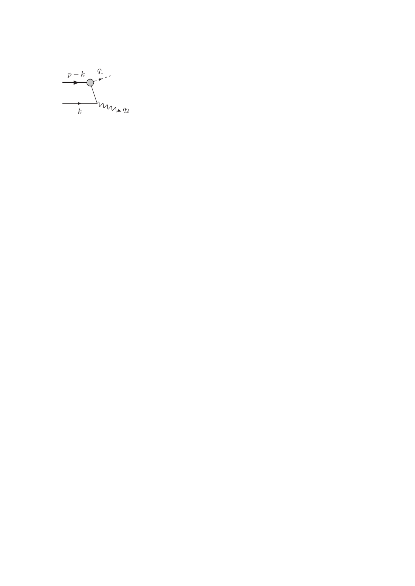
Figure 1: Lowest-order diagram at leading twist contributing to the process $b\bar{u}\to\gamma X$, where $X=\ell\nu_{\ell}$, $\ell^{+}\ell^{-}$ or $\gamma$ and is represented by the dashed line. The thick line represents the $b$-quark and the thin line a light quark. The grey circle represents the operator responsible for the $b\to u$ transition.

2 Amplitudes up to One-Loop Order

In ref. [1] we have described the evaluation of the one-loop contribution to the hard-scattering kernel for the decay ${B\to\gamma\ell\nu_{\ell}}$ in detail. The corresponding calculation for the other radiative decays is very similar, so here we only sketch the main points and present the results.

We wish to write the form factors for each of the three radiative processes in the generic factorized form given in eq. (1), where the hard-scattering kernel $T$ depends on the process, but, as its name suggests, does not depend on scales below $\mu_{F}$ and can be calculated in perturbation theory. In order to determine $T$ we are free to choose any appropriate and convenient external state, and we take a $u$-antiquark with momentum $k$ and a $b$-quark with momentum $p$ – $k$. The leading-twist contributions are those in which the photon is emitted from the light quark, and we will see that the diagrams which need to be evaluated are those in figs. 1 and 2.

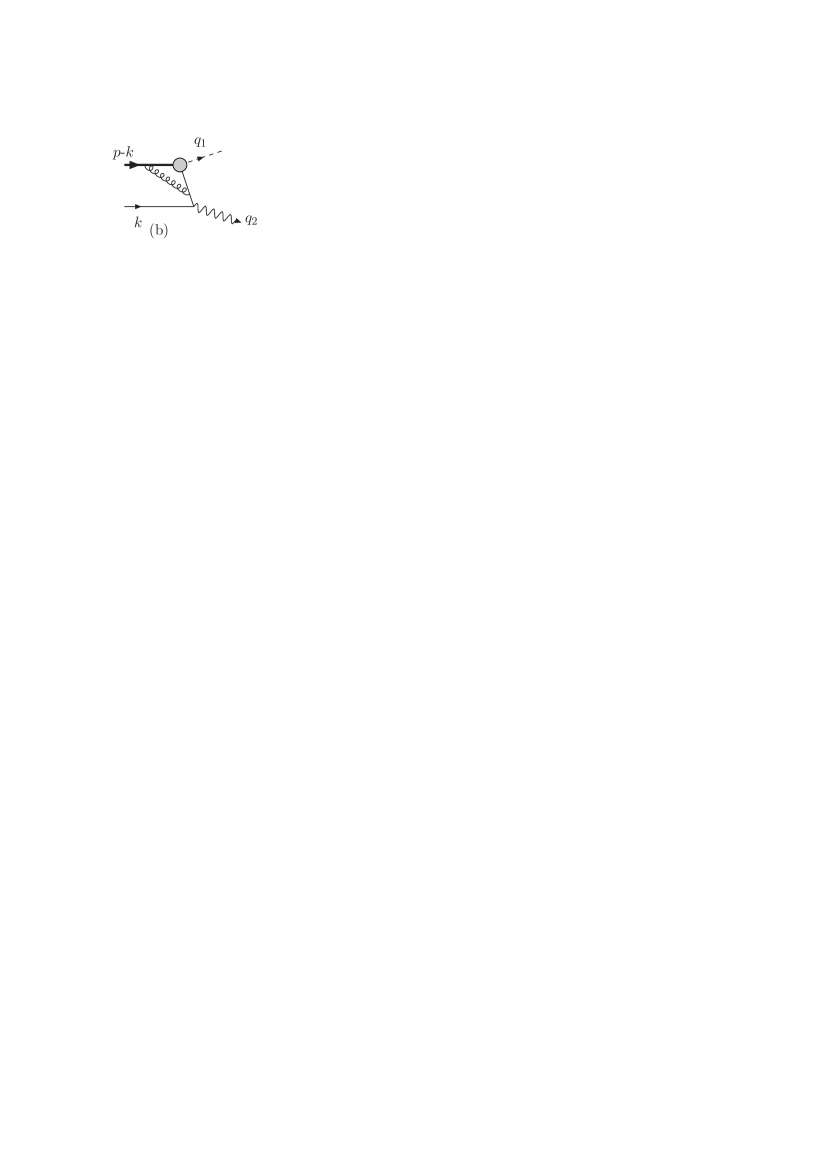
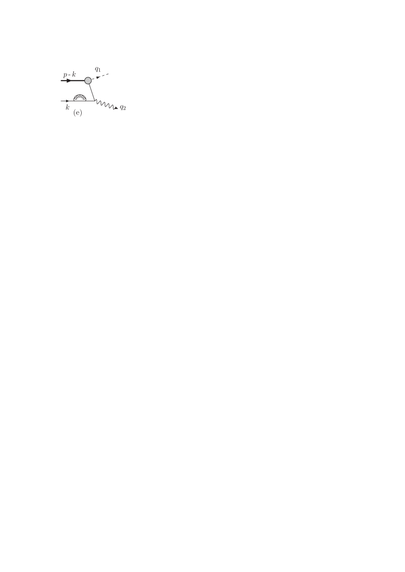
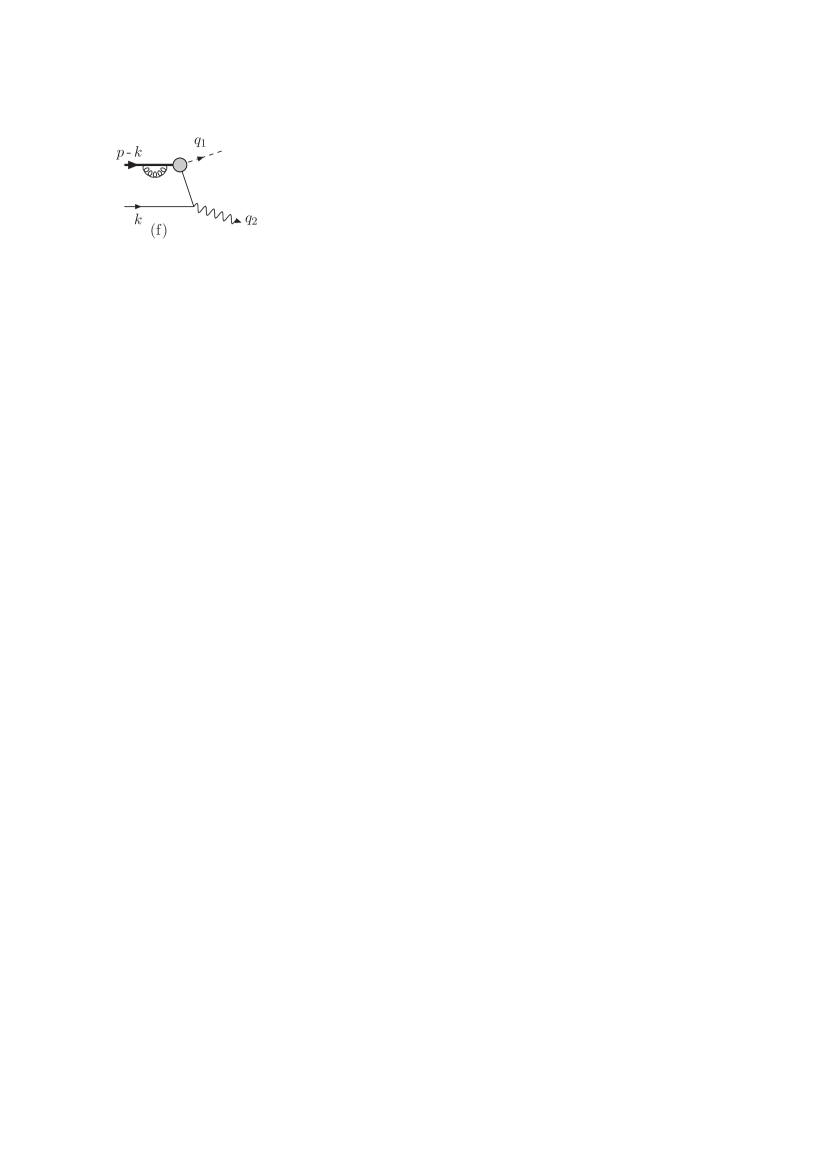
Figure 2: One-loop leading-twist diagrams for the process $b\bar{u}\to X\gamma$.

The evaluation of the one-loop graphs in fig. 2(a), (d), (e) and (f) is common to all the processes and is described in ref. [1]. In ref. [1] we also show that the leading-twist contribution from the box diagram in fig. 2(c) comes from the soft region of phase-space and is absorbed into the one-loop component of the wave-function, giving no contribution to $T$. This is also true for $B\to\gamma\gamma$ and $B\to\gamma\ell^{+}\ell^{-}$ decays. Thus in the following we present the results for the diagrams in fig. 1 and 2(b) for $B\to\gamma\gamma$ and $B\to\gamma\ell^{+}\ell^{-}$ decays and combine them with those in ref. [1] for the other graphs (the graphs are evaluated in the Feynman gauge).

2.1 The decay $B\to\gamma\gamma$

The effective Hamiltonian for $B_{q}^{0}\to\gamma\gamma$ decays is [9, 10]

$${\mathcal{H}}=i\lambda_{t}^{(q)}\frac{eG_{F}}{4\pi^{2}\sqrt{2}}m_{b}C_{7}^{\rm{eff}}(\mu_{R})\,[\bar{q}\gamma^{\mu}\gamma^{\nu}b_{R}](\partial_{\mu}A_{\nu}-\partial_{\nu}A_{\mu})\,,$$ (5)

where $b_{R}=1/2(1+\gamma_{5})b$, $q=d$ or $s$ and $\lambda_{t}^{(q)}=V^{*}_{tq}V_{tb}$. $C_{7}^{\rm{eff}}$ is the Wilson coefficient at the scale $\mu_{R}$ (it will generally be convenient to take $\mu_{R}=M_{B}$). The superscript eff denotes the fact that $C_{7}^{\rm{eff}}$ contains terms proportional to the Wilson coefficients $C_{1\textrm{\,--\,}6}$ (corresponding to $\Delta B=1$ four-quark operators) and $C_{8}$ (corresponding to the chromomagnetic operator). The contributions included in $C_{7}^{\rm{eff}}$ are short-distance loop corrections to $O_{1\,\textrm{--}\,6}$ and $O_{8}$ which result in an effective vertex proportional to the operator $O_{7}$ at tree-level (i.e. to the operator in eq. (5)).

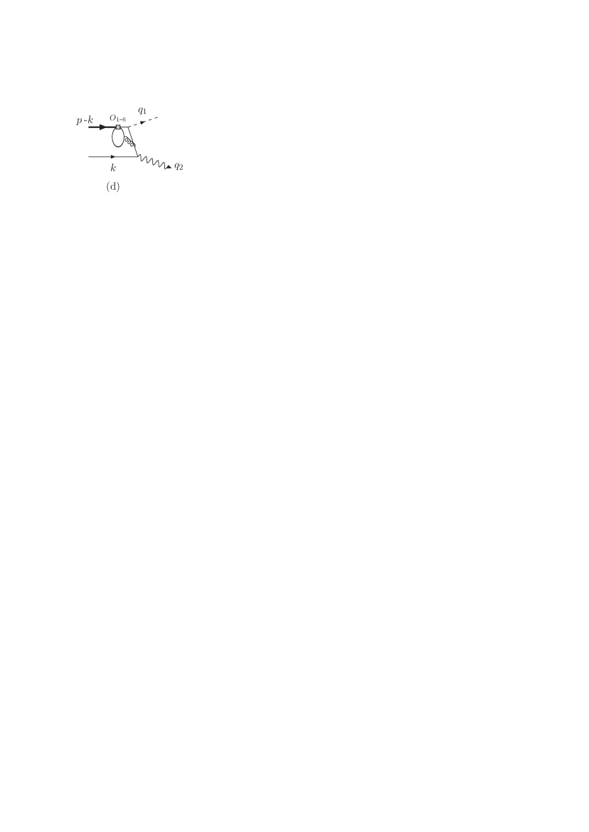
Figure 3: Sample diagrams which contribute to $C_{7}^{\rm{eff}}$ ((a) – (d)). The non-factorizable diagram (e) does not contribute at leading twist.

We now briefly illustrate how the leading-twist contributions proportional to $C_{1\textrm{\,--\,}6}$ and $C_{8}$ are absorbed into $C_{7}^{\rm{eff}}$. It is not surprising that the diagram in fig 3(a) has the structure of fig. 1, where the grey circle represents the electromagnetic operator $O_{7}$, and its contribution can therefore be included into $C_{7}^{\rm{eff}}$. Indeed this is conventionally done [9]. In fig. 3(b), (c) and (d) we draw, for illustration, three diagrams at $O(\alpha_{s})$ contributing to $C_{7}^{\rm{eff}}$. The key point to note is that the loop integrations are dominated by the short-distance region of phase space, and therefore the contributions to $C_{7}^{\rm{eff}}$ are calculable in perturbation theory. In fact $C_{7}^{\rm{eff}}$ at $O(\alpha_{s})$ can be deduced from the calculations in refs. [11, 12] (for the penguin operators $O_{3\textrm{\,--\,}6}$, for which the Wilson coefficients are small, the contribution to $C_{7}^{\rm{eff}}$ is only known at $O(\alpha_{s}^{0})$). In the basis and notation of refs [11, 12]

$$C_{7}^{\rm{eff}}=C_{7}-\frac{C_{3}}{3}-\frac{4C_{4}}{9}-\frac{20\,C_{5}}{3}-\frac{80\,C_{6}}{9}-\frac{\alpha_{s}}{4\pi}\sum_{1,2,8}C_{i}F_{i}^{(7)}\,,$$ (6)

where $F_{1,2}^{(7)}$ and $F_{8}^{(7)}$ are given in eq. (56) of ref. [11] and eq. (82) of ref. [12] respectively. There are other contributions proportional to $C_{1\textrm{\,--\,}6}$ and $C_{8}$ which cannot be absorbed into $C_{7}^{\rm{eff}}$. An example is drawn in fig. 3(e). However, power-counting arguments show that these contributions are suppressed by at least one power of $M_{B}$. The contributions to the hard-scattering kernel from the $O(\alpha_{s})$ diagrams drawn in fig. 2, where the grey circle represents the tree-level insertion of $O_{7}$, are evaluated explicitly in this letter.

The amplitude (${\cal A}$) for the decay $B\to\gamma\gamma$ can be written in terms of invariant form factors $A_{\pm}$:

$${\mathcal{A}}(B\to\gamma\gamma)=\frac{\alpha G_{F}f_{B}}{3\pi\sqrt{2}}\Big{\{}2A_{-}\,\varepsilon(q_{1},q_{2},\epsilon^{*}_{1},\epsilon^{*}_{2})+A_{+}\,\left[\,2i(q_{1}\cdot\epsilon^{*}_{2})(q_{2}\cdot\epsilon^{*}_{1})-iM_{B}^{2}(\epsilon^{*}_{1}\cdot\epsilon^{*}_{2})\,\right]\Big{\}}.$$ (7)

Following ref. [1], we choose the external state $H=b\bar{q}$ to determine the contribution to the hard-scattering kernel. We denote the contribution from the tree diagram in fig. 1, where the photon with momentum $q_{1}$ is emitted from the effective vertex, to the $\langle\gamma\gamma|{\cal H}|b\bar{q}\rangle$ matrix element by $F_{1}^{(0)}$ (0 denotes tree-level or “zero loops”). Similarly $F_{2}^{(0)}$ is the contribution with the photon with momentum $q_{2}$ emitted from the effective vertex, and is equal to $F_{1}^{(0)}$ with the obvious replacements $1\leftrightarrow 2$ and $+\leftrightarrow-$ in the expressions below.

Evaluating the diagram we find for the matrix element at tree level

$$F_{1}^{(0)}=\lambda_{t}^{(q)}\frac{eG_{F}}{8\pi^{2}\sqrt{2}}m_{b}C_{7}^{\rm{eff}}\cdot\frac{e_{q}}{\sqrt{2}M_{B}k_{+}}\bar{v}^{s}(k)\left[\epsilon\hbox to0.0pt{\hss/}_{2}^{*}q\hbox to0.0pt{\hss/}_{2}[q\hbox to0.0pt{\hss/}_{1},\epsilon\hbox to0.0pt{\hss/}_{1}^{*}](1+\gamma_{5})\right]u^{S}(p-k),$$ (8)

where $u$ and $v$ are the wave functions of the $b$ and $\bar{q}$ quarks with spin labels $S$ and $s$. Writing this amplitude as a convolution

$$F_{1}^{(0)}=\int\frac{d\tilde{k}_{+}}{2\pi}\Phi^{b\bar{q}\,(0)}_{\alpha\beta}T_{1\,\beta\alpha}^{(0)}$$ (9)

(with $\Phi^{b\bar{q}}$ defined in eq. (3) with $H=b\bar{q}$), the contribution to the hard-scattering kernel is

$$T_{1\,\beta\alpha}^{(0)}=\lambda_{t}^{(q)}\frac{eG_{F}}{8\pi^{2}\sqrt{2}}m_{b}C_{7}^{\rm{eff}}\cdot\frac{e_{q}}{\sqrt{2}M_{B}\tilde{k}_{+}}\left[\epsilon\hbox to0.0pt{\hss/}_{2}^{*}q\hbox to0.0pt{\hss/}_{2}[q\hbox to0.0pt{\hss/}_{1},\epsilon\hbox to0.0pt{\hss/}_{1}^{*}](1+\gamma_{5})\right]_{\beta\alpha}\,.$$ (10)

Adding the contribution from $T_{2\,\beta\alpha}^{(0)}$, we obtain for the lowest-order contribution to the two form factors:

$$A_{+} = A_{-}=\int d\tilde{k}_{+}\Phi_{+}^{B}(\tilde{k}_{+};\mu_{F})T^{(0)}(\tilde{k}_{+};\mu_{R},\mu_{F})=\lambda_{t}^{(q)}C_{7}^{\rm{eff}}(\mu_{R})\frac{M_{B}}{\lambda_{B}}\,,$$ (11)

$$T^{(0)} = C_{7}^{\rm{eff}}(\mu_{R})\frac{\lambda_{t}^{(q)}M_{B}}{\sqrt{2}\tilde{k}_{+}}\,,\qquad\frac{1}{\lambda_{B}}=\frac{1}{\sqrt{2}}\int\,d\tilde{k}_{\pm}\,\frac{\Phi_{+}^{B}(\tilde{k}_{\pm})}{\tilde{k}_{\pm}}\,.$$ (12)

Note that $\lambda_{B}$ is also the nonperturbative quantity which is needed in evaluating the contribution from tree-level hard-spectator interactions to exclusive nonleptonic $B$-decay amplitudes [6, 7, 8].

At one-loop order, the contribution of the diagram in fig. 2(b) to the $\langle\gamma\gamma|{\cal H}|b\bar{u}\rangle$ matrix element is

$$F_{1}^{(1)\,\textrm{\scriptsize wk}}=F_{1}^{(0)}\frac{\alpha_{s}C_{F}}{4\pi}\left[-\log^{2}\frac{\sqrt{2}k_{+}}{M_{B}}-2\log\frac{\sqrt{2}k_{+}}{M_{B}}-\pi^{2}\right].$$ (13)

In order to determine the one-loop contribution to $T$ ($T^{(1)}$), we need to subtract the corresponding contribution to $\Phi^{b\bar{q}\,(1)}\otimes T^{(0)}$, the convolution of the one-loop component of $\Phi^{b\bar{u}}$ with $T^{(0)}$:

$$\left(\Phi^{(1)\,\textrm{\scriptsize wk}}\otimes T^{(0)}\right)_{1}=F_{1}^{(0)}\cdot\frac{\alpha_{s}C_{F}}{4\pi}\left[-\frac{4}{\omega^{2}}+\frac{2}{\omega}\log\frac{2k_{+}^{2}}{\mu_{F}^{2}}-2\log^{2}\frac{\sqrt{2}k_{+}}{\mu_{F}}-\frac{3\pi^{2}}{4}\right]\,,$$ (14)

where we use dimensional regularization, working in $4-\omega$ dimensions. We recall that the subscript 1 denotes the contribution from the graphs with the photon of momentum $q_{1}$ emitted from the effective vertex.

The contribution to the hard-scattering kernel from the diagram in fig. 2(b) with $q_{1}\leftrightarrow q_{2}$ is the same, since the resulting convolution over $\tilde{k}_{-}$ is equal by symmetry to the one over $\tilde{k}_{+}$ from fig. 2(b). We therefore present our answers below in terms of a convolution with $\tilde{k}_{+}$ as the (dummy) integration variable, and our expressions for the hard-scattering kernel correspond to the sum of the two contributions.

The results in eqs. (13) and (14), together with those in ref. [1] for the remaining diagrams in fig. 2 can be combined to give the one-loop expression for the hard-scattering kernel:

$$T = T^{(0)}\Bigg{[}1+\frac{\alpha_{s}C_{F}}{4\pi}\Bigg{(}\log^{2}\frac{\sqrt{2}\tilde{k}_{+}}{M}+4\log\frac{\sqrt{2}\tilde{k}_{+}}{M}\log\frac{M}{\mu_{F}}$$ (15)

$$+2\log^{2}\frac{M}{\mu_{F}}+7\log\frac{M}{\mu_{F}}-2\log\frac{\mu_{R}}{\mu_{F}}-7-\frac{\pi^{2}}{4}\Bigg{)}\Bigg{]}\,,$$

where the explicit expression for $T^{(0)}$ is given in eq. (12).

We now use the SCET formalism to resum the large logarithms following the steps in sec. 5 of ref. [1]. The contribution of the tensor operator to the $\langle\gamma\gamma|{\cal H}|b\bar{u}\rangle$ matrix element (i.e. the diagrams in figs. 1 and 2(b) plus half of the diagrams in figs. 2(d) and 2(e)) is

$$F^{J_{W}}=F_{1}^{(0)}\Bigg{\{}1+\frac{\alpha_{s}C_{F}}{4\pi}\left[2\log\frac{M_{B}}{\mu_{R}}-\log^{2}\frac{\sqrt{2}k_{+}}{M_{B}}-\frac{7}{2}\log\frac{\sqrt{2}k_{+}}{M_{B}}-\frac{5}{2}-\pi^{2}\right]\bigg{\}}$$

$$+F_{2}^{(0)}\bigg{\{}1+\frac{\alpha_{s}C_{F}}{4\pi}\left[2\log\frac{M_{B}}{\mu_{R}}-\log^{2}\frac{\sqrt{2}k_{-}}{M_{B}}-\frac{7}{2}\log\frac{\sqrt{2}k_{-}}{M_{B}}-\frac{5}{2}-\pi^{2}\right]\Bigg{\}}\,.$$ (16)

In the SCET formalism, only one operator, denoted by $O_{9}$ in ref. [2], contributes to the form factors. From eq. (66) of ref. [1] and the neighbouring discussion, we can rewrite $F^{J_{W}}$ in terms of the SCET Wilson coefficient $C_{9}^{SCET}(E_{\gamma};\mu_{R},\mu_{F})$ as

$$F^{J_{W}} = C^{SCET}_{9}\!\big{(}M_{B}/2;\mu_{R},M_{B}\big{)}\times$$ (17)

$$\Bigg{\{}F_{1}^{(0)}\bigg{(}1+\frac{\alpha_{s}C_{F}}{4\pi}\big{[}-\log^{2}\frac{\sqrt{2}k_{+}}{M_{B}}-\frac{7}{2}\log\frac{\sqrt{2}k_{+}}{M_{B}}+\frac{7}{2}-\frac{11\pi^{2}}{12}\big{]}\bigg{)}$$

$$+F_{2}^{(0)}\bigg{(}1+\frac{\alpha_{s}C_{F}}{4\pi}\big{[}-\log^{2}\frac{\sqrt{2}k_{-}}{M_{B}}-\frac{7}{2}\log\frac{\sqrt{2}k_{-}}{M_{B}}+\frac{7}{2}-\frac{11\pi^{2}}{12}\big{]}\bigg{)}\Bigg{\}}\,.$$

Comparing eqs. (16) and (17) we find

$$C_{9}^{SCET}(\frac{M_{B}}{2};\mu_{R},M_{B})=1+\frac{\alpha_{s}C_{F}}{4\pi}\left[2\log\frac{M_{B}}{\mu_{R}}-6-\frac{\pi^{2}}{12}\right]\,,$$ (18)

which agrees with eq. (33) of ref. [2] for $\mu_{R}=M_{B}$.

Finally, we can use the renormalization group equation for $C_{9}^{SCET}$, derived in ref. [2], to obtain its value at any factorization scale $\mu_{F}$. We conclude that the form factors $A_{+}=A_{-}$ are given by the generic form in eq. (1) with

$$T(\tilde{k}_{+};\mu_{R},\mu_{F})=\frac{\lambda_{t}^{(q)}M_{B}}{\sqrt{2}\tilde{k}_{+}}\,C_{7}^{\rm{eff}}(\mu_{R})\,C^{SCET}_{9}(M_{B}/2\hskip 2.0pt;\mu_{R},\mu_{F})\,\left[1+\frac{\alpha_{s}C_{F}}{4\pi}K_{t}\big{(}\tilde{k}_{+},M_{B}/2;\mu_{F}\big{)}\right].$$ (19)

Thus the hard-scattering kernel has exactly the same dependence on $\tilde{k}_{+}$ as that for ${B\to\gamma\ell\nu_{\ell}}$ decays in eq. (2).

2.2 The decay $B\to\gamma\ell^{+}\ell^{-}$

The procedure for the evaluation of the $B\to\gamma\ell^{+}\ell^{-}$ decay amplitude follows exactly the same steps. We will assume here that $x_{\gamma}\equiv 2E_{\gamma}/M_{B}$ satisfies $(1-x_{\gamma})\gg\Lambda_{\textrm{\scriptsize{QCD}}}/M_{B}$. This allows us to neglect the diagrams in which the real photon is emitted from the weak vertex and the virtual one is radiated from the light quark. The effective Hamiltonian for this process is then [9, 13, 14]:

$${\mathcal{H}}=\lambda_{t}^{(q)}\frac{\alpha G_{F}}{\pi\sqrt{2}}\bigg{(}C_{9}^{\rm eff}(\bar{q}\gamma_{\mu}b_{L})(\bar{\ell}\gamma^{\mu}\ell)+C_{10}(\bar{q}\gamma_{\mu}b_{L})(\bar{\ell}\gamma^{\mu}\gamma_{5}\ell)-2\frac{C_{7}^{\rm{eff}}}{q_{1}^{2}}m_{b}(\bar{q}i\sigma_{\mu\nu}q_{1}^{\nu}b_{R})(\bar{\ell}\gamma^{\mu}\ell)\bigg{)}\,,$$ (20)

where $b_{L,R}=(1\mp\gamma_{5})/2\,b$. Again $C_{9}^{\rm eff}$ contains short-distance, leading-twist contributions from four-quark and chromomagnetic operators:

$$C_{9}^{\rm eff}=C_{9}+Y(q_{1}^{2})-\frac{\alpha_{s}}{4\pi}\sum_{1,2,8}C_{i}F_{i}^{(9)}\,,$$ (21)

where $Y(q^{2}_{1})$ has contributions from $O_{1\textrm{\,--\,}6}$ and its explicit expression is given in eq. (10) of ref. [12] and $F_{1,2}^{(9)}$ and $F_{8}^{(9)}$ are given in eqs. (54) and (55) of ref. [11] and eq. (83) of ref. [12] respectively. We follow the authors of ref. [14] in neglecting the long-distance effects associated with $c\bar{c}$ resonances. For the purposes of this paper, we start with eq. (20) and evaluate the matrix elements of the operators on the right-hand side. The four form factors for this process are defined by:

$$2\langle\gamma(q,\epsilon^{*})|\bar{q}\gamma_{\mu}b_{L}|\bar{B}(p)\rangle=e\epsilon_{\mu\nu\rho\sigma}{\epsilon^{*}}^{\nu}v^{\rho}q^{\sigma}F_{V}(E_{\gamma})+ie[\epsilon^{*}_{\mu}(v\cdot q)-q_{\mu}(v\cdot\epsilon^{*})]F_{A}(E_{\gamma})$$ (22)

and

$$2\langle\gamma(q,\epsilon^{*})|\bar{q}i\sigma_{\mu\nu}(p-q)^{\nu}b_{R}|\bar{B}(p)\rangle = -eM_{B}\epsilon_{\mu\nu\rho\sigma}{\epsilon^{*}}^{\nu}v^{\rho}q^{\sigma}F_{T}(E_{\gamma})$$ (23)

$$-ieM_{B}[\epsilon^{*}_{\mu}(v\cdot q)-q_{\mu}(v\cdot\epsilon^{*})]F^{\prime}_{T}(E_{\gamma})\,.$$

Since the corrections to the vector and axial currents have already been discussed in ref. [1], we consider here only the form factors $F_{T}$ and $F_{T}^{\prime}$. Evaluating the diagram in fig. 1 we find that at lowest order the contribution to the matrix element $2\langle\ell^{+}\ell^{-}\gamma|\bar{q}i\sigma_{\mu\nu}q_{1}^{\nu}b_{R}|b\bar{q}\rangle$ is

$$F^{(0)}_{\mu}=\frac{e_{q}}{2(q_{2})_{-}k_{+}}\,\bar{v}^{s}(k)\left[\epsilon\hbox to0.0pt{\hss/}^{*}q\hbox to0.0pt{\hss/}_{2}[\gamma_{\mu},q\hbox to0.0pt{\hss/}_{1}]\right]u^{S}_{R}(p-k)\,,$$ (24)

and the hard-scattering amplitude is

$$T^{(0)}_{\mu}=\frac{e_{q}}{4(q_{2})_{-}k_{+}}\left[\epsilon\hbox to0.0pt{\hss/}^{*}q\hbox to0.0pt{\hss/}_{2}[\gamma_{\mu},q\hbox to0.0pt{\hss/}_{1}](1+\gamma_{5})\right]_{\beta\alpha}\,.$$ (25)

The form factors at lowest order are thus given by

$$F_{T}=F^{\prime}_{T}=\frac{Q_{q}f_{B}M_{B}}{2E_{\gamma}\lambda_{B}}\,,$$ (26)

where $Q_{q}=1/3$ is the electric charge of $\bar{q}$.

At one-loop order the contribution from the diagram of fig. 2(b) to the matrix element $2\langle\ell^{+}\ell^{-}\gamma|\bar{q}i\sigma_{\mu\nu}q_{1}^{\nu}b_{R}|b\bar{q}\rangle$ is

$$F^{(1)\,\textrm{\scriptsize wk}}_{\mu}=F_{\mu}^{(0)}\cdot\frac{\alpha_{s}C_{F}}{4\pi}\Bigg{[}-\log^{2}\frac{z}{y}-2\log\frac{z}{y}-2\log\frac{z}{y}\log\frac{x}{y}-\log^{2}\frac{x}{y}-2{\rm Li}_{2}\left(1-\frac{y}{x}\right)-\pi^{2}\Bigg{]}\,,$$ (27)

where $x=M_{B}^{2}$, $y=2M_{B}E_{\gamma}$ and $z=2q_{2}\cdot k$. The corresponding contribution to $\Phi^{b\bar{q}\,(1)}\otimes T^{(0)}$ is given by the r.h.s. of eq. (14) with $F_{1}^{(0)}$ replaced by $F_{\mu}^{(0)}$ given in (24).

Combining the above results with the remaining diagrams in fig. 2 from ref. [1] we find that the hard-scattering kernel is given by

$$T_{\mu} = T_{\mu}^{(0)}\Bigg{[}1+\frac{\alpha_{s}C_{F}}{4\pi}\Big{(}\log^{2}\frac{z}{x}+2\log\frac{z}{x}\log\frac{x}{\mu_{F}^{2}}-2\log\frac{\mu_{F}^{2}}{y}-2\log^{2}\frac{x}{y}$$ (28)

$$\qquad+\frac{1}{2}\log^{2}\frac{x}{\mu_{F}^{2}}-2{\rm Li}_{2}\left(1-\frac{y}{x}\right)-\log\frac{\mu_{R}^{2}}{\mu_{F}^{2}}+\frac{3}{2}\log\frac{x}{\mu_{F}^{2}}-\frac{\pi^{2}}{4}-7\Big{)}\Bigg{]}\,.$$

We now perform the resummation of the large logarithms as for the $B\to\gamma\gamma$ decays above. By comparing our results for the contribution of the tensor operator to the matrix element $F^{J_{W}}$ with the results for the same transition in the SCET, we obtain the expression of $C_{9}^{SCET}(E_{\gamma};\mu_{R},\mu_{F}=M_{B})$ (it is given explicitly in eq. (33) below). For $\mu_{R}=M_{B}$ our result agrees with eq. (33) of ref. [2].

In this way we find that the form factors $F_{T}$ and $F_{T}^{\prime}$ are given by the generic form in eq. (1) with

$$T(\tilde{k}_{+},E_{\gamma};\mu_{R},\mu_{F})=\frac{f_{B}M_{B}}{6\sqrt{2}E_{\gamma}}\frac{1}{\tilde{k}_{+}}C^{SCET}_{9}(E_{\gamma};\mu_{R},\mu_{F})\left[1+\frac{\alpha_{s}C_{F}}{4\pi}K_{t}(\tilde{k}_{+},E_{\gamma};\mu_{F})\right]\,.$$ (29)

This completes the demonstration that at one-loop and leading-twist order the hard-scattering kernel has the same form for all three radiative decays.

3 Discussion and Conclusions

As a consequence of the universality of the nonperturbative effects in radiative $B$-decays the rates can be related simply using perturbation theory. The decay rates are given by the following expressions:

$$\Gamma(\bar{B}_{q}\to\gamma\gamma) = \frac{\alpha^{2}G_{F}^{2}M_{B}^{5}f_{B}^{2}}{144\pi^{3}}\,\left(C_{7}^{{\rm eff}}\right)^{2}\,|\lambda_{t}^{(q)}|^{2}(C^{SCET}_{9})^{2}\,\frac{1}{\Lambda_{B}^{2}(M_{B}/2)}\,,$$ (30)

$$\frac{d\Gamma(\bar{B}_{q}\to\gamma e^{+}e^{-})}{dE_{\gamma}} = \frac{\alpha^{3}G_{F}^{2}M_{B}^{4}f_{B}^{2}}{1728\pi^{4}}|\lambda^{(q)}_{t}|^{2}\,\frac{x_{\gamma}(1-x_{\gamma})}{\Lambda_{B}^{2}(E_{\gamma})}\times$$ (31)

$$\left[\Big{|}\,C_{9}^{\rm eff}\,C^{SCET}_{3}+\frac{2\,C_{7}^{\rm{eff}}}{1-x_{\gamma}}\,C^{SCET}_{9}\,\Big{|}^{2}+\left|\,C_{10}\,C^{SCET}_{3}\,\right|^{2}\right]\!,$$

$$\frac{d\Gamma(B^{+}\to\gamma e^{+}\nu)}{dE_{\gamma}} = \frac{\alpha G_{F}^{2}f_{B}^{2}|V_{ub}|^{2}M_{B}^{4}}{54\pi^{2}}(C^{SCET}_{3})^{2}\frac{x_{\gamma}(1-x_{\gamma})}{\Lambda_{B}^{2}(E_{\gamma})}\,,$$ (32)

where $x_{\gamma}=2E_{\gamma}/M_{B}$. $C_{3,9}^{SCET}$ in eqs. (30) - (32) denote the matching coefficients relating the QCD and SCET operators evaluated at $\mu_{F}=M_{B}$ and are calculable in perturbation theory,

$$C^{SCET}_{9}=1+\frac{\alpha_{s}(M_{B})C_{F}}{4\pi}\bigg{(}\log\frac{M_{B}^{2}}{\mu_{R}^{2}}-2\log^{2}x_{\gamma}+2\log x_{\gamma}-2{\rm Li}_{2}\left(1-x_{\gamma}\right)-6-\frac{\pi^{2}}{12}\bigg{)}$$ (33)

and

$$C^{SCET}_{3}=1+\frac{\alpha_{s}(M_{B})C_{F}}{4\pi}\bigg{(}-2\log^{2}x_{\gamma}-2{\rm Li}_{2}\left(1-x_{\gamma}\right)+\frac{3x_{\gamma}-2}{x_{\gamma}-1}\log x_{\gamma}-6-\frac{\pi^{2}}{12}\bigg{)}\,.$$ (34)

$\mu_{R}$ is the scale where the Wilson coefficient functions of the operators in the effective Hamiltonian, $C_{7}^{\rm{eff}},\,C_{9}^{\rm eff}$ and $C_{10}$, are evaluated, and for convenience we set $\mu_{R}=M_{B}$. The only nonperturbative parameter in eqs. (30) - (32) is $\Lambda_{B}(E_{\gamma})$, which is the generalization of $\lambda_{B}$:

$$\frac{1}{\Lambda_{B}(E_{\gamma})}=\frac{1}{\sqrt{2}}\exp[-S(E_{\gamma};\mu_{F})]\int d\tilde{k}_{+}\frac{\Phi_{+}^{B}(\tilde{k}_{+};\mu_{F})}{\tilde{k}_{+}}\left[1+\frac{\alpha_{s}C_{F}}{4\pi}\left(\log^{2}\frac{2\sqrt{2}E_{\gamma}\tilde{k}_{+}}{\mu_{F}^{2}}-\frac{\pi^{2}}{6}-1\right)\right]\,.$$ (35)

The resummation of large (Sudakov) logarithms is obtained through the evolution of SCET operators from $M_{B}$ down to $\mu_{F}$ (this evolution is common to all the operators), leading to the exponential factor in $\Lambda_{B}(E_{\gamma})$

$$-S(E_{\gamma};\mu_{F}) = \frac{f_{0}(r)}{\alpha_{s}(m_{b})}+f_{1}(r)\,,$$ (36)

$$f_{0}(r) = -\frac{4\pi C_{F}}{\beta^{2}_{0}}\left[\frac{1}{r}-1+\log r\right]\,,$$ (37)

$$f_{1}(r) = -\frac{C_{F}\beta_{1}}{\beta_{0}^{3}}\left[1-r+r\log r-\frac{\log^{2}r}{2}\right]$$ (38)

$$+\frac{C_{F}}{\beta_{0}}\left[\frac{5}{2}-2\log x_{\gamma}\right]\log r-\frac{2C_{F}B}{\beta_{0}^{2}}[r-1-\log r]\,,$$

where $r=\alpha_{s}(\mu_{F})/\alpha_{s}(m_{b})$, $\beta_{0}=11C_{A}/3-2N_{f}/3$ and $\beta_{1}=34C_{A}^{2}/3-10C_{A}N_{f}/3-2C_{F}N_{f}$.

In this letter we do not perform a detailed phenomenological analysis. For illustration however, in fig. 4 we plot the ratio

$$R_{q}(E_{\gamma})=\frac{d\Gamma(\bar{B}_{q}\to\gamma e^{+}e^{-})/dE_{\gamma}}{d\Gamma(B^{+}\to\gamma e^{+}\nu)/dE_{\gamma}}\,,$$ (39)

for $q=d,s$ and for the following values for the Wilson coefficients: $C_{7}^{\rm{eff}}=-0.390$, $C_{9}^{\rm eff}=4.182$ and $C_{10}=-4.234$ [9, 13, 14] (a more detailed analysis would include the effects of $Y(q_{1}^{2})$ and the $O(\alpha_{s})$ corrections to these coefficients, but these are sufficiently small to be neglected in this presentation). We take $|\lambda_{t}^{(d)}|=7.8\times 10^{-3}$, $|\lambda_{t}^{(s)}|=4.1\times 10^{-2}$, $|V_{ub}|=3.6\times 10^{-3}$, $f_{B_{d}}=190\,$MeV and $f_{B_{s}}=230\,$MeV. In other words we plot

$$R_{d}\times\left(\frac{7.8\times 10^{-3}}{|\lambda_{t}^{(d)}|}\right)^{2}\!\!\left(\frac{|V_{ub}|}{3.6\times 10^{-3}}\right)^{2}\!\!\left(\frac{f_{B_{d}}}{190\,\textrm{MeV}}\right)^{2}\qquad\textrm{and}$$ (40)

$$R_{s}\times\left(\frac{4.1\times 10^{-2}}{|\lambda_{t}^{(s)}|}\right)^{2}\!\!\left(\frac{|V_{ub}|}{3.6\times 10^{-3}}\right)^{2}\!\!\left(\frac{f_{B_{s}}}{230\,\textrm{MeV}}\right)^{2}\!\!.$$ (41)

The two curves are proportional to each other, differing by the values of the leptonic decay constants and CKM matrix elements. They do not depend however, on the model for the distribution amplitude. As $x_{\gamma}$ approaches 1 the virtual photon approaches its mass shell and this is the reason for the rise of the curves in this region. We recall however that our expressions are valid in the region $1-x_{\gamma}\gg\Lambda_{\textrm{\scriptsize{QCD}}}/M_{B}$ (and $x_{\gamma}\gg\Lambda_{\textrm{\scriptsize{QCD}}}/M_{B}$).

Figure 4: Ratios of decay rates $R_{d}$ (solid line $\times 10^{-4}$) and $R_{s}$ (dashed line $\times 10^{-3}$) as functions of $x_{\gamma}=2E_{\gamma}/M_{B}$.

Knowledge of $\Lambda_{B}$, which we do not have at present, is required to determine each of the branching ratios separately. Taking $\Lambda_{B}(M_{B}/2)=350$ MeV, we estimate that the $B\to\gamma\gamma$ branching ratios are approximately

$$B(B_{d}\to\gamma\gamma)\simeq 3\times 10^{-8}\qquad\textrm{and}\qquad B(B_{s}\to\gamma\gamma)\simeq 10^{-6}\,,$$ (42)

of the same order of magnitude as in ref. [10]. For the remaining decays we estimate:

$$B(B^{+}\to\gamma\ell^{+}\nu) = O(10^{-6})\,,$$ (43)

$$B(B_{s}\to\gamma\ell^{+}\ell^{-};\,x_{\gamma}<0.8) = O(10^{-9})\,,$$ (44)

$$B(B_{d}\to\gamma\ell^{+}\ell^{-};\,x_{\gamma}<0.8) = O(10^{-11})\,\textrm{--}\ O(10^{-10})\,,$$ (45)

where we have imposed the cut-off $x_{\gamma}<0.8$ in order to satisfy the constraint $(1-x_{\gamma})\gg\Lambda_{\textrm{\scriptsize{QCD}}}/M_{B}$. Assuming that there is no very large enhancement as $x_{\gamma}\to 1$, the result for $B(B_{s}\to\gamma\ell^{+}\ell^{-})$ is in broad agreement with the estimates in ref. [13]. This result is an order of magnitude smaller than that of ref. [14]. The discrepancy is partly due to the fact that we do not reproduce the formula for the ratio $B(B_{s}\to\gamma\ell^{+}\ell^{-})/B(B_{s}\to\gamma\gamma)$ used in ref. [14], partly to a different choice of input parameters, partly due to the fact that the authors of [14] integrate up to the kinematic limit for $x_{\gamma}$ and partly to the fact that we include higher-order QCD corrections.

The explicit calculations described in the previous section, were performed at one-loop order. Nevertheless, as we now explain, we anticipate that the general features will survive also at higher orders. For all the decays the lowest-order diagram of fig. 1 gives a factor of $1/k_{+}$ which leads to the factor of $1/\tilde{k}_{+}$ in the hard-scattering kernels. At one-loop order all the diagrams in fig. 2 except for 2(c) have a collinear light-quark propagator external to the loop giving a factor of $1/k_{+}$. In order for the diagram in fig. 2(c) to contribute at leading twist we must recover the factor of $1/k_{+}$ from the loop integration. As explained in ref. [1], such a contribution comes from the soft region of phase space and is absorbed into the wave function – it cancels when $\Phi^{(1)}\otimes T^{(0)}$ is subtracted, and therefore does not contribute to the hard-scattering kernel. Thus the one-loop contribution to the hard-scattering kernel has two components:

• the correction to the electromagnetic vertex – figs. 2(a),(e) and half of (d)),

• the correction to the weak vertex – figs. 2(b),(f) and half of (d)).

The power-counting arguments leading to this structure appear to be sufficiently general for us to conjecture that it is true to all orders. The corrections to the electromagnetic vertex are then clearly common to all three decay processes. Even though the corrections to the weak vertex are not common, the differences only arise at scales of $O(M_{B})$. For soft and collinear gluons, the Dirac structure of the heavy and light quarks is indeed such that the result is independent of the form of the weak operator, and of the $\gamma$-matrix (matrices) in particular. Although there are two large scales in each of these decay processes, $M_{B}$ and $\sqrt{M_{B}\Lambda_{\textrm{\scriptsize{QCD}}}}$, the differences are only due to physics at the scale $M_{B}$ and can be expressed in terms of a calculable perturbation series in $\alpha_{s}(M_{B})$. Recent studies of factorization at higher orders of perturbation theory include a demonstration of the validity of eq.(1) for ${B\to\gamma\ell\nu_{\ell}}$ decays [15] and a study of the transitions from soft to collinear quarks in the SCET [16].

The processes studied in this letter have been rare radiative decays. For other processes, such as the two-body exclusive decays of B-mesons into two light mesons [6, 8], the hard-scattering kernels will in general be different. Nevertheless, as a result of the independence of soft and collinear QCD effects from the structure of the weak operator, it is to be expected that there are analogous relations between contributions to different decay amplitudes, and we are currently investigating the structure and scope of these relations.

We end by repeating that in this letter we have only considered the leading-twist contributions to radiative $B$-decays. For a detailed and precise phenomenology of exclusive $B$-decays the extension of the factorization formalism to the $O(\Lambda_{\textrm{\scriptsize{QCD}}}/M_{B})$ corrections will be necessary (see, for example, refs. [17, 18] for recent contributions towards this).

References

• [1] S. Descotes-Genon and C. T. Sachrajda, hep-ph/0209216.
• [2] C. W. Bauer, S. Fleming, D. Pirjol and I. W. Stewart, Phys. Rev. D 63 (2001) 114020 [hep-ph/0011336].
• [3] G. P. Korchemsky and G. Sterman, Phys. Lett. B 340 (1994) 96 [hep-ph/9407344] ;
G. P. Korchemsky, D. Pirjol and T. M. Yan, Phys. Rev. D 61 (2000) 114510 [hep-ph/9911427].
G. P. Korchemsky and A. V. Radyushkin, Nucl. Phys. B 283 (1987) 342.
• [4] A. G. Grozin and M. Neubert, Phys. Rev. D 55 (1997) 272 [hep-ph/9607366].
• [5] M. Beneke and T. Feldmann, Nucl. Phys. B 592 (2001) 3 [hep-ph/0008255].
• [6] M. Beneke, G. Buchalla, M. Neubert and C. T. Sachrajda, Phys. Rev. Lett.  83 (1999) 1914 [hep-ph/9905312].
• [7] M. Beneke, G. Buchalla, M. Neubert and C. T. Sachrajda, Nucl. Phys. B 591 (2000) 313 [hep-ph/0006124].
• [8] M. Beneke, G. Buchalla, M. Neubert and C. T. Sachrajda, Nucl. Phys. B 606 (2001) 245 [hep-ph/0104110].
• [9] G. Buchalla, A. J. Buras and M. E. Lautenbacher, Rev. Mod. Phys.  68 (1996) 1125 [hep-ph/9512380].
• [10] S. W. Bosch and G. Buchalla, JHEP 0208 (2002) 054 [hep-ph/0208202].
• [11] H. H. Asatryan, H. M. Asatrian, C. Greub and M. Walker, Phys. Rev. D 65 (2002) 074004 [hep-ph/0109140].
• [12] M. Beneke, T. Feldmann and D. Seidel, Nucl. Phys. B 612 (2001) 25 [hep-ph/0106067].
• [13] C. Q. Geng, C. C. Lih and W. M. Zhang, Phys. Rev. D 62 (2000) 074017 [hep-ph/0007252]. G. Eilam, C. D. Lu and D. X. Zhang, Phys. Lett. B 391 (1997) 461 [hep-ph/9606444]. F. Kruger and D. Melikhov, hep-ph/0208256.
• [14] Y. Dincer and L. M. Sehgal, Phys. Lett. B 521 (2001) 7 [hep-ph/0108144].
• [15] E. Lunghi, D. Pirjol and D. Wyler, hep-ph/0210091.
• [16] R. J. Hill and M. Neubert, hep-ph/0211018.
• [17] M. Beneke, A. P. Chapovsky, M. Diehl and T. Feldmann, Nucl. Phys. B 643 (2002) 431 [hep-ph/0206152].
• [18] D. Pirjol and I. W. Stewart, hep-ph/0211251.