xxx

TUM-HEP-496/02

MPI-PhT/2002-80

December 2002

The Impact of Universal Extra Dimensions on
the Unitarity Triangle and Rare K and B Decays

Andrzej J. Buras^a, Michael Spranger^a,b and Andreas Weiler^a

^a Physik Department, Technische Universität München

D-85748 Garching, Germany

^b Max-Planck-Institut für Physik - Werner-Heisenberg-Institut

D-80805 München, Germany

Abstract

We calculate the contributions of the Kaluza-Klein (KK) modes to the $K_{L}-K_{S}$ mass difference $\Delta M_{K}$, the parameter $\varepsilon_{K}$, the $B^{0}_{d,s}-\bar{B}^{0}_{d,s}$ mixing mass differences $\Delta M_{d,s}$ and rare decays $K^{+}\rightarrow\pi^{+}\nu\bar{\nu}$, $K_{\rm L}\rightarrow\pi^{0}\nu\bar{\nu}$, $K_{\rm L}\to\mu^{+}\mu^{-}$, $B\to X_{s,d}\nu\bar{\nu}$ and $B_{s,d}\to\mu\bar{\mu}$ in the Appelquist, Cheng and Dobrescu (ACD) model with one universal extra dimension. For the compactification scale $1/R=200~{}\,{\rm GeV}$ the KK effects in these processes are governed by a $17\%$ enhancement of the $\Delta F=2$ box diagram function $S(x_{t},1/R)$ and by a $37\%$ enhancement of the $Z^{0}$ penguin diagram function $C(x_{t}/1/R)$ relative to their Standard Model (SM) values. This implies the suppressions of $|V_{td}|$ by $8\%$, of $\bar{\eta}$ by $11\%$ and of the angle $\gamma$ in the unitarity triangle by $10^{\circ}$. $\Delta M_{s}$ is increased by $17\%$. $\Delta M_{K}$ is essentially uneffected. All branching ratios considered in this paper are increased with a hierarchical structure of enhancements: $K^{+}\rightarrow\pi^{+}\nu\bar{\nu}~{}(16\%)$, $K_{\rm L}\rightarrow\pi^{0}\nu\bar{\nu}~{}(17\%)$, $B\to X_{d}\nu\bar{\nu}~{}(22\%)$, $(K_{L}\to\mu\bar{\mu})_{\rm SD}~{}(38\%)$, $B\to X_{s}\nu\bar{\nu}~{}(44\%)$, $B_{d}\to\mu\bar{\mu}~{}(46\%)$ and $B_{s}\to\mu\bar{\mu}~{}(72\%)$. For $1/R=250~{}(300)\,{\rm GeV}$ all these effects are decreased roughly by a factor of $1.5~{}(2.0)$. We emphasize that the GIM mechanism assures the convergence of the sum over the KK modes in the case of $Z^{0}$ penguin diagrams and we give the relevant Feynman rules for the five dimensional ACD model. We also emphasize that a consistent calculation of branching ratios has to take into account the modifications in the values of the CKM parameters. As a byproduct we confirm the dominant ${\cal O}(g_{2}G_{F}m_{t}^{4}R^{2})$ correction from the KK modes to the $Z^{0}b\bar{b}$ vertex calculated recently in the large $m_{t}$ limit.

1 Introduction

During the last years there has been an increased interest in models with extra dimensions. Among them a special role play the ones with universal extra dimensions (UED). In these models all the Standard Model (SM) fields are allowed to propagate in all available dimensions. Above the compactification scale $1/R$ a given UED model becomes a higher dimensional field theory whose equivalent description in four dimensions consists of the SM fields, the towers of their Kaluza-Klein (KK) partners and additional towers of KK modes that do not correspond to any field in the SM. The simplest model of this type is the Appelquist, Cheng and Dobrescu (ACD) model [1] with one extra universal dimension. In this model the only additional free parameter relative to the SM is the compactification scale $1/R$. Thus all the masses of the KK particles and their interactions among themselves and with the SM particles are described in terms of $1/R$ and the parameters of the SM. This economy in new parameters should be contrasted with supersymmetric theories and models with an extended Higgs sector.

A very important property of the ACD model is the conservation of KK parity that implies the absence of tree level KK contributions to low energy processes taking place at scales $\mu\ll 1/R$. In this context the flavour changing neutral current (FCNC) processes like particle-antiparticle mixing and rare K and B decays are of particular interest. As these processes appearing in the SM first at one-loop are strongly suppressed, the one-loop contributions from the KK modes to them could in principle be important.

The effects of the KK modes on various processes of interest have been investigated in a number of papers. In [1] their impact on the precision electroweak observables assuming a light Higgs ($m_{H}\leq 250~{}\,{\rm GeV}$) led to the lower bound $1/R\geq 300~{}\,{\rm GeV}$. Subsequent analyses of the decay $B\to X_{s}\gamma$ [2] and of the anomalous magnetic moment [3] have shown the consistency of the ACD model with the data for $1/R\geq 300\,{\rm GeV}$. The scale of $1/R$ as low as $300\,{\rm GeV}$ would lead to an exciting phenomenology in the next generation of colliders [4, 5, 6, 7]. Moreover the cosmic relic density of the lightest KK particle as a dark matter candidate turned out to be of the right order of magnitude [8]. The related experimental signatures have been investigated in ref. [9].

Very recently Appelquist and Yee [10] have extended the analysis of [1] by considering a heavy Higgs ($m_{H}\geq 250\,{\rm GeV}$). It turns out that in this case the lower bound on $1/R$ can be decreased to $250\,{\rm GeV}$, implying larger KK contributions to various low energy processes, in particular to the FCNC processes. Among the latter only the decay $B\to X_{s}\gamma$ has been investigated within the ACD model so far [2] and it is desirable to consider other FCNC processes.

In the present paper we calculate for the first time the $B^{0}_{d,s}-\bar{B}^{0}_{d,s}$ mixing mass differences $\Delta M_{d,s}$, the $K_{L}-K_{S}$ mass difference, the CP violation parameter $\varepsilon_{K}$ and the branching ratios for the rare decays $K^{+}\rightarrow\pi^{+}\nu\bar{\nu}$, $K_{\rm L}\rightarrow\pi^{0}\nu\bar{\nu}$, $K_{\rm L}\to\mu^{+}\mu^{-}$, $B\to X_{s,d}\nu\bar{\nu}$ and $B_{s,d}\to\mu\bar{\mu}$ in the ACD model with one universal extra dimension. In the forthcoming paper [11] we will analyze the decays $B\to X_{s}\gamma$, $B\to X_{s}l^{+}l^{-}$ and $K_{L}\to\pi^{0}e^{+}e^{-}$. In order to be more general we will include the results for $1/R=200\,{\rm GeV}$ that is only slightly below the lowest value of $1/R=250\,{\rm GeV}$ allowed by the electroweak precision data.

As our analysis shows, the ACD model with one extra dimension has a number of interesting properties from the point of view of FCNC processes discussed here. These are:

• GIM mechanism [12] that improves significantly the convergence of the sum over the KK modes corresponding to the top quark, removing simultaneously to an excellent accuracy the contributions of the KK modes corresponding to lighter quarks and leptons. This feature removes the sensitivity of the calculated branching ratios to the scale $M_{s}\gg 1/R$ at which the higher dimensional theory becomes non-perturbative and at which the towers of the KK particles must be cut off in an appropriate way. This should be contrasted with models with fermions localized on the brane, in which the KK parity is not conserved and the sum over the KK modes diverges. In these models the results are sensitive to $M_{s}$ and the KK effects in $\Delta M_{s,d}$ are significantly larger [13] than found here.

• The low energy effective Hamiltonians are governed by local operators already present in the SM. As flavour violation and CP violation in this model is entirely governed by the CKM matrix, the ACD model belongs to the class of the so-called models with minimal flavour violation (MFV) as defined in [14]. This has automatically two important consequences.

• The impact of the KK modes on the processes discussed here amounts to the modification of the Inami-Lim one-loop functions [15]. This is the function $S$ [16] in the case of $\Delta M_{d,s}$ and of the parameter $\varepsilon_{K}$ and the functions $X$ and $Y$ [17] in the case of the rare decays considered. In the ACD model these three functions depend only on $m_{\rm t}$ and the single new parameter, the compactification radius $R$.

• The unitarity triangle constructed from $|V_{ub}/V_{cb}|$, $\Delta M_{d}/\Delta M_{s}$ and the $\sin 2\beta$ extracted from the CP asymmetry $a_{\psi K_{S}}$ is common to the SM model and the ACD model. That is, the $R$-dependence drops out in this construction. Which of these two models, if any, is consistent with the data can only be found out by analyzing $\Delta M_{d}$ and $\Delta M_{s}$ separately, $\varepsilon_{K}$ and in particular the branching ratios for rare K and B decays that depend explicitly on $R$.

Our paper is organized as follows. In section 2, we summarize those ingredients of the ACD model that are relevant for our analysis. In particular, we give in appendix A the set of the relevant Feynman rules in the ACD model that have not been given so far in the literature. In section 3, we calculate the KK contributions to the box diagram function $S$ and we discuss the implications of these contributions for $\Delta M_{K}$, $\Delta M_{d}$, $\Delta M_{s}$, $\varepsilon_{K}$ and the unitarity triangle. In section 4, we calculate the corresponding corrections to the functions $X$ and $Y$ that receive the dominant contribution from $Z^{0}$-penguins and we analyze the implications of these corrections for the rare decays $K^{+}\rightarrow\pi^{+}\nu\bar{\nu}$, $K_{\rm L}\rightarrow\pi^{0}\nu\bar{\nu}$, $K_{\rm L}\to\mu^{+}\mu^{-}$, $B\to X_{s,d}\nu\bar{\nu}$ and $B_{s,d}\to\mu\bar{\mu}$. In section 5, we summarize our results and give a brief outlook.

Very recently an analysis of $\Delta M_{d,s}$ in the ACD model has been presented in [18]. In the first version of this paper the result for the function $S$ found by these authors differed significantly from our result with the effect of the KK modes being by roughly a factor of two larger than what we find. After the first appearence of our paper the authors of [18] identified errors in their calculation and confirmed our result for $S$. However, we disagree with their claim that the reduction of the error on the parameter $\sqrt{\hat{B}_{B_{d}}}F_{B_{d}}$ by a factor of three will necessarily increase the lowest allowed value of the compactification scale $1/R$ to $740\,{\rm GeV}$. We will address this point at the end of section 3.

2 The Five Dimensional ACD Model

The five dimensional UED model introduced by Appelquist, Cheng and Dobrescu (ACD) in [1] uses orbifold compactification to produce chiral fermions in 4 dimensions. This is not the case in the models described in [19], where all fermions are localized on the 4 dimensional brane. However, there are many similarities between these two classes of models, and some of the issues discussed in this section have already been presented in detail in [19]. We assume vanishing boundary kinetic terms at the cut off scale. We also rely on [1, 20, 21].

2.1 Kaluza-Klein mode expansion

The topology of the fifth dimension is the orbifold $S^{1}/Z_{2}$, and the coordinate $y\equiv x^{5}$ runs from $0$ to $2\pi R$, where $R$ is the compactification radius. The orbifold has two fixed points, $y=0$ and $y=\pi R$. The boundary conditions given at these fixed points determine the Kaluza-Klein (KK) mode expansion of the fields.

A scalar field $\phi$ has to be either even or odd under the transformation $\mathbf{P}_{5}:y\rightarrow-y$, and therefore

$$\left.\begin{aligned} \partial_{5}\phi^{+}&=0&&\quad\text{for even fields}&\\ \phi^{-}&=0&&\quad\text{for odd fields}&\end{aligned}\right\}\quad\text{at }y=0,\pi R.$$ (2.1)

These are von Neumann and Dirichlet boundary conditions respectively at the fixed points. The associated KK expansions are

$$\phi^{+}(x,y) =\frac{1}{\sqrt{2\pi R}}\phi^{+}_{(0)}(x)\,+\, \frac{1}{\sqrt{\pi R}}\sum\limits_{n=1}^{\infty}\phi^{+}_{(n)}(x)\cos\frac{ny}{R},$$ (2.2)

$$\phi^{-}(x,y) = \frac{1}{\sqrt{\pi R}}\sum\limits_{n=1}^{\infty}\phi^{-}_{(n)}(x)\sin\frac{ny}{R},$$

where $x\equiv x^{\mu},\;\mu=0,1,2,3$, denotes the four non-compact space-time coordinates. The fields $\phi^{\pm}_{(n)}(x)$ are called Kaluza-Klein modes.

A vector field $A^{M}$ in 5 dimensions has five components, $M=0,1,2,3,5$. The orbifold compactification forces the first four components to be even under $\mathbf{P}_{5}$, while the fifth component is odd:

$$\left.\begin{aligned} \partial_{5}A^{\mu}&=0&\\ A^{5}&=0&\end{aligned}\right\}\quad\text{at }y=0,\pi R.$$ (2.3)

Hence, the KK expansion of a vector field is

$$A^{\mu}(x,y) =\frac{1}{\sqrt{2\pi R}}A^{\mu}_{(0)}(x)\,+\, \frac{1}{\sqrt{\pi R}}\sum\limits_{n=1}^{\infty}A^{\mu}_{(n)}(x)\cos\frac{ny}{R},$$ (2.4)

$$A^{5}(x,y) = \frac{1}{\sqrt{\pi R}}\sum\limits_{n=1}^{\infty}A^{5}_{(n)}(x)\sin\frac{ny}{R}.$$

A Dirac spinor $\psi$ in 5 dimensions is a four component object. Using the chirality projectors $P_{R/L}=(1\pm\gamma_{5})/2$, a spinor $\psi=(P_{R}+P_{L})\psi=\psi_{R}+\psi_{L}$ has to satisfy either

$$\left.\begin{aligned} \partial_{5}\psi^{+}_{R}&=0&\\ \psi^{+}_{L}&=0&\end{aligned}\right\}\quad\text{at }y=0,\pi R \left.\begin{aligned} \partial_{5}\psi^{-}_{L}&=0&\\ \psi^{-}_{R}&=0&\end{aligned}\right\}\quad\text{at }y=0,\pi R.$$ or (2.5)

The respective KK mode expansions are

$$\psi^{+}(x,y) =\frac{1}{\sqrt{2\pi R}}\psi_{R(0)}(x)+\frac{1}{\sqrt{\pi R}}\sum_{n=1}^{\infty}\left(\psi_{R(n)}(x)\cos\frac{ny}{R}+\psi_{L(n)}(x)\sin\frac{ny}{R}\right),$$ (2.6)

$$\psi^{-}(x,y) =\frac{1}{\sqrt{2\pi R}}\psi_{L(0)}(x)+\frac{1}{\sqrt{\pi R}}\sum_{n=1}^{\infty}\left(\psi_{L(n)}(x)\cos\frac{ny}{R}+\psi_{R(n)}(x)\sin\frac{ny}{R}\right).$$

The zero-mode is either right-handed or left-handed. The non-zero-modes come in chiral pairs. This chirality structure is a natural consequence of the orbifold boundary conditions.

We can derive Feynman rules for the KK modes by explicitly integrating over the fifth dimension in the action:

$$S=\int d^{4}x\int\limits_{0}^{2\pi R}dy\,\mathcal{L}_{5}=\int d^{4}x\,\mathcal{L}_{4}.$$ (2.7)

Using the KK mode expansions in (2.2), (2.4) and (2.6), the five dimensional Lagrangian $\mathcal{L}_{5}$ reduces to the four dimensional Lagrangian $\mathcal{L}_{4}$ which contains all KK modes. The field content is arranged such that the zero-modes are the 4 dimensional SM particles, whereas the higher modes constitute their KK excitations. Moreover there are additional KK modes that do not correspond to any field in the SM.

2.2 Universal Extra Dimensions

In the UED scenarios, all fields present in the Standard Model live in the extra dimensions, i.e. they are functions of all space-time coordinates.

For bosonic fields, one simply replaces all derivatives and fields in the SM Lagrangian by their 5 dimensional counterparts. There are the $U(1)_{Y}$ gauge field $B$ and the $SU(2)_{L}$ gauge fields $A^{a}$, as well as the $SU(3)_{C}$ QCD gauge fields. The Higgs doublet is

$$\phi=\frac{1}{\sqrt{2}}\left(\begin{array}[]{c}\chi^{2}+i\chi^{1}\\ \psi-i\chi^{3}\end{array}\right)=\left(\begin{array}[]{c}i\chi^{+}\\ \frac{1}{\sqrt{2}}\left(\psi-i\chi^{3}\right)\end{array}\right),$$ (2.8)

where

$$\chi^{\pm}=\frac{1}{\sqrt{2}}\left[\chi^{1}\mp i\chi^{2}\right].$$ (2.9)

It is chosen to be even under $\mathbf{P}_{5}$ so it possesses a zero-mode. By assigning a vacuum expectation value to that zero-mode with the substitution $\psi\rightarrow\hat{v}+H$, we can give masses to the fermions. Note that we label all parameters of the 5 dimensional Lagrangian with a caret. It is convenient to introduce 4 dimensional parameters that are related to their 5 dimensional counterparts by factors of $\sqrt{2\pi R}$, see appendix A.

Fermions living in five dimensions are more involved. In order to write down a Lorentz invariant Lagrangian, we need one $\Gamma$-matrix for each space-time dimension to satisfy the Clifford algebra

$$\left\{\Gamma^{M},\Gamma^{N}\right\}=2g^{MN},\qquad M,N=0,1,2,3,5.$$ (2.10)

The metric $g^{MN}=\operatorname{diag}(1,-1,-1,-1,-1)$ is the natural extension of the flat Minkowskian metric for one extra space dimension. For the $\Gamma$-matrices, we take

$$\Gamma^{\mu} =\gamma^{\mu},\qquad\mu=0,1,2,3$$ (2.11)

$$\Gamma^{5} =i\gamma_{5},$$

with $\gamma_{5}=i\gamma^{0}\gamma^{1}\gamma^{2}\gamma^{3}$. The 5 dimensional kinetic Lagrangian for spinor fields can now be written as [20]

$$\mathcal{L}_{5}=i\overline{\psi}\Gamma^{M}\partial_{M}\psi=\overline{\psi}\left(i\partial\!\!\!/-\gamma_{5}\partial_{5}\right)\psi.$$ (2.12)

Integrating over the fifth dimension yields

$$\mathcal{L}_{4}=\int\limits_{0}^{2\pi R}dy~{}\mathcal{L}_{5}=\sum_{n=0}^{\infty}\overline{\psi}_{(n)}^{\pm}\left(i\partial\!\!\!/\pm\frac{n}{R}\right)\psi_{(n)}^{\pm},$$ (2.13)

where the sign of the KK mass term $n/R$ depends on the choice in (2.5).

Note that the zero-mode remains massless unless we apply the Higgs mechanism. Note also that all fields in the 4 dimensional Lagrangian receive the KK mass $n/R$ on account of the derivative operator $\partial_{5}$ acting on them. These tree-level masses are shifted by radiative corrections due to gauge interactions and boundary terms localized at the fixed points [22]. Since these corrections are a two-loop effect on the processes considered, we will use the tree-level mass relations in our calculations.

2.3 Gauge fixing and Goldstone mixing

In the 5 dimensional ACD model, we can use the same gauge fixing procedure as in models in which the fermions are localized on the 4 dimensional subspace. We adopt the various gauge fixing functionals given in [19] and adapt them to the case of the electroweak gauge group $U(1)_{Y}\times SU(2)_{L}$ with one Higgs doublet:

$$\mathcal{G}_{B}[B^{\mu},B_{5},\chi^{3}] =\frac{1}{\sqrt{\xi}}\left[\partial_{\mu}B^{\mu}-\xi\left(\frac{\hat{g}^{\prime}}{2}\hat{v}\chi^{3}+\partial_{5}B_{5}\right)\right],$$ (2.14)

$$\mathcal{G}_{A}^{a}[A^{a\mu},A^{a}_{5},\chi^{a}] =\frac{1}{\sqrt{\xi}}\left[\partial_{\mu}A^{a\mu}-\xi\left(-\frac{\hat{g}_{2}}{2}\hat{v}\chi^{a}+\partial_{5}A^{a}_{5}\right)\right],$$

where $\hat{g}^{\prime}$ and $\hat{g}_{2}$ are the respective 5 dimensional $U(1)_{Y}$ and $SU(2)_{L}$ gauge coupling constants. This is a natural extension of the 4 dimensional $R_{\xi}$-gauge fixing.

With the gauge fixed, we can diagonalize the kinetic terms of the bosons and finally derive expressions for the propagators. Compared to the SM, there are the additional KK mass terms. As they are common to all fields, their contribution to the gauge boson mass matrix is proportional to the unity matrix. As a consequence, the electroweak mixing angle $\theta_{w}$ is the same for all KK modes, and we have

$$\left(\begin{array}[]{c}Z^{M}\\ A^{M}\end{array}\right) =\left(\begin{array}[]{cc}\cos\theta_{w}&-\sin\theta_{w}\\ \sin\theta_{w}&\cos\theta_{w}\end{array}\right)\left(\begin{array}[]{c}A^{3M}\\ B^{M}\end{array}\right),$$ (2.21)

$$W^{\pm M} =\frac{1}{\sqrt{2}}\left(A^{1M}\mp iA^{2M}\right),$$ (2.22)

where

$$s_{w}\equiv\sin\theta_{w}=\frac{g^{\prime}}{\sqrt{g_{2}^{2}+g^{\prime 2}}} c_{w}\equiv\cos\theta_{w}=\frac{g_{2}}{\sqrt{g_{2}^{2}+g^{\prime 2}}}.$$ and (2.23)

For the $\mu$-components, (2.21) and (2.22) already give the mass eigenstates

$$Z_{(n)}^{\mu} =c_{w}A_{(n)}^{3\mu}-s_{w}B_{(n)}^{\mu},$$ (2.24)

$$A_{(n)}^{\mu} =s_{w}A_{(n)}^{3\mu}+c_{w}B_{(n)}^{\mu},$$

$$W_{(n)}^{\pm\mu} =\frac{1}{\sqrt{2}}\left(A_{(n)}^{1\mu}\mp iA_{(n)}^{2\mu}\right).$$

The zero-modes $Z_{(0)}^{\mu}$ and $W^{\pm\mu}_{(0)}$ have the masses

$$M_{Z}=\frac{v}{2}\sqrt{g_{2}^{2}+g^{\prime 2}} M_{W}=\frac{v}{2}g_{2}.$$ and (2.25)

The components $Z_{5(n)}$ and $W_{5(n)}^{\pm}$ mix with the Higgs modes $\chi^{a}_{(n)}$, while $A_{5(n)}$ as defined in (2.21) is a mass eigenstate.

Because of the KK contribution to the mass matrix, the Higgs components $\chi^{\pm}$ and $\chi^{3}$ with $n\not=0$ no longer play the role of Goldstone bosons. Instead, they mix with $W_{5}^{\pm}$ and $Z_{5}$ to form, in addition to the Goldstone modes $G^{0}_{(n)}$ and $G^{\pm}_{(n)}$, three additional physical scalar modes $a^{0}_{(n)}$ and $a^{\pm}_{(n)}$. The former allow the gauge bosons to acquire masses without breaking gauge invariance. The propagator terms are diagonalized by the orthogonal transformations

$$G_{(n)}^{0} =\frac{1}{M_{Z(n)}}\left[M_{Z}\chi_{(n)}^{3}-\frac{n}{R}Z_{5(n)}\right], a_{(n)}^{0} =\frac{1}{M_{Z(n)}}\left[\frac{n}{R}\chi_{(n)}^{3}+M_{Z}Z_{5(n)}\right],$$ (2.26)

$$G_{(n)}^{\pm} =\frac{1}{M_{W(n)}}\left[M_{W}\chi_{(n)}^{\pm}-\frac{n}{R}W_{5(n)}^{\pm}\right], a_{(n)}^{\pm} =\frac{1}{M_{W(n)}}\left[\frac{n}{R}\chi_{(n)}^{\pm}+M_{W}W_{5(n)}^{\pm}\right]$$ (2.27)

with $M_{Z(n)}$ and $M_{W(n)}$ given in (A.2).

For the zero-modes, we can identify $\chi_{(0)}^{3}$ and $\chi_{(0)}^{\pm}$ as the Goldstone bosons that give masses to $Z^{\mu}_{(0)}$ and $W_{(0)}^{\pm\mu}$. With increasing $n$, the contributions of $Z_{5(n)}$ and $W_{5(n)}^{\pm}$ dominate the Goldstone modes, while $\chi_{(n)}^{3}$ and $\chi_{(n)}^{\pm}$ provide the main fraction of $a_{(n)}^{0}$ and $a_{(n)}^{\pm}$. The physical Higgs $H_{(n)}$ does not mix with $A_{5(n)}$. The latter constitutes an additional unphysical scalar mode which turns out to be the Goldstone mode for $A^{\mu}_{(n)}$ for $n\geq 1$.

Note that the fields $a^{0}$, $a^{\pm}$ and $A_{5}$ do not have zero modes. Consequently, the photon $A^{\mu}_{(0)}$ remains massless.

2.4 Fermion-Higgs coupling

The Yukawa coupling of the Higgs doublet to the quark fields is a pivotal part of the Lagrangian concerning chirality. Analogous to the SM, we write

$$\mathcal{L}_{qH}(x,y)=\overline{\mathcal{Q}}^{\prime}\hat{\lambda}_{\mathcal{D}}\mathcal{D}^{\prime}\phi+\overline{\mathcal{Q}}^{\prime}\hat{\lambda}_{\mathcal{U}}\mathcal{U}^{\prime}i\sigma^{2}\phi^{*}+\text{h.c.}$$ (2.28)

with the three generation gauge eigenstates

$$\mathcal{Q}^{\prime}=\left(\left(\begin{array}[]{c}\mathcal{Q}_{u}^{\prime}\\ \mathcal{Q}_{d}^{\prime}\end{array}\right),\left(\begin{array}[]{c}\mathcal{Q}_{c}^{\prime}\\ \mathcal{Q}_{s}^{\prime}\end{array}\right),\left(\begin{array}[]{c}\mathcal{Q}_{t}^{\prime}\\ \mathcal{Q}_{b}^{\prime}\end{array}\right)\right)^{T},$$ (2.29)

$$\mathcal{U}^{\prime}=\left(\begin{array}[]{c}\mathcal{U}_{u}^{\prime}\\ \mathcal{U}_{c}^{\prime}\\ \mathcal{U}_{t}^{\prime}\end{array}\right),\qquad\mathcal{D}^{\prime}=\left(\begin{array}[]{c}\mathcal{D}_{d}^{\prime}\\ \mathcal{D}_{s}^{\prime}\\ \mathcal{D}_{b}^{\prime}\end{array}\right).$$ (2.30)

The $SU(2)$ doublets $\mathcal{Q}^{\prime}$ are odd under $\mathbf{P}_{5}$, while the singlets $\mathcal{U}^{\prime}$ and $\mathcal{D}^{\prime}$ are even. Due to this assignment, the zero-modes have the same chirality as the quark fields in the SM.

The fermions receive masses both through spontaneous symmetry breaking and the KK expansion as described in section 2.2. In order to diagonalize the Yukawa couplings between fermions of equal charge, we apply the biunitary transformation

$$\mathcal{Q}_{\mathcal{U}}^{\prime} =S_{\mathcal{U}}~{}\mathcal{Q}_{\mathcal{U}}^{\prime\prime}, \mathcal{Q}_{\mathcal{D}}^{\prime} =S_{\mathcal{D}}~{}\mathcal{Q}_{\mathcal{D}}^{\prime\prime},$$ (2.31)

$$\mathcal{U}^{\prime} =T_{\mathcal{U}}~{}\mathcal{U}^{\prime\prime}, \mathcal{D}^{\prime} =T_{\mathcal{D}}~{}\mathcal{D}^{\prime\prime},$$ (2.32)

so that the resulting mass matrices

$$M_{\mathcal{U}} =-\frac{v}{\sqrt{2}}~{}S_{\mathcal{U}}^{\dagger}\lambda_{\mathcal{U}}T_{\mathcal{U}}, M_{\mathcal{D}} =-\frac{v}{\sqrt{2}}~{}S_{\mathcal{D}}^{\dagger}\lambda_{\mathcal{D}}T_{\mathcal{D}}$$ (2.33)

are diagonal and their eigenvalues $(m_{u},m_{c},m_{t})$ and $(m_{d},m_{s},m_{b})$ are non-negative. This step is analogous to the SM and leads to the CKM matrix $V_{\text{CKM}}=S_{\mathcal{U}}^{\dagger}S_{\mathcal{D}}$ which is unique for all KK levels. Next we apply to each flavour $f=u,c,t,d,s,b$ the unitary transformation

$$\left(\begin{array}[]{c}\mathcal{U}_{f(n)}^{\prime\prime}\\ \mathcal{Q}_{f(n)}^{\prime\prime}\end{array}\right)=\left(\begin{array}[]{cc}-\gamma_{5}\cos\alpha_{f(n)}&\sin\alpha_{f(n)}\\ \gamma_{5}\sin\alpha_{f(n)}&\cos\alpha_{f(n)}\end{array}\right)\left(\begin{array}[]{c}\mathcal{U}_{f(n)}\\ \mathcal{Q}_{f(n)}\end{array}\right)$$ (2.34)

and the same expression with $\mathcal{U}$ replaced by $\mathcal{D}$ for the down-type quarks. The fields $\mathcal{Q}_{f(n)}$, $\mathcal{U}_{f(n)}$ and $\mathcal{D}_{f(n)}$ are the mass eigenstates in 4 dimensions. The mixing angle is

$$\tan 2\alpha_{f(n)}=\frac{m_{f}}{n/R}\qquad\text{for}\quad n\geq 1.$$ (2.35)

In (2.34) we have used $\gamma_{5}$ to get both eigenvalues positive and equal to

$$m_{f(n)}=\sqrt{\frac{n^{2}}{R^{2}}+m_{f}^{2}}~{}.$$ (2.36)

In phenomenological applications we have $n/R\geq 200~{}\text{GeV}$ and can therefore set all mixing angles to zero except for the top quark.

The Yukawa coupling of the leptons to the Higgs doublet is similar to that of the quarks. The lepton doublets take the form

$$\mathcal{L}^{\prime}=\left(\left(\begin{array}[]{c}\mathcal{L}_{\nu_{e}}^{\prime}\\ \mathcal{L}_{e}^{\prime}\end{array}\right),\left(\begin{array}[]{c}\mathcal{L}_{\nu_{\mu}}^{\prime}\\ \mathcal{L}_{\mu}^{\prime}\end{array}\right),\left(\begin{array}[]{c}\mathcal{L}_{\nu_{\tau}}^{\prime}\\ \mathcal{L}_{\tau}^{\prime}\end{array}\right)\right)^{T},$$ (2.37)

and the singlets are

$$\mathcal{E}^{\prime}=\left(\begin{array}[]{c}\mathcal{E}_{e}^{\prime}\\ \mathcal{E}_{\mu}^{\prime}\\ \mathcal{E}_{\tau}^{\prime}\end{array}\right).$$ (2.38)

Due to their smallness, we can ignore neutrino masses in heavy flavour physics. Hence, the neutrino singlets do not couple to the other particles and are therefore omitted. Due to their small Yukawa masses, we can set the mixing angles for all KK excitations of the leptons to zero. The lepton masses are given by Eq. (2.36).

The Feynman rules can be found in appendix A.

3 $B^{0}_{d,s}-\bar{B}^{0}_{d,s}$ Mixing and $\varepsilon_{K}$

3.1 $B^{0}_{d,s}-\bar{B}^{0}_{d,s}$ Mixing

The effective Hamiltonian for $\Delta B=2$ transitions in the SM [23] can be generalized to the ACD model as follows

$${\cal H}^{\Delta B=2}_{\rm eff} = \frac{G^{2}_{\rm F}}{16\pi^{2}}M^{2}_{W}\left(V^{\ast}_{tb}V_{tq}\right)^{2}\eta_{B}S(x_{t},1/R)\times$$ (3.1)

$$\times\left[\alpha^{(5)}_{s}(\mu_{b})\right]^{-6/23}\left[1+\frac{\alpha^{(5)}_{s}(\mu_{b})}{4\pi}J_{5}\right]Q(\Delta B=2)+h.c.$$

Here $\mu_{b}={\cal O}(m_{b})$, $J_{5}=1.627$,

$$Q(\Delta B=2)=(\bar{b}q)_{V-A}(\bar{b}q)_{V-A},\qquad q=d,s$$ (3.2)

with $(\bar{b}q)_{V-A}\equiv\bar{b}\gamma_{\mu}(1-\gamma_{5})q$ and [23, 24]

$$\eta_{B}=0.55\pm 0.01$$ (3.3)

describes the short distance QCD corrections to which we will return below.

The function $S(x_{t},1/R)$ is given as follows

$$S(x_{t},1/R)=S_{0}(x_{t})+\sum_{n=1}^{\infty}S_{n}(x_{t},x_{n})$$ (3.4)

where $(m_{t}\equiv\bar{m}_{t}(m_{t})$)

$$x_{t}=\frac{m_{t}^{2}}{M_{W}^{2}},\qquad x_{n}=\frac{m_{n}^{2}}{M_{W}^{2}},\qquad m_{n}=\frac{n}{R}$$ (3.5)

and

$$S_{0}(x_{t})=\frac{4x_{t}-11x^{2}_{t}+x^{3}_{t}}{4(1-x_{t})^{2}}-\frac{3x^{3}_{t}\ln x_{t}}{2(1-x_{t})^{3}}$$ (3.6)

results from the usual box diagrams with $(W^{\pm},t)$ and $(G^{\pm},t)$ exchanges with the $m_{\rm t}$ independent terms removed by the GIM mechanism.

The KK contributions are represented by the functions $S_{n}(x_{t},x_{n})$ that are obtained by calculating the box diagrams in fig. 1 with $W^{\pm}_{(n)}$, $a_{(n)}^{\pm}$, $G_{(n)}^{\pm}$, $\mathcal{Q}_{i(n)}$ and $\mathcal{U}_{i(n)}$ ($i=u,c,t$) exchanges and multiplying the result by $i/4$, where $1/4$ is a combinatorial factor. We neglect momenta and masses of external quarks. Denoting the contribution of the sum of the diagrams corresponding to a given pair $(m_{i(n)},m_{j(n)})$ to $S_{n}(x_{t},x_{n})$ by $F(x_{i(n)},x_{j(n)})$ with

Figure 1: Box diagrams contributing to $S_{n}(x_{t},x_{n})$. We suppress the KK mode number.

$$x_{i(n)}=\frac{m^{2}_{i(n)}}{M_{W(n)}^{2}}$$ (3.7)

and $m_{i(n)}$ and $M_{W(n)}$ defined in (2.36) and (A.2), and using the unitarity of the CKM matrix, we have

$$S_{n}(x_{t},x_{n})\equiv F(x_{t(n)},x_{t(n)})+F(x_{u(n)},x_{u(n)})-2F(x_{t(n)},x_{u(n)})~{}.$$ (3.8)

As with increasing $n$ the modes $\mathcal{Q}_{t(n)}$, $\mathcal{U}_{t(n)}$, $\mathcal{Q}_{u(n)}$ and $\mathcal{U}_{u(n)}$ become increasingly degenerate in mass and

$$x_{t(n)}\to x_{u(n)}\to 1,$$ (3.9)

the functions $S_{n}(x_{t},x_{n})$ decrease with increasing $n$ so that only a few terms in the sum in (3.4) are relevant. This is seen in fig. 2 where we show $S_{n}(x_{t},x_{n})$ as a function of $n/R$. We will discuss this in more detail in section 4.9.

The contributions from different sets of diagrams to the functions $F(x_{i(n)},x_{j(n)})$ are collected in appendix B. It turns out that the contribution from the pair $(a_{(n)}^{\pm},a_{(n)}^{\pm})$ is by far dominant. We illustrate this in fig. 2. In phenomenological applications it is more useful to work with the variables $x_{t}$ and $x_{n}$ than with $x_{i(n)}$. We find

$$\begin{split}S_{n}(x_{t},x_{n})&=\frac{1}{4{(x_{t}-1)}^{3}x_{t}}\bigg{[}6x_{n}x_{t}-5x_{t}^{2}-12x_{n}x_{t}^{2}+15x_{t}^{3}+10x_{n}x_{t}^{3}-11x_{t}^{4}-4x_{n}x_{t}^{4}+x_{t}^{5}\\ &\quad-2x_{n}(x_{t}-1)^{3}(3x_{n}+3x_{n}x_{t}-x_{t})\ln\frac{x_{n}}{1+x_{n}}+\Big{(}-6x_{n}^{2}+2x_{n}x_{t}+12x_{n}^{2}x_{t}\\ &\quad-6x_{n}x_{t}^{2}-2x_{t}^{3}+14x_{n}x_{t}^{3}-2x_{n}^{2}x_{t}^{3}+6x_{t}^{4}-2x_{n}x_{t}^{4}\Big{)}\ln\frac{x_{t}+x_{n}}{1+x_{n}}\bigg{]}~{}.\end{split}$$ (3.10)

In fig. 2 we plot $S(x_{t},1/R)$ versus $1/R$. For $1/R=200~{}\,{\rm GeV}$ we observe a $17\%$ enhancement of the function $S$ with respect to its SM value given by $S_{0}(x_{t})$. For $1/R=250\,{\rm GeV}$ this enhancement decreases to $11\%$ and it is only $4\%$ for $1/R=400\,{\rm GeV}$.

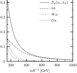
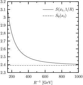
Figure 2: (a) Contribution $S_{n}$ of the $n^{\rm th}$ KK mode to $S(x_{t},1/R)$. The contributions with $a^{\pm}$ dominate, those with only $G^{\pm}$ and $W^{\pm}$ are negligible and not shown. (b) The functions $S(x_{t},1/R)$ and $S_{0}(x_{t})$.

Proceeding as in the SM, we can calculate the mass differences $\Delta M_{q}$ by means of

$$\Delta M_{q}=\frac{G_{\rm F}^{2}}{6\pi^{2}}\eta_{B}m_{B_{q}}(\hat{B}_{B_{q}}F_{B_{q}}^{2})M_{W}^{2}S(x_{t},1/R)|V_{tq}|^{2},$$ (3.11)

where $F_{B_{q}}$ is the $B_{q}$-meson decay constant and $\hat{B}_{q}$ the renormalization group invariant parameter related to the hadronic matrix element of the operator $Q(\Delta B=2)$, see [25] for details. This implies two useful formulae

$$\Delta M_{d}=0.50/{\rm ps}\cdot\left[\frac{\sqrt{\hat{B}_{B_{d}}}F_{B_{d}}}{230\,{\rm MeV}}\right]^{2}\left[\frac{|V_{td}|}{7.8\cdot 10^{-3}}\right]^{2}\left[\frac{\eta_{B}}{0.55}\right]\left[\frac{S(x_{t},1/R)}{2.34}\right]$$ (3.12)

and

$$\Delta M_{s}=18.4/{\rm ps}\cdot\left[\frac{\sqrt{\hat{B}_{B_{s}}}F_{B_{s}}}{270\,{\rm MeV}}\right]^{2}\left[\frac{|V_{ts}|}{0.040}\right]^{2}\left[\frac{\eta_{B}}{0.55}\right]\left[\frac{S(x_{t},1/R)}{2.34}\right]~{}.$$ (3.13)

The implications of these results for $|V_{td}|$, $\Delta M_{s}$ and the unitarity triangle will be discussed below.

Finally, a few comments regarding the QCD factor $\eta_{B}$ are in order. This factor as given in (3.3) has been calculated within the SM including NLO QCD corrections that are mandatory for the proper matching of the Wilson coefficient of the operator $Q(\Delta B=2)$ with its hadronic matrix element represented by the parameter $\hat{B}_{B_{s,d}}$ and calculated by means of non-perturbative methods. As the top quark and the KK modes are integrated out at a single scale $\mu_{t}={\cal O}(m_{\rm t},1/R)$, the contributions to $\eta_{B}$ from scales lower than $\mu_{t}$ are the same for the SM and the ACD model. They simply describe the finite renormalization of $Q(\Delta B=2)$ from scales ${\cal O}(\mu_{t})$ down to the scales ${\cal O}(m_{b})$. The difference between QCD corrections to the SM contributions and to the KK contributions arises only in the full theory at scales $\mu_{t}={\cal O}(m_{\rm t},1/R)$ as the unknown QCD corrections to the box diagrams in fig. 1 can in principle differ from the known QCD corrections to the SM box diagrams [23, 24] that have been included in $\eta_{B}$. As the QCD coupling constant $\alpha_{s}(\mu_{t})$ is small and the QCD corrections to the SM box diagrams of order of a few percent, we do not expect that the difference between the QCD corrections to the diagrams in fig. 1 and to the SM box diagrams is relevant, in particular in view of the fact that the KK contributions amount to at most $17\%$ of the full result.

For $\mu\gg\mu_{t}$, $\alpha_{s}(\mu)$ in the ACD model becomes larger [26] and the QCD corrections to KK modes with $n\gg 1$ could in principle be substantial. However, as seen in fig. 2, these heavy modes give only a tiny contribution to $S(x_{t},1/R)$ and can be safely neglected.

3.2 $\varepsilon_{K}$

The effective Hamiltonian for $\Delta S=2$ transitions is given in the ACD model as follows

$${\cal H}^{\Delta S=2}_{\rm eff} = \frac{G^{2}_{\rm F}}{16\pi^{2}}M^{2}_{W}\left[\lambda^{2}_{c}\eta_{1}S_{0}(x_{c})+\lambda^{2}_{t}\eta_{2}S(x_{t},1/R)+2\lambda_{c}\lambda_{t}\eta_{3}S_{0}(x_{c},x_{t})\right]\times$$ (3.14)

$$\times\left[\alpha_{s}^{(3)}(\mu)\right]^{-2/9}\left[1+\frac{\alpha_{s}^{(3)}(\mu)}{4\pi}J_{3}\right]Q(\Delta S=2)+h.c.$$

where $\lambda_{i}=V_{is}^{*}V_{id}$, $\alpha_{s}^{(3)}$ is the strong coupling constant in an effective three flavour theory and $J_{3}=1.895$ in the NDR scheme [23]. In (3.14), the relevant operator

$$Q(\Delta S=2)=(\bar{s}d)_{V-A}(\bar{s}d)_{V-A},$$ (3.15)

is multiplied by the corresponding Wilson coefficient function. This function is decomposed into a charm-, a top- and a mixed charm-top contribution. The SM function $S_{0}(x_{c},x_{t})$ is defined by

$$S_{0}(x_{c},x_{t})=F(x_{c},x_{t})+F(x_{u},x_{u})-F(x_{c},x_{u})-F(x_{t},x_{u}),$$ (3.16)

where $F(x_{i},x_{j})$ is the true function corresponding to the box diagrams with $(i,j)$ exchanges. One has

$$S_{0}(x_{c},x_{t})=x_{c}\left[\ln\frac{x_{t}}{x_{c}}-\frac{3x_{t}}{4(1-x_{t})}-\frac{3x^{2}_{t}\ln x_{t}}{4(1-x_{t})^{2}}\right]\,,$$ (3.17)

where we keep only linear terms in $x_{c}\ll 1$, but of course all orders in $x_{t}$.

In view of the comments made after (3.8) and the structure of (3.16), the impact of the KK modes on the charm- and mixed charm-top contributions is totally negligible and we take into account these modes only in the top contribution that is described by the same function $S(x_{t},1/R)$ as in the case of $\Delta M_{q}$. This also means that the $K_{L}-K_{S}$ mass difference, $\Delta M_{K}$, being dominated by internal charm contributions in (3.14) is practically uneffected by the KK modes.

Short distance QCD effects are described through the correction factors $\eta_{1}$, $\eta_{2}$, $\eta_{3}$ and the explicitly $\alpha_{s}$-dependent terms in (3.14). The NLO values of $\eta_{i}$ are given as follows [27, 23, 28]:

$$\eta_{1}=1.45\pm 0.38,\qquad\eta_{2}=0.57\pm 0.01,\qquad\eta_{3}=0.47\pm 0.04~{}.$$ (3.18)

The standard procedure allows now to calculate the CP-violating parameter $\varepsilon_{K}$ [25]

$$\varepsilon_{K}=C_{\varepsilon}\hat{B}_{K}{\rm Im}\lambda_{t}\left\{{\rm Re}\lambda_{c}\left[\eta_{1}S_{0}(x_{c})-\eta_{3}S_{0}(x_{c},x_{t})\right]-{\rm Re}\lambda_{t}\eta_{2}S(x_{t},1/R)\right\}\exp(i\pi/4)\,,$$ (3.19)

where $C_{\varepsilon}=3.837\cdot 10^{4}$ is a numerical constant. $\hat{B}_{K}$ is the renormalization group invariant parameter related to the hadronic matrix element of the operator $Q(\Delta S=2)$, see [25] for details.

3.3 Unitarity Triangle in the ACD Model

What is the impact of the KK contributions to the function $S$ on the elements of the CKM matrix and in particular on the shape of the unitarity triangle? In order to answer this question let us recall a few aspects of the unitarity triangle (UT) shown in fig. 3 and of the Wolfenstein parametrization [29] as generalized to higher orders in $\lambda$ in [30]. The apex of the unitarity triangle is given by [30]

$$\bar{\varrho}=\varrho(1-\frac{\lambda^{2}}{2}),\qquad\bar{\eta}=\eta(1-\frac{\lambda^{2}}{2}).$$ (3.20)

Here $\lambda$, A, $\varrho$ and $\eta$ are the Wolfenstein parameters [29]. Moreover, one has

$$V_{us}=\lambda+{\cal O}(\lambda^{7}),\qquad V_{ub}=A\lambda^{3}(\varrho-i\eta),\qquad V_{cb}=A\lambda^{2}+{\cal O}(\lambda^{8}),$$ (3.21)

$$V_{ts}=-A\lambda^{2}+\frac{1}{2}A\lambda^{4}[1-2(\varrho+i\eta)],\qquad V_{td}=A\lambda^{3}(1-\bar{\varrho}-i\bar{\eta})~{}.$$ (3.22)

Figure 3: Unitarity Triangle.

The lengths $R_{b}$ and $R_{t}$ are given by

$$R_{b}\equiv\frac{|V_{ud}V^{*}_{ub}|}{|V_{cd}V^{*}_{cb}|}=\sqrt{\bar{\varrho}^{2}+\bar{\eta}^{2}}=(1-\frac{\lambda^{2}}{2})\frac{1}{\lambda}\left|\frac{V_{ub}}{V_{cb}}\right|,$$ (3.23)

$$R_{t}\equiv\frac{|V_{td}V^{*}_{tb}|}{|V_{cd}V^{*}_{cb}|}=\sqrt{(1-\bar{\varrho})^{2}+\bar{\eta}^{2}}=\frac{1}{\lambda}\left|\frac{V_{td}}{V_{cb}}\right|$$ (3.24)

and the angles $\beta$ and $\gamma$ of the UT are related directly to the complex phases of the CKM elements $V_{td}$ and $V_{ub}$, respectively, through

$$V_{td}=|V_{td}|e^{-i\beta},\quad V_{ub}=|V_{ub}|e^{-i\gamma}.$$ (3.25)

The five constraints on the UT that we have at our disposal at present are:

• The $R_{b}$ Constraint: As seen in (3.23), the length of the side AC is determined from $|V_{ub}/V_{cb}|$.

• $\varepsilon_{K}$–Hyperbola (Indirect CP Violation in $K_{L}\to\pi\pi$) obtained from (3.19) and the experimental value for $\varepsilon_{K}$ ($\lambda=0.221$):

  $$\bar{\eta}\left[(1-\bar{\varrho})A^{2}\eta_{2}S(x_{t},1/R)+P_{c}(\varepsilon)\right]A^{2}\hat{B}_{K}=0.214~{},$$ (3.26)

  where $P_{c}(\varepsilon)=0.28\pm 0.05$ [27, 28] represents the charm contribution that is not affected by the KK contributions.

• $B^{0}_{d}-\bar{B}^{0}_{d}$–Mixing Constraint ($\Delta M_{d}$):

  $$R_{t}=\frac{1}{\lambda}\frac{|V_{td}|}{|V_{cb}|}=0.86\cdot\left[\frac{|V_{td}|}{7.8\cdot 10^{-3}}\right]\left[\frac{0.041}{|V_{cb}|}\right]$$ (3.27)

  with

  $$|V_{td}|=7.8\cdot 10^{-3}\left[\frac{230\,{\rm MeV}}{\sqrt{\hat{B}_{B_{d}}}F_{B_{d}}}\right]\sqrt{\frac{\Delta M_{d}}{0.50/{\rm ps}}}\sqrt{\frac{0.55}{\eta_{B}}}\sqrt{\frac{2.34}{S(x_{t},1/R)}}$$ (3.28)

  where $\Delta M_{d}=(0.503\pm 0.006)/{\rm ps}$ [31].

• $B^{0}_{s}-\bar{B}^{0}_{s}$–Mixing Constraint ($\Delta M_{d}/\Delta M_{s}$):

  $$R_{t}=0.87~{}\sqrt{\frac{\Delta M_{d}}{0.50/{\rm ps}}}\sqrt{\frac{18.4/{\rm ps}}{\Delta M_{s}}}\left[\frac{\xi}{1.18}\right],\qquad\xi=\frac{\sqrt{\hat{B}_{s}}F_{B_{s}}}{\sqrt{\hat{B}_{d}}F_{B_{d}}}$$ (3.29)

  where $\Delta M_{s}>14.4/{\rm ps}$ at $95\%$ C.L. [31].

• The direct measurement of $\sin 2\beta$ through the CP asymmetry $a(\psi K_{S})$ in $B_{d}\to\psi K_{S}$ that is not affected by the KK contributions.

The main uncertainties in this analysis originate in the theoretical uncertainties in the non-perturbative parameters $\hat{B}_{K}$ and $\sqrt{\hat{B}_{d}}F_{B_{d}}$ and to a lesser extent in $\xi$ [32]:

$$\hat{B}_{K}=0.86\pm 0.15,\qquad\sqrt{\hat{B}_{d}}F_{B_{d}}=(235^{+33}_{-41})~{}{\rm MeV},\qquad\xi=1.18^{+0.13}_{-0.04}.$$ (3.30)

Also the uncertainties in $|V_{ub}/V_{cb}|$ and $\sqrt{\hat{B}_{s}}F_{B_{s}}=(276\pm 38)~{}{\rm MeV}$ are substantial. The QCD sum rules results for the parameters in question are similar and can be found in [33].

With these formulae at hand let us enumerate a few general properties of the values of the CKM elements within the ACD model. These are:

• $|V_{us}|$, $|V_{cb}|$ and $|V_{ub}|$ are usually determined from tree level decays. As in the ACD model there are no KK contributions at the tree level, the absolute values of these three CKM elements are to an excellent approximation the same as in the SM model. From the point of view of the unitarity triangle (UT), this means that the lengths of its two sides, AC and CB are common to the SM model and the ACD model. In our numerical analysis we will use, as in [34],

  $$|V_{us}|=\lambda=0.221\pm 0.002\,\quad\quad|V_{cb}|=(40.6\pm 0.8)\cdot 10^{-3},$$ (3.31)

  $$\frac{|V_{ub}|}{|V_{cb}|}=0.089\pm 0.008,\quad\quad|V_{ub}|=(3.63\pm 0.32)\cdot 10^{-3}.$$ (3.32)

• The angle $\beta$ of the UT has been determined recently by the BaBar [35] and Belle [36] collaborations from the CP asymmetry $a_{\psi K_{S}}$ in $B\to\psi K_{S}$ with a high accuracy giving the world grand average [37]

  $$(\sin 2\beta)_{\psi K_{S}}=0.734\pm 0.054~{}.$$ (3.33)

  As there are no new complex phases in the ACD model beyond the KM phase, the angle $\beta$ as extracted by means of $a_{\psi K_{S}}$ is common to both models in question.

• A similar comment applies to $|V_{td}|$ or equivalently the length $R_{t}$ of the side AB in fig. 3, when $R_{t}$ is extracted from the ratio $\Delta M_{d}/\Delta M_{s}$ that is independent of $S(x_{t},1/R)$ as seen in (3.29).

Thus when $|V_{ub}/V_{cb}|$, $\sin 2\beta$ from $a_{\psi K_{S}}$ and $\Delta M_{d}/\Delta M_{s}$ are used to construct the UT, there is no difference between the SM and the ACD model as all explicit dependence on $1/R$ cancels out. This universal UT (UUT) [14] that is valid for all MVF models, as defined in [14], has recently been determined [34, 38].

Now, even though there exists a UUT common to the SM and the ACD model, in view of the fact that $S(x_{t},1/R)\not=S_{0}(x_{t})$, only one of these two models, if any, will have $\varepsilon_{K}$, $\Delta M_{d}$ and $\Delta M_{s}$ that agree with the experimental data. Let us consider $\Delta M_{s}$ first. As seen in (3.22) $|V_{ts}|$ is very close to $|V_{cb}|$ because of CKM unitarity. Therefore it is common with an excellent accuracy to both models and consequently

$$\frac{(\Delta M_{s})_{\rm ACD}}{(\Delta M_{s})_{\rm SM}}=\frac{S(x_{t},1/R)}{S_{0}(x_{t})}>1.$$ (3.34)

However, this ratio is at most $1.17$ and the distinction between these two models will only be possible provided $\hat{B}_{B_{s}}F_{B_{s}}^{2}$ can be calculated to better than $10\%$ accuracy. A very difficult task.

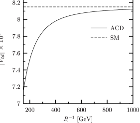
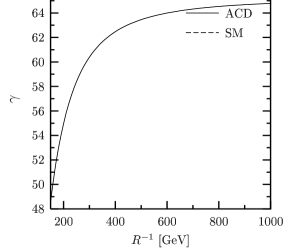
Figure 4: Results for various CKM parameters in the ACD model and in the SM: (a) $\left|V_{td}\right|$ (b) $\gamma$ (c) $\bar{\eta}$ (d) $\bar{\rho}$.

The fact that $S(x_{t},1/R)>S_{0}(x_{t})$ implies also that with the experimentally known values of $\varepsilon_{K}$ and $\Delta M_{d}$, one has

$$|V_{td}|_{\rm ACD}<|V_{td}|_{\rm SM},\qquad\gamma_{\rm ACD}<\gamma_{\rm SM}$$ (3.35)

as can easily be inferred from (3.26) and (3.28). In particular (3.28) implies

$$\frac{|V_{td}|_{\rm ACD}}{|V_{td}|_{\rm SM}}=\sqrt{\frac{S_{0}(x_{t})}{S(x_{t},1/R)}}.$$ (3.36)

Thus $|V_{td}|_{\rm ACD}$ can be smaller than $|V_{td}|_{\rm SM}$ by at most $8\%$. In order to determine such a difference, more accurate information on the unitarity triangle and the non-perturbative parameters entering $\varepsilon_{K}$ and $\Delta M_{d,s}$ is necessary. Similarly $\gamma_{\rm ACD}$ can be smaller than $\gamma_{\rm SM}$ by at most $10$ degrees.

We illustrate these properties in fig. 4, where we show the $1/R$ dependence of $|V_{td}|$, $\gamma$, $\bar{\varrho}$ and $\bar{\eta}$. In obtaining these results we used the following procedure. First using the central value $|V_{td}|_{\rm SM}=0.00815$ from the SM fit of [34] and $m_{t}=167\,{\rm GeV}$ we determined $|V_{td}|_{\rm ACD}$ by means of (3.36). The result is shown in fig. 4. Using next the central values in (3.31) and (3.32) and the $1/R$ dependence of $(R_{t})_{\rm ACD}=|V_{td}|_{\rm ACD}/(\lambda|V_{cb}|)$, we determined $\gamma$, $\bar{\varrho}$ and $\bar{\eta}$ as functions of $1/R$. We show in fig. 5 the unitarity triangles corresponding to the ACD model with $1/R=200\,{\rm GeV}$ and the SM model.

Figure 5: Unitarity Triangle in the ACD model for $1/R=200\,{\rm GeV}$ and in the SM.

In summary, the CKM elements in the ACD model extracted from $\Delta F=2$ transitions and the CP asymmetry $a_{\psi K_{S}}$ are not expected to differ substantially from the corresponding values found within the SM. This is very fortunate as the most recent fits of the UT [34, 37, 39, 40, 41, 42] based on the SM expressions for $\Delta F=2$ transitions agree very well with the direct measurement of the angle $\beta$ by means of $a_{\psi K_{S}}$. With improved data on $a_{\psi K_{S}}$ and in particular $\Delta M_{s}$ and improved values for $\hat{B}_{K}$ and $\hat{B}_{B_{q}}F_{B_{q}}^{2}$, a constraint on the compactification radius $R$ from $\Delta F=2$ processes is in principle possible. However, for the time being even the lowest value $1/R=200~{}\,{\rm GeV}$ considered by us is consistent with the present fits of the UT. Setting $1/R=200~{}\,{\rm GeV}$ and repeating the analysis of [34], that uses the bayesian method [39], one finds [43] the values for $(\bar{\varrho},\bar{\eta})$, $\sin 2\alpha$, $\gamma$, $\Delta M_{s}$ and $|V_{td}|$ in the second column of table 1. For a comparison we give the corresponding ranges in the SM. To this end all input parameters of [34] have been used.

Comparing the two columns in table 1, we observe all the patterns shown in fig. 4. However, due to substantial uncertainties in the input parameters, the effects of the KK modes are partly washed out. In particular, the suppressions of $|V_{td}|$ and $\bar{\eta}$ amount to $4-5\%$ rather than ${\cal O}(10\%)$ that we found in fig. 4. This is easy to understand. With no uncertainty in $\sqrt{\hat{B}_{B_{d}}}F_{B_{d}}$, the value of $|V_{td}|$ is strongly correlated with $S(x_{t},1/R)$ by means of (3.12) as $\Delta M_{d}$ is known very well experimentally. Once the uncertainties in $\sqrt{\hat{B}_{B_{d}}}F_{B_{d}}$ are taken into account, the enhancement of the function $S$ in the ACD model can be compensated by the decrease of both $|V_{td}|$ and $\sqrt{\hat{B}_{B_{d}}}F_{B_{d}}$, implying a smaller suppression of $|V_{td}|$ than found in fig. 4. Similar comments can be made in connection with other quantities in table 1.

Clearly, low energy non-perturbative parameters as $\sqrt{\hat{B}_{B_{d}}}F_{B_{d}}$, $\hat{B}_{K}$ and $\xi$ do not depend on the compactification scale. On the other hand they are subject to uncertainties and it is not surprising that the fit of the unitarity triangle within the ACD model prefers lower values of $\sqrt{\hat{B}_{B_{d}}}F_{B_{d}}$ and $\hat{B}_{K}$ than in the SM. The true effects of the KK modes can then only be clearly seen as in fig. 4 when the input parameters have no uncertainties. This exercise shows very clearly the importance of the reduction of the theoretical uncertainties in connection with the search for new physics.

Strategy	ACD ($1/R=200\,{\rm GeV}$)	SM
$\bar{\eta}$	0.342 $\pm$ 0.027	0.357 $\pm$ 0.027
	$(0.288-0.398)$	$(0.305-0.411)$
$\bar{\rho}$	0.197 $\pm$ 0.047	0.173 $\pm$ 0.046
	$(0.102-0.296)$	$(0.076-0.260)$
$\sin 2\alpha$	$-0.23\pm 0.25$	$-0.09\pm 0.25$
	$(-0.70-0.27)$	$(-0.54-0.40)$
$\gamma$	59.5 $\pm$ 7.0	63.5 $\pm$ 7.0
(degrees)	$(45.3-74.8)$	$(51.0-79.0)$
$\Delta M_{s}$	18.6${}^{+1.9}_{-1.5}$	18.0${}^{+1.7}_{-1.5}$
($ps^{-1}$)	$(15.7-26.2)$	$(15.4-21.7)$
$|V_{td}|~{}(10^{-3})$	7.80 $\pm$ 0.42	8.15 $\pm$ 0.41
	$(6.96-8.69)$	$(7.34-8.97)$

Table 1: Values and errors for different quantities in the ACD model with $1/R=200\,{\rm GeV}$ [43] and in the SM from [34]. The 95$\%$ probability regions are given in brackets.

This discussion makes it clear that it is impossible to claim, as done in [18], that the reduction of the error on the parameter $\sqrt{\hat{B}_{B_{d}}}F_{B_{d}}$ by a factor of three will necessarily increase the lowest allowed value of the compactification scale $1/R$. The lower bound on $1/R$ from $\Delta M_{d}$ depends necessarily on the actual value of $\sqrt{\hat{B}_{B_{d}}}F_{B_{d}}$. With decreasing $\sqrt{\hat{B}_{B_{d}}}F_{B_{d}}$ the lower bound on $1/R$ becomes weaker. One can easily check that decreasing the central value for $\sqrt{\hat{B}_{B_{d}}}F_{B_{d}}$ to $200\,{\rm MeV}$, still within the present uncertainties, no significant lower bound on $1/R$ can be obtained even if the error on $\sqrt{\hat{B}_{B_{d}}}F_{B_{d}}$ is decreased by a factor of three.

Figure 6: Correlation between $1/R$ and $\sqrt{\hat{B}_{B_{d}}}F_{B_{d}}$ for different values of $|V_{td}|$.

In order to illustrate this point we show in fig. 6 the correlation between $1/R$ and $\sqrt{\hat{B}_{B_{d}}}F_{B_{d}}$ for different values of $|V_{td}|$ and $m_{t}=167\,{\rm GeV}$. To this end we have used (3.12) with $\Delta M_{d}=0.503/ps$. Clearly on the basis of $\Delta M_{d}$ alone it is impossible to say anything about $1/R$. However, even if $|V_{td}|$ is determined through $\Delta M_{d}/\Delta M_{s}$, the values of $1/R$ depend sensitively on $\sqrt{\hat{B}_{B_{d}}}F_{B_{d}}$ with the maximal and minimal values of $\sqrt{\hat{B}_{B_{d}}}F_{B_{d}}$ corresponding to maximal and minimal values of $1/R$, respectively. Thus a significantly improved lower bound on $\sqrt{\hat{B}_{B_{d}}}F_{B_{d}}$ could in principle provide an improved lower bound on $1/R$. However, if future lattice calculations will find values for $\sqrt{\hat{B}_{B_{d}}}F_{B_{d}}$ that are smaller than the present central value, $1/R$ could be forced to be low in order for the ACD model to fit the value of $\Delta M_{d}$.

4 Rare K and B Decays

4.1 Preliminaries

We will now move to discuss the semileptonic rare FCNC transitions $K^{+}\rightarrow\pi^{+}\nu\bar{\nu}$, $K_{\rm L}\to\pi^{0}\nu\bar{\nu}$, $K_{L}\to\mu\bar{\mu}$, $B\to X_{s,d}\nu\bar{\nu}$ and $B_{s,d}\to\mu\bar{\mu}$. Within the SM and the ACD model these decays are loop-induced semileptonic FCNC processes governed by $Z^{0}$-penguin and box diagrams and described by two functions $X(x_{t},1/R)$ and $Y(x_{t},1/R)$ for the decays with $\nu\bar{\nu}$ and $\mu\bar{\mu}$ in the final state, respectively.

A particular and very important virtue of these decays (with the exception of $K_{L}\to\mu\bar{\mu}$) is their clean theoretical character [25] that allows to probe high energy scales of the theory and in particular to measure $V_{td}$ and ${\rm Im}\lambda_{t}={\rm Im}V^{*}_{ts}V_{td}$ from $K^{+}\to\pi^{+}\nu\bar{\nu}$ and $K_{\rm L}\to\pi^{0}\nu\bar{\nu}$ respectively. Moreover, the combination of these two decays offers one of the cleanest measurements of $\sin 2\beta$ [44], see [44, 45] for more details.

4.2 Effective Hamiltonians for $K\to\pi\nu\bar{\nu}$ and $B\to X_{s}\nu\bar{\nu}$

The effective Hamiltonian for $K^{+}\rightarrow\pi^{+}\nu\bar{\nu}$ is given in the ACD model as follows

$${\cal H}_{\rm eff}={G_{\rm F}\over{\sqrt{2}}}{\alpha\over 2\pi\sin^{2}\theta_{w}}\sum_{l=e,\mu,\tau}\left(V^{\ast}_{cs}V_{cd}X^{l}_{\rm NL}+V^{\ast}_{ts}V_{td}\eta_{X}X(x_{t},1/R)\right)(\bar{s}d)_{V-A}(\bar{\nu}_{l}\nu_{l})_{V-A}\,.$$ (4.1)

The index $l$=$e$, $\mu$, $\tau$ denotes the lepton flavour. The dependence on the charged lepton mass resulting from the box diagram is negligible for the top contribution. In the charm sector this is the case only for the electron and the muon but not for the $\tau$-lepton. In what follows we will set the QCD factor $\eta_{X}$ [46, 47, 48] to unity as for $m_{\rm t}\equiv\overline{m}_{t}(m_{\rm t})$ it equals $0.994$.

The function $X(x_{t},1/R)$ relevant for the top part is given by

$$X(x_{t},1/R)=C(x_{t},1/R)+B^{\nu\bar{\nu}}(x_{t},1/R).$$ (4.2)

Here

$$C(x_{t},1/R)=C_{0}(x_{t})+\sum_{n=1}^{\infty}C_{n}(x_{t},x_{n})$$ (4.3)

results from $Z^{0}$-penguin diagrams with the SM contribution $C_{0}(x_{t})$ given by

$$C_{0}(x_{t})={x_{t}\over 8}\left[{{x_{t}-6}\over{x_{t}-1}}+{{3x_{t}+2}\over{(x_{t}-1)^{2}}}\;\ln x_{t}\right]~{}.$$ (4.4)

The sum in (4.3) represents the KK contributions that are calculated from the Feynman diagrams in fig. 7 as discussed below. Next

$$B^{\nu\bar{\nu}}(x_{t},1/R)=-4B_{0}(x_{t})+\sum_{n=1}^{\infty}B^{\nu\bar{\nu}}_{n}(x_{t},x_{n})$$ (4.5)

results from box diagrams with the SM contribution given by the first term and

$$B_{0}(x_{t})={1\over 4}\left[{x_{t}\over{1-x_{t}}}+{{x_{t}\ln x_{t}}\over{(x_{t}-1)^{2}}}\right].$$ (4.6)

The sum in (4.5) represents the KK contributions that are calculated from the Feynman diagrams in fig. 9 as discussed below.

The expression corresponding to $X(x_{t},1/R)$ in the charm sector is the function $X^{l}_{\rm NL}$. It results from the NLO calculation [49] and is given explicitly in [48] where further details can be found. As in the case of the charm contributions in the $\Delta S=2$ Hamiltonian, here the KK contributions are also negligible. The numerical values for $X^{l}_{\rm NL}$ for $\mu=m_{\rm c}$ and several values of $\Lambda_{\overline{\rm MS}}^{(4)}$ and $m_{\rm c}(m_{\rm c})$ can be found in [48]. For our purposes we need only ($\lambda=0.221$)

$$P_{0}(X)=\frac{1}{\lambda^{4}}\left[\frac{2}{3}X^{e}_{\rm NL}+\frac{1}{3}X^{\tau}_{\rm NL}\right]=0.41\pm 0.06~{},$$ (4.7)

where the error results from the variation of $\Lambda_{\overline{\rm MS}}^{(4)}$ and $m_{\rm c}(m_{\rm c})$.

In the case of $K_{\rm L}\rightarrow\pi^{0}\nu\bar{\nu}$ that is governed by CP-violating contributions only the top contribution in (4.1) matters. Similarly the effective Hamiltonians for $B\to X_{s,d}\nu\bar{\nu}$ are obtained from (4.1) by neglecting the charm contribution and changing appropriately the CKM factor and quark flavours. In all these decays the KK modes contribute universally only through the function $X(x_{t},1/R)$.

4.3 Effective Hamiltonians for $B_{s,d}\to\mu\bar{\mu}$ and $K_{L}\to\mu\bar{\mu}$

The effective Hamiltonian for $B_{s}\to l^{+}l^{-}$ in the ACD model is given as follows:

$${\cal H}_{\rm eff}=-{G_{\rm F}\over\sqrt{2}}{\alpha\over 2\pi\sin^{2}\theta_{w}}V^{\ast}_{tb}V_{ts}\eta_{Y}Y(x_{t},1/R)(\bar{b}s)_{V-A}(\bar{l}l)_{V-A}+h.c.$$ (4.8)

with $s$ replaced by $d$ in the case of $B_{d}\to l^{+}l^{-}$. The charm contributions are fully negligible here. In what follows we will set the QCD factor $\eta_{Y}$ [46, 47, 48] to unity as for $m_{\rm t}\equiv\overline{m}_{t}(m_{\rm t})$ it equals $1.012$.

The function $Y(x_{t},1/R)$ is given in the ACD model by

$$Y(x_{t},1/R)=C(x_{t},1/R)+B^{\mu\bar{\mu}}(x_{t},1/R),$$ (4.9)

with $C(x_{t},1/R)$ given in (4.3) and

$$B^{\mu\bar{\mu}}(x_{t},1/R)=-B_{0}(x_{t})+\sum_{n=1}^{\infty}B^{\mu\bar{\mu}}_{n}(x_{t},x_{n})$$ (4.10)

with the first term representing the SM contribution. The second term results from the box diagrams in fig. 9.

The effective Hamiltonian for the short distance contribution to $K_{L}\to\mu\bar{\mu}$ is given by (4.8) with the appropriate change of the CKM factors and quark flavours and a small SM charm contribution $Y_{\rm NL}$ [48] in analogy to $X^{l}_{\rm NL}$ in (4.1). The relevant branching ratio will be given below.

4.4 $Z^{0}$-Penguin Diagrams

The function $C_{n}(x_{t},x_{n})$ can be found by calculating the vertex diagrams in fig. 7 and adding an electroweak counter term as discussed in detail in [50]. The latter is found by calculating the self-energy diagrams of fig. 12 that describe flavour non-diagonal propagation of quark fields and subsequently rotating the quark fields appropriately so that this flavour non-diagonal propagation does not take place in the new fields.

Figure 7: Penguin diagrams contributing to $C_{n}(x_{t},x_{n})$. The analytical expressions are listed in appendix C. $(8)$ includes the additional diagram with $W^{\pm}$ and $(a^{\pm},G^{\pm})$ interchanged.

In the ’t Hooft-Feynman gauge for the $W_{(n)}^{\pm}$ and $G_{(n)}^{\pm}$ propagators, the contribution of the diagrams in fig. 7 to the flavour-changing vertex $\Gamma_{Z}^{\mu}$ including the electroweak counterterm is given by

$$\Delta\Gamma_{Z}^{\mu}=i\frac{g_{2}^{3}}{16\pi^{2}\cos\theta_{w}}V_{ts}^{*}V_{td}C_{n}(x_{t},x_{n})\bar{s}\gamma_{\mu}(1-\gamma_{5})d.$$ (4.11)

We neglect the external momenta in fig. 7 and the masses of external quarks. The function $C_{n}(x_{t},x_{n})$ is defined through

$$C_{n}(x_{t},x_{n})=F(x_{t(n)})-F(x_{u(n)})$$ (4.12)

with the functions $F(x_{t(n)})$ and $F(x_{u(n)})$ representing the contributions of the $\mathcal{Q}_{t(n)}$, $\mathcal{U}_{t(n)}$ and $\mathcal{Q}_{u(n)}$, $\mathcal{U}_{u(n)}$ modes, respectively,

$$F(x_{t(n)})=\sum_{i=1}^{8}F_{i}(x_{t(n)})+\left(\frac{1}{2}-\frac{1}{3}s_{w}^{2}\right)\sum_{i=1}^{2}\Delta S_{i}(x_{t(n)}).$$ (4.13)

Here $s_{w}\equiv\sin\theta_{w}$, $F_{i}$ stand for the contributions of diagrams in fig. 7 and $\Delta S_{i}$ denote the electroweak counter terms.

The explicit contributions of various sets of diagrams to these functions are given in appendix C. Adding up these contributions we find

$$C_{n}(x_{t},x_{n})=\frac{x_{t}}{8(x_{t}-1)^{2}}\left[x_{t}^{2}-8x_{t}+7+(3+3x_{t}+7x_{n}-x_{t}x_{n})\ln\frac{x_{t}+x_{n}}{1+x_{n}}\right].$$ (4.14)

In fig. 8, we show $C_{n}(x_{t},x_{n})$ as a function of $n/R$. In this case the convergence of the sum of the KK modes is significantly improved by the GIM mechanism so that only a few first terms in the sum in (4.3) are relevant. We will return to this at the end of this section. We observe that in contrast to the function $S$ of section 3 the diagrams involving only $W^{\pm}_{(n)}$ play the dominant role among the KK contributions.

In fig. 8 we plot $C(x_{t},1/R)$ versus $1/R$. For $1/R=200\,{\rm GeV}$ we observe a $38\%$ enhancement of the function $C$ with respect to its SM value given by $C_{0}(x_{t})$. For $1/R=250\,{\rm GeV}$ this enhancement decreases to $26\%$ and it is $11\%$ for $1/R=400\,{\rm GeV}$. The significant enhancement of $C$ is the origin of the enhancements of the branching ratios discussed below.

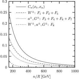
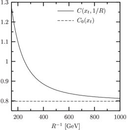
Figure 8: (a) Contribution $C_{n}$ of the $n^{\rm th}$ KK mode to $C(x_{t},1/R)$. The functions $F_{i}$ correspond to the diagrams given in fig. 7. (b) The functions $C(x_{t},1/R)$ and $C_{0}(x_{t})$.

4.5 $Z^{0}b\bar{b}$ Vertex in the large $m_{t}$ limit

The result in (4.14) can also be used to find the dominant KK contribution to the $Z^{0}b\bar{b}$ vertex in the large $m_{t}$ limit. As discussed already in [50], in general the calculation of a low energy effective flavour violating $Z^{0}d\bar{s}$ vertex cannot be directly compared with the full calculation of the $Z^{0}b\bar{b}$ vertex. However, as pointed out there in the special limiting case $m_{t}\gg M_{W}$ the two approaches, the direct evaluation of on-shell diagrams and the operator product expansion considered by us, are equivalent. The reason for this is that in the limit $m_{t}\gg M_{W}$ with $1/R\geq m_{t}$ all the other mass scales as $m_{b}$ and external momenta of $b$-quarks become negligible compared with $m_{t}$ and $1/R$. Consequently with the definition

$$\Gamma^{\mu}_{Zb\bar{b}}=i\frac{g_{2}}{\cos\theta_{w}}\bar{b}\gamma^{\mu}(g_{L}P_{L}+g_{R}P_{R})b$$ (4.15)

the one-loop contributions to the coupling $g_{L}$ can be found in the large $m_{t}$ limit by using the relation [50]

$$\delta g_{L}=\frac{G_{F}}{\sqrt{2}}\frac{M_{W}^{2}}{\pi^{2}}C(x_{t},1/R).$$ (4.16)

In the case of the SM contributions this relation has been already analyzed in detail in [50] including $\alpha_{s}$ to the one-loop $Z^{0}b\bar{b}$ vertex. For the KK contribution we find from (4.14)

$$\Delta C\!=\!\sum_{n=1}^{\infty}C_{n}(x_{t},x_{n})\!=\!\left(\frac{m_{t}^{4}{\pi}^{2}}{96\,m_{W}^{2}}+\frac{m_{t}^{2}{\pi}^{2}}{96}\right)R^{2}+\left(\frac{m_{t}^{4}{\pi}^{4}}{4320}-\frac{m_{t}^{6}{\pi}^{4}}{2160\,m_{W}^{2}}-\frac{m_{t}^{2}m_{W}^{2}{\pi}^{4}}{864}\right)R^{4}+\ldots$$

with the dominant contribution represented by the first term, see appendix D for the derivation. Retaining only this term and using (4.16) we find

$$\delta g_{L}^{KK}=\frac{G_{F}}{\sqrt{2}}m_{t}^{4}\frac{R^{2}}{96}$$ (4.18)

that agrees with a recent direct calculation of the KK contributiond to the $Zb\bar{b}$ vertex in [51], see their formula (3.6). Interestingly, while the corrections to the asymptotic result (4.18) relevant for the $Zb\bar{b}$ vertex have been found in [51] to be substantial, the result

$$\Delta C=\frac{m_{t}^{4}\pi^{2}}{96M_{W}^{2}}R^{2}$$ (4.19)

give a good approximation to the full KK contribution to the function $C(x_{t},1/R)$ even for $m_{t}\approx 167\,{\rm GeV}$.

4.6 Box Diagram Contributions

The functions $B^{\nu\bar{\nu}}_{n}(x_{t},x_{n})$ and $B^{\mu\bar{\mu}}_{n}(x_{t},x_{n})$ can be found by appropriate rescaling of the box diagrams contributing to $\Delta F=2$ transitions that we considered in section 3. It turns out that the box contributions of the KK modes are tiny. For instance for $1/R=200\,{\rm GeV}$ and $m_{\rm t}=167\,{\rm GeV}$ we find $B^{\nu\bar{\nu}}_{1}(x_{t},x_{1})=0.0098$ and $B^{\mu\bar{\mu}}_{1}(x_{t},x_{1})=0.0049$ with even smaller values for $n>1$ and larger $1/R$. Consequently, these contributions can be safely neglected in comparision with $C_{n}$. For completeness we give in appendix D the analytic formulae for $B^{\nu\bar{\nu}}_{n}(x_{t},x_{n})$ and $B^{\mu\bar{\mu}}_{n}(x_{t},x_{n})$.

Figure 9: Box diagrams contributing to $B^{\nu\bar{\nu}}_{n}$ and to $B^{\mu\bar{\mu}}_{n}$.

4.7 The Functions X and Y

Neglecting the box contributions of the KK modes we find

$$X(x_{t},1/R)=X_{0}(x_{t})+\sum_{n=1}^{\infty}C_{n}(x_{t},x_{n})\equiv X_{0}(x_{t})+\Delta X~{},$$ (4.20)

$$Y(x_{t},1/R)=Y_{0}(x_{t})+\sum_{n=1}^{\infty}C_{n}(x_{t},x_{n})\equiv Y_{0}(x_{t})+\Delta Y$$ (4.21)

with ($m_{\rm t}=167~{}\,{\rm GeV}$)

$$X_{0}(x_{t})={{x_{t}}\over{8}}\;\left[{{x_{t}+2}\over{x_{t}-1}}+{{3x_{t}-6}\over{(x_{t}-1)^{2}}}\;\ln x_{t}\right]=1.526~{},$$ (4.22)

$$Y_{0}(x_{t})={{x_{t}}\over 8}\;\left[{{x_{t}-4}\over{x_{t}-1}}+{{3x_{t}}\over{(x_{t}-1)^{2}}}\ln x_{t}\right]=0.980$$ (4.23)

summarizing the SM contributions and $\Delta X=\Delta Y$ representing the corrections due to KK modes.

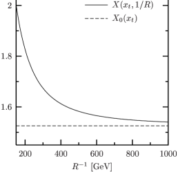
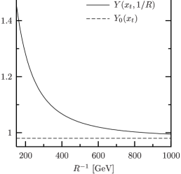
Figure 10: The functions (a) $X(x_{t},1/R)$ and $X_{0}(x_{t})$ and (b) $Y(x_{t},1/R)$ and $Y_{0}(x_{t})$.

In fig. 10 we plot $X(x_{t},1/R)$ and $Y(x_{t},1/R)$ versus $1/R$. We observe that due to the inequality $X_{0}>Y_{0}$ the relative impact of the KK modes is larger in the function $Y$. For $1/R=200\,{\rm GeV}$ the functions $X$ and $Y$ are enhanced by $20\%$ and $31\%$, respectively. For $1/R=250\,{\rm GeV}$ this enhancement decrease to $13\%(21\%)$ and are only $6\%(9\%)$ for $1/R=400\,{\rm GeV}$.

In table 2 we give the values of the functions $S$, $C$, $X$ and $Y$ for different $1/R$ and $m_{t}=167\,{\rm GeV}$.

$1/R~{}[{\rm GeV}]$	$S$	$C$	$X$	$Y$
$200$	$2.813$	$1.099$	$1.826$	$1.281$
$250$	$2.664$	$1.003$	$1.731$	$1.185$
$300$	$2.582$	$0.946$	$1.674$	$1.128$
$400$	$2.500$	$0.885$	$1.613$	$1.067$
SM	$2.398$	$0.798$	$1.526$	$0.980$

Table 2: Values for the functions $S$, $C$, $X$ and $Y$.

4.8 Branching Ratios for Rare Decays

The branching ratios for the rare decays in question can be directly obtained from [25] by simply replacing the SM functions $X_{0}$ and $Y_{0}$ by $X(x_{t},1/R)$ and $Y(x_{t},1/R)$, respectively. We have

$$Br(K^{+}\rightarrow\pi^{+}\nu\bar{\nu})=\kappa_{+}\cdot\left[\left({{\rm Im}\lambda_{t}\over\lambda^{5}}X(x_{t},1/R)\right)^{2}+\left({{\rm Re}\lambda_{c}\over\lambda}P_{0}(X)+{{\rm Re}\lambda_{t}\over\lambda^{5}}X(x_{t},1/R)\right)^{2}\right]~{},$$ (4.24)

$$\kappa_{+}=r_{K^{+}}{3\alpha^{2}Br(K^{+}\to\pi^{0}e^{+}\nu)\over 2\pi^{2}\sin^{4}\theta_{w}}\lambda^{8}=4.31\cdot 10^{-11}\,,$$ (4.25)

where we have used [52]

$$\alpha=\frac{1}{129},\qquad\sin^{2}\theta_{w}=0.23,\qquad Br(K^{+}\to\pi^{0}e^{+}\nu)=4.87\cdot 10^{-2}\,.$$ (4.26)

Here $\lambda_{i}=V^{\ast}_{is}V_{id}$ with $\lambda_{c}$ being real to a very high accuracy. $r_{K^{+}}=0.901$ summarizes isospin breaking corrections [53] in relating $K^{+}\rightarrow\pi^{+}\nu\bar{\nu}$ to $K^{+}\to\pi^{0}e^{+}\nu$. $P_{0}(X)$ is given in (4.7).

Next,

$$Br(K_{\rm L}\to\pi^{0}\nu\bar{\nu})=\kappa_{\rm L}\cdot\left({{\rm Im}\lambda_{t}\over\lambda^{5}}X(x_{t},1/R)\right)^{2}~{},$$ (4.27)

$$\kappa_{\rm L}=\frac{r_{K_{\rm L}}}{r_{K^{+}}}{\tau(K_{\rm L})\over\tau(K^{+})}\kappa_{+}=1.88\cdot 10^{-10}$$ (4.28)

with $\kappa_{+}$ given in (4.25) and $r_{K_{\rm L}}=0.944$ summarizing isospin breaking corrections in relating $K_{\rm L}\rightarrow\pi^{0}\nu\bar{\nu}$ to $K^{+}\to\pi^{0}e^{+}\nu$ [53].

Next, normalizing to $Br(B\to X_{c}e\bar{\nu})$ and summing over three neutrino flavours we find

$$\frac{Br(B\to X_{s}\nu\bar{\nu})}{Br(B\to X_{c}e\bar{\nu})}=\frac{3\alpha^{2}}{4\pi^{2}\sin^{4}\theta_{w}}\frac{|V_{ts}|^{2}}{|V_{cb}|^{2}}\frac{X^{2}(x_{t},1/R)}{f(z)}\frac{\kappa(0)}{\kappa(z)}\,.$$ (4.29)

Here $f(z)$ is the phase-space factor for $B\to X_{c}e\bar{\nu}$ with $z=m_{\rm c}^{2}/m_{\rm b}^{2}$ and $\kappa(z)=0.88$ [54, 55] is the corresponding QCD correction. The factor $\kappa(0)=0.83$ represents the QCD correction to the matrix element of the $b\to s\nu\bar{\nu}$ transition due to virtual and bremsstrahlung contributions. In the case of $B\to X_{d}\nu\bar{\nu}$ one has to replace $V_{ts}$ by $V_{td}$ which results in a decrease of the branching ratio by roughly an order of magnitude. In our numerical calculations we set $f(z)=0.54$ and $Br(B\to X_{c}e\bar{\nu})=0.104$.

Next, the branching ratio for $B_{s}\to l^{+}l^{-}$ is given by

$$Br(B_{s}\to l^{+}l^{-})=\tau(B_{s})\frac{G^{2}_{\rm F}}{\pi}\left(\frac{\alpha}{4\pi\sin^{2}\theta_{w}}\right)^{2}F^{2}_{B_{s}}m^{2}_{l}m_{B_{s}}\sqrt{1-4\frac{m^{2}_{l}}{m^{2}_{B_{s}}}}|V^{\ast}_{tb}V_{ts}|^{2}Y^{2}(x_{t},1/R)$$ (4.30)

where $F_{B_{s}}$ is the $B_{s}$ meson decay constant. The formula for $Br(B_{d}\to l^{+}l^{-})$ is obtained by replacing $s$ by $d$. The relevant input parameters are [32]

$$F_{B_{d}}=(203^{+27}_{-34})~{}{\rm MeV},\qquad F_{B_{s}}=(238\pm 31)~{}{\rm MeV}~{}.$$ (4.31)

We set also $\tau(B_{s})=1.46~{}{\rm ps}$ and $\tau(B_{d})=1.54~{}{\rm ps}$ [52]. The short distance contribution to the dispersive part of $K_{\rm L}\to\mu^{+}\mu^{-}$ is given by [46, 49]

$$Br(K_{\rm L}\to\mu^{+}\mu^{-})_{\rm SD}=\kappa_{\mu}\left[\frac{{\rm Re}\lambda_{c}}{\lambda}P_{0}(Y)+\frac{{\rm Re}\lambda_{t}}{\lambda^{5}}Y(x_{t},1/R)\right]^{2},$$ (4.32)

$$\kappa_{\mu}=\frac{\alpha^{2}Br(K^{+}\to\mu^{+}\nu)}{\pi^{2}\sin^{4}\theta_{w}}\frac{\tau(K_{\rm L})}{\tau(K^{+})}\lambda^{8}=1.733\cdot 10^{-9}\,,$$ (4.33)

where we have used $Br(K^{+}\to\mu^{+}\nu)=0.634$. The charm contribution including NLO corrections is given by [48]

$$P_{0}(Y)=\frac{Y_{\rm NL}}{\lambda^{4}}=0.128\pm 0.013.$$ (4.34)

Unfortunately due to long distance contributions to the dispersive part of $K_{L}\to\mu^{+}\mu^{-}$, the extraction of $Br(K_{\rm L}\to\mu^{+}\mu^{-})_{\rm SD}$ from the data is subject to considerable uncertainties. The present best estimate reads [56]

$$Br(K_{\rm L}\to\mu^{+}\mu^{-})_{\rm SD}\leq 2.5\cdot 10^{-9}~{}.$$ (4.35)

4.9 GIM Mechanism and Convergence of the KK Sum

The tree-level masses of the KK modes of all particles approach the value $n/R$ for large KK mode numbers $n$, see eq. (2.36) and (A.2). Due to the unitary CKM matrix the GIM mechanism [12] comes into play. It suppresses partly the higher KK mode contributions to the sums in eq. (3.4), (4.2), (4.5) and (4.10) and is essential for the determination of the dominant contributions. For the $S_{n}$ function the GIM suppression amounts to an additional factor of $1/n^{4}$ for the contributions ${WW}$, ${GG}$ and ${WG}$. The contributions from diagrams with $a^{\pm}$ are not suppressed due to the second term in the coupling $m_{4}^{(t)}$, see (A.3). This results in a hierarchy of the various contributions to $S_{n}$ with ${WW}$, ${GG}$ and ${WG}$ proportional to $1/n^{6}$, ${Wa}$ and ${Ga}$ proportional to $1/n^{4}$ and the dominant contribution ${aa}$ proportional to $1/n^{2}$ for large values of $n$.

For the penguin diagrams the effect of the GIM mechanism on the convergence of the particular contributions is partly hidden by the subtle cancellation of divergencies among the different contributions and the two self-energy diagrams. For the combinations plotted in fig. 8 we observe that the term corresponding to $W^{\pm}:F_{1}+F_{2}+F_{5}$ is logarithmically divergent without GIM and shows a $1/n^{2}$ behaviour after GIM mechanism has been taken into account. The $a^{\pm},G^{\pm}:F_{3}+F_{4}+F_{6}+F_{7}$ term shows no GIM suppression and is proportional to $1/n^{2}$ for large values of $n$. The mixed term $W^{\pm},a^{\pm},G^{\pm}:F_{8}$ is constant for large $n$ before the inclusion of GIM mechanism, but is GIM suppressed by a factor of $1/n^{2}$.

The contributions to $B^{\nu\bar{\nu}}_{n}$ and $B^{\mu\bar{\mu}}_{n}$ show a $1/n^{4}$ behaviour with and without GIM, except the $G_{WW}$ and $H_{WW}$ terms. They are proportional to $1/n^{2}$ without GIM and behave like $1/n^{4}$ with GIM suppression at work. This different asymptotic behaviour with respect to the $S_{n}$ function is due to the appearance of leptons with negligible zero-mode masses instead of quarks in the box diagrams contribution to the functions $G$ and $H$, see eq. (A.3).

4.10 Numerical Analysis

As discussed in section 3, $|V_{td}|$, $\bar{\varrho}$ and $\bar{\eta}$ in the SM and in the ACD model differ from each other. In our numerical analysis we will take this difference into account. Not taking this difference into account would misrepresent significantly the patterns of the enhancements of branching ratios in question.

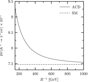
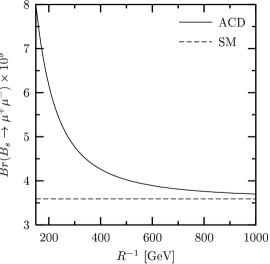
Figure 11: Branching ratio for the decays $K^{+}\rightarrow\pi^{+}\nu\overline{\nu}$ and $B_{s}\to\mu^{+}\mu^{-}$ as predicted by the ACD model and the SM as functions of the inverse radius $R$ of the extra dimension.

In fig. 11 we show the branching ratios $Br(K^{+}\rightarrow\pi^{+}\nu\bar{\nu})$ and $Br(B_{s}\to\mu^{+}\mu^{-})$ as functions of the compactification scale $1/R$. As $|V_{ts}|_{ACD}=|V_{ts}|_{SM}$, the enhancement of $Br(B_{s}\to\mu^{+}\mu^{-})$ is entirely governed by the ratio $(Y/Y_{0})^{2}$. On the other hand the dependence of $Br(K^{+}\rightarrow\pi^{+}\nu\bar{\nu})$ on $1/R$ differs from the one of $(X/X_{0})^{2}$ because of the additional charm contribution that is independent of $1/R$ and the fact that $V_{td}$ in the ACD model differs from its SM value. The remaining branching ratios are shown in table 3. The $1/R$ dependence of $Br(B\to X_{s}\nu\bar{\nu})$ is governed by the function $X^{2}(x_{t}/1/R)$, while the corresponding dependences of $Br(B\to X_{d}\nu\bar{\nu})$, $Br(K_{\rm L}\rightarrow\pi^{0}\nu\bar{\nu})$, $Br(B_{d}\to\mu^{+}\mu^{-})$ and $Br(K_{\rm L}\to\mu^{+}\mu^{-})_{\rm SD}$ include also the $1/R$ dependence of $V_{td}$ shown in fig. 4. As expected, all the branching ratios are significantly enhanced for $1/R\leq 300\,{\rm GeV}$. For $1/R\geq 400\,{\rm GeV}$, except for $Br(B_{s}\to\mu^{+}\mu^{-})$, the distinction between the predictions of the ACD model and the SM will be very difficult.

$1/R$	$200\,{\rm GeV}$	$250\,{\rm GeV}$	$300\,{\rm GeV}$	$400\,{\rm GeV}$	SM
$Br(K^{+}\rightarrow\pi^{+}\nu\bar{\nu})\times 10^{11}$	$8.70$	$8.36$	$8.13$	$7.88$	$7.49$
$Br(K_{\rm L}\rightarrow\pi^{0}\nu\bar{\nu})\times 10^{11}$	$3.26$	$3.17$	$3.09$	$2.98$	$2.80$
$Br(K_{\rm L}\to\mu^{+}\mu^{-})_{\rm SD}\times 10^{9}$	$1.10$	$1.00$	$0.95$	$0.88$	$0.79$
$Br(B\to X_{s}\nu\bar{\nu})\times 10^{5}$	$5.09$	$4.56$	$4.26$	$3.95$	$3.53$
$Br(B\to X_{d}\nu\bar{\nu})\times 10^{6}$	$1.80$	$1.70$	$1.64$	$1.58$	$1.47$
$Br(B_{s}\to\mu^{+}\mu^{-})\times 10^{9}$	$6.18$	$5.28$	$4.78$	$4.27$	$3.59$
$Br(B_{d}\to\mu^{+}\mu^{-})\times 10^{10}$	$1.56$	$1.41$	$1.32$	$1.22$	$1.07$

Table 3: Branching ratios for rare decays in the ACD model and the SM as discussed in the text.

In this numerical analysis we have used the results for the CKM parameters of fig. 4 and the central values of all the remaining input parameters as given above. The uncertainties in these parameters partly cover the differences between the ACD model and the SM model and it is essential to reduce these uncertainties considerably if one wants to see the effects of the KK modes in the branching ratios in question. Therefore a detailed analysis that includes all uncertainties would be in our opinion premature at present.

4.11 An Upper Bound on $Br(K^{+}\rightarrow\pi^{+}\nu\bar{\nu})$ in the ACD Model

The enhancement of $Br(K^{+}\rightarrow\pi^{+}\nu\bar{\nu})$ in the ACD model is interesting in view of the results from the AGS E787 collaboration at Brookhaven [57] that read

$$Br(K^{+}\rightarrow\pi^{+}\nu\bar{\nu})=(15.7^{+17.5}_{-8.2})\cdot 10^{-11}$$ (4.36)

with the central value by a factor of 2 above the SM expectation. Even if the errors are substantial and this result is compatible with the SM, the ACD model with a low compactification scale is closer to the data. As emphasized in [57, 58] the central value in (4.36) implies within the SM a value for $|V_{td}|$ that is substantially higher than the value obtained from the standard analysis of the UT of section 3. Here we would like to emphasize that within the ACD model $Br(K^{+}\rightarrow\pi^{+}\nu\bar{\nu})$ is closer to the data in spite of the fact that $|V_{td}|_{\rm ACD}<|V_{td}|_{\rm SM}$. The enhanced $Z^{0}$–vertex represented by the function $C$ is responsible for this behaviour.

In [48] an upper bound on $Br(K^{+}\rightarrow\pi^{+}\nu\bar{\nu})$ has been derived within the SM. This bound depends only on $|V_{cb}|$, $X_{0}$, $\xi$ and $\Delta M_{d}/\Delta M_{s}$. With the precise value for the angle $\beta$ now available this bound can be turned into a useful formula for $Br(K^{+}\rightarrow\pi^{+}\nu\bar{\nu})$ [58] that expresses this branching ratio in terms of theoretically clean observables. In the ACD model this formula reads:

$$Br(K^{+}\rightarrow\pi^{+}\nu\bar{\nu})=\bar{\kappa}_{+}|V_{cb}|^{4}X^{2}(x_{t},1/R)\left[\sigma R^{2}_{t}\sin^{2}\beta+\frac{1}{\sigma}\left(R_{t}\cos\beta+\frac{\lambda^{4}P_{0}(X)}{|V_{cb}|^{2}X(x_{t},1/R)}\right)^{2}\right],$$ (4.37)

where $\sigma=1/(1-\lambda^{2}/2)^{2}$, $\bar{\kappa}_{+}=\kappa_{+}/\lambda^{8}$ and $R_{t}$ is given in (3.29). This formula is theoretically very clean and does not involve hadronic uncertainties except for $\xi$ in (3.29) and to a lesser extent in $|V_{cb}|$.

In order to find the upper bound on $Br(K^{+}\rightarrow\pi^{+}\nu\bar{\nu})$ in the ACD model we use

$$|V_{cb}|\leq 0.0422~{},~{}\quad P_{0}(X)<0.47~{},~{}\quad\sin\beta=0.40~{},~{}\quad m_{\rm t}<172~{}\,{\rm GeV},$$ (4.38)

where we have set $\sin\beta$ to its central value (see (3.33)) as $Br(K^{+}\rightarrow\pi^{+}\nu\bar{\nu})$ depends very weakly on it. The bound on $|V_{cb}|$ results from $|V_{cb}|=0.0406\pm 0.0008$ [34]. We used here two standard deviations as the determination of $|V_{cb}|$ involves some hadronic uncertainties. The result of this exercise is shown in table 4. We give there $Br(K^{+}\rightarrow\pi^{+}\nu\bar{\nu})_{\rm max}$ as a function of $\xi$ and $1/R$ for two different values of $\Delta M_{s}$. The range for $\xi$ chosen by us is in accordance with (3.30) and the recent new analysis in [59] that gives $\xi=1.22\pm 0.07$. The upper bound in the SM given in the last column is lower than the values for $1/R=400~{}\,{\rm GeV}$ by roughly $10\%$. We observe that for $1/R=200~{}\,{\rm GeV}$ and $\xi=1.30$ the maximal value for $Br(K^{+}\rightarrow\pi^{+}\nu\bar{\nu})$ in the ACD model is rather close to the central value in (4.36).

At first sight the $30\%$ enhancement of $Br(K^{+}\rightarrow\pi^{+}\nu\bar{\nu})$ for $1/R=200\,{\rm GeV}$ with respect to the SM values seems to contradict the results in table 3, where a more modest enhancement of $Br(K^{+}\rightarrow\pi^{+}\nu\bar{\nu})$ is seen. However, one should realize that now $\Delta M_{d}/\Delta M_{s}$ and not $\Delta M_{d}$ alone enters the analysis and the enhancement of the function $X$ is not accompanied by a suppression of $|V_{td}|$, that with $R_{t}$ given by (3.29), equals the one in the SM. The consistency with the experimental value of $\Delta M_{d}$ requires then a sufficiently small $\sqrt{\hat{B}_{B_{d}}}F_{B_{d}}$. In table 4 we indicate by a star the cases that require $\sqrt{\hat{B}_{B_{d}}}F_{B_{d}}\leq 190\,{\rm MeV}$. Such low values are rather improbable in view of (3.30) and consequently values of $Br(K^{+}\rightarrow\pi^{+}\nu\bar{\nu})$ larger than $12\cdot 10^{-11}$ are rather unlikely even in the ACD model.

$\xi$	$1/R=200~{}\,{\rm GeV}$	$1/R=250~{}\,{\rm GeV}$	$1/R=300~{}\,{\rm GeV}$	$1/R=400~{}\,{\rm GeV}$	SM
$1.30$	$13.8^{*}~{}(12.3^{*})$	$12.7^{*}~{}(11.3^{*})$	$12.0^{*}~{}(10.7)$	$11.3^{*}~{}(10.1)$	$10.8~{}(9.3)$
$1.25$	$13.0^{*}~{}(11.6)$	$12.0~{}(10.7)$	$11.4~{}(10.2)$	$10.7~{}(9.6)$	$10.3~{}(8.8)$
$1.20$	$12.2^{*}~{}(10.9)$	$11.3~{}(10.1)$	$10.7~{}(9.6)$	$10.1~{}(9.1)$	$9.7~{}(8.4)$
$1.15$	$11.5~{}(10.3)$	$10.6~{}(9.5)$	$10.1~{}(9.0)$	$9.5~{}(8.5)$	$9.1~{}(7.9)$

Table 4: Upper bound on $Br(K^{+}\rightarrow\pi^{+}\nu\bar{\nu})$ in units of $10^{-11}$ for different values of $\xi$ and $1/R$ and $\Delta M_{s}=18/{\rm ps}~{}(21/{\rm ps})$. The stars indicate the results corresponding to $\sqrt{\hat{B}_{B_{d}}}F_{B_{d}}\leq 190\,{\rm MeV}$.

5 Summary and Outlook

In this paper we have calculated for the first time the contributions of the Kaluza-Klein (KK) modes to $\Delta M_{K}$, $\varepsilon_{K}$, $\Delta M_{d,s}$ and rare decays $K^{+}\rightarrow\pi^{+}\nu\bar{\nu}$, $K_{\rm L}\rightarrow\pi^{0}\nu\bar{\nu}$, $K_{\rm L}\to\mu^{+}\mu^{-}$, $B\to X_{s,d}\nu\bar{\nu}$ and $B_{s,d}\to\mu\bar{\mu}$ in the Appelquist, Cheng and Dobrescu (ACD) model with one universal extra dimension. As a byproduct we have given a list of the required Feynman rules that have not been presented in the literature so far.

The nice property of this extension of the SM is the presence of only a single new parameter, $1/R$. This economy in new parameters should be contrasted with supersymmetric theories and models with an extended Higgs sector. Taking $1/R=200~{}\,{\rm GeV}$ our findings are as follows:

• The short distance one-loop function $S(x_{t},1/R)$ relevant for $\Delta F=2$ transitions is larger than the corresponding SM function $S_{0}(x_{t})$ by roughly $17\%$. This implies on the basis of $\varepsilon_{K}$ and $\Delta M_{d}$ a $8\%$ suppression of $|V_{td}|_{\rm ACD}$ with respect to $|V_{td}|_{\rm SM}$ and a decrease of the angle $\gamma_{\rm ACD}$ by $10^{\circ}$ with respect to $\gamma_{\rm SM}$. On the other hand, $(\Delta M_{s})_{\rm ACD}$ is larger than $(\Delta M_{s})_{\rm SM}$ by $17\%$, see section 3 for details. $\Delta M_{K}$ is essentially uneffected.

• In order to see whether the modifications of the SM expectations are required by the data, the comparision of $|V_{td}|$ and $\gamma$ extracted from $\varepsilon_{K}$ and $\Delta M_{d}$ in the SM and in the ACD model with the universal unitarity triangle constructed by means of $|V_{ub}/V_{cb}|$, $\Delta M_{d}/\Delta M_{s}$ and $a(\psi K_{S})$ will be important. To this end, the data on these quantities have to be improved and the uncertainties in the relevant non-perturbative parameters reduced.

• The short distance one-loop function $X(x_{t},1/R)$ relevant for the decays $K^{+}\rightarrow\pi^{+}\nu\bar{\nu}$, $K_{\rm L}\rightarrow\pi^{0}\nu\bar{\nu}$ and $B\to X_{s,d}\nu\bar{\nu}$ is larger than the corresponding SM function $X_{0}(x_{t})$ by roughly $20\%$ due to KK contributions to the $Z^{0}$-penguins. In the case of $K^{+}\rightarrow\pi^{+}\nu\bar{\nu}$, $K_{\rm L}\rightarrow\pi^{0}\nu\bar{\nu}$ and $B\to X_{d}\nu\bar{\nu}$ this enhancement is partially compensated by the fact that $|V_{td}|_{\rm ACD}<|V_{td}|_{\rm SM}$ and $\bar{\eta}_{\rm ACD}<\bar{\eta}_{\rm SM}$. We then find the enhancements of $Br(K^{+}\rightarrow\pi^{+}\nu\bar{\nu})$, $Br(K_{\rm L}\rightarrow\pi^{0}\nu\bar{\nu})$ and $Br(B\to X_{d}\nu\bar{\nu})$ over the SM expectations by $16\%$, $17\%$ and $22\%$, respectively. As $B\to X_{s}\nu\bar{\nu}$ is governed by the CKM element $|V_{ts}|$ that is common to the SM and the ACD model, the enhancement of $Br(B\to X_{s}\nu\bar{\nu})$ amounts to $44\%$.

• The short distance one-loop function $Y(x_{t},1/R)$ relevant for the decays $B_{d,s}\to\mu\bar{\mu}$ and $K_{L}\to\mu\bar{\mu}$, is larger than the corresponding SM function $Y_{0}(x_{t})$ by roughly $30\%$. As $B_{s}\to\mu\bar{\mu}$ is governed by the CKM element $|V_{ts}|$ with $|V_{ts}|_{\rm ACD}=|V_{ts}|_{\rm SM}$ this implies a $72\%$ enhancement of $Br(B_{s}\to\mu\bar{\mu})$ relative to the SM expectation. In the case of $B_{d}\to\mu\bar{\mu}$ and $K_{L}\to\mu\bar{\mu}$, due to $|V_{td}|_{\rm ACD}<|V_{td}|_{\rm SM}$, the corresponding enhancements amount to $38\%$ and $46\%$.

• As the ACD model belongs to the class of MFV models, general properties of these models identified in [14, 60] are automatically valid here.

• For $1/R=250~{}(300)~{}\,{\rm GeV}$ all these effects are decreased roughly by a factor of $1.5~{}(2.0)$. See fig. 11 and table 3.

In short, the signatures of the deviations from the SM expectations are:

• The decrease of $|V_{td}|$, $\gamma$, $\bar{\eta}$ and $\bar{\varrho}$.

• The increase of $\Delta M_{s}$.

• The increase of all branching ratios considered in this paper with a hierarchical structure of maximal enhancements: $K^{+}\rightarrow\pi^{+}\nu\bar{\nu}~{}(16\%)$, $K_{\rm L}\rightarrow\pi^{0}\nu\bar{\nu}~{}(17\%)$, $B\to X_{d}\nu\bar{\nu}~{}(22\%)$, $K_{L}\to\mu\bar{\mu}~{}(38\%)$, $B\to X_{s}\nu\bar{\nu}~{}(44\%)$, $B_{d}\to\mu\bar{\mu}~{}(46\%)$ and $B_{s}\to\mu\bar{\mu}~{}(72\%)$ for $1/R=200\,{\rm GeV}$. For $1/R=250~{}(300)\,{\rm GeV}$ these enhancements are decreased roughly by a factor of $1.5~{}(2.0)$.

In the coming years of particular interest will be the improved measurements of $Br(K^{+}\to\pi^{+}\nu\bar{\nu})$ and $\Delta M_{s}$. Indeed, in the MFV models $Br(K^{+}\to\pi^{+}\nu\bar{\nu})$ can be predicted as a function of $X$ once the angle $\beta$ and $\Delta M_{d}/\Delta M_{s}$ are known. The relevant formula is given in (4.37). For a given value of $X$, the branching ratio $Br(K^{+}\to\pi^{+}\nu\bar{\nu})$ decreases with increasing $\Delta M_{s}$. If the present central experimental values for $Br(K^{+}\to\pi^{+}\nu\bar{\nu})$ will remain while the experimental error will decrease significantly, the SM expectations for $Br(K^{+}\to\pi^{+}\nu\bar{\nu})$ will be significantly below the experimental data while the corresponding estimates within the ACD model may agree with them due to $X(x_{t},1/R)>X_{0}(x_{t})$, see table 4.

Another definite prediction of the ACD model is an increase of $\Delta M_{s}$ over the SM value. This should be contrasted with the prediction of the MSSM at large $\tan\beta$ where a suppression of $\Delta M_{s}$ with respect to the SM value is predicted [61]. Thus, when the ratio $(\Delta M_{s})_{\rm exp}/(\Delta M_{s})_{\rm SM}$ will be known with a sufficient accuracy, we will know whether the ACD model with a low $1/R$ or the MSSM with a large $\tan\beta$ is ruled out by the data.

A distinction between the ACD model and the MSSM at low $\tan\beta$ will also be possible. In the latter case the supersymmetric effects in $\Delta F=2$ transitions considered in section 3 are generally larger than in $\Delta F=1$ transions so that the branching ratios for $K^{+}\rightarrow\pi^{+}\nu\bar{\nu}$, $K_{\rm L}\rightarrow\pi^{0}\nu\bar{\nu}$, $K_{\rm L}\to\mu^{+}\mu^{-}$, $B\to X_{d}\nu\bar{\nu}$ and $B_{d}\to\mu\bar{\mu}$ are generally suppressed with respect to the SM while they can be enhanced for special ranges of supersymmetric parameters in the case of $B\to X_{s}\nu\bar{\nu}$ and $B_{s}\to\mu\bar{\mu}$ [62].

However, the main message from our analysis is the following one. Even for the lowest compactification scale, $1/R=200~{}\,{\rm GeV}$, considered by us, the ACD model is consistent with all the available data on FCNC processes analyzed here . No fine tunning of the parameters characteristic in the flavour sector for general supersymmetric models is necessary. This is first of all connected with the GIM mechanism that assures the convergence of the sum over the KK modes in the case of $Z^{0}$ penguin diagrams, removing the sensitivity of the calculated branching ratios to the scale $M_{s}\gg 1/R$ at which the higher dimensional theory becomes non-perturbative and at which the towers of the KK particles must be cut off in an appropriate way.

With the much improved data on the processes calculated in this paper and the theoretical uncertainties reduced, it should be possible in the future to distinguish the predictions of the ACD model from the SM ones, provided $1/R<400\,{\rm GeV}$. For higher compactification scales this distinction will be very difficult with a possible exception of $B_{s}\to\mu^{+}\mu^{-}$. Whether these findings apply also to $B\to X_{s}\gamma$, $B\to X_{s}l^{+}l^{-}$ and $K_{L}\to\pi^{0}e^{+}e^{-}$ is an interesting question. As the $Z^{0}$-penguins are enhanced in the ACD model, the corresponding enhancement of the branching ratios for $B\to X_{s}l^{+}l^{-}$ and $K_{L}\to\pi^{0}e^{+}e^{-}$ can easily be calculated by means of the known formulae [25, 63, 64]. However, such an analysis would clearly be unsatisfactory as these decays receive also contributions from the $\gamma$-penguins and magnetic penguins. The KK contributions to $\gamma$-penguins are unknown, while the corresponding contributions to the magnetic penguins have been calculated in the context of an analysis of the decay $B\to X_{s}\gamma$ under the assumption of the dominance of the scalars $a^{\pm}_{(n)}$ [2]. We have seen that this assumption would be correct in the case of $S(x_{t},1/R)$ for $1/R\geq 300\,{\rm GeV}$, but certainly would misrepresent the KK contributions to $C(x_{t},1/R)$ in view of strong cancellations between different contributions as discussed in section 4. Consequently a satisfactory analysis of $B\to X_{s}\gamma$, $B\to X_{s}l^{+}l^{-}$ and $K_{L}\to\pi^{0}e^{+}e^{-}$ requires a priori the inclusion of all KK contributions. We will address all these issues in the forthcoming paper [11].

Appendix A Feynman Rules in the ACD Model

In this section, we list all propagators and vertex rules needed for the calculation of the box and penguin diagrams considered in this paper. The Feynman rules are derived in the 5d $R_{\xi}$-gauge described in Section 2.3.

It is convenient to define a 4 dimensional counterpart to every parameter in the 5 dimensional Lagrangian, marked there with a caret. The conversion factors are chosen in order to eliminate all explicit appearances of factors of $\sqrt{2\pi R}$ in the Feynman rules:

$$\mu =\hat{\mu}, \hskip 60.27759ptv =\sqrt{2\pi R}~{}\hat{v}, \hskip 60.27759ptg_{2} =\frac{1}{\sqrt{2\pi R}}~{}\hat{g}_{2},$$ (A.1)

$$g^{\prime} =\frac{1}{\sqrt{2\pi R}}~{}\hat{g}^{\prime}, \lambda_{\mathcal{U}/\mathcal{D}} =\frac{1}{\sqrt{2\pi R}}~{}\hat{\lambda}_{\mathcal{U}/\mathcal{D}},$$

where $\hat{\mu}$ is the Higgs mass parameter.

In order to simplify the notation, we omit the KK indices of the fields and of the mass parameters defined in (A.3) and (A.4). There is no ambiguity because in one-loop calculations at least one field is always a zero-mode. In our case, this is the $Z$ boson in the $Z$ vertices, and the down-type quark or the neutrino in all other vertices. Due to KK parity conservation, the other two fields have equal KK mode number, i.e. either zero or $n\geq 1$.

Fermion zero-modes have substantially different Feynman rules than their KK excitations. The fields $\mathcal{Q}_{u}$, $\mathcal{Q}_{d}$, $\mathcal{U}$, $\mathcal{D}$, $\mathcal{L}_{\nu}$, $\mathcal{L}_{e}$ and $\mathcal{E}$ are always supposed to be $(n\geq 1)$-modes, while the zero-modes are labeled $u$, $d$, $\nu$ and $e$. The generation indices are $i=u,c,t$ and $j=d,s,b$ for the quarks and $i,j=e,\mu,\tau$ for the leptons.

The masses of all bosonic particles can be expressed in terms of four independent mass parameters:

$$M_{A(n)}^{2} =\frac{n^{2}}{R^{2}},$$ (A.2)

$$M_{Z(n)}^{2} =\frac{n^{2}}{R^{2}}+M^{2}_{Z},$$

$$M_{W(n)}^{2} =\frac{n^{2}}{R^{2}}+M^{2}_{W},$$

$$M_{H(n)}^{2} =\frac{n^{2}}{R^{2}}+2\mu^{2}.$$

We introduce two sets of mass parameters appearing in the fermion-scalar couplings. The mass parameters $m_{x}^{(i)}$ are

$$m_{1}^{(i)} =\frac{n}{R}c_{i(n)}+m_{i}s_{i(n)},$$ (A.3)

$$m_{2}^{(i)} =-\frac{n}{R}s_{i(n)}+m_{i}c_{i(n)},$$

$$m_{3}^{(i)} =-M_{W}c_{i(n)}+\frac{n}{R}\frac{m_{i}}{M_{W}}s_{i(n)},$$

$$m_{4}^{(i)} =M_{W}s_{i(n)}+\frac{n}{R}\frac{m_{i}}{M_{W}}c_{i(n)},$$

where $M_{W}$ and the up-type fermion masses $m_{i}$ on the r.h.s. are the zero-mode masses. The parameters $c_{i(n)}$ and $s_{i(n)}$ denote the cosine and sine respectively of the fermion mass mixing angle $\alpha_{i(n)}$ defined in (2.35). The mass parameters $M_{x}^{(i,j)}$ are

$$M_{1}^{(i,j)} =m_{j}c_{i(n)},$$ (A.4)

$$M_{2}^{(i,j)} =m_{j}s_{i(n)},$$

$$M_{3}^{(i,j)} =\frac{n}{R}\frac{m_{j}}{M_{W}}c_{i(n)},$$

$$M_{4}^{(i,j)} =\frac{n}{R}\frac{m_{j}}{M_{W}}s_{i(n)},$$

where again $M_{W}$ and the down-type fermion masses $m_{j}$ on the r.h.s. are the zero-mode masses.

All momenta and fields are assumed to be incoming.

A.1 Propagators

The propagators are:

for scalar fields $S=H,a^{0},a^{\pm},A_{5},G^{0},G^{\pm}$:

$\displaystyle=\frac{i}{k^{2}-M^{2}+i\epsilon},$

with the masses

$$\begin{array}[]{|c|cccccc|}\hline\cr S&H_{(n)}&a^{0}_{(n)}&a^{\pm}_{(n)}&A_{5(n)}&G^{0}_{(n)}&G^{\pm}_{(n)}\\ \hline\cr M&M_{H(n)}&M_{Z(n)}&M_{W(n)}&\sqrt{\xi}M_{A(n)}&\sqrt{\xi}M_{Z(n)}&\sqrt{\xi}M_{W(n)}\\ \hline\cr\end{array}$$ (A.5)

for gauge bosons $V=A,Z,W^{\pm}$:

$\displaystyle=\frac{-i}{k^{2}-M^{2}+i\epsilon}\left(g^{\mu\nu}-(1-\xi)\frac{k^{\mu}k^{\nu}}{k^{2}-\xi M^{2}+i\epsilon}\right),$

with the masses

$$\begin{array}[]{|c|ccc|}\hline\cr V&A_{(n)}&Z_{(n)}&W^{\pm}_{(n)}\\ \hline\cr M&M_{A(n)}&M_{Z(n)}&M_{W(n)}\\ \hline\cr\end{array}$$ (A.6)

for fermion fields $F=u,d,\mathcal{Q}_{u},\mathcal{Q}_{d},\mathcal{U},\mathcal{D},\nu,e,\mathcal{L}_{\nu},\mathcal{L}_{e},\mathcal{E}$:

$\displaystyle=\frac{i\left(k\!\!\!/+m\right)}{k^{2}-m^{2}+i\epsilon},$

with the masses

$$\begin{array}[]{|c|ccccccccccc|}\hline\cr F&u&d&\mathcal{Q}_{u(n)}&\mathcal{Q}_{d(n)}&\mathcal{U}_{(n)}&\mathcal{D}_{(n)}&\nu&e&\mathcal{L}_{\nu(n)}&\mathcal{L}_{e(n)}&\mathcal{E}_{(n)}\\ \hline\cr m&m_{u}&m_{d}&m_{u(n)}&m_{d(n)}&m_{u(n)}&m_{d(n)}&m_{\nu}&m_{e}&m_{\nu(n)}&m_{e(n)}&m_{e(n)}\\ \hline\cr\end{array}$$ (A.7)

A.2 Vertices

The Feynman rules for the vertices are:

$\displaystyle=\frac{g_{2}}{c_{w}M_{W(n)}}g_{\mu\nu}C.$

$$ZW^{+}G^{-} \;:\quad C =-s_{w}^{2}M_{W}^{2}+c_{w}^{2}\frac{n^{2}}{R^{2}},$$ (A.8)

$$ZW^{-}G^{+} \;:\quad C =s_{w}^{2}M_{W}^{2}-c_{w}^{2}\frac{n^{2}}{R^{2}},$$ (A.9)

$$ZW^{+}a^{-} \;:\quad C =-M_{W}\frac{n}{R},$$ (A.10)

$$ZW^{-}a^{+} \;:\quad C =M_{W}\frac{n}{R}.$$ (A.11)

$\displaystyle=\frac{ig_{2}}{2c_{w}M_{W(n)}^{2}}(k_{2}-k_{1})_{\mu}C.$

$$ZG^{+}G^{-} \;:\quad C =-\left(c_{w}^{2}-s_{w}^{2}\right)M_{W}^{2}-2c_{w}^{2}\frac{n^{2}}{R^{2}},$$ (A.12)

$$Za^{+}a^{-} \;:\quad C =-2c_{w}^{2}M_{W}^{2}-\left(c_{w}^{2}-s_{w}^{2}\right)\frac{n^{2}}{R^{2}},$$ (A.13)

$$ZG^{+}a^{-} \;:\quad C =M_{W}\frac{n}{R},$$ (A.14)

$$ZG^{-}a^{+} \;:\quad C =-M_{W}\frac{n}{R}.$$ (A.15)

$\displaystyle=ig_{2}c_{w}\bigl{(}g_{\mu\nu}(k_{2}-k_{1})_{\lambda}+g_{\mu\lambda}(k_{1}-k_{3})_{\nu}+g_{\lambda\nu}(k_{3}-k_{2})_{\mu}\bigr{)}.$

(A.16)

$\displaystyle=\frac{ig_{2}}{6c_{w}}\gamma_{\mu}\left(P_{L}C_{L}+P_{R}C_{R}\right).$

$$Z\overline{u}_{i}u_{i} \;:\quad \left\{\begin{array}[]{l}C_{L}=3-4s_{w}^{2},\\ C_{R}=-4s_{w}^{2},\end{array}\right. Z\overline{d}_{j}d_{j} \;:\quad \left\{\begin{array}[]{l}C_{L}=-3+2s_{w}^{2},\\ C_{R}=2s_{w}^{2},\end{array}\right.$$ (A.21)

$$Z\overline{\nu}_{i}\nu_{i} \;:\quad \left\{\begin{array}[]{l}C_{L}=3,\\ C_{R}=0,\end{array}\right. Z\overline{e}_{j}e_{j} \;:\quad \left\{\begin{array}[]{l}C_{L}=-3+6s_{w}^{2},\\ C_{R}=6s_{w}^{2},\end{array}\right.$$ (A.26)

$$Z\overline{\mathcal{Q}}_{i}\mathcal{Q}_{i} \;:\quad \left\{\begin{array}[]{l}C_{L}=-4s_{w}^{2}+3c_{i(n)}^{2},\\ C_{R}=-4s_{w}^{2}+3c_{i(n)}^{2},\end{array}\right. Z\overline{\mathcal{U}}_{i}\mathcal{U}_{i} \;:\quad \left\{\begin{array}[]{l}C_{L}=-4s_{w}^{2}+3s_{i(n)}^{2},\\ C_{R}=-4s_{w}^{2}+3s_{i(n)}^{2},\end{array}\right.$$ (A.31)

$$Z\overline{\mathcal{Q}}_{i}\mathcal{U}_{i} \;:\quad \left\{\begin{array}[]{l}C_{L}=-3s_{i(n)}c_{i(n)},\\ C_{R}=3s_{i(n)}c_{i(n)},\end{array}\right. Z\overline{\mathcal{U}}_{i}\mathcal{Q}_{i} \;:\quad \left\{\begin{array}[]{l}C_{L}=-3s_{i(n)}c_{i(n)},\\ C_{R}=3s_{i(n)}c_{i(n)}.\end{array}\right.$$ (A.36)

$\displaystyle=\frac{ig_{2}}{\sqrt{2}}\gamma_{\mu}P_{L}C_{L}.$

$$W^{+}~{}\overline{u}_{i}d_{j} \;:\quad C_{L} =V_{ij}, W^{-}~{}\overline{d}_{j}u_{i} \;:\quad C_{L} =V_{ij}^{*},$$ (A.37)

$$W^{+}~{}\overline{\mathcal{Q}}_{i}d_{j} \;:\quad C_{L} =c_{i(n)}V_{ij}, W^{-}~{}\overline{d}_{j}\mathcal{Q}_{i} \;:\quad C_{L} =c_{i(n)}V_{ij}^{*},$$ (A.38)

$$W^{+}~{}\overline{\mathcal{U}}_{i}d_{j} \;:\quad C_{L} =-s_{i(n)}V_{ij}, W^{-}~{}\overline{d}_{j}\mathcal{U}_{i} \;:\quad C_{L} =-s_{i(n)}V_{ij}^{*},$$ (A.39)

$$W^{+}~{}\overline{\nu}_{i}e_{j} \;:\quad C_{L} =\delta_{ij}, W^{-}~{}\overline{e}_{j}\nu_{i} \;:\quad C_{L} =\delta_{ij},$$ (A.40)

$$W^{+}~{}\overline{\nu}_{i}\mathcal{L}_{j} \;:\quad C_{L} =\delta_{ij}, W^{-}~{}\overline{\mathcal{L}}_{j}\nu_{i} \;:\quad C_{L} =\delta_{ij},$$ (A.41)

$$W^{+}~{}\overline{\nu}_{i}\mathcal{E}_{j} \;:\quad C_{L} =0, W^{-}~{}\overline{\mathcal{E}}_{j}\nu_{i} \;:\quad C_{L} =0.$$ (A.42)

$\displaystyle=\frac{g_{2}}{\sqrt{2}M_{W(n)}}(P_{L}C_{L}+P_{R}C_{R}).$

$$G^{+}~{}\overline{u}_{i}d_{j} \;:\quad \left\{\begin{array}[]{l}C_{L}=-m_{i}V_{ij},\\ C_{R}=m_{j}V_{ij},\end{array}\right. G^{-}~{}\overline{d}_{j}u_{i} \;:\quad \left\{\begin{array}[]{l}C_{L}=-m_{j}V_{ij}^{*},\\ C_{R}=m_{i}V_{ij}^{*},\end{array}\right.$$ (A.47)

$$G^{+}~{}\overline{\mathcal{Q}}_{i}d_{j} \;:\quad \left\{\begin{array}[]{l}C_{L}=-m_{1}^{(i)}V_{ij},\\ C_{R}=M_{1}^{(i,j)}V_{ij},\end{array}\right. G^{-}~{}\overline{d}_{j}\mathcal{Q}_{i} \;:\quad \left\{\begin{array}[]{l}C_{L}=-M_{1}^{(i,j)}V_{ij}^{*},\\ C_{R}=m_{1}^{(i)}V_{ij}^{*},\end{array}\right.$$ (A.52)

$$G^{+}~{}\overline{\mathcal{U}}_{i}d_{j} \;:\quad \left\{\begin{array}[]{l}C_{L}=m_{2}^{(i)}V_{ij},\\ C_{R}=-M_{2}^{(i,j)}V_{ij},\end{array}\right. G^{-}~{}\overline{d}_{j}\mathcal{U}_{i} \;:\quad \left\{\begin{array}[]{l}C_{L}=M_{2}^{(i,j)}V_{ij}^{*},\\ C_{R}=-m_{2}^{(i)}V_{ij}^{*},\end{array}\right.$$ (A.57)

$$G^{+}~{}\overline{\nu}_{i}e_{j} \;:\quad \left\{\begin{array}[]{l}C_{L}=0,\\ C_{R}=m_{j}\delta_{ij},\end{array}\right. G^{-}~{}\overline{e}_{j}\nu_{i} \;:\quad \left\{\begin{array}[]{l}C_{L}=-m_{j}\delta_{ij},\\ C_{R}=0,\end{array}\right.$$ (A.62)

$$G^{+}~{}\overline{\nu}_{i}\mathcal{L}_{j} \;:\quad \left\{\begin{array}[]{l}C_{L}=0,\\ C_{R}=m_{1}^{(j)}\delta_{ij},\end{array}\right. G^{-}~{}\overline{\mathcal{L}}_{j}\nu_{i} \;:\quad \left\{\begin{array}[]{l}C_{L}=-m_{1}^{(j)}\delta_{ij},\\ C_{R}=0,\end{array}\right.$$ (A.67)

$$G^{+}~{}\overline{\nu}_{i}\mathcal{E}_{j} \;:\quad \left\{\begin{array}[]{l}C_{L}=0,\\ C_{R}=-m_{2}^{(j)}\delta_{ij},\end{array}\right. G^{-}~{}\overline{\mathcal{E}}_{j}\nu_{i} \;:\quad \left\{\begin{array}[]{l}C_{L}=m_{2}^{(j)}\delta_{ij},\\ C_{R}=0,\end{array}\right.$$ (A.72)

$$a^{+}~{}\overline{\mathcal{Q}}_{i}d_{j} \;:\quad \left\{\begin{array}[]{l}C_{L}=-m_{3}^{(i)}V_{ij},\\ C_{R}=M_{3}^{(i,j)}V_{ij},\end{array}\right. a^{-}~{}\overline{d}_{j}\mathcal{Q}_{i} \;:\quad \left\{\begin{array}[]{l}C_{L}=-M_{3}^{(i,j)}V_{ij}^{*},\\ C_{R}=m_{3}^{(i)}V_{ij}^{*},\end{array}\right.$$ (A.77)

$$a^{+}~{}\overline{\mathcal{U}}_{i}d_{j} \;:\quad \left\{\begin{array}[]{l}C_{L}=m_{4}^{(i)}V_{ij},\\ C_{R}=-M_{4}^{(i,j)}V_{ij},\end{array}\right. a^{-}~{}\overline{d}_{j}\mathcal{U}_{i} \;:\quad \left\{\begin{array}[]{l}C_{L}=M_{4}^{(i,j)}V_{ij}^{*},\\ C_{R}=-m_{4}^{(i)}V_{ij}^{*},\end{array}\right.$$ (A.82)

$$a^{+}~{}\overline{\nu}_{i}\mathcal{L}_{j} \;:\quad \left\{\begin{array}[]{l}C_{L}=0,\\ C_{R}=m_{3}^{(j)}\delta_{ij},\end{array}\right. a^{-}~{}\overline{\mathcal{L}}_{j}\nu_{i} \;:\quad \left\{\begin{array}[]{l}C_{L}=-m_{3}^{(j)}\delta_{ij},\\ C_{R}=0,\end{array}\right.$$ (A.87)

$$a^{+}~{}\overline{\nu}_{i}\mathcal{E}_{j} \;:\quad \left\{\begin{array}[]{l}C_{L}=0,\\ C_{R}=-m_{4}^{(j)}\delta_{ij},\end{array}\right. a^{-}~{}\overline{\mathcal{E}}_{j}\nu_{i} \;:\quad \left\{\begin{array}[]{l}C_{L}=m_{4}^{(j)}\delta_{ij},\\ C_{R}=0.\end{array}\right.$$ (A.92)

Appendix B Different Contributions to $\Delta F=2$ Box Diagrams

The contributions from different sets of diagrams to the functions $F(x_{t(n)},x_{u(n)})$ in (3.8) are given as follows

$$F_{WW(n)}=\frac{M_{W}^{2}}{M_{W(n)}^{2}}~{}U(x_{t(n)},x_{u(n)}),$$ (B.1)

$$F_{WG(n)}=-2\frac{M_{W}^{2}m_{t(n)}m_{u(n)}}{M_{W(n)}^{6}}\left[m_{1}^{(t)}c_{t(n)}+m_{2}^{(t)}s_{t(n)}\right]\left[m_{1}^{(u)}c_{u(n)}+m_{2}^{(u)}s_{u(n)}\right]$$ (B.2)

$${}\times\tilde{U}(x_{t(n)},x_{u(n)}),$$

$$F_{Wa(n)}=-2\frac{M_{W}^{2}m_{t(n)}m_{u(n)}}{M_{W(n)}^{6}}\left[m_{3}^{(t)}c_{t(n)}+m_{4}^{(t)}s_{t(n)}\right]\left[m_{3}^{(u)}c_{u(n)}+m_{4}^{(u)}s_{u(n)}\right]$$ (B.3)

$${}\times\tilde{U}(x_{t(n)},x_{u(n)}),$$

$$F_{Ga(n)}=\frac{1}{2}\frac{M_{W}^{2}}{M_{W(n)}^{6}}\left[m_{1}^{(t)}m_{3}^{(t)}+m_{2}^{(t)}m_{4}^{(t)}\right]\left[m_{1}^{(u)}m_{3}^{(u)}+m_{2}^{(u)}m_{4}^{(u)}\right]$$ (B.4)

$${}\times U(x_{t(n)},x_{u(n)}),$$

$$F_{GG(n)}=\frac{1}{4}\frac{M_{W}^{2}}{M_{W(n)}^{6}}\left[(m_{1}^{(t)})^{2}+(m_{2}^{(t)})^{2}\right]\left[(m_{1}^{(u)})^{2}+(m_{2}^{(u)})^{2}\right]U(x_{t(n)},x_{u(n)}),$$ (B.5)

$$F_{aa(n)}=\frac{1}{4}\frac{M_{W}^{2}}{M_{W(n)}^{6}}\left[(m_{3}^{(t)})^{2}+(m_{4}^{(t)})^{2}\right]\left[(m_{3}^{(u)})^{2}+(m_{4}^{(u)})^{2}\right]U(x_{t(n)},x_{u(n)}).$$ (B.6)

The functions $U$ and $\tilde{U}$ are defined as follows

$$U(x_{t},x_{u})=\frac{x_{t}^{2}\log{x_{t}}}{(x_{t}-x_{u})(1-x_{t})^{2}}+\frac{x_{u}^{2}\log{x_{u}}}{(x_{u}-x_{t})(1-x_{u})^{2}}+\frac{1}{(1-x_{u})(1-x_{t})},$$ (B.7)

$$U(x_{t},x_{t})=\frac{2x_{t}\log{x_{t}}}{(1-x_{t})^{3}}+\frac{1+x_{t}}{(1-x_{t})^{2}},$$ (B.8)

$$\tilde{U}(x_{t},x_{u})=\frac{x_{t}\log{x_{t}}}{(x_{t}-x_{u})(1-x_{t})^{2}}+\frac{x_{u}\log{x_{u}}}{(x_{u}-x_{t})(1-x_{u})^{2}}+\frac{1}{(1-x_{u})(1-x_{t})},$$ (B.9)

$$\tilde{U}(x_{t},x_{t})=\frac{(1+x_{t})\log{x_{t}}}{(1-x_{t})^{3}}+\frac{2}{(1-x_{t})^{2}}.$$ (B.10)

Appendix C Different Contributions to $Z^{0}$-Penguin Diagrams

The contributions of the diagrams in fig. 7 to the functions $F(x_{f})$ in (4.12) are given as follows

$$F_{1}(x_{f(n)}) = \frac{1}{8}\left(c_{f(n)}^{4}+s_{f(n)}^{4}-\frac{4}{3}s_{w}^{2}\right)$$ (C.1)

$$\times\left[\Delta+\ln\frac{\mu^{2}}{m^{2}_{f(n)}}+h_{q}\left(x_{f(n)}\right)-\frac{3}{2}-2x_{f(n)}h_{q}\left(x_{f(n)}\right)\right],$$

$$F_{2}(x_{f(n)}) = \frac{1}{4}c_{f(n)}^{2}s_{f(n)}^{2}\left[\Delta+\ln\frac{\mu^{2}}{m_{f(n)}^{2}}-\frac{3}{2}+h_{q}\left(x_{f(n)}\right)+2x_{f(n)}h_{q}\left(x_{f(n)}\right){}\right],$$ (C.2)

$$F_{3}(x_{f(n)}) = \frac{\displaystyle 1}{\displaystyle 16m^{2}_{W(n)}}\left[\left((m^{{(f)}}_{1})^{2}+(m^{{(f)}}_{3})^{2}\right)\left(c_{f{(n)}}^{2}-\frac{4}{3}s_{w}^{2}\right)+\left((m^{{(f)}}_{2})^{2}+(m^{{(f)}}_{4})^{2}\right)\left(s_{f(n)}^{2}-\frac{4}{3}s_{w}^{2}\right)\right]$$ (C.3)

$$\times\left[\Delta+\ln\frac{\mu^{2}}{m_{f(n)}^{2}}-\frac{1}{2}+h_{q}\left(x_{f(n)}\right)-2x_{f(n)}h_{q}\left(x_{f(n)}\right)\right],$$

$$F_{4}(x_{f(n)}) = -\frac{1}{8M^{2}_{W(n)}}\left(m^{{(f)}}_{1}\,m^{{(f)}}_{2}+m^{{(f)}}_{3}\,m^{{(f)}}_{4}\right)~{}c_{f(n)}~{}s_{f(n)}$$ (C.4)

$$\times\left[\Delta+\ln\frac{\mu^{2}}{m_{f(n)}^{2}}-\frac{1}{2}+h_{q}\left(x_{f(n)}\right)+2x_{f(n)}h_{q}\left(x_{f(n)}\right)\right],$$

$$F_{5}(x_{f(n)}) = -\frac{3}{4}\,c_{w}^{2}\,\left[\Delta+\ln\frac{\mu^{2}}{M_{W(n)}^{2}}-\frac{1}{6}-x_{f(n)}h_{w}\left(x_{f(n)}\right)\right],$$ (C.5)

$$F_{6}(x_{f(n)}) = -\frac{1}{16\,m^{4}_{W(n)}}\left[\left(\left(1-2\,s_{w}^{2}\right)M_{W}^{2}+2c_{w}^{2}\frac{n^{2}}{R^{2}}\right)\left((m^{{(f)}}_{1})^{2}+(m^{{(f)}}_{2})^{2}\right)\right.$$ (C.6)

$$\left.+\left(\left(1-2\,s_{w}^{2}\right)\frac{n^{2}}{R^{2}}+2c_{w}^{2}M_{W}^{2}\right)\left((m^{{(f)}}_{3})^{2}+(m^{{(f)}}_{4})^{2}\right)\right]$$

$$\times\left[\Delta+\ln\frac{\mu^{2}}{M_{W(n)}^{2}}+\frac{1}{2}-x_{f(n)}h_{w}\left(x_{f(n)}\right)\right],$$

$$F_{7}(x_{f(n)}) = \frac{M_{W}}{8M^{4}_{W{(n)}}}\frac{n}{R}\left(m^{{(f)}}_{1}m^{{(f)}}_{3}+m^{{(f)}}_{2}m^{{(f)}}_{4}\right)$$ (C.7)

$$\times\left[\Delta+\ln\frac{\mu^{2}}{M_{W(n)}^{2}}+\frac{1}{2}-x_{f(n)}\,h_{w}\left(x_{f(n)}\right)\right],$$

$$F_{8}(x_{f(n)}) = \,\frac{m_{f(n)}}{2M^{4}_{W{(n)}}}\left[\left(s_{w}^{2}M_{W}^{2}-c_{w}^{2}\frac{n^{2}}{R^{2}}\right)\,\left(m^{{(f)}}_{1}~{}c_{f(n)}+m^{{(f)}}_{2}~{}s_{f(n)}\right)\right.$$ (C.8)

$$\left.+M_{W}{n\over R}\,\left(m^{{(f)}}_{3}~{}c_{f(n)}+m^{{(f)}}_{4}~{}s_{f(n)}\right)\right]\,h_{w}\left(x_{f(n)}\right).$$

Here

$$\Delta=\frac{1}{\epsilon}+\ln 4\pi-\gamma_{E},\qquad D=4-2\epsilon$$ (C.9)

and the functions $h_{q}$ and $h_{w}$ are given by:

$$h_{q}(x) = \frac{1}{1-x}+\frac{\ln x}{(1-x)^{2}},$$ (C.10)

$$h_{w}(x) = \frac{1}{1-x}+\frac{x\ln x}{(1-x)^{2}}~{}.$$ (C.11)

Finally, the contributions from counter terms corresponding to the self-energy diagrams of fig. 12 that should be added to the functions $F_{i}$ are given by

$$\Delta S_{1}\left(x_{f(n)}\right)\!\!\! = \!\!\!\frac{1}{4}\left(\Delta-\frac{1}{2}\left(\frac{1+x_{f(n)}}{1-x_{f(n)}}+\frac{2x_{f(n)}^{2}\ln x_{f(n)}}{(1-x_{f(n)})^{2}}\right)-\ln{\frac{M^{2}_{W(n)}}{\mu^{2}}}\right),$$ (C.12)

$$\Delta S_{2}\left(x_{f(n)}\right)\!\!\! = \!\!\!\frac{1}{8}\left(1+x_{f}\right)\left(\Delta+\frac{1}{2}\left(\frac{1-3x_{f(n)}}{1-x_{f(n)}}-\frac{2x_{f(n)}^{2}\ln x_{f(n)}}{(1-x_{f(n)})^{2}}\right)-\ln{\frac{M^{2}_{W(n)}}{\mu^{2}}}\right)\!.$$ (C.13)

Figure 12: Self-energy diagrams neccessary for calculating the electroweak counter term as discussed in [50].

Appendix D Closed form for the $\Delta C(x_{t},1/R)$ function

We express the logarithms of (4.14) as integrals $I_{1}$ and $I_{2}$

$$x_{n}\ln\frac{x_{n}+x_{t}}{1+x_{n}} = I_{1}(x_{t})-I_{1}(1)+x_{t}-1,$$ (D.1)

$$\ln\frac{x_{n}+x_{t}}{1+x_{n}} = I_{2}(x_{t})-I_{2}(1)$$ (D.2)

with

$$I_{1}(a) = a^{2}\int_{0}^{1}dy\frac{y}{a^{2}y+x_{n}},$$ (D.3)

$$I_{2}(a) = a\int_{0}^{1}dy\frac{1}{a\,y+x_{n}}.$$ (D.4)

Next, we interchange integration and summation. The integrands can now be summed using the relation

$$\sum_{n=1}^{\infty}\frac{b}{c+n^{2}}=\frac{b\,\left({\sqrt{c}}\,\pi\,\coth({\sqrt{c}}\,\pi)-1\right)}{2\,c}.$$ (D.5)

This allows us to derive a closed form for the sum

$$\sum_{n=1}^{\infty}C_{n}(x_{t},x_{n}) = \frac{\left(x_{t}-7\right)x_{t}}{16\left(1-x_{t}\right)}-\frac{m_{W}\pi Rx_{t}}{16{\left(1-x_{t}\right)}^{2}}$$ (D.6)

$$\times\int_{0}^{1}dy\Bigg{[}\frac{3\left(1+x_{t}\right)}{\sqrt{y}}\left(\coth(m_{W}\pi R{\sqrt{y}})-x_{t}^{\frac{1}{2}}\coth(m_{t}\pi R{\sqrt{y}})\right)$$

$$+\left(x_{t}-7\right){\sqrt{y}}\left(\coth(m_{W}\pi R{\sqrt{y}})-x_{t}^{\frac{3}{2}}\coth(m_{t}\pi R{\sqrt{y}})\right)\Bigg{]}.$$

Expanding in $(m_{W}\pi R\sqrt{y},m_{t}\pi R\sqrt{y})$ and integrating (D.6) leads to the expression in (4.5).

Appendix E Different Contributions to $\Delta F=1$ Box Diagrams

The one loop amplitude of the KK excitations in the diagrams in fig. 9 is a sum of contributions coming from the various bosonic fields in the loop

$$G_{n}(x_{f(n)},x_{e(n)})\! = \!G_{WW(n)}+G_{WG(n)}+G_{Wa(n)}+G_{Ga(n)}+G_{GG(n)}+G_{aa(n)},$$ (E.1)

$$H_{n}(x_{f(n)},x_{\nu(n)})\! = \!H_{WW(n)}+H_{WG(n)}+H_{Wa(n)}+H_{Ga(n)}+H_{GG(n)}+H_{aa(n)}.$$ (E.2)

The explicit results for $B^{\nu\bar{\nu}}_{n}(x_{t},x_{n})$ and $B^{\mu\bar{\mu}}_{n}(x_{t},x_{n})$ are given by

$$B^{\nu\bar{\nu}}_{n}(x_{t},x_{n}) = G_{n}(x_{t(n)},x_{e(n)})-G_{n}(x_{u(n)},x_{e(n)}),$$

$$B^{\mu\bar{\mu}}_{n}(x_{t},x_{n}) = H_{n}(x_{t(n)},x_{\nu(n)})-H_{n}(x_{u(n)},x_{\nu(n)}),$$ (E.3)

where the results for the $\nu\bar{\nu}$-box diagrams take the form

$$G_{WW(n)} = -\frac{M_{W}^{2}}{M_{W(n)}^{2}}~{}U(x_{f(n)},x_{e(n)}),$$ (E.4)

$$G_{WG(n)} = \frac{1}{2}\frac{M_{W}^{2}m_{f(n)}m_{e(n)}}{M_{W(n)}^{6}}\left[m_{1}^{(f)}c_{f(n)}+m_{2}^{(f)}s_{f(n)}\right]~{}m_{1}^{(e)}~{}\tilde{U}(x_{f(n)},x_{e(n)}),$$ (E.5)

$$G_{Wa(n)} = \frac{1}{2}\frac{M_{W}^{2}m_{f(n)}m_{e(n)}}{M_{W(n)}^{6}}\left[m_{3}^{(f)}c_{f(n)}+m_{4}^{(f)}s_{f(n)}\right]~{}m_{3}^{(e)}~{}\tilde{U}(x_{f(n)},x_{e(n)}),$$ (E.6)

$$G_{Ga(n)} = -\frac{1}{8}\frac{M_{W}^{2}}{M_{W(n)}^{6}}\left[m_{1}^{(f)}m_{3}^{(f)}+m_{2}^{(f)}m_{4}^{(f)}\right]~{}m_{1}^{(e)}\,m_{3}^{(e)}~{}U(x_{f(n)},x_{e(n)}),$$ (E.7)

$$G_{GG(n)} = -\frac{1}{16}\frac{M_{W}^{2}}{M_{W(n)}^{6}}\left[(m_{1}^{(f)})^{2}+(m_{2}^{(f)})^{2}\right](m_{1}^{(e)})^{2}~{}U(x_{f(n)},x_{e(n)}),$$ (E.8)

$$G_{aa(n)} = -\frac{1}{16}\frac{M_{W}^{2}}{M_{W(n)}^{6}}\left[(m_{3}^{(f)})^{2}+(m_{4}^{(f)})^{2}\right](m_{3}^{(e)})^{2}~{}U(x_{f(n)},x_{e(n)}),$$ (E.9)

and for the $\mu\bar{\mu}$-box diagrams we get

$$H_{WW(n)} = -\frac{1}{4}\frac{M_{W}^{2}}{M_{W(n)}^{2}}~{}U(x_{f(n)},x_{\nu(n)}),$$ (E.10)

$$H_{WG(n)} = \frac{1}{2}\,\frac{M_{W}^{2}m_{f(n)}m_{\nu(n)}}{M_{W(n)}^{6}}\left[m_{1}^{(f)}c_{f(n)}+m_{2}^{(f)}s_{f(n)}\right]~{}m_{1}^{(\nu)}~{}\tilde{U}(x_{f(n)},x_{\nu(n)}),$$ (E.11)

$$H_{Wa(n)} = \frac{1}{2}\,\frac{M_{W}^{2}m_{f(n)}m_{\nu(n)}}{M_{W(n)}^{6}}\left[m_{3}^{(f)}c_{f(n)}+m_{4}^{(f)}s_{f(n)}\right]~{}m_{3}^{(\nu)}~{}\tilde{U}(x_{f(n)},x_{\nu(n)}),$$ (E.12)

$$H_{Ga(n)} = -\frac{1}{8}\frac{M_{W}^{2}}{M_{W(n)}^{6}}\left[m_{1}^{(t)}m_{3}^{(f)}+m_{2}^{(f)}m_{4}^{(f)}\right]~{}m_{1}^{(\nu)}\,m_{3}^{(\nu)}~{}U(x_{f(n)},x_{\nu(n)}),$$ (E.13)

$$H_{GG(n)} = -\frac{1}{16}\frac{M_{W}^{2}}{M_{W(n)}^{6}}\left[(m_{1}^{(f)})^{2}+(m_{2}^{(f)})^{2}\right](m_{1}^{(\nu)})^{2}~{}U(x_{f(n)},x_{\nu(n)}),$$ (E.14)

$$H_{aa(n)} = -\frac{1}{16}\frac{M_{W}^{2}}{M_{W(n)}^{6}}\left[(m_{3}^{(f)})^{2}+(m_{4}^{(f)})^{2}\right](m_{3}^{(\nu)})^{2}~{}U(x_{f(n)},x_{\nu(n)}).$$ (E.15)

The functions $U$ and $\tilde{U}$ are defined in (B.7)–(B.10). We have taken into account the overall minus sign in (4.8).

Summing all the contributions we find

$$B^{\nu\bar{\nu}}_{n}(x_{t},x_{n})\!\! = \!\!\frac{17x_{t}+18x_{n}x_{t}-9x_{n}}{16\left(x_{t}-1\right)}+\frac{x_{n}\left(26x_{t}+9x_{n}+18x_{n}x_{t}\right)}{16x_{t}}\ln\frac{x_{n}}{1+x_{n}}$$ (E.16)

$$-\frac{\left(x_{n}+x_{t}\right)\left(9x_{n}+17x_{t}\right)}{16{\left(x_{t}-1\right)}^{2}x_{t}}\ln\frac{x_{n}+x_{t}}{1+x_{n}}~{},$$

$$B^{\mu\bar{\mu}}_{n}(x_{t},x_{n})\!\! = \!\!\frac{3x_{n}+5x_{t}-6x_{n}x_{t}}{16(x_{t}-1)}-\frac{x_{n}\left(3x_{n}+6x_{n}x_{t}-2x_{t}\right)}{16x_{t}}\ln\frac{x_{n}}{1+x_{n}}$$ (E.17)

$$+\frac{\left(3x_{n}-5x_{t}\right)\left(x_{n}+x_{t}\right)}{16{\left(x_{t}-1\right)}^{2}x_{t}}\ln\frac{x_{n}+x_{t}}{1+x_{n}}~{}.$$

References

- [1] T. Appelquist, H.-C. Cheng and B. A. Dobrescu, Phys. Rev. D64 (2001) 035002, [arXiv:hep-ph/0012100].
- [2] K. Agashe, N. G. Deshpande and G. H. Wu, Phys. Lett. B 514 (2001) 309, [arXiv:hep-ph/0105084].
- [3] K. Agashe, N. G. Deshpande and G. H. Wu, Phys. Lett. B 511 (2001) 85, [arXiv:hep-ph/0103235]; T. Appelquist and B. A. Dobrescu, Phys. Lett. B 516 (2001) 85, [arXiv:hep-ph/0106140].
- [4] C. Macesanu, C.D. McMullen and S. Nandi, Phys. Rev. D 66 (2002) 015009 [arXiv:hep-ph/0201300].
- [5] H. C. Cheng, K. T. Matchev and M. Schmaltz, Phys. Rev. D 66 (2002) 056006 [arXiv:hep-ph/0205314].
- [6] T. G. Rizzo, Phys. Rev. D 64 (2001) 095010 [arXiv:hep-ph/0106336].
- [7] F. J. Petriello, JHEP 0205 (2002) 003 [arXiv:hep-ph/0204067].
- [8] G. Servant and T. M. Tait, [arXiv:hep-ph/0206071].
- [9] H. C. Cheng, J. L. Feng and K. T. Matchev, [arXiv:hep-ph/0207125]; D. Hooper and G. D. Kribs, [arXiv:hep-ph/0208261]; G. Servant and T. M. Tait, [arXiv:hep-ph/0209262]; D. Majumdar, [arXiv:hep-ph/0209277]; G. Bertone, G. Servant and G. Sigl, [arXiv:hep-ph/0211342].
- [10] T. Appelquist and H. Yee, [arXiv:hep-ph/0211023].
- [11] A.J. Buras, A. Poschenrieder, M. Spranger and A. Weiler, in preparation.
- [12] S.L. Glashow, J. Iliopoulos and L. Maiani Phys. Rev. D 2 (1970) 1285.
- [13] J. Papavassiliou and A. Santamaria, Phys. Rev. D 63 (2001) 016002. J.F. Oliver, J. Papavassiliou and A. Santamaria, [arXiv:hep-ph/0209021].
- [14] A.J. Buras, P. Gambino, M. Gorbahn, S. Jäger and L. Silvestrini, Phys. Lett. B500 (2001) 161.
- [15] T. Inami and C.S. Lim, Progr. Theor. Phys. 65 (1981) 297.
- [16] A.J. Buras, W. Slominski and H. Steger, Nucl. Phys. B238 (1984) 529, Nucl. Phys. B245 (1984) 369.
- [17] G. Buchalla, A.J. Buras and M.K. Harlander, Nucl. Phys. B 349 (1991) 1.
- [18] D. Chakraverty, K. Huitu and A. Kundu, [arXiv:hep-ph/0212047].
- [19] A. Muck, A. Pilaftsis and R. Ruckl, [arXiv:hep-ph/0210410]; A. Muck, A. Pilaftsis and R. Ruckl, [arXiv:hep-ph/0209371]; A. Muck, A. Pilaftsis and R. Ruckl, [arXiv:hep-ph/0203032]; A. Muck, A. Pilaftsis and R. Ruckl, Phys. Rev. D 65 (2002) 085037, [arXiv:hep-ph/0110391].
- [20] H. Georgi, A. K. Grant and G. Hailu, Phys. Rev. D 63 (2001) 064027, [arXiv:hep-ph/0007350].
- [21] J. Giedt, [arXiv:hep-ph/0204315].
- [22] H. C. Cheng, K. T. Matchev and M. Schmaltz, Phys. Rev. D 66 (2002) 036005 [arXiv:hep-ph/0204342].
- [23] A.J. Buras, M. Jamin, and P.H. Weisz, Nucl. Phys. B347 (1990) 491.
- [24] J. Urban, F. Krauss, U. Jentschura and G. Soff, Nucl. Phys. B523 (1998) 40.
- [25] A.J. Buras, lectures at the International Erice School, August, 2000, [arXiv:hep-ph/0101336].
- [26] K.R. Dienes, E. Dudas and T. Gherghetta, Nucl. Phys. B537 (1999) 47.
- [27] S. Herrlich and U. Nierste, Nucl. Phys. B419 (1994) 292 and U. Nierste, recent update.
- [28] S. Herrlich and U. Nierste, Phys. Rev. D52 (1995) 6505; Nucl. Phys. B476 (1996) 27.
- [29] L. Wolfenstein, Phys. Rev. Lett. 51 (1983) 1945.
- [30] A.J. Buras, M.E. Lautenbacher and G. Ostermaier, Phys. Rev. D 50 (1994) 3433.
-
[31]
LEP Working group on oscillations :
http://lepbosc.web.cern.ch/LEPBOSC/combined_results/amsterdam_2002/ - [32] L. Lellouch, [arXiv:hep-ph/0211359]; D. Becirevic, [arXiv:hep-ph/0211340].
- [33] A.A. Penin and M. Steinhauser, Phys. Rev. D65 (2002) 054006; M. Jamin and B.O. Lange, Phys. Rev. D65 (2002) 056005; K. Hagiwara, S. Narison and D. Nomura, [arXiv:hep-ph/0205092].
- [34] A.J. Buras, F. Parodi and A. Stocchi, [arXiv:hep-ph/0207101].
- [35] B. Aubert et al., BaBar Collaboration, [arXiv:hep-ex/0207042].
- [36] K. Abe et al., Belle Collaboration, [arXiv:hep-ex/0208025].
- [37] Y. Nir, [arXiv:hep-ph/0110278].
- [38] G. D‘Ambrosio, G.F. Giudice, G. Isidori and A. Strumia, [arXiv:hep-ph/0207036].
- [39] M. Ciuchini, G. D’Agostini, E. Franco, V. Lubicz, G. Martinelli, F. Parodi, P. Roudeau, A. Stocchi, JHEP 0107(2001) 013, [arXiv:hep-ph/0012308].
- [40] A. Stocchi, [arXiv:hep-ph/0211245].
- [41] A.J. Buras, [arXiv:hep-ph/0210291] and references therein.
- [42] A. Höcker, H. Lacker, S. Laplace and F. Le Diberder, Eur. Phys. J. C21 (2001) 225 and http://ckmfitter.in2p3.fr.
- [43] Provided by F. Parodi and A. Stocchi.
- [44] G. Buchalla and A.J. Buras, Phys. Lett. B333 (1994) 221, Phys. Rev. D54 (1996) 6782.
- [45] Y. Grossman and Y. Nir, Phys. Lett. B398 (1997) 163.
- [46] G. Buchalla and A.J. Buras, Nucl. Phys. B 400 (1993) 225.
- [47] M. Misiak and J. Urban, Phys. Lett. B541 (1999) 161.
- [48] G. Buchalla and A.J. Buras, Nucl. Phys. B 548 (1999) 309.
- [49] G. Buchalla and A.J. Buras, Nucl. Phys. B 412 (1994) 106.
- [50] G. Buchalla and A.J. Buras, Nucl. Phys. B 398 (1993) 285.
- [51] J. F. Oliver, J. Papavassiliou and A. Santamaria, arXiv:hep-ph/0212391.
- [52] K. Hagiwara et al., “Review of Particle Physics”, Phys. Rev. D 66 (2002) 010001.
- [53] W. Marciano and Z. Parsa, Phys. Rev. D53, R1 (1996).
- [54] N. Cabibbo and L. Maiani, Phys. Lett. B79 (1978) 109.
- [55] C.S. Kim and A.D. Martin, Phys. Lett. B225 (1989) 186.
- [56] G. D’Ambrosio, G. Isidori and J. Portolés, Phys. Lett. 423 (1998) 385; G. Isidori and A. Retico, JHEP 0209 (2002) 063.
- [57] S. Adler et al., Phys. Rev. Lett. 79, (1997) 2204, Phys. Rev. Lett. 84, (2000) 3768, [arXiv:hep-ex/0111091].
- [58] G. D’Ambrosio and G. Isidori, [arXiv:hep-ph/0112135].
- [59] D. Becirevic, S. Fajfer, S. Prelovsek and J. Zupan, [arXiv:hep-ph/0211271].
- [60] A.J. Buras and R. Fleischer, Phys. Rev. D64 (2001) 115010. A.J. Buras and R. Buras, Phys. Lett. 501 (2001) 223. S. Bergmann and G. Perez, Phys. Rev. D64 (2001) 115009, JHEP 0008 (2000) 034. S. Laplace, Z. Ligeti, Y. Nir and G. Perez, Phys. Rev. D65 (2002) 094040.
- [61] A.J. Buras, P.H. Chankowski, J. Rosiek and Ł. Sławianowska, Nucl. Phys. B619 (2001) 434, Phys. Lett. 546 (2002) 96, [arXiv:hep-ph/0210145].
- [62] A.J. Buras, P. Gambino, M. Gorbahn, S. Jäger and L. Silvestrini, Nucl. Phys. B592 (2001) 55.
- [63] A.J. Buras and L. Silvestrini, Nucl. Phys. B 546 (1999) 299.
- [64] G. Buchalla, G. Hiller and G. Isidori, Phys. Rev. D63 (2001) 014015.