Proton mass effects in wide-angle Compton scattering

Abstract

We investigate proton mass effects in the handbag approach to wide-angle Compton scattering. We find that theoretical uncertainties due to the proton mass are significant for photon energies presently studied at Jefferson Lab. With the proposed energy upgrade such uncertainties will be clearly reduced.

In Refs. DFJK1 ; DFJK2 ; hkm we have investigated the handbag approach to wide-angle Compton scattering off protons, $\gamma p\to\gamma p$. Analogous results have been obtained in Ref. rad . In the handbag approach the Compton amplitude is given by a hard scattering $\gamma q\to\gamma q$ at parton level multiplied by soft Compton form factors describing the emission and reabsorption of the quark by the proton. The kinematical requirement for the applicability of this approach is that the Mandelstam variables $s$, $-t$ and $-u$ are large compared to a typical hadronic scale of order $\Lambda^{2}=1\,{\rm GeV}^{2}$. This implies $s,-t,-u\gg m^{2}$, where $m$ is the proton mass. At Jefferson Lab (JLAB) there are ongoing experiments to measure the Compton cross section and certain spin transfer parameters Chen:az . Presently available beam energies are however not very high. In this note we investigate, as an example, the role of a non-negligible target mass in the handbag approach. An important issue in this context is the way to relate the dynamical variables of the approach to the external kinematics, determined by the experimental conditions. This relation is not unambiguous, which is one of the sources of theoretical uncertainties in the handbag approach. We study three different approximations and take the differences in their predictions as a measure of the theoretical uncertainty, which should be taken into account in attempts to extract the Compton form factors from experimental data.

The external kinematics is determined by the beam energy $E_{L}^{\gamma}$ in the laboratory and by the scattering angle $\theta$ in the center of mass frame. These quantities fix the external Mandelstam variables by

$$s = 2mE_{L}^{\gamma}+m^{2}\,,$$

$$t = -\frac{s}{2}(1-\cos{\theta})\,(1-m^{2}/s)^{2}\,,$$

$$u = 2m^{2}-s-t\,.$$ (1)

These variables should not be changed or approximated in a theoretical calculation. Keeping this in mind we suggest a separate treatment of the kinematical factors from phase space and flux and of the scattering amplitude, which contains the dynamics. In the handbag approach the Compton cross section then reads DFJK1 ; hkm

$$\frac{d\sigma}{dt}=\frac{\pi\alpha_{\rm elm}^{2}}{(s-m^{2})^{2}}\;$$

$${}\times\left[\frac{(\hat{s}-\hat{u})^{2}}{|\hat{s}\hat{u}|}\Big{(}R_{V}^{2}(\hat{t})-\frac{\hat{t}}{4m^{2}}R_{T}^{2}(\hat{t})\Big{)}+\frac{(\hat{s}+\hat{u})^{2}}{|\hat{s}\hat{u}|}R_{A}^{2}(\hat{t})\right]$$

to leading $\mathcal{O}(\alpha_{s})$, where $R_{V}$, $R_{A}$ and $R_{T}$ are the Compton form factors. The one-loop corrections to the hard scattering have been evaluated in hkm . They were found to be small in the backward hemisphere and increased up to about 30% for $\cos\theta=0.6$. The Mandelstam variables $\hat{s}$, $\hat{t}$, $\hat{u}$ refer to the partonic subprocess $\gamma q\to\gamma q$. They coincide with the external variables $s$, $t$, $u$ up to corrections of order $\Lambda^{2}/s$. To calculate these consistently is beyond the accuracy of the approach in its present form. In particular, different choices for $\hat{s}$, $\hat{t}$, $\hat{u}$ lead to different results for the cross section at finite $s$.

We investigate the numerical effects of this ambiguity in three different scenarios. For the beam energy we take $E_{L}^{\gamma}=4.3\,{\rm GeV}$, corresponding to $s=8.97\,{\rm GeV}^{2}$, where there will soon be data from JLAB. We compare this with the situation for the energy $E_{L}^{\gamma}=12\,{\rm GeV}$ of the proposed JLAB upgrade. We take the form factors $R_{V}$ and $R_{A}$ modeled in DFJK1 using the overlap of light-cone wave functions and its connection to parton distributions and elastic form factors. From the overlap representation one expects a similar suppression of $R_{T}/R_{V}$ as for the ratio $F_{2}/F_{1}$ of electromagnetic Pauli and Dirac form factors. For simplicity, we neglect $R_{T}$ when evaluating the Compton cross section.

Scenario 1:

$$\hat{s}=s\,,\qquad\hat{t}=t\,,\qquad\hat{u}=u\,.$$ (3)

The subprocess amplitude leading to (Proton mass effects in wide-angle Compton scattering) was calculated in the approximation of massless on-shell quarks, so that the sum of internal Mandelstam variables is zero. In this scenario this only holds approximately, since $\hat{s}+\hat{u}+\hat{t}=2m^{2}$.

Scenario 2:

$$\hat{s}=s-m^{2}\,,\qquad\hat{t}=t\,,\qquad\hat{u}=u-m^{2}\,,$$ (4)

where now $\hat{s}+\hat{u}+\hat{t}=0$.

Scenario 3:

$$\hat{s}=2m\,E_{L}^{\gamma}\,,\qquad\hat{t}=-\frac{\hat{s}}{2}\,(1-\cos{\theta})\,,\qquad\hat{u}=-\hat{s}-\hat{t}\,.$$ (5)

Notice that in this case one has $\hat{t}\neq t$.

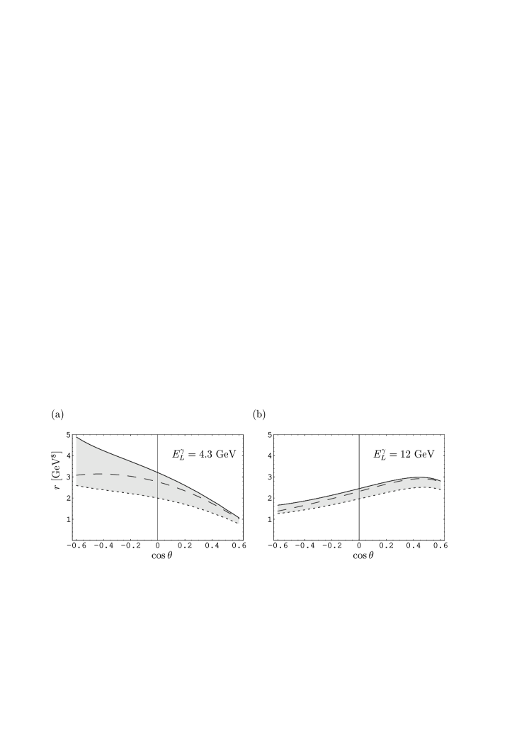
Figure 1: (a) The ratio $r$ defined in Eq. (6) at $E_{L}^{\gamma}=4.3\,{\rm GeV}$ for scenarios 1 (full), 2 (long-dashed), 3 (short-dashed). The form factors $R_{V}$ and $R_{A}$ are taken from the model in DFJK1 and $R_{T}$ is neglected. (b) The same for $E_{L}^{\gamma}=12\,{\rm GeV}$.

Numerical results for the Compton cross section evaluated from (Proton mass effects in wide-angle Compton scattering) without the $R_{T}$ and $\alpha_{s}$ corrections are shown in Fig. 1(a) for the three scenarios. We plot the ratio

$$r=t^{4}\frac{d\sigma/dt}{d\sigma_{\mathrm{KN}}/dt},$$ (6)

where

$$\frac{d\sigma_{\mathrm{KN}}}{dt}\ =\ \frac{2\pi\alpha_{\rm elm}^{2}}{(s-m^{2})^{2}}\;$$ (7)

$$\times\left[-\frac{s-m^{2}}{u-m^{2}}-\frac{u-m^{2}}{s-m^{2}}+\frac{4m^{2}t\,(m^{4}-su)}{(s-m^{2})^{2}(u-m^{2})^{2}}\right]$$

is the Klein-Nishina cross section for a point-like proton. The ratio $r$ essentially measures an average of $(t^{2}R_{V})^{2}$ and $(t^{2}R_{A})^{2}$. These scaled form factors are expected to depend only weakly on $t$ in the kinematical range considered here DFJK1 ; DFJK2 .

For a beam energy of $4.3\,{\rm GeV}$ the differences between the cross sections evaluated in the three scenarios are moderate at small scattering angles but grows up to a factor 2 for backward angles. With a beam energy of $12\,{\rm GeV}$ instead, the ambiguities are small for all angles considered, as shown in Fig. 1(b).

In DFJK1 ; DFJK2 ; hkm we plotted the scaled Compton cross section $s^{6}d\sigma/dt$ with the squared proton mass neglected in both the internal and external variables, i.e. we used scenario 3 together with $s=\hat{s}$, $t=\hat{t}$, $u=\hat{u}$ and replaced $(s-m^{2})^{2}$ with $s^{2}$ in (Proton mass effects in wide-angle Compton scattering). In this case the scattering angle $\theta$ and the scaling parameter $s^{6}$ multiplying the differential cross section do not correspond to the experimentally measured quantities. As a consequence both data and theoretical predictions in the plots of DFJK1 ; DFJK2 ; hkm were shifted. In other words we plotted $(2mE_{L}^{\gamma})^{6}d\sigma/dt$ against $1+t/(mE_{L}^{\gamma})$ rather than $s^{6}d\sigma/dt$ against $\cos\theta$. We realize that this is a rather confusing procedure which should be avoided in future presentations (we thank Travis Brooks and Lance Dixon for drawing our attention to this problem). Nevertheless, if our kinematical requirements of $s,-t,-u\gg\Lambda^{2}$ are well satisfied the expressions given in DFJK1 ; DFJK2 ; hkm are correct. The subtleties of internal vs. external Mandelstam variables matter only for energies as low as those currently available at JLAB, where the application of the handbag approach requires some care and is perhaps more qualitative.

Another interesting quantity is the correlation between the helicities of the incoming photon and the incoming ($A_{LL}$) or the outgoing ($K_{LL}$) proton in the c.m. In the handbag approach these parameters are given to leading $\mathcal{O}(\alpha_{s})$ by DFJK2 ; hkm

$$\frac{d\sigma}{dt}A_{LL}=\frac{d\sigma}{dt}K_{LL}=\frac{2\pi\alpha_{\rm elm}^{2}}{(s-m^{2})^{2}}$$ (8)

$$\times \frac{\hat{s}^{2}-\hat{u}^{2}}{|\hat{s}\hat{u}|}\,R_{A}(\hat{t})\,\Big{(}R_{V}(\hat{t})+\frac{\hat{t}}{\hat{s}+\sqrt{-\hat{s}\hat{u}}}\,R_{T}(\hat{t})\Big{)}.$$

The corresponding expressions for a point-like proton are

$$\frac{d\sigma^{\mathrm{KN}}}{dt}\,A_{LL}^{\mathrm{KN}}=\frac{2\pi\alpha_{\mathrm{em}}^{2}}{(s-m^{2})^{2}}\,$$ (9)

$$\quad\times\left[-\frac{s-m^{2}}{u-m^{2}}+\frac{u-m^{2}}{s-m^{2}}-\frac{2m^{2}t^{2}(s-u)}{(s-m^{2})^{2}\,(u-m^{2})^{2}}\right]\ ,$$

$$\frac{d\sigma^{\mathrm{KN}}}{dt}\,K_{LL}^{\mathrm{KN}}=\frac{2\pi\alpha_{\mathrm{em}}^{2}}{(s-m^{2})^{2}}\,$$

$$\quad\times\left[-\frac{s-m^{2}}{u-m^{2}}+\frac{u-m^{2}}{s-m^{2}}-\frac{4m^{2}t^{2}(m^{4}-su)}{(s-m^{2})^{3}\,(u-m^{2})^{2}}\right]\,,$$

which reduces to $A_{LL}^{\mathrm{KN}}=K_{LL}^{\mathrm{KN}}=(s^{2}-u^{2})/(s^{2}+u^{2})$ in the massless limit. In Fig. 2 we show the helicity correlation $K_{LL}$ evaluated for the three scenarios, normalized to the Klein-Nishina value. This quantity is essentially a measure of $R_{A}/R_{V}$, as can be seen from

$$\frac{K_{LL}}{K_{LL}^{\mathrm{KN}}}\simeq\frac{R_{A}}{R_{V}}\,\left[1-\frac{t^{2}}{2(s^{2}+u^{2})}\Big{(}1-\frac{R_{A}^{2}}{R_{V}^{2}}\Big{)}\right]^{-1},$$ (10)

where we have neglected $R_{T}$ and kinematic corrections of order $m^{2}/s$. Note that the kinematical prefactor in brackets is at most 0.3 for $\cos\theta\geq-0.6$ and $s\gg m^{2}$. Fig. 2 shows that for present JLAB energies the uncertainties related to the proton mass are sizeable, while at $E_{L}^{\gamma}=12$ GeV the effect is small.

JLAB will also measure the correlation $K_{LS}$ between the helicity of the incoming photon and the sideways polarization of the outgoing proton. In the handbag approach it is given by hkm

$$\frac{d\sigma}{dt}K_{LS}=\frac{2\pi\alpha_{\rm elm}^{2}}{(s-m^{2})^{2}}$$

$$\times \frac{\hat{s}^{2}-\hat{u}^{2}}{|\hat{s}\hat{u}|}\,\frac{\sqrt{-\hat{t}\,}}{2m}\,\Big{(}R_{T}(\hat{t})+\frac{4m^{2}}{\hat{s}+\sqrt{-\hat{s}\hat{u}}}\,R_{V}(\hat{t})\Big{)}\,R_{A}(\hat{t})$$

to leading $\mathcal{O}(\alpha_{s})$, with the sign convention detailed in hkm . Contrary to the previous observables, $K_{LS}$ is rather sensitive to the tensor Compton form factor $R_{T}$. It is convenient to consider the ratio $K_{LS}/K_{LL}$ where in the handbag approach the form factor $R_{A}$ drops out. Introducing the abbreviation

$$\kappa_{T}(\hat{t})\equiv\frac{\sqrt{-\hat{t}}}{2m}\,\frac{R_{T}(\hat{t})}{R_{V}(\hat{t})}\,,$$ (12)

this ratio can be expressed as hkm

$$\frac{K_{LS}}{K_{LL}}=\kappa_{T}\bigg{(}1+\frac{2m\sqrt{-\hat{t}}}{\hat{s}+\sqrt{-\hat{s}\hat{u}}}\,\frac{1}{\kappa_{T}}\bigg{)}\bigg{(}1-\frac{2m\sqrt{-\hat{t}}}{\hat{s}+\sqrt{-\hat{s}\hat{u}}}\,{\kappa_{T}}\bigg{)}^{-1}\!.$$ (13)

A rough estimate for the quantity $\kappa_{T}$ can be obtained by considering the analogy between the ratio $R_{T}/R_{V}$ and its electromagnetic counterpart $F_{2}/F_{1}$. One may, for instance, assume that

$$\kappa_{T}(\hat{t})\simeq\frac{\sqrt{-\hat{t}}}{2m}\,\frac{F_{2}(\hat{t})}{F_{1}(\hat{t})}\approx 0.37\,,$$ (14)

where the numerical value on the r.h.s. is taken from the measurement of $F_{2}/F_{1}$ for $-t=1\div 5.6\,{\rm GeV}^{2}$ Gayou:2001qd . (Note, however, that on the basis of the previous SLAC measurement of $F_{2}/F_{1}$ Andivahis:1994rq one would rather conclude that $\kappa_{T}\propto m/\sqrt{-t}$. For a detailed discussion of the uncertainties in the measurement of the Pauli form factor see Arrington:2002cr .) We use (14) to estimate $K_{LS}$ in the handbag approach and plot $K_{LS}/K_{LL}$ for the three scenarios in Fig. 3. We observe that the ratio $K_{LS}/K_{LL}$ is rather insensitive to the proton mass effects already at the present JLAB energy (in contrast, the predictions for $K_{LS}$ alone suffer from the same uncertainties as for the other Compton observables discussed above). Measuring the ratio $K_{LS}/K_{LL}$ at present JLAB energies, and solving for $\kappa_{T}(\hat{t})$ in (13) thus enables us to determine the ratio $R_{T}/R_{V}$ and to test the analogy with $F_{2}/F_{1}$ in (14).

In conclusion, we found that finite proton mass effects severely limit the quantitative test of the handbag approach and the extraction of the Compton form factors in wide angle Compton scattering for present JLAB energies. An exception is the ratio $K_{LS}/K_{LL}$ which turns out to be rather insensitive to finite proton mass effects, and can be used to determine the ratio of Compton form factors $R_{T}/R_{V}$. Qualitative features, like the sign and order of magnitude of the helicity correlations $K_{LL}$ or $K_{LS}$, are not affected either. For higher photon energies as projected for JLAB the theoretical uncertainties from the proton mass become reasonably small.

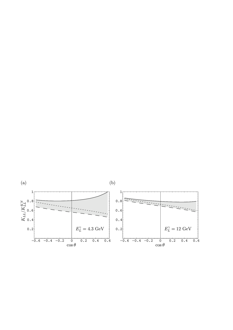
Figure 2: (a) The ratio $K_{LL}/K_{LL}^{\mathrm{KN}}$ of helicity correlations at $E_{L}^{\gamma}=4.3\,{\rm GeV}$ for scenarios 1 (full), 2 (long-dashed), 3 (short-dashed). $R_{V}$ and $R_{A}$ are taken from the model in DFJK1 and $R_{T}$ is neglected. (b) The same for $E_{L}^{\gamma}=12\,{\rm GeV}$.

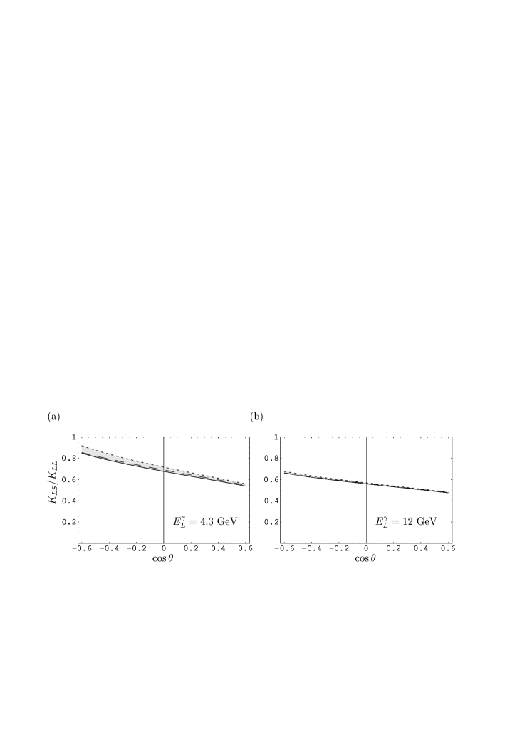
Figure 3: (a) The ratio $K_{LS}/K_{LL}$ of helicity correlations at $E_{L}^{\gamma}=4.3\,{\rm GeV}$ for scenarios 1 (full), 2 (long-dashed), 3 (short-dashed). $R_{V}$ is taken from the model in DFJK1 and $R_{T}$ is estimated from (14). (b) The same for $E_{L}^{\gamma}=12\,{\rm GeV}$.

References

(1) M. Diehl, T. Feldmann, R. Jakob and P. Kroll,
Eur. Phys. J. C 8, 409 (1999)
[hep-ph/9811253].
(2) M. Diehl, T. Feldmann, R. Jakob and P. Kroll,
Phys. Lett. B 460, 204 (1999)
[hep-ph/9903268].
(3) H. W. Huang, P. Kroll and T. Morii,
Eur. Phys. J. C 23, 301 (2002)
[hep-ph/0110208].
(4) A. V. Radyushkin,
Phys. Rev. D 58, 114008 (1998)
[hep-ph/9803316].
(5)
J. P. Chen et al. [Jefferson Lab Hall A Collaboration],
“Exclusive Compton Scattering On The Proton,”
Jefferson Lab preprint PCCF-RI-99-17.
(6)
O. Gayou et al. [Jefferson Lab Hall A Collaboration],
Phys. Rev. Lett. 88, 092301 (2002)
[nucl-ex/0111010].
(7)
L. Andivahis et al.,
Phys. Rev. D 50, 5491 (1994).
(8)
J. Arrington,
hep-ph/0209243.