Two–loop corrections to Radiative Electroweak

Symmetry Breaking in the MSSM

Abstract

We study the ${\cal O}(\alpha_{t}\alpha_{s}+\alpha_{t}^{2})$ two–loop corrections to the minimization conditions of the MSSM effective potential, providing compact analytical formulae for the Higgs tadpoles. We connect these results with the renormalization group running of the MSSM parameters from the grand unification scale down to the weak scale, and discuss the corrections to the Higgs mixing parameter $\mu$ and to the running CP–odd Higgs mass $m_{\scriptscriptstyle A}$ in various scenarios of gravity–mediated SUSY breaking. We find that the ${\cal O}(\alpha_{t}\alpha_{s})$ and ${\cal O}(\alpha_{t}^{2})$ contributions partially cancel each other in the minimization conditions. In comparison with the full one–loop corrections, the ${\cal O}(\alpha_{t}\alpha_{s}+\alpha_{t}^{2})$ two–loop corrections significantly weaken the dependence of the parameters $\mu$ and $m_{\scriptscriptstyle A}$ on the renormalization scale at which the effective potential is minimized. The residual two–loop and higher–order corrections to $\mu$ and $m_{\scriptscriptstyle A}$ are estimated to be at most 1% in the considered scenarios.

1 Introduction

One of the most attractive features of the Minimal Supersymmetric extension of the Standard Model (MSSM) [1], is the fact that it provides a mechanism for breaking radiatively the electroweak gauge $SU(2)_{L}\times U(1)_{Y}$ symmetry down to $U(1)_{\rm EM}$. It was first shown [2] that a supersymmetry (SUSY) breaking term for the gluino can induce an effective potential which spontaneously breaks the electroweak symmetry. At the same time, a mechanism relying on the renormalization group evolution from a grand unification (GUT) scale $M_{\scriptscriptstyle GUT}$ down to the weak scale was proposed [3]. In this framework, at the scale $M_{\scriptscriptstyle GUT}$, the parameters entering the scalar potential of the MSSM obey simple boundary conditions dictated by the underlying theory of SUSY breaking, and the electroweak symmetry is unbroken. When the parameters are evolved down to the weak scale by means of the MSSM renormalization group equations (RGE), which amounts to resumming the leading logarithmic corrections to all orders, the soft SUSY–breaking mass $m^{2}_{H_{2}}$ is driven towards negative values, due to corrections controlled by the top Yukawa coupling $h_{t}$. This helps to destabilize the origin in field space, so that the Higgs fields acquire non–vanishing vacuum expectation values (VEVs) and the electroweak symmetry is spontaneously broken. Although the studies in Refs. [2, 3] where differing on the initial boundary conditions, the result was one: the radiative electroweak symmetry breaking (REWSB) takes place if the top Yukawa coupling is large, such that $60\;{\rm GeV}\lower 3.01385pt\hbox{$\;\stackrel{{\scriptstyle\textstyle<}}{{\sim}}\;$}m_{t}\lower 3.01385pt\hbox{$\;\stackrel{{\scriptstyle\textstyle<}}{{\sim}}\;$}200\;{\rm GeV}$, with the upper bound coming from the requirement that $h_{t}$ remains in the perturbative range up to the GUT scale. It could be a coincidence that the top quark is found at the Tevatron to have mass around 175 GeV, but certainly this is consistent with the REWSB mechanism in the MSSM.

In the RGE–improved potential of the MSSM employed at tree level, the VEVs of the Higgs fields, and the occurrence of spontaneous symmetry breaking itself, depend critically on the renormalization scale at which the parameters entering the potential are computed; an inappropriate choice of that scale can lead to results that are even qualitatively wrong. In fact, the electroweak symmetry is either broken or unbroken, independently of the renormalization scale choice, and the critical behavior described above is just an artifact of the tree–level approximation. The correct way of determining the ground state of the theory is to minimize the Coleman–Weinberg effective potential [4], i.e. the tree–level potential plus a correction coming from the sum of all the one–loop diagrams with zero–momentum external lines. Since Refs. [5, 6] this procedure has become standard in the renormalization group analyses of the MSSM (for early examples see Refs. [7, 8]).

The effective potential is also a useful tool for computing the leading corrections to the MSSM Higgs masses, both at the one loop [9] and the two loop [10, 11, 12, 13, 14] level, in the approximation of zero external momentum. The leading one–loop corrections are ${\cal O}(\alpha_{t})$, i.e. they are controlled by the top Yukawa coupling $h_{t}\equiv\sqrt{4\pi\alpha_{t}}$. For stop masses of ${\cal O}(1\,{\rm TeV})$, such corrections increase by 40–60 GeV the mass $m_{h}$ of the lightest Higgs boson (which at tree level must be lighter than $m_{\scriptscriptstyle Z}$), allowing it to escape the direct searches at LEP. Also, the leading two–loop corrections have sizeable effects: the ${\cal O}(\alpha_{t}\alpha_{s})$ corrections, controlled by the strong gauge coupling $g_{s}\equiv\sqrt{4\pi\alpha_{s}}\,$, typically reduce $m_{h}$ by 15–20 GeV, whereas the ${\cal O}(\alpha_{t}^{2})$ ones may increase it by up to 7–8 GeV.

Motivated by the relevance of the ${\cal O}(\alpha_{t}\alpha_{s}+\alpha_{t}^{2})$ two–loop corrections in the case of the Higgs masses, we study in this paper the effect of the same corrections on the electroweak symmetry breaking conditions. The contributions to the two–loop MSSM effective potential that are relevant to the ${\cal O}(\alpha_{t}\alpha_{s}+\alpha_{t}^{2})$ corrections have been discussed in Refs. [10, 11, 12], and a complete computation of the two–loop effective potential has been presented in Ref. [17]. However, practical studies of REWSB usually require explicit formulae for the Higgs tadpole diagrams, i.e. the first derivatives of the effective potential with respect to the Higgs fields. Such formulae are presently available at the one–loop order [7], but they have not been presented so far at the two–loop order. Using the techniques developed in Ref. [12], we compute in this paper explicit and compact analytical expressions for the two–loop ${\cal O}(\alpha_{t}\alpha_{s}+\alpha_{t}^{2})$ part of the tadpoles. As a byproduct from our ${\cal O}(\alpha_{t}\alpha_{s})$ corrections we obtain also the ${\cal O}(\alpha_{b}\alpha_{s})$ corrections, that are relevant for large values of $\tan\beta$. Once we assume that the electroweak symmetry is indeed broken, giving rise to the observed value of the $Z$ boson mass, the corrections to the tadpoles translate into ${\cal O}(\alpha_{t}\alpha_{s}+\alpha_{t}^{2})$ corrections to the values of $\mu$, the Higgs mass term in the superpotential, and $m_{\scriptscriptstyle A}$, the running mass of the $A$ boson. We discuss the effect of our two–loop corrections in the framework of gravity mediated SUSY breaking [18], also denoted as minimal supergravity (mSUGRA), referring in particular to various “benchmark” scenarios suggested at Snowmass [19]. We find that the inclusion of the ${\cal O}(\alpha_{t}\alpha_{s}+\alpha_{t}^{2})$ corrections significantly improves the renormalization scale dependence of the results, and that partial cancellations occur between the ${\cal O}(\alpha_{t}\alpha_{s})$ corrections and the ${\cal O}(\alpha_{t}^{2})$ ones. Our corrections are also required for consistency in the ${\cal O}(\alpha_{t}\alpha_{s}+\alpha_{t}^{2})$ two–loop computation of the MSSM Higgs masses, if the input parameters are computed via renormalization group evolution from a set of high energy boundary conditions.

The paper is organized as follows: in section 2 we recall the basic concepts of radiative electroweak symmetry breaking, and introduce some notation which will be used in the rest of the paper; in section 3 we describe the main features of our ${\cal O}(\alpha_{t}\alpha_{s}+\alpha_{t}^{2})$ computation of the two–loop tadpoles; in section 4 we discuss the numerical effect of our corrections, and we show how they improve the dependence of $\mu$ and $m_{\scriptscriptstyle A}$ on the renormalization scale at which the effective potential is minimized; section 5 contains our conclusions. In addition, we present in the appendix A some useful formulae for the integrals entering the two–loop effective potential, and in the appendix B the explicit analytical formulae for the ${\cal O}(\alpha_{t}\alpha_{s})$ part of the corrections. The formulae for the ${\cal O}(\alpha_{t}^{2})$ part are indeed rather long, thus we make them available, upon request, in the form of a computer code .

2 Radiative electroweak symmetry breaking

We start our discussion from the tree–level scalar potential of the MSSM, that reads, keeping only the dependence on the neutral Higgs fields $H_{1}^{0}$ and $H_{2}^{0}$:

$$V_{0}=\Lambda+m_{1}^{2}\,\left|H_{1}^{0}\right|^{2}+m_{2}^{2}\,\left|H_{2}^{0}\right|^{2}+m_{3}^{2}\,\left(H_{1}^{0}H_{2}^{0}+{\rm h.c.}\right)+{g^{2}+g^{\prime\,2}\over 8}\left(|H_{1}^{0}|^{2}-|H_{2}^{0}|^{2}\right)^{2}\,,$$ (1)

where: $\Lambda$ is a field–independent vacuum energy; $m_{1}^{2}=m_{H_{1}}^{2}+\mu^{2}$, $\,m_{2}^{2}=m_{H_{2}}^{2}+\mu^{2}$ (we assume $\mu$ to be real, neglecting all possible CP–violating phases); $m_{H_{1}}^{2}$, $m_{H_{2}}^{2}$ and $m_{3}^{2}$ are soft SUSY–breaking masses; $g$ and $g^{\prime}$ are the $SU(2)_{L}$ and $U(1)_{Y}$ gauge couplings, respectively. At the classical level, the mass parameters entering $V_{0}$ must satisfy the following conditions:

$$m_{1}^{2}+m_{2}^{2}\;\geq\;2\,|m_{3}^{2}|\;\;,\hskip 56.9055ptm_{1}^{2}\,m_{2}^{2}\;\leq\;m_{3}^{4}\,.$$ (2)

The first condition guarantees that the potential is bounded from below; the second condition destabilizes the origin in field space, making sure that the neutral components of the Higgs fields acquire non–vanishing VEVs $\langle H_{1}^{0}\rangle\equiv v_{1}/\sqrt{2}$ and $\langle H_{2}^{0}\rangle\equiv v_{2}/\sqrt{2}$. It is not restrictive to choose $m_{3}^{2}$ real and negative, so that $v_{1}$ and $v_{2}$ are real and positive, and the neutral Higgs fields can be decomposed into their VEVs plus their CP–even and CP–odd fluctuations as $H_{i}^{0}=(v_{i}+S_{i}+iP_{i})/\sqrt{2}$.

Since the parameters entering $V_{0}$ are taken as ”running” ones (i.e., they vary with the renormalization scale), also the validity of the conditions in Eq. (2) depends on the scale, as well as the numerical values of $v_{1}$ and $v_{2}$. As discussed in Ref. [6], the minimization of the tree–level potential may lead to grossly inaccurate results, unless the renormalization scale is chosen in such a way that the radiative corrections to the scalar potential are small. To obtain the correct results, one should rather minimize the effective potential $V_{\rm eff}$, defined as:

$$V_{\rm eff}=V_{0}+\Delta V\,,$$ (3)

where $\Delta V$ contains the radiative corrections to the scalar potential $V_{0}$. The minimization conditions for $V_{\rm eff}$ can be written as:

$$\frac{1}{v_{1}}\left.\frac{\partial V_{\rm eff}}{\partial S_{1}}\right|_{\rm min} = m^{2}_{H_{1}}+\mu^{2}+\frac{g^{2}+g^{\prime\,2}}{4}\,(v_{1}^{2}-v_{2}^{2})+m_{3}^{2}\,\frac{v_{2}}{v_{1}}+\Sigma_{1}\;\;\;=\;0\,,$$ (4)

$$\frac{1}{v_{2}}\left.\frac{\partial V_{\rm eff}}{\partial S_{2}}\right|_{\rm min} = m^{2}_{H_{2}}+\mu^{2}+\frac{g^{2}+g^{\prime\,2}}{4}\,(v_{2}^{2}-v_{1}^{2})+m_{3}^{2}\,\frac{v_{1}}{v_{2}}+\Sigma_{2}\;\;\;=\;0\,,$$ (5)

where the “tadpoles” $\Sigma_{1}$ and $\Sigma_{2}$ are defined as:

$$\Sigma_{i}\equiv\frac{1}{v_{i}}\left.\frac{\partial\Delta V}{\partial S_{i}}\right|_{\rm min}\,.$$ (6)

In principle, a renormalization group study of the MSSM should start from some large scale $M_{\scriptscriptstyle GUT}$, where the input parameters have a simple structure dictated by the underlying theory of SUSY breaking, and the electroweak symmetry is unbroken. The parameters are then evolved, by means of appropriate renormalization group equations, down to some lower scale, where the electroweak symmetry breaking occurs and the VEVs $v_{1}$ and $v_{2}$ can be obtained by solving Eqs. (4)–(5). A set of high–energy input parameters is then acceptable if it leads to the correct value of the squared running mass for the $Z$ boson, $m_{\scriptscriptstyle Z}^{2}=(g^{2}+g^{\prime\,2})\,(v_{1}^{2}+v_{2}^{2})/4$. However, in most practical applications of the renormalization group procedure, it is more convenient to assume that there is successful electroweak symmetry breaking, and trade two of the high–energy input parameters for $v_{1}$ and $v_{2}$ (or, equivalently, for $v^{2}\equiv v_{1}^{2}+v_{2}^{2}$ and $\tan\beta\equiv v_{2}/v_{1}$). Eqs. (4)–(5) can thus be rephrased into the following conditions among the parameters at the weak scale:

$$\mu^{2} = -\frac{m_{\scriptscriptstyle Z}^{2}}{2}+\frac{m^{2}_{H_{1}}+\Sigma_{1}-(m^{2}_{H_{2}}+\Sigma_{2})\,\tan^{2}\beta}{\tan^{2}\beta-1}\,,$$ (7)

$$m_{3}^{2} = -\frac{1}{2}\,\sin 2\beta\,\left(m^{2}_{H_{1}}+m^{2}_{H_{2}}+2\,\mu^{2}+\Sigma_{1}+\Sigma_{2}\right)\,,$$ (8)

i.e., the terms proportional to $\Sigma_{1}$ and $\Sigma_{2}$ in the above equations can be viewed as the radiative corrections to the values of $\mu^{2}$ and $m_{3}^{2}$ obtained from the requirement of successful electroweak symmetry breaking. We recall that $m_{3}^{2}$ is related to the squared running mass for the $A$ boson through $m_{\scriptscriptstyle A}^{2}=-2\,m_{3}^{2}/\sin 2\beta$. Notice also that the sign of $\mu$ is not fixed by Eq. (7), and it must be supplemented as an additional input quantity. If the right side of Eq. (7) is such that $\mu^{2}$ is negative, then our choice of input parameters is inconsistent, and the electroweak symmetry fails to be broken. We remark in passing that the choice of the input parameters is constrained by further requirements: it must lead to a spectrum of physical masses for the MSSM superpartners and Higgs bosons compatible with the present experimental lower bounds, and such that the lightest supersymmetric particle (LSP) is electrically neutral; it must satisfy phenomenological constraints coming from radiative B-meson decays, muon anomalous magnetic moment and cosmological relic density; finally, it must guarantee that the MSSM scalar potential is bounded from below and does not lead to charge and color breaking minima. However, a detailed study of the (theoretically and experimentally) allowed regions in the MSSM parameter space goes beyond the scope of this paper, and will not be pursued in the following.

The full one–loop corrections to the REWSB conditions have been extensively discussed in the literature [7] in the framework of the mSUGRA scenario. The dominant one–loop contributions to $\Sigma_{1}$ and $\Sigma_{2}$ come to a large extent from the top/stop (and, for large $\tan\beta$, bottom/sbottom and tau/stau) diagrams. The contributions of the diagrams involving charginos and neutralinos can also be sizeable and comparable to the top/stop ones in some regions of the parameter space, while the Higgs and gauge bosons and the first two generations of (s)quarks and (s)leptons give only subdominant corrections.

In the following sections we provide explicit analytical formulae for the two–loop top/stop contributions to the tadpoles $\Sigma_{1}$ and $\Sigma_{2}$, resulting into ${\cal O}(\alpha_{t}\alpha_{s}+\alpha_{t}^{2})$ corrections to $\mu^{2}$ and to the running mass $m_{\scriptscriptstyle A}^{2}$. In analogy with the case of the Higgs masses, we expect such corrections to be the leading ones at the two–loop level, giving rise to sizeable effects at least in some regions of the MSSM parameter space. In addition, most public codes that compute the MSSM mass spectrum from a set of unified parameters at the scale $M_{\scriptscriptstyle GUT}$, such as SuSpect [20], SoftSusy [21], SPheno [22] and FeynSSG [23], include a two–loop ${\cal O}(\alpha_{t}\alpha_{s}+\alpha_{t}^{2})$ computation of the Higgs masses, but employ one–loop results for the tadpoles (see also Ref. [25] for a recent discussion). Since $m_{\scriptscriptstyle A}^{2}$ enters the tree–level mass matrix of the CP–even Higgs bosons, the ${\cal O}(\alpha_{t}\alpha_{s}+\alpha_{t}^{2})$ corrections to $m_{\scriptscriptstyle A}^{2}$ should be included in those codes for consistency.

3 Computation of the ${\cal O}(\alpha_{t}\alpha_{s}+\alpha_{t}^{2})$ corrections

We shall now describe our two–loop, ${\cal O}(\alpha_{t}\alpha_{s}+\alpha_{t}^{2})$ computation of the tadpoles $\Sigma_{1}$ and $\Sigma_{2}$, involving the first derivatives of $\Delta V$ with respect to the CP–even parts of the neutral Higgs fields [see Eq. (6)]. The computation is consistently performed by setting to zero all the gauge couplings but $g_{s}$ and by keeping $h_{t}$ as the only non–vanishing Yukawa coupling (with a slight abuse of language, in the following we will refer to this approximation as to the gaugeless limit). In this limit, the tree–level (field–dependent) spectrum of the MSSM simplifies considerably: gauginos and Higgsinos do not mix; the charged and neutral Higgsinos combine into Dirac spinors $\tilde{h}^{0}$ and $\tilde{h}^{\pm}$ with degenerate mass $\mu$; the gaugino masses coincide with the soft SUSY–breaking parameters $M_{A}\;(A=1,2,3)\;$ (among them, only the gluino mass $m_{\tilde{g}}=M_{3}$ is relevant to our calculation); the only massive Standard Model (SM) fermion is the top quark; all other fermions and gauge bosons have vanishing masses; besides the top squarks, the only sfermion with non–vanishing couplings is the bottom squark $\tilde{b}_{L}$; the lighter CP–even Higgs boson, $h$, is massless, and the same is true for the Goldstone bosons $G$ and $G^{\pm}$; all the remaining Higgs states, $(H,A,H^{\pm})$, have degenerate mass eigenvalues $m_{\scriptscriptstyle A}^{2}$. The tree–level mixing angle in the CP–even sector is just $\alpha=\beta-\pi/2$.

To begin with, we address the renormalization of the effective potential. In the loop expansion, the correction to the effective potential can be decomposed as $\Delta V=V_{1\ell}+V_{2\ell}+\cdots$, where the ellipsis stand for higher loops. Using the Landau gauge and dimensional reduction [26, 27] in $d=4-2\epsilon$ dimensions, and including for later convenience also terms that vanish when $\epsilon\rightarrow 0$, the unrenormalized one–loop effective potential reads:

$$V_{1\ell}=\frac{-1\;\;\;}{64\pi^{2}}\,{\rm Str}\;{\cal M}^{4}\left[\frac{1}{\epsilon}+\frac{3}{2}-\ln\frac{{\cal M}^{2}}{Q^{2}}+\epsilon\,\left(\frac{7}{4}-\frac{3}{2}\,\ln\frac{{\cal M}^{2}}{Q^{2}}+\frac{1}{2}\ln^{2}\frac{{\cal M}^{2}}{Q^{2}}+\frac{\,\pi^{2}}{12}\right)\,\right]\,,$$ (9)

where ${\cal M}^{2}$ is the matrix of the field–dependent squared masses, and the supertrace of a generic function $f({\cal M}^{2})$ is defined as a sum over the eigenvalues $m^{2}_{i}$:

$${\rm Str}\,f({\cal M}^{2})=\sum_{i}(-1)^{2s_{i}}(2s_{i}+1)\,f(m^{2}_{i})\;,$$ (10)

where $s_{i}$ is the spin of the corresponding particles. In Eq. (9), $Q^{2}=4\pi\mu^{2}e^{-\gamma_{E}}$, i.e. the finite terms that are removed together with $1/\epsilon$ in the modified subtraction schemes have been reabsorbed in the renormalization scale (the same convention will be adopted in the following). In the gaugeless limit described above, only the top and stop contributions to $V_{1\ell}$ are relevant, giving rise to ${\cal O}(\alpha_{t})$ contributions to $\Sigma_{1}$ and $\Sigma_{2}$.

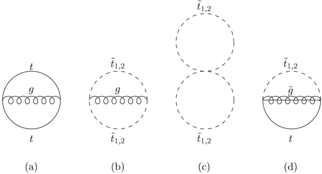
Figure 1: Feynman diagrams that contribute to the two–loop effective potential and affect the ${\cal O}(\alpha_{t}\alpha_{s})$ corrections to the electroweak symmetry breaking conditions. The diagrams relevant to the ${\cal O}(\alpha_{b}\alpha_{s})$ corrections can be obtained with the replacement $t\to b$.

The Feynman diagrams that contribute to the two–loop effective potential $V_{2\ell}$ and give rise to ${\cal O}(\alpha_{t}\alpha_{s})$ contributions to $\Sigma_{1}$ and $\Sigma_{2}$ are shown in Fig. 1, while the diagrams relevant to the ${\cal O}(\alpha_{t}^{2})$ contributions are shown in Fig. 2. The corresponding analytical formulae for $V_{2\ell}$ can be found e.g. in the last paper of Ref. [11] . These formulae involve two basic integrals, $I(m_{1}^{2},m_{2}^{2},m_{3}^{2})$ and $J(m_{1}^{2},m_{2}^{2})$, that have been evaluated with different methods in Refs. [28, 29]. Explicit expressions for $I$ and $J$ in the formalism of Ref. [29] are presented in the appendix A.

To carry out the renormalization of $V_{\rm eff}$, at the two–loop order and in the $\overline{\rm DR}$ scheme [26, 27], we start from the unrenormalized effective potential, written in terms of generic bare parameters $x_{i}$. Then, we expand the parameters as $x_{i}=x_{i}^{\overline{\rm\scriptscriptstyle DR}}+\delta x_{i}$, where $\delta x_{i}$ are purely divergent quantities, so that all the poles in $1/\epsilon$ and $1/\epsilon^{2}$ are cancelled. After taking the limit $\epsilon\rightarrow 0$, the non vanishing part of the renormalized effective potential is:

$$V_{\rm eff}=V_{0}(x^{\overline{\rm\scriptscriptstyle DR}}_{i})+V^{(1)}_{1\ell}(x^{\overline{\rm\scriptscriptstyle DR}}_{i})+V_{2\ell}^{(1)}+\frac{\partial V_{1\ell}^{(\epsilon)}}{\partial x_{i}}\,\delta^{1\ell}x_{i}\,,$$ (11)

where $V_{1\ell}^{(1)}$ and $V_{2\ell}^{(1)}$ denote the finite parts of the one–loop and two–loop effective potential, respectively, $V_{1\ell}^{(\epsilon)}$ denotes the terms proportional to $\epsilon$ in Eq. (9), and $\delta^{1\ell}x_{i}$ is the coefficient of $1/\epsilon$ in the one–loop part of the generic counterterm (notice that we need to compute explicitly only the one–loop counterterms for the top and stop masses). In Eq. (11), $V_{0}$ and $V_{1\ell}^{(1)}$ are expressed in terms of $\overline{\rm DR}$–renormalized parameters, while the renormalization of the parameters entering the two–loop part is irrelevant, amounting to a higher–order (i.e., three–loop) effect. In summary, it is possible to define the renormalized two–loop effective potential as:

$$\widehat{V}_{2\ell}=V_{2\ell}^{(1)}+\frac{\partial V_{1\ell}^{(\epsilon)}}{\partial x_{i}}\,\delta^{1\ell}x_{i}\,.$$ (12)

We have checked that $\widehat{V}_{2\ell}$ corresponds to the finite part of the potential obtained by replacing the integrals $I$ and $J$ in $V_{2\ell}$ with the “subtracted” integrals $\hat{I}$ and $\hat{J}$, first introduced in Ref. [28]. More precisely, this is true only up to terms that give a null contribution to $\Sigma_{1}$ and $\Sigma_{2}$, unless we include in $V_{\rm eff}$ also diagrams that do not depend on the Higgs fields (such as, e.g., the one–loop diagram involving gluinos and the two–loop diagram involving gluinos and gluons).

Compact analytical formulae for the derivatives of the renormalized effective potential in the gaugeless limit can be obtained with a procedure similar to that of Ref. [12]. The relevant field–dependent quantities are the top mass $m_{t}$, the stop masses $m_{\tilde{t}_{1}}^{2}$ and $m_{\tilde{t}_{2}}^{2}$, and the stop mixing angle $\theta_{\tilde{t}}\,$ (the top and stop phases $\varphi$ and $\widetilde{\varphi}$, introduced in [12] to take into account the dependence on the CP–odd part of the Higgs fields, do not enter the computation of $\Sigma_{1}$ and $\Sigma_{2}$). At the minimum of the effective potential, the parameters in the stop sector are related by:

$$\sin 2\theta_{\tilde{t}}=\frac{2\,m_{t}\,(A_{t}+\mu\,\cot\beta)}{m_{\tilde{t}_{1}}^{2}-m_{\tilde{t}_{2}}^{2}}\,,$$ (13)

where $A_{t}$ is the soft SUSY–breaking trilinear coupling of the stops [notice that Eq. (13) defines our convention for the sign of $\mu\,$]. We will use in the following the shortcuts $c_{2\theta}\equiv\cos 2\theta_{\tilde{t}}$ and $s_{2\theta}\equiv\sin 2\theta_{\tilde{t}}\,$. After a straightforward application of the chain rule for the derivatives of the effective potential, we get:

$$v_{1}^{2}\,\Sigma_{1} = m_{t}\,\mu\,\cot\beta\,s_{2\theta}\,F\,,$$ (14)

$$v_{2}^{2}\,\Sigma_{2} = m_{t}\,A_{t}\,s_{2\theta}\,F+2\,m_{t}^{2}\,G\,.$$ (15)

The functions $F$ and $G$ are combinations of the derivatives of $\Delta V$ with respect to the field–dependent parameters, computed at the minimum of the effective potential:

$$F = \frac{\partial\Delta V}{\partial m_{\tilde{t}_{1}}^{2}}-\frac{\partial\Delta V}{\partial m_{\tilde{t}_{2}}^{2}}-\frac{2\,c_{2\theta}}{m_{\tilde{t}_{1}}^{2}-m_{\tilde{t}_{2}}^{2}}\,\frac{\partial\Delta V}{\partial c_{2\theta}}\,,$$ (16)

$$G = \frac{\partial\Delta V}{\partial m_{t}^{2}}+\frac{\partial\Delta V}{\partial m_{\tilde{t}_{1}}^{2}}+\frac{\partial\Delta V}{\partial m_{\tilde{t}_{2}}^{2}}\,.$$ (17)

The one–loop parts of $F$ and $G$, giving rise to ${\cal O}(\alpha_{t})$ contributions to $\Sigma_{1}$ and $\Sigma_{2}$, are easily computed from the derivatives of $V_{1\ell}^{(1)}$. In units of $N_{c}/(16\,\pi^{2})$, where $N_{c}=3$ is a color factor, they read:

$$F^{1\ell} = m_{\tilde{t}_{1}}^{2}\left(\ln\frac{m_{\tilde{t}_{1}}^{2}}{Q^{2}}-1\right)-m_{\tilde{t}_{2}}^{2}\left(\ln\frac{m_{\tilde{t}_{2}}^{2}}{Q^{2}}-1\right)\,,$$ (18)

$$G^{1\ell} = m_{\tilde{t}_{1}}^{2}\left(\ln\frac{m_{\tilde{t}_{1}}^{2}}{Q^{2}}-1\right)+m_{\tilde{t}_{2}}^{2}\left(\ln\frac{m_{\tilde{t}_{2}}^{2}}{Q^{2}}-1\right)-2\,m_{t}^{2}\left(\ln\frac{m_{t}^{2}}{Q^{2}}-1\right)\,.$$ (19)

Although a naive, brute–force computation of the derivatives of the renormalized two–loop potential $\widehat{V}_{2\ell}$ presents no major conceptual difficulties, the number of terms involved blows up quickly, giving rise to very long and complicated analytical expressions. However, in the spirit of Ref. [29], it is possible to obtain recursive relations for the derivatives of the integral $I(m_{1}^{2},m_{2}^{2},m_{3}^{2})$ with respect to the internal masses (see the appendix A), that simplify considerably the results. In this way, we obtained compact analytical formulae for the two–loop parts of $F$ and $G$, giving rise to ${\cal O}(\alpha_{t}\alpha_{s}+\alpha_{t}^{2})$ contributions to $\Sigma_{1}$ and $\Sigma_{2}$. As a non trivial check of the correctness of our computation, we have verified that the quantities $\mu^{2}$ and $m_{3}^{2}$ defined in Eqs. (7)–(8) obey the appropriate two–loop RGE [30], specialized to the gaugeless limit:

$$\frac{\partial\mu^{2}}{\partial\ln Q^{2}} = \frac{3\,\alpha_{t}}{4\,\pi}\,\mu^{2}+\frac{\alpha_{t}\,\alpha_{s}}{\pi^{2}}\,\mu^{2}-\frac{9\,\alpha_{t}^{2}}{16\,\pi^{2}}\,\mu^{2}\,,$$ (20)

$$\frac{\partial m_{3}^{2}}{\partial\ln Q^{2}} = \frac{3\,\alpha_{t}}{4\,\pi}\left(\frac{m_{3}^{2}}{2}+A_{t}\,\mu\right)+\frac{\alpha_{t}\,\alpha_{s}}{\pi^{2}}\left(\frac{m_{3}^{2}}{2}+A_{t}\,\mu-m_{\tilde{g}}\,\mu\right)-\frac{9\,\alpha_{t}^{2}}{16\,\pi^{2}}\left(\frac{m_{3}^{2}}{2}+2\,A_{t}\,\mu\right)\,.$$

We have also checked explicitly that, in the special supersymmetric limit in which all the soft–SUSY breaking parameters as well as $\mu$ are set to zero, such that $m_{\tilde{t}_{1}}=m_{\tilde{t}_{2}}=m_{t}$, the two–loop parts of $F$ and $G$ are indeed vanishing.

For illustrative purposes, we present in the appendix B the explicit formulae for the ${\cal O}(\alpha_{t}\alpha_{s})$ corrections, valid for arbitrary values of the relevant MSSM parameters. The corresponding formulae for the ${\cal O}(\alpha_{t}^{2})$ corrections are indeed rather long, thus we make them available, upon request, in the form of a Fortran code.

The computation described above allows us to obtain also the two–loop ${\cal O}(\alpha_{b}\alpha_{s})$ corrections  induced by the bottom/sbottom sector ($h_{b}\equiv\sqrt{4\pi\alpha_{b}}$ being the bottom Yukawa coupling), that can be relevant for large values of $\tan\beta$. To this purpose, the substitutions $t\rightarrow b\,,\;v_{1}\leftrightarrow v_{2}$ (i.e., $\tan\beta\leftrightarrow\cot\beta$) and $\Sigma_{1}\leftrightarrow\Sigma_{2}$ must be performed in the corresponding formulae for the ${\cal O}(\alpha_{t}\alpha_{s})$ part of the corrections. The complications relative to the on–shell definition of the sbottom parameters, discussed in Ref. [13], do not arise in this case since we are working in the $\overline{\rm DR}$ renormalization scheme. However, the $\tan\beta$–enhanced threshold corrections [31] to the relation between $h_{b}$ and the bottom mass $m_{b}$ must be resummed to all orders [32] in a redefinition of the bottom Yukawa coupling (see e.g. Ref. [13] for the details).

4 Numerical results

In this section we discuss the numerical effect of our ${\cal O}(\alpha_{t}\alpha_{s}+\alpha_{t}^{2})$ two–loop corrections on the minimization conditions of the MSSM effective potential.

For definiteness, we work in the mSUGRA scenario, in which the MSSM Lagrangian at the large scale $M_{\scriptscriptstyle GUT}$ contains only five independent mass parameters: a common soft SUSY-breaking scalar mass $m_{0}$, a common soft gaugino mass $m_{1/2}$, a common soft trilinear term $A_{0}$, the superpotential Higgs mixing parameter $\mu_{0}$ and its soft SUSY-breaking counterpart $B_{0}$ (the subscript “0” denotes the fact that the parameters are computed at the boundary scale). The soft Higgs mixing parameter $B$ has the dimensions of a squared mass, and is defined in such a way that in the low–energy Higgs potential of Eq. (1) it coincides with $m_{3}^{2}$ (to avoid confusion, we will refer to $B$ as to $m_{3}^{2}\,$ from now on). As anticipated in section 2, rather than providing input values for all the five mass parameters at the GUT scale, we assume that the electroweak symmetry is successfully broken at the weak scale, and we trade $\mu_{0}$ and $m_{3}^{2}(M_{\scriptscriptstyle GUT})$ for the weak scale input parameters $v$ and $\tan\beta$.

Before discussing our results, it is useful to describe in some detail the numerical procedure for the renormalization group evolution of the MSSM parameters. We start by defining the $SU(3)\times SU(2)_{L}\times U(1)_{Y}$ gauge couplings at the weak scale (which we identify with the pole $Z$ boson mass, $M_{\scriptscriptstyle Z}=91.187$ GeV), from the running weak mixing angle $\hat{s}^{\,2}=0.2315$, the electromagnetic coupling $\widehat{\alpha}_{\scriptscriptstyle EM}=1/127.9$ and the strong coupling $\alpha_{s}=0.119$. The electroweak symmetry breaking parameter, $v^{2}=v_{1}^{2}+v_{2}^{2}\,$, is defined in terms the muon decay constant according to the relation $v=(\sqrt{2}\,G_{\mu})^{-1/2}=246.218$ GeV, and then translated to the $\overline{\rm DR}$ scheme by means of the formulae of Ref. [12]. In addition, $\tan\beta=v_{2}/v_{1}$ is taken as an input parameter at the weak scale, allowing us to determine $v_{1}$ and $v_{2}$. The Yukawa couplings of the light SM fermions are obtained from the corresponding masses at the scale $Q=2$ GeV, and then evolved up to $M_{\scriptscriptstyle Z}$ by means of the two–loop SM RGEs [33]. In the case of the bottom coupling, the $\tan\beta$–enhanced threshold corrections [31, 32] to the relation between $h_{b}$ and $m_{b}$ are included at the scale $M_{\scriptscriptstyle Z}$ according to the formulae of Ref. [13]. Finally, the top Yukawa coupling is also defined at the scale $M_{\scriptscriptstyle Z}$ through the relation $h_{t}=\sqrt{2}\,m_{t}/v_{2}$, where $m_{t}$ is the $\overline{\rm DR}$ mass for the top quark, obtained from the pole mass $M_{t}=174.3$ GeV by means of the formulae of Ref. [12].

The evolution of the MSSM parameters from the weak scale to the GUT scale, and back, is performed by means of the full one–loop MSSM RGEs. However, for consistency with our two–loop ${\cal O}(\alpha_{t}\alpha_{s}+\alpha_{t}^{2})$ analysis of the REWSB conditions, we supplement the RGEs with the two–loop strong and top–Yukawa contributions as given in Ref. [30]. We also make use of the two–loop RGEs in the Landau gauge for the VEVs, following Refs. [17, 34]. As a first step, we evolve the gauge and Yukawa couplings from the scale $M_{\scriptscriptstyle Z}$ up to the scale where the $SU(2)_{L}\times U(1)_{Y}$ gauge couplings $g_{1}$ and $g_{2}$ meet, that we identify with $M_{\scriptscriptstyle GUT}$ (we do not force the strong gauge coupling $g_{3}$ to meet $g_{1}$ and $g_{2}$). At this scale, which turns out to be of the order of $10^{16}$ GeV, we set the input boundary conditions for the soft SUSY–breaking masses $m_{0},\,m_{1/2}$ and $A_{0}$. The values of $\mu_{0}$ and $m_{3}^{2}(M_{\scriptscriptstyle GUT})$, to be later determined from the REWSB conditions, are provisionally set to zero. At this point, we start an iterative procedure: first we run the MSSM parameters from $M_{\scriptscriptstyle GUT}$ down to some scale $Q_{\rm min}$, of the order of the weak scale, where the values of $\mu^{2}(Q_{\rm min})$ and $m_{3}^{2}(Q_{\rm min})$ are computed through Eqs. (7) and (8), with the sign of $\mu$ supplied as an extra input parameter. Then we run all the parameters, including $\mu$ and $m_{3}^{2}$, down to the scale $M_{\scriptscriptstyle Z}$, which we regard as the end point of the RGE evolution. At this scale, we compute the threshold corrections to the top and bottom Yukawa couplings, using the newly obtained values of the relevant MSSM parameters. Finally, we run all the parameters back to the scale $M_{\scriptscriptstyle GUT}$, where the resulting values for $\mu$ and $m_{3}^{2}$ are taken as new guesses for the corresponding boundary conditions. We iterate the procedure until convergence is reached, i.e. the values of $\mu^{2}(Q_{\rm min})$ and $m_{3}^{2}(Q_{\rm min})$ obtained from the RGE evolution of $\mu_{0}$ and $m_{3}^{2}(M_{\scriptscriptstyle GUT})$ coincide with those obtained from the minimization conditions (7) and (8). If however $\mu^{2}$ turns out to be negative, then our choice of input parameters is inconsistent (i.e., it does not lead to successful REWSB) and must be discarded.

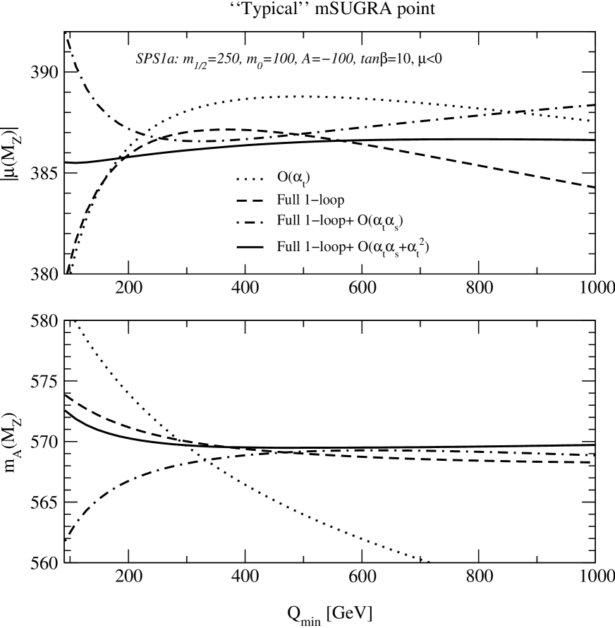
Figure 3: The $\overline{\rm DR}$ parameters $|\mu(M_{\scriptscriptstyle Z})|$ (upper plot) and $m_{\scriptscriptstyle A}(M_{\scriptscriptstyle Z})$ (lower plot) as a function of the scale $Q_{\rm min}$ at which the minimization conditions of the effective potential are imposed. The input parameters of the mSUGRA scenario are chosen as in the Snowmass Point SPS 1a [19]. The meaning of the different curves is shown in the caption and explained in the text. The mass of the top quark is taken to be 174.3 GeV.

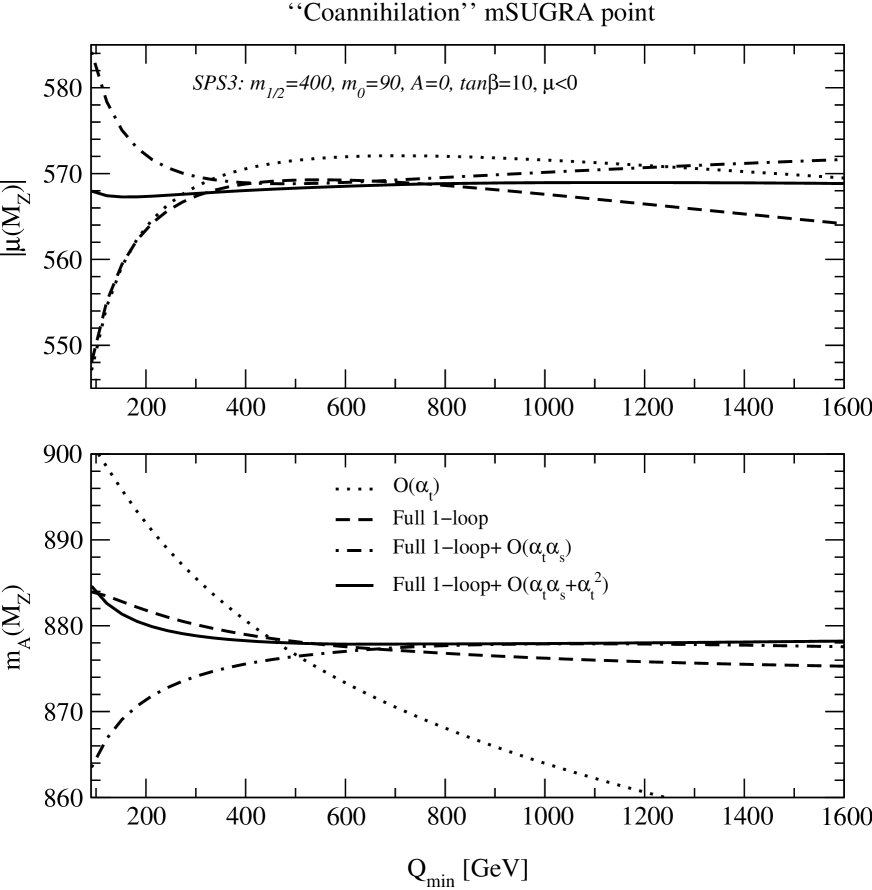
Figure 4: Same as Fig. 3 for the Snowmass Point SPS 3.

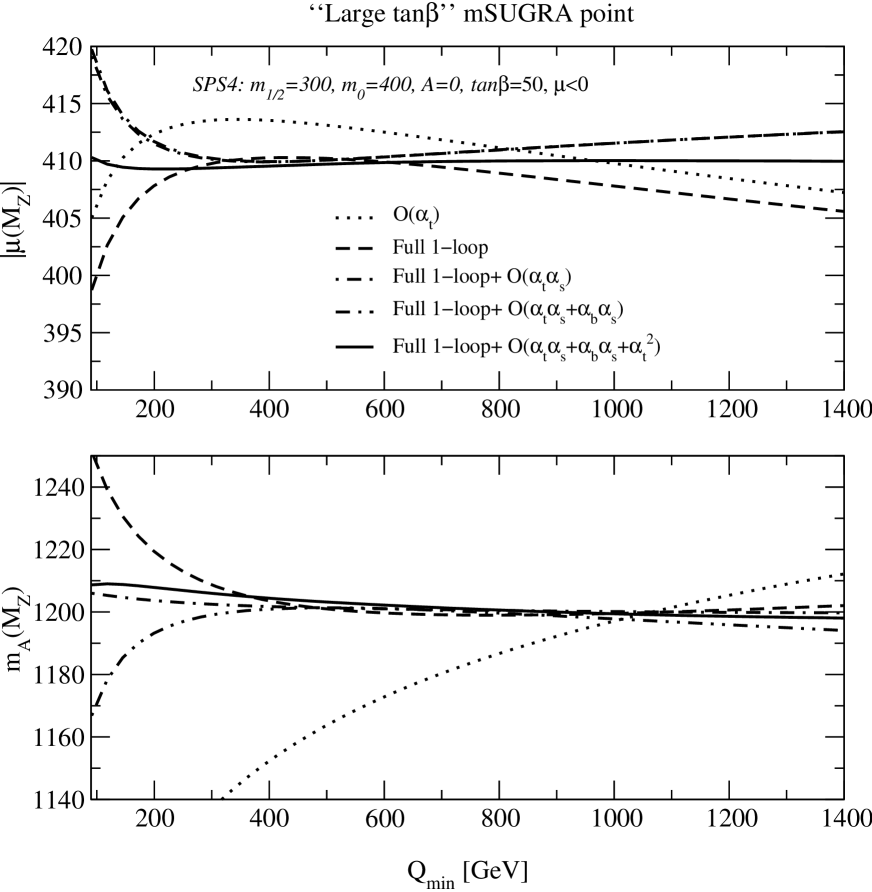
Figure 5: Same as Fig. 3 for the Snowmass Point SPS 4.

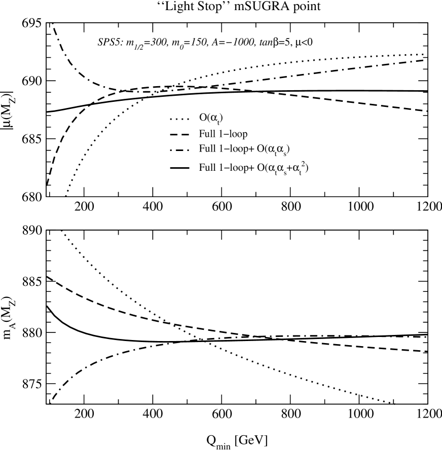
Figure 6: Same as Fig. 3 for the Snowmass Point SPS 5.

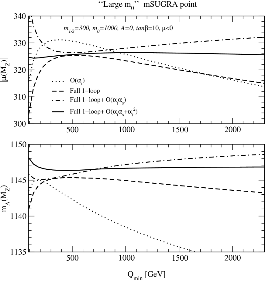
Figure 7: Same as Fig. 3 for the “Large $m_{0}$” mSUGRA point proposed in section 4.

In order to discuss the effect of our ${\cal O}(\alpha_{t}\alpha_{s}+\alpha_{t}^{2})$ corrections to the REWSB conditions, we show in Figs. 3–7 the values of $|\mu(M_{\scriptscriptstyle Z})|$ and $m_{\scriptscriptstyle A}(M_{\scriptscriptstyle Z})$, the latter obtained through $m_{\scriptscriptstyle A}^{2}(M_{\scriptscriptstyle Z})=-2\,m_{3}^{2}(M_{\scriptscriptstyle Z})/\sin 2\beta\,$, as functions of the minimization scale $Q_{\rm min}$. Stability of the results with respect to moderate changes in $Q_{\rm min}$ (which should anyway lie in the weak range, i.e. between $M_{\scriptscriptstyle Z}$ and a few TeV) indicates that the higher–order corrections not included in the computation of $\mu$ and $m_{\scriptscriptstyle A}$ are small and can be safely neglected. We will see that in general the inclusion of our ${\cal O}(\alpha_{t}\alpha_{s}+\alpha_{t}^{2})$ corrections significantly improves the scale–dependence of the results.

In the choice of the input parameters, we refer to the so–called Snowmass Points [19], which represent typical “benchmark” scenarios that are commonly investigated in the phenomenological analyses of the mSUGRA parameter space. In particular, Figs. 3–6 correspond to:

$$\begin{array}[]{lccccc}\vspace*{2mm}{\rm SPS\;1a}:&m_{0}=100\;{\rm GeV},&m_{1/2}=250\;{\rm GeV},&A_{0}=-100\;{\rm GeV},&\tan\beta=10\,,&\mu<0\,,\\ \vspace*{2mm}{\rm SPS\;3}:&m_{0}=90\;{\rm GeV},&m_{1/2}=400\;{\rm GeV},&A_{0}=0\,,&\tan\beta=10\,,&\mu<0\,,\\ \vspace*{2mm}{\rm SPS\;4}:&m_{0}=400\;{\rm GeV},&m_{1/2}=300\;{\rm GeV},&A_{0}=0\,,&\tan\beta=50\,,&\mu<0\,,\\ \vspace*{2mm}{\rm SPS\;5}:&m_{0}=150\;{\rm GeV},&m_{1/2}=300\;{\rm GeV},&A_{0}=-1\;{\rm TeV}\,,&\tan\beta=5\,,&\mu<0\,,\end{array}$$

respectively. Notice that our convention for the sign of $\mu$ differs from the one in Ref. [19], where a discussion on the characteristics of the various scenarios can be found. A further scenario, denoted as “Focus point” (SPS2) and characterized by a common scalar mass, $m_{0}=1450$ GeV, much larger than the common fermion mass, $m_{1/2}=300$ GeV, has also been suggested in Ref. [19]. However, we found that in this scenario the results for $\mu$ and $m_{\scriptscriptstyle A}$, including the qualitative effect of the various corrections and the occurrence of REWSB itself, depend dramatically on very small adjustments of the input value for the top pole mass (e.g. $|\mu(M_{\scriptscriptstyle Z})|$ varies roughly between 400 and 100 GeV if $M_{t}$ is varied between 174.3 and 175 GeV). The extreme sensitivity of the SPS2 scenario on the input top mass has already been discussed in Ref. [25]. Since this scenario appears to lead to unstable results, we will not consider it further in this work. However, in order to investigate the situation in which the common scalar mass is considerably larger than the common fermion mass, we show in Fig. 7 a scenario with $m_{0}=1$ TeV and $m_{1/2}=300$ GeV (the other parameters being chosen as $A_{0}=0\,,\,\tan\beta=10$ and $\mu<0$). We have checked that this “Large $m_{0}$” scenario is not unreasonably sensitive to small variations in the input top mass.

In all the plots of Figs. 3–7 the minimization scale varies in the range $M_{\scriptscriptstyle Z}<Q_{\rm min}<2\,Q_{*}$, where $Q_{*}\equiv(m_{0}^{2}+4\,m_{1/2}^{2})^{1/2}$ is a scale roughly comparable with the squark masses. The dotted curves in the upper and lower panels of each figure represent $|\mu(M_{\scriptscriptstyle Z})|$ and $m_{\scriptscriptstyle A}(M_{\scriptscriptstyle Z})$, respectively, as obtained by including in the minimization conditions only the one–loop ${\cal O}(\alpha_{t})$ top/stop contributions to $\Sigma_{1}$ and $\Sigma_{2}$; the dashed lines include instead the full one–loop computation of $\Sigma_{1}$ and $\Sigma_{2}$; the dot–dashed lines include in addition the two–loop ${\cal O}(\alpha_{t}\alpha_{s})$ contributions; finally, the solid lines include our full two–loop result, i.e. the ${\cal O}(\alpha_{t}\alpha_{s}+\alpha_{t}^{2})$ contributions to $\Sigma_{1}$ and $\Sigma_{2}$. In Fig. 5, corresponding to the “large $\tan\beta$” (SPS4) scenario with $\tan\beta=50$, we show also the effect of the ${\cal O}(\alpha_{b}\alpha_{s})$ corrections, obtained from the ${\cal O}(\alpha_{t}\alpha_{s})$ ones as described at the end of the previous section. The dot–dot–dashed lines in Fig. 5 include the ${\cal O}(\alpha_{t}\alpha_{s}+\alpha_{b}\alpha_{s})$ contributions, while the solid lines represent the full ${\cal O}(\alpha_{t}\alpha_{s}+\alpha_{b}\alpha_{s}+\alpha_{t}^{2})$ result. The effect of the ${\cal O}(\alpha_{b}\alpha_{s})$ corrections is indeed negligible in the other SPS scenarios, where $\tan\beta$ takes on more moderate values. In any case we include the ${\cal O}(\alpha_{b}\alpha_{s})$ corrections in all the scenarios we investigate here.

We see from Figs. 3–7 that the inclusion of the two–loop ${\cal O}(\alpha_{t}\alpha_{s}+\alpha_{t}^{2})$ corrections improves the dependence of $|\mu(M_{\scriptscriptstyle Z})|$ and $m_{\scriptscriptstyle A}(M_{\scriptscriptstyle Z})$ on the minimization scale with respect to the full one–loop result. The effect is particularly manifest in the case of $\mu$, where, in all the scenarios, the two–loop corrected result appears to depend only very weakly (within 3 GeV at most) on $Q_{\rm min}$, while the one–loop result tends to decrease for both small and large $Q_{\rm min}$. In the case of $m_{\scriptscriptstyle A}$, the improvement is less striking: although the two–loop corrected result has in general a better scale dependence than its one–loop counterpart, especially for increasing values of $Q_{\rm min}$, a small residual scale dependence is visible in most plots when $Q_{\rm min}$ gets close to $M_{\scriptscriptstyle Z}$. In any scenario the residual uncertainty on $m_{\scriptscriptstyle A}$ is never larger than 10 GeV (the latter case occurring in the “large $\tan\beta$” scenario, where $m_{\scriptscriptstyle A}(M_{\scriptscriptstyle Z})$ is around 1200 GeV) and might be due to the corrections that we neglect in our two–loop computation of the tadpoles, i.e. those controlled by the electroweak gauge couplings and, for large $\tan\beta$, those of ${\cal O}(\alpha_{b}^{2}+\alpha_{t}\alpha_{b})\,$. From the small residual scale dependence visible in Figs. 3–7, we estimate that the effect of the neglected two–loop and higher–order corrections on the parameters $\mu$ and $m_{\scriptscriptstyle A}$ should be at most of 1%.

Other interesting observations can be drawn from Figs. 3–7: first of all, at the one–loop level, the inclusion of the top/stop contributions only is in general not a good approximation of the full result (this has been already observed e.g. in Ref. [35]). Moreover, at the two–loop level, a significant compensation occurs between the ${\cal O}(\alpha_{t}\alpha_{s})$ and the ${\cal O}(\alpha_{t}^{2})$ contributions to the tadpoles, thus including only the former may lead to rather inaccurate predictions (as shown by the dot–dashed curves). This partial cancellation between the ${\cal O}(\alpha_{t}\alpha_{s})$ and ${\cal O}(\alpha_{t}^{2})$ corrections is similar to the one occurring in the case of the Higgs masses [10, 11, 12]. Finally, it is worth noticing that in the “large $\tan\beta$” scenario of Fig. 5 the inclusion of the ${\cal O}(\alpha_{b}\alpha_{s})$ corrections to the tadpoles has a sizeable effect on the minimization scale dependence of $m_{\scriptscriptstyle A}(M_{\scriptscriptstyle Z})$ (see the difference between the dot–dashed and dot–dot–dashed curves), while it does not affect significantly that of $|\mu(M_{\scriptscriptstyle Z})|$.

It is clear from the above discussion that the numerical effect on $|\mu(M_{\scriptscriptstyle Z})|$ and $m_{\scriptscriptstyle A}(M_{\scriptscriptstyle Z})$ of the two–loop corrections to $\Sigma_{1}$ and $\Sigma_{2}$ depends critically on the choice of the minimization scale. In all the plots we find a range of values of $Q_{\rm min}$, usually in the vicinity of $Q_{*}$, for which the one–loop and two–loop curves are close to each other, implying that the effect of the ${\cal O}(\alpha_{t}\alpha_{s}+\alpha_{t}^{2})$ corrections is small. On the other hand, for values of $Q_{\rm min}$ far from this optimal choice, the omission of the two–loop corrections can lead to an error of several (possibly, tenths of) GeV, especially in the case of $\mu$. Thus, the proper inclusion the ${\cal O}(\alpha_{t}\alpha_{s}+\alpha_{t}^{2})$ two–loop tadpole corrections on the top of the full one–loop ones allows us to obtain more precise and reliable results for $\mu$ and $m_{\scriptscriptstyle A}$, i.e. results that do not depend on a preconceived choice of the minimization scale for the MSSM effective potential.

5 Conclusions

In this paper we presented explicit and general results for the ${\cal O}(\alpha_{t}\alpha_{s}+\alpha_{t}^{2})$ two–loop corrections to the minimization conditions of the MSSM effective potential, which translate into corrections to the $\overline{\rm DR}$–renormalized parameters $\mu$ and $m_{\scriptscriptstyle A}$. We discussed the numerical impact of our corrections in some representative scenarios of gravity–mediated SUSY breaking, and we found that the inclusion of the ${\cal O}(\alpha_{t}\alpha_{s}+\alpha_{t}^{2})$ corrections significantly improves the renormalization scale dependence of the results. Due to partial cancellations between the ${\cal O}(\alpha_{t}\alpha_{s})$ and ${\cal O}(\alpha_{t}^{2})$ corrections, including only the former may lead to inaccurate results. Our corrections are also required for consistency in the ${\cal O}(\alpha_{t}\alpha_{s}+\alpha_{t}^{2})$ two–loop computations of the MSSM Higgs masses, if the parameters entering the tree–level Higgs mass matrix are computed via renormalization group evolution from a set of high energy boundary conditions.

A complete study of the electroweak symmetry breaking at the two–loop level would require also the knowledge of the corrections that are neglected in our gaugeless limit, among which the most relevant are controlled by the bottom Yukawa coupling and the electroweak gauge couplings. Concerning the corrections controlled by $\alpha_{b}$, they can be numerically non–negligible only for large values of $\tan\beta$. As discussed at the end of section 3, the formulae for the ${\cal O}(\alpha_{b}\alpha_{s})$ corrections can be obtained by performing simple substitutions in their ${\cal O}(\alpha_{t}\alpha_{s})$ counterparts. On the other hand, the ${\cal O}(\alpha_{b}^{2}+\alpha_{t}\alpha_{b})$ corrections, which in some cases might be as relevant as the ${\cal O}(\alpha_{b}\alpha_{s})$ ones, cannot be obtained in a straightforward way from the presently computed corrections and would require further work.

In Ref. [17] a complete two–loop computation of the MSSM effective potential is presented, including also the terms controlled by the electroweak gauge couplings that are neglected in our analysis. The inclusion of such terms improves further the scale dependence of the parameters $\mu$ and $m_{\scriptscriptstyle A}$, that in Ref. [17] are determined through a numerical minimization of the effective potential. However, the explicit analytical formulae for the two–loop tadpoles $\Sigma_{1}$ and $\Sigma_{2}$, which are usually needed for practical applications, would be quite involved in the general case, and have not been presented so far.

In conclusion, our work should lead to a more precise and reliable determination of the MSSM parameters at the weak scale, once the boundary conditions are provided at some larger scale according to the underlying theory of SUSY breaking. The fact that, among its many attractive features, the MSSM provides a natural mechanism for breaking radiatively the electroweak symmetry, with the heavy top quark mass nicely falling in the required range, seems to indicate the MSSM as the most viable theory for physics at the weak scale. However, only the forthcoming experimental results from the Tevatron and the LHC will tell us if this is indeed the case.

Appendix A: Two–loop integrals

We give here explicit expressions for the momentum integrals that appear in the two-loop part of the effective potential. The basic integrals in $d=4-2\epsilon$ dimensions are:

$$\frac{1\;\;}{(16\,\pi^{2})^{2}}\,J(x,y) \equiv -\frac{\mu^{2(4-d)}}{(2\pi)^{2d}}\,\int\!\int\,\frac{{\rm d}^{d}p\,{\rm d}^{d}q}{[p^{2}-x][q^{2}-y]}\,,$$ (A1)

$$\frac{1}{(16\,\pi^{2})^{2}}\,I(x,y,z) \equiv \frac{\mu^{2(4-d)}}{(2\pi)^{2d}}\,\int\!\int\,\frac{{\rm d}^{d}p\,{\rm d}^{d}q}{[p^{2}-x][q^{2}-y][(p-q)^{2}-z]}\,.$$ (A2)

Following Ref. [29], the functions $J(x,y)$ and $I(x,y,z)$ defined in Eqs. (A1)–(A2) are:

$$J(x,y) = \frac{xy}{\epsilon^{2}}-\frac{xy}{\epsilon}\,\left(\overline{\ln}x+\overline{\ln}y-2\right)-xy\,\left[2\,\overline{\ln}x+2\,\overline{\ln}y-\frac{1}{2}\,\overline{\ln}^{\,2}xy-\left(3+\frac{\pi^{2}}{6}\right)\,\right]\,,$$ (A3)

$$I(x,y,z) = -\frac{x+y+z}{2\epsilon^{2}}\;+\;\frac{1}{\epsilon}\left[x\,\overline{\ln}x+y\,\overline{\ln}y+z\,\overline{\ln}z-\frac{3}{2}\,(x+y+z)\right]$$ (A4)

$$+\frac{1}{2}\,(x\,\overline{\ln}y\,\overline{\ln}z+y\,\overline{\ln}x\,\overline{\ln}z+z\,\overline{\ln}x\,\overline{\ln}y)-\frac{x+y+z}{2}\,(7+\pi^{2}/6)$$

$$-\frac{1}{2}\,(x\,\overline{\ln}x+y\,\overline{\ln}y+z\,\overline{\ln}z)\,(\overline{\ln}x+\overline{\ln}y+\overline{\ln}z-6)-\frac{\Delta(x,y,z)}{2z}\,\Phi(x,y,z)\,.$$

In the above formulae, $\overline{\ln}x$ stands for $\ln(x/Q^{2})$, where $Q^{2}=4\pi\mu^{2}e^{-\gamma_{E}}$ is the renormalization scale ($\gamma_{E}$ is the Euler constant). The functions $\Delta$ and $\Phi$ are respectively:

$$\Delta(x,y,z) = x^{2}+y^{2}+z^{2}-2\,(xy+xz+yz)\,,$$ (A5)

$$\Phi\,(x,y,z) = \frac{1}{\lambda}\left[2\,\ln x_{+}\,\ln x_{-}-\ln u\,\ln v-2\,\biggr{(}{\rm Li}_{2}(x_{+})+{\rm Li}_{2}(x_{-})\biggr{)}+\frac{\pi^{2}}{3}\right]\,,$$ (A6)

where ${\rm Li}_{2}(z)=-\int_{0}^{z}{\rm d}t\left[\ln(1-t)/t\right]$ is the dilogarithm function and the auxiliary (complex) variables are:

$$u=\frac{x}{z}\,,\;\;\;\;\;\;v=\frac{y}{z}\,,\;\;\;\;\;\;\lambda=\sqrt{(1-u-v)^{2}-4\,u\,v}\,,\;\;\;\;\;\;x_{\pm}=\frac{1}{2}\,\left[1\pm(u-v)-\lambda\right]\,.$$ (A7)

The definition (A6) is valid for the case $x/z<1$ and $y/z<1$. The other branches of $\Phi$ can be obtained using the symmetry properties:

$$\Phi\,(x,y,z)=\Phi\,(y,x,z)\,,\hskip 28.45274ptx\,\Phi\,(x,y,z)=z\,\Phi\,(z,y,x)\,.$$ (A8)

Finally, the following recursive relation for the derivatives of $\Phi$ proved very useful  for obtaining compact analytical results:

$$\Delta(x,y,z)\,\frac{\partial\,\Phi(x,y,z)}{\partial\,x}=(y+z-x)\,\Phi(x,y,z)+\frac{z}{x}\,\left[(y-z)\,\ln\frac{z}{y}+x\,\left(\ln\frac{x}{y}+\ln\frac{x}{z}\right)\,\right]\,.$$ (A9)

The derivatives of $\Phi$ with respect to $y$ and $z$ can be obtained from the above equation with the help of the symmetry properties of Eq. (A8).

Appendix B: Explicit formulae for the ${\cal O}(\alpha_{t}\alpha_{s})$ corrections

We present here explicit expressions for the two–loop part of the functions $F$ and $G$, giving rise to ${\cal O}(\alpha_{t}\alpha_{s})$ corrections to $\Sigma_{1}$ and $\Sigma_{2}$. These formulae are valid when the parameters entering the one–loop parts of $F$ and $G$ are expressed in the $\overline{\rm DR}$ scheme and computed at the renormalization scale $Q$. In units of $g_{s}^{2}\,C_{F}\,N_{c}/(16\pi^{2})^{2}$, where $C_{F}=4/3$ and $N_{c}=3$ are color factors, $F^{2\ell}$ and $G^{2\ell}$ read:

$$F^{2\ell} = \frac{4\,m_{\tilde{g}}\,m_{t}}{s_{2\theta}}\,(1+4\,c_{2\theta}^{2})-\left[2\,(m_{\tilde{t}_{1}}^{2}-m_{\tilde{t}_{2}}^{2})+\frac{4\,m_{\tilde{g}}\,m_{t}}{s_{2\theta}}\right]\,\ln\frac{m_{\tilde{g}}^{2}}{Q^{2}}\,\ln\frac{m_{t}^{2}}{Q^{2}}$$ (B1)

$$-2\,(4-s_{2\theta}^{2})\,(m_{\tilde{t}_{1}}^{2}-m_{\tilde{t}_{2}}^{2})+\frac{4\,m_{\tilde{t}_{1}}^{2}\,m_{\tilde{t}_{2}}^{2}-s_{2\theta}^{2}\,(m_{\tilde{t}_{1}}^{2}+m_{\tilde{t}_{2}}^{2})^{2}}{m_{\tilde{t}_{1}}^{2}-m_{\tilde{t}_{2}}^{2}}\,\ln\frac{m_{\tilde{t}_{1}}^{2}}{Q^{2}}\,\ln\frac{m_{\tilde{t}_{2}}^{2}}{Q^{2}}$$

$$+ \left\{\hskip 8.5359pt\left[4\,(m_{\tilde{g}}^{2}+m_{t}^{2}+2\,m_{\tilde{t}_{1}}^{2})-s_{2\theta}^{2}\,(3\,m_{\tilde{t}_{1}}^{2}+m_{\tilde{t}_{2}}^{2})-\frac{16\,c_{2\theta}^{2}\,m_{\tilde{g}}\,m_{t}\,m_{\tilde{t}_{1}}^{2}}{s_{2\theta}\,(m_{\tilde{t}_{1}}^{2}-m_{\tilde{t}_{2}}^{2})}-4\,s_{2\theta}\,m_{\tilde{g}}\,m_{t}\right]\,\ln\frac{m_{\tilde{t}_{1}}^{2}}{Q^{2}}\right.$$

$$+\frac{m_{\tilde{t}_{1}}^{2}}{m_{\tilde{t}_{1}}^{2}-m_{\tilde{t}_{2}}^{2}}\,\left[s_{2\theta}^{2}\,(m_{\tilde{t}_{1}}^{2}+m_{\tilde{t}_{2}}^{2})-2\,(2\,m_{\tilde{t}_{1}}^{2}-m_{\tilde{t}_{2}}^{2})\right]\,\ln^{2}\frac{m_{\tilde{t}_{1}}^{2}}{Q^{2}}$$

$$+2\,\left[m_{\tilde{t}_{1}}^{2}-m_{\tilde{g}}^{2}-m_{t}^{2}+m_{\tilde{g}}\,m_{t}\,s_{2\theta}+\frac{2\,c_{2\theta}^{2}\,m_{\tilde{g}}\,m_{t}\,m_{\tilde{t}_{1}}^{2}}{s_{2\theta}\,(m_{\tilde{t}_{1}}^{2}-m_{\tilde{t}_{2}}^{2})}\right]\,\ln\frac{m_{\tilde{g}}^{2}\,m_{t}^{2}}{Q^{4}}\,\ln\frac{m_{\tilde{t}_{1}}^{2}}{Q^{2}}$$

$$+\frac{4\,m_{\tilde{g}}\,m_{t}\,c_{2\theta}^{2}\,(m_{t}^{2}-m_{\tilde{g}}^{2})}{s_{2\theta}\,(m_{\tilde{t}_{1}}^{2}-m_{\tilde{t}_{2}}^{2})}\,\ln\frac{m_{t}^{2}}{m_{\tilde{g}}^{2}}\,\ln\frac{m_{\tilde{t}_{1}}^{2}}{Q^{2}}+\left[\frac{4\,m_{\tilde{g}}^{2}\,m_{t}^{2}+2\,\Delta(m_{\tilde{g}}^{2},m_{t}^{2},m_{\tilde{t}_{1}}^{2})}{m_{\tilde{t}_{1}}^{2}}\right.$$

$$\left.-\frac{2\,m_{\tilde{g}}\,m_{t}\,s_{2\theta}}{m_{\tilde{t}_{1}}^{2}}\,(m_{\tilde{g}}^{2}+m_{t}^{2}-m_{\tilde{t}_{1}}^{2})+\frac{4\,c_{2\theta}^{2}\,m_{\tilde{g}}\,m_{t}\,\Delta(m_{\tilde{g}}^{2},m_{t}^{2},m_{\tilde{t}_{1}}^{2})}{s_{2\theta}\,m_{\tilde{t}_{1}}^{2}\,(m_{\tilde{t}_{1}}^{2}-m_{\tilde{t}_{2}}^{2})}\,\right]\,\Phi(m_{\tilde{g}}^{2},m_{t}^{2},m_{\tilde{t}_{1}}^{2})$$

$$\left.\hskip 142.26378pt\phantom{\ln^{2}\frac{m_{\tilde{t}_{1}}^{2}}{Q^{2}}}-(m_{\tilde{t}_{1}}^{2}\leftrightarrow m_{\tilde{t}_{2}}^{2}\,,\;s_{2\theta}\rightarrow-s_{2\theta})\;\;\right\}\,,$$

$$G^{2\ell} = \frac{5\,m_{\tilde{g}}\,s_{2\theta}}{m_{t}}\,(m_{\tilde{t}_{1}}^{2}-m_{\tilde{t}_{2}}^{2})-10\,(m_{\tilde{t}_{1}}^{2}+m_{\tilde{t}_{2}}^{2}-2\,m_{t}^{2})-4\,m_{\tilde{g}}^{2}+12\,m_{t}^{2}\,\left(\ln^{2}\frac{m_{t}^{2}}{Q^{2}}-2\ln\frac{m_{t}^{2}}{Q^{2}}\right)$$ (B2)

$$+\left[4\,m_{\tilde{g}}^{2}-\frac{m_{\tilde{g}}\,s_{2\theta}}{m_{t}}\,(m_{\tilde{t}_{1}}^{2}-m_{\tilde{t}_{2}}^{2})\right]\,\ln\frac{m_{\tilde{g}}^{2}}{Q^{2}}\,\ln\frac{m_{t}^{2}}{Q^{2}}+s_{2\theta}^{2}\,(m_{\tilde{t}_{1}}^{2}+m_{\tilde{t}_{2}}^{2})\,\ln\frac{m_{\tilde{t}_{1}}^{2}}{Q^{2}}\,\ln\frac{m_{\tilde{t}_{2}}^{2}}{Q^{2}}$$

$$+ \left\{\hskip 8.5359pt\left[4\,(m_{\tilde{g}}^{2}+m_{t}^{2}+2\,m_{\tilde{t}_{1}}^{2})+s_{2\theta}^{2}\,(m_{\tilde{t}_{1}}^{2}-m_{\tilde{t}_{2}}^{2})-\frac{4\,m_{\tilde{g}}\,s_{2\theta}}{m_{t}}\,(m_{t}^{2}+m_{\tilde{t}_{1}}^{2})\right]\,\ln\frac{m_{\tilde{t}_{1}}^{2}}{Q^{2}}\right.$$

$$+\left[\frac{m_{\tilde{g}}\,s_{2\theta}}{m_{t}}\,(5\,m_{t}^{2}-m_{\tilde{g}}^{2}+m_{\tilde{t}_{1}}^{2})-2\,(m_{\tilde{g}}^{2}+2\,m_{t}^{2})\right]\,\ln\frac{m_{t}^{2}}{Q^{2}}\,\ln\frac{m_{\tilde{t}_{1}}^{2}}{Q^{2}}$$

$$+\left[\frac{m_{\tilde{g}}\,s_{2\theta}}{m_{t}}\,(m_{\tilde{g}}^{2}-m_{t}^{2}+m_{\tilde{t}_{1}}^{2})-2\,m_{\tilde{g}}^{2}\right]\,\ln\frac{m_{\tilde{g}}^{2}}{Q^{2}}\,\ln\frac{m_{\tilde{t}_{1}}^{2}}{Q^{2}}-(2+s_{2\theta}^{2})\,m_{\tilde{t}_{1}}^{2}\,\ln^{2}\frac{m_{\tilde{t}_{1}}^{2}}{Q^{2}}$$

$$+\left[2\,\frac{m_{\tilde{g}}^{2}}{m_{\tilde{t}_{1}}^{2}}\,(m_{\tilde{g}}^{2}+m_{t}^{2}-m_{\tilde{t}_{1}}^{2}-2\,m_{\tilde{g}}\,m_{t}\,s_{2\theta})+\frac{m_{\tilde{g}}\,s_{2\theta}}{m_{t}\,m_{\tilde{t}_{1}}^{2}}\,\Delta(m_{\tilde{g}}^{2},m_{t}^{2},m_{\tilde{t}_{1}}^{2})\right]\,\Phi(m_{\tilde{g}}^{2},m_{t}^{2},m_{\tilde{t}_{1}}^{2})$$

$$\left.\hskip 142.26378pt\phantom{\ln^{2}\frac{m_{\tilde{t}_{1}}^{2}}{Q^{2}}}+(m_{\tilde{t}_{1}}^{2}\leftrightarrow m_{\tilde{t}_{2}}^{2}\,,\;s_{2\theta}\rightarrow-s_{2\theta})\;\;\right\}\,.$$

The functions $\Delta(x,y,z)$ and $\Phi(x,y,z)$ appearing in $F^{2\ell}$ and $G^{2\ell}$ are defined in Eqs. (A5)–(A6). The parameter $s_{2\theta}$ is defined in Eq. (13).

Figure 2: The classes of Feynman diagrams that contribute to the two–loop effective potential and affect the ${\cal O}(\alpha_{t}^{2})$ corrections to the electroweak symmetry breaking conditions [$q=(t,b)$, $\varphi=(H,h,G,A,H^{\pm},G^{\pm})$, $\tilde{h}=(\tilde{h}^{0},\tilde{h}^{\pm})$, $\tilde{q}=(\tilde{t}_{1},\tilde{t}_{2},\tilde{b}_{L})$].

References

-
[1]
H. P. Nilles, Phys. Rept. 110 (1984) 1;
H. E. Haber and G. L. Kane, Phys. Rept. 117 (1985) 75;
A. B. Lahanas and D. V. Nanopoulos, Phys. Rept. 145 (1987) 1;
for a more recent review and further references see S. P. Martin, hep-ph/9709356. - [2] L. E. Ibanez and G. G. Ross, Phys. Lett. B110 (1982) 215.
-
[3]
K. Inoue, A. Kakuto, H. Komatsu and S. Takeshita,
Prog. Theor. Phys. 68, 927 (1982) and Erratum, ibid. 70 (1983) 330;
Prog. Theor. Phys. 71 (1984) 413;
L. Alvarez-Gaumé, M. Claudson and M. B. Wise, Nucl. Phys. B207 (1982) 96;
L. Alvarez-Gaumé, J. Polchinski and M. B. Wise, Nucl. Phys. B221 (1983) 495;
J. R. Ellis, J. S. Hagelin, D. V. Nanopoulos and K. Tamvakis, Phys. Lett. B125 (1983) 275. -
[4]
S. R. Coleman and E. Weinberg,
Phys. Rev. D7 (1973) 1888;
S. Weinberg, Phys. Rev. D7 (1973) 2887;
R. Jackiw, Phys. Rev, D9 (1974) 1686. - [5] C. Kounnas, A. B. Lahanas, D. V. Nanopoulos and M. Quirós, Nucl. Phys. B236 (1984) 438.
- [6] G. Gamberini, G. Ridolfi and F. Zwirner, Nucl. Phys. B331 (1990) 331.
-
[7]
R. Arnowitt and P. Nath, Phys. Rev. D46 (1992) 3981;
V. D. Barger, M. S. Berger and P. Ohmann, Phys. Rev. D49 (1994) 4908 [hep-ph/9311269];
D. M. Pierce, J. A. Bagger, K. T. Matchev and R. J. Zhang, Nucl. Phys. B491 (1997) 3 [hep-ph/9606211];
D. V. Gioutsos, Eur. Phys. J. C17 (2000) 675 [hep-ph/9905278]. -
[8]
D. J. Castaño, E. J. Piard and P. Ramond,
Phys. Rev. D49 (1994) 4882 [hep-ph/9308335];
G. L. Kane, C. Kolda, L. Roszkowski and J. Wells, Phys. Rev. D49 (1994) 6173 [hep-ph/9312272];
A. Dedes, A. B. Lahanas and K. Tamvakis, Phys. Rev. D53 (1996) 3793 [hep-ph/9504239]. -
[9]
J. Ellis, G. Ridolfi and F. Zwirner,
Phys. Lett. B257 (1991) 83;
Phys. Lett. B262 (1991) 477;
A. Brignole, J. Ellis, G. Ridolfi and F. Zwirner, Phys. Lett. B271 (1991) 123 and Erratum, ibid. B273 (1991) 550;
M. Drees and M. M. Nojiri, Phys. Rev. D45 (1992) 2482. - [10] R. Hempfling and A. H. Hoang, Phys. Lett. B331 (1994) 99 [hep-ph/9401219].
-
[11]
R. Zhang, Phys. Lett. B447 (1999) 89 [hep-ph/9808299];
J. R. Espinosa and R. Zhang, JHEP 0003 (2000) 026 [hep-ph/9912236]; Nucl. Phys. B586 (2000) 3 [hep-ph/0003246]. -
[12]
G. Degrassi, P. Slavich and F. Zwirner,
Nucl. Phys. B611 (2001) 403 [hep-ph/0105096];
A. Brignole, G. Degrassi, P. Slavich and F. Zwirner, Nucl. Phys. B631 (2002) 195 [hep-ph/0112177]. - [13] A. Brignole, G. Degrassi, P. Slavich and F. Zwirner, Nucl. Phys. B643 (2002) 79 [hep-ph/0206101].
- [14] S. P. Martin, hep-ph/0211366.
-
[15]
M. Carena, J. R. Espinosa, M. Quiros and C. E. Wagner,
Phys. Lett. B355 (1995) 209 [hep-ph/9504316];
M. Carena, M. Quiros and C. E. Wagner, Nucl. Phys. B461 (1996) 407 [hep-ph/9508343];
H. E. Haber, R. Hempfling and A. H. Hoang, Z. Phys. C75 (1997) 539 [hep-ph/9609331];
J. R. Espinosa and I. Navarro, Nucl. Phys. B615 (2001) 82 [hep-ph/0104047]. - [16] S. Heinemeyer, W. Hollik and G. Weiglein, Phys. Rev. D58 (1998) 091701 [hep-ph/9803277]; Phys. Lett. B440 (1998) 296 [hep-ph/9807423]; Eur. Phys. J. C9 (1999) 343 [hep-ph/9812472].
- [17] S. P. Martin, Phys. Rev. D65 (2002) 116003 [hep-ph/0111209]; Phys. Rev. D66 (2002) 096001 [hep-ph/0206136].
-
[18]
H. P. Nilles,
Phys. Lett. B115 (1982) 193;
Nucl. Phys. B217 (1983) 366;
A. H. Chamseddine, R. Arnowitt and P. Nath, Phys. Rev. Lett. 49 (1982) 970;
R. Barbieri, S. Ferrara and C. A. Savoy, Phys. Lett. B119 (1982) 343;
L. Hall, J. Lykken and S. Weinberg, Phys. Rev. D27 (1983) 2359;
S. K. Soni and H. A. Weldon, Phys. Lett. B126 (1983) 215. - [19] B. C. Allanach et al., Eur. Phys. J. C25 (2002) 113 [hep-ph/0202233].
- [20] A. Djouadi, J. L. Kneur and G. Moultaka, hep-ph/0211331.
- [21] B. C. Allanach, Comput. Phys. Commun. 143 (2002) 305 [hep-ph/0104145].
- [22] W. Porod, hep-ph/0301101.
- [23] A. Dedes, G. Weiglein and S. Heinemeyer, in Les Houches 2001, Physics at TeV colliders, p. 134–137.
- [24] H. Baer, F. E. Paige, S. D. Protopopescu and X. Tata, hep-ph/0001086.
- [25] B. C. Allanach, S.Kraml and W. Porod, hep-ph/0207314.
-
[26]
W. Siegel, Phys. Lett. B84 (1979) 193;
D.M. Capper, D.R.T. Jones and P. van Nieuwenhuizen, Nucl. Phys. B167 (1980) 479. - [27] I. Jack, D.R.T. Jones, S.P. Martin, M.T. Vaughn and Y. Yamada, Phys. Rev. D50 (1994) 5481 [hep-ph/9407291].
- [28] C. Ford, I. Jack and D.R.T. Jones, Nucl. Phys. B387 (1992) 373; Erratum ibid. B504 (1997) 551 [hep-ph/0111190].
- [29] A.I. Davydychev and J.B. Tausk, Nucl. Phys. B397 (1993) 123.
-
[30]
S.P. Martin and M.T. Vaughn, Phys. Rev. D50 (1994) 2282 [hep-ph/9311340];
Y. Yamada, Phys. Rev. D50 (1994) 3537 [hep-ph/9401241];
I. Jack and D.R.T. Jones, Phys. Lett. B333 (1994) 372 [hep-ph/9405233]. -
[31]
T. Banks, Nucl. Phys. B303 (1988) 172;
L. J. Hall, R. Rattazzi and U. Sarid, Phys. Rev. D50 (1994) 7048 [hep-ph/9306309];
R. Hempfling, Phys. Rev. D49 (1994) 6168;
M. Carena, M. Olechowski, S. Pokorski and C. E. Wagner, Nucl. Phys. B426 (1994) 269 [hep-ph/9402253]. - [32] M. Carena, D. Garcia, U. Nierste and C. E. Wagner, Nucl. Phys. B577 (2000) 577 [hep-ph/9912516].
- [33] H. Arason, D. J. Castano, B. Keszthelyi, S. Mikaelian, E. J. Piard, P. Ramond and B. D. Wright, Phys. Rev. D46 (1992) 3945.
- [34] Y. Yamada, Phys. Lett. B530 (2002) 174 [hep-ph/0112251].
- [35] A. B. Lahanas and V. C. Spanos, Eur. Phys. J. C23 (2002) 185 [hep-ph/0106345].