Combining first KamLAND results with solar neutrino data

Abstract

We consider the impact of the recent KamLAND data on neutrino oscillations, the first terrestrial neutrino experiment that can probe the solar neutrino anomaly. By combining the first 145.1 days of KamLAND data with the full sample of latest solar neutrino data we find an enhanced rejection against non-LMA oscillations, allowed only at more than $4\sigma$ with respect to LMA. Furthermore, the new data have a strong impact in narrowing down the allowed range of $\Delta m^{2}$ inside the LMA region. In contrast, our global analysis indicates that the new data have little impact on the location of the best fit point. In particular the solar neutrino mixing remains significantly non-maximal ($3\sigma$).

I Introduction

In a recent paper the first results of the KamLAND collaboration became public kamlandPRL . These data contain precious information on the neutrino oscillation hypothesis which has been advocated to account for a number of neutrino experiments involving solar and atmospheric neutrinos and which indicate that neutrinos are massive and that neutrino flavor mixing occurs Fukuda:2001nj ; Fukuda:2002pe ; Fukuda:1998fd ; Fukuda:1998rq ; Cleveland:nv ; Davis:jw ; Abdurashitov:1999zd ; Hampel:1998xg ; Altmann:2000ft ; Cattadori:rd ; sno ; Fukuda:1998mi . The KamLAND experiment is a reactor neutrino experiment with its detector located at the Kamiokande site. Most of the $\bar{\nu}_{e}$ flux incident at KamLAND comes from plants at distances of $80-350$ km from the detector, making the average baseline of about 180 kilometers, long enough to provide a sensitive probe of the LMA solution of the solar neutrino problem MSW ; Bahcall:1999ed ; Gonzalez-Garcia:1999aj . The KamLAND collaboration has for the first time measured the disappearance of neutrinos traveling to a detector from a power reactor. They observe a strong evidence for the disappearance of neutrinos during their flight over such distances, giving the first terrestrial confirmation of the solar neutrino anomaly and also establishing the oscillation hypothesis with man-produced neutrinos. Moreover the parameters that describe this disappearance in terms of the oscillations of the electron neutrino type to another, are consistent with latest pre-KamLAND determinations Maltoni:2002ni ; Bahcall:2002hv ; Bandyopadhyay:2002xj ; Barger:2002iv ; deHolanda:2002pp ; Creminelli:2001ij ; Fogli:2002pt of solar neutrino parameters.

In this note we analyze the implications of these fundamental results by combining the KamLAND data with data from solar neutrino experiments. We will assume CPT conservation and for simplicity we consider a two-flavor massive neutrino oscillation framework. In Sec. II we analyze the impact of the KamLAND results by including the full information on the spectral distribution of the observed events. Subsequently, in Sec. III we perform a global fit that combines the full KamLAND and Chooz reactor data sample Apollonio:1999ae with the full solar neutrino data as included in Ref. Maltoni:2002ni . In Sec. IV we check the stability of the results with respect to changes in the statistical analysis, and we summarize in Sec. V.

II Simulation and analysis of KamLAND data

In KamLAND the target for the $\bar{\nu}_{e}$ flux consists of a spherical transparent balloon filled with 1000 tons of non-doped liquid scintillator. The anti-neutrinos are detected via the inverse neutron $\beta$-decay

$$\bar{\nu}_{e}+p\to e^{+}+n\,.$$ (1)

In Fig. 5 of Ref. kamlandPRL the spectral data are given in 13 bins of prompt energy above 2.6 MeV. To simulate the KamLAND data we calculate the expected number of events in each bin for given oscillation parameters as

$$\begin{split}N_{i}^{\mathrm{th}}(\Delta m^{2},\theta)&=f\int dE_{\nu}\,\sigma(E_{\nu})\times\\ \sum_{j}\phi_{j}(E_{\nu})&P_{j}(E_{\nu},\Delta m^{2},\theta)\int_{i}dE_{e}\,R(E_{e},E^{\prime}_{e})\,.\end{split}$$ (2)

Here $R(E_{e},E_{e}^{\prime})$ is the energy resolution function and $E_{e},E_{e}^{\prime}$ are the observed and the true positron energy, respectively, and we use an energy resolution of $7.5\%/\sqrt{E(\mathrm{MeV})}$ kamlandPRL . The neutrino energy is related to the positron energy by $E_{\nu}=E_{e}^{\prime}+\Delta$, where $\Delta$ is the neutron-proton mass difference. The integration interval over $E_{e}$ is determined by the prompt energy interval in each bin. The neutrino spectrum $\phi(E_{\nu})$ from nuclear reactors is well known, we are using the phenomenological parameterization given in Refs. Vogel:iv ; Murayama:2000iq . We adopt the average fuel composition for the nuclear reactors given in Ref. kamlandPRL . Note that possible effects due to time variations in the fuel composition have been shown to be small Murayama:2000iq . The sum over $j$ in Eq. (2) runs over 16 nuclear plants, taking into account the different distances from the detector and the power output of each reactor (see Table 3 of Ref. kamlandproposal ). The relevant detection cross section $\sigma(E_{\nu})$ is given in Ref. Vogel:1999zy . In the 2-neutrino framework the survival probability for the neutrinos coming from the reactor $j$ is given by

$$P_{j}(E_{\nu},\Delta m^{2},\theta)=1-\sin^{2}2\theta\sin^{2}\frac{\Delta m^{2}L_{j}}{4E_{\nu}}\,.$$ (3)

The normalization factor $f$ in Eq. (2) is determined in such a way that for the case of no oscillations we obtain a total number of events of 86.8, as expected from the Monte-Carlo simulation used in Ref. kamlandPRL .

For the statistical analysis we use the $\chi^{2}$-function

$$\chi^{2}=\sum_{i,j}(N_{i}^{\mathrm{th}}-N_{i}^{\mathrm{obs}})S^{-1}_{ij}(N_{j}^{\mathrm{th}}-N_{j}^{\mathrm{obs}})\,.$$ (4)

The observed number of events $N_{j}^{\mathrm{obs}}$ in each bin can be read off from Fig. 5 of Ref. kamlandPRL . In the covariance matrix $S$ we include the experimental error in each bin $\sigma_{i}$ (obtained from the same figure), which we assume to be uncorrelated, and the systematic error $\sigma_{\mathrm{syst}}=0.0642$ kamlandPRL implied by the uncertainty on the total number of events expected for no oscillations:

$$S_{ij}=\sigma_{i}^{2}\delta_{ij}+\sigma^{2}_{\mathrm{syst}}N_{i}^{\mathrm{th}}N_{j}^{\mathrm{th}}\,.$$ (5)

This $\chi^{2}$ definition assumes Gaussian distribution of the data. For the discussion of an alternative analysis based on poisson distributed data see Sec. IV.

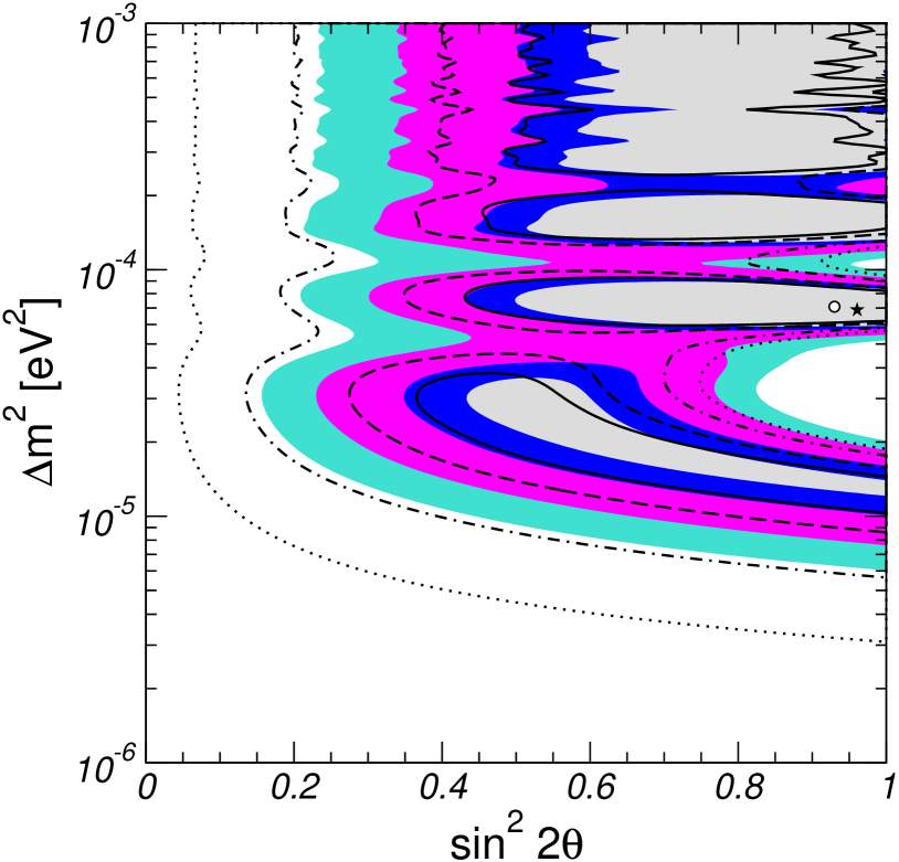
Figure 1: Allowed regions at 90%, 95%, 99% and 99.73% C.L. (2 d.o.f.) and best fit point from KamLAND spectral data. The colored regions and the star are obtained by using the $\chi^{2}$ of Eq. (4) based on the Gaussian approximation, the hollow regions and the dot correspond to the $\chi^{2}$ of Eq. (11) implied by Poisson–distributed data.

III Results and Discussion

Our results are summarized in Figs. 1, 2 and 3. In Fig. 1 we show the allowed regions of the oscillation parameters obtained from our re-analysis of the KamLAND data. It is in good agreement with the analysis performed by the KamLAND group, shown in Fig. 6 of Ref. kamlandPRL . This gives us confidence on our simulation of the KamLAND data and therefore encourages us to use it in a full analysis combining also with the solar data sample. Figs. 2 and 3 show the corresponding results obtained in a combined fit of the full KamLAND data sample with the global sample of solar neutrino data, as well as the Chooz result. The solar data we are using and the details of our solar neutrino analysis are given in Ref. Maltoni:2002ni .

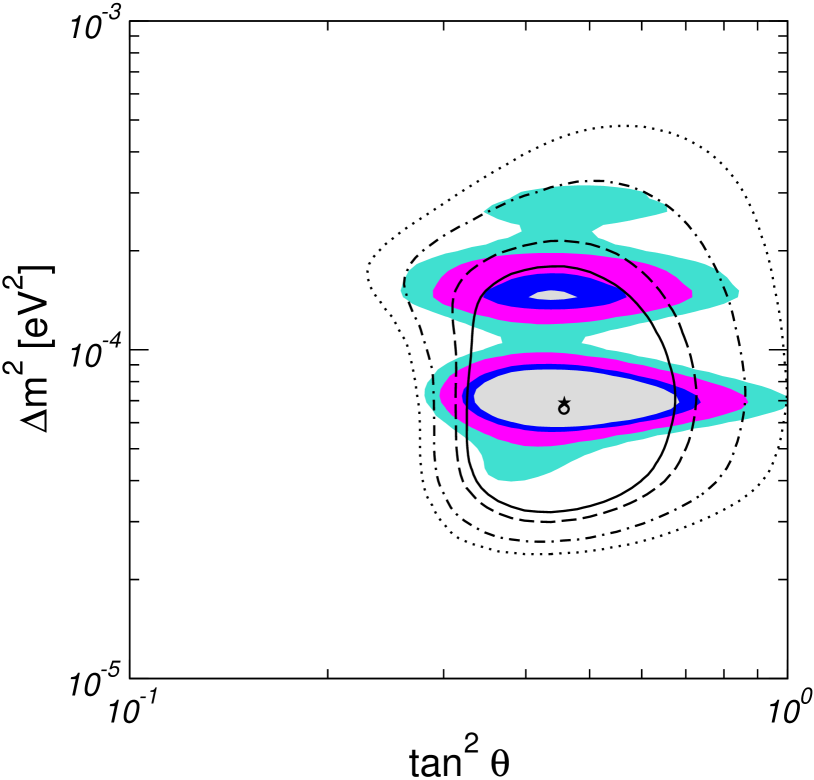
Figure 2: Allowed regions at 90%, 95%, 99% and 99.73% C.L. (2 d.o.f.) from the combined analysis of solar, Chooz and KamLAND data. The hollow lines are the allowed regions from solar and Chooz data alone. The star (dot) is the best fit point from the combined (solar+Chooz only) analysis.

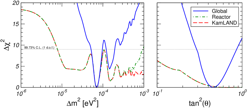
Figure 3: $\Delta\chi^{2}$ versus $\Delta m^{2}$ and $\tan^{2}\theta$. The red dashed line refers to KamLAND alone. The green dot-dashed line corresponds to the full reactor data sample, including both KamLAND and Chooz. The blue solid line refers to the global analysis of the complete solar and reactor data.

First of all, we have quantified the rejection of non-LMA solutions and found that it is now more robust. For example, for the LOW solution we have $\Delta\chi^{2}_{\text{LOW--LMA}}=26.9$, which for 2 d.o.f. ($\Delta m^{2}$ and $\theta$) corresponds to a relative probability of $1.4\times 10^{-6}$, assuming Gaussian errors. A similar result is also found for the VAC solution. Apart from selecting out LMA as the unique solution of the solar neutrino problem we find, however, that the new reactor results have little impact on the location of the best fit point:

$$\tan^{2}\theta=0.46,\qquad\Delta m^{2}=6.9\times 10^{-5}\leavevmode\nobreak\ \text{eV}^{2}.$$ (6)

In particular the solar neutrino mixing remains significantly non-maximal, a point which is rather important for model-building. Indeed bi-maximal mixing models are disfavored Chankowski:2000fp while models where the solar mixing can be non-maximal Babu:2002dz are preferred, as before. This is not in contradiction with the fact that KamLAND data alone prefer maximal mixing kamlandPRL , since such preference has no statistical significance. Indeed, one can see from the right panel in Fig. 3 that $\Delta\chi^{2}$ is rather flat with respect to the mixing angle for $\tan^{2}\theta\gtrsim 0.4$. This explains why the addition of the KamLAND data has no impact whatsoever in the determination of the solar neutrino oscillation mixing. The allowed $3\sigma$ region we find for $\theta$ is:

$$0.29\leq\tan^{2}\theta\leq 0.86,$$ (7)

practically identical to the pre-KamLAND range given in Eq. (4) of Ref. Maltoni:2002ni .

On the other hand, the new data do have a strong impact in narrowing down the allowed range of $\Delta m^{2}$. From the left panel of Fig. 3 one can read off that KamLAND data alone provides the bound $\Delta m^{2}>8\times 10^{-6}\leavevmode\nobreak\ \text{eV}^{2}$, whereas the CHOOZ experiment gives $\Delta m^{2}<10^{-3}\leavevmode\nobreak\ \text{eV}^{2}$, both at $3\sigma$. Hence, global reactor neutrino data provide a robust allowed interval for $\Delta m^{2}$, based only on terrestrial experiments using artificial neutrino sources. However, combining this information from reactors with the solar neutrino data leads to a significant reduction of the allowed range: As clearly visible in Fig. 2, the original LMA region is now split into two sub-regions. From Fig. 3 we obtain at $3\sigma$ (1 d.o.f.)

$$5.1\times 10^{-5}\leavevmode\nobreak\ \text{eV}^{2}\leq\Delta m^{2}\leq 9.7\times 10^{-5}\leavevmode\nobreak\ \text{eV}^{2},$$ (8)

$$1.2\times 10^{-4}\leavevmode\nobreak\ \text{eV}^{2}\leq\Delta m^{2}\leq 1.9\times 10^{-4}\leavevmode\nobreak\ \text{eV}^{2}.$$ (9)

The local minimum in the region (9) occurs for

$$\tan^{2}\theta=0.42,\qquad\Delta m^{2}=1.4\times 10^{-4}\leavevmode\nobreak\ \text{eV}^{2}$$ (10)

with a $\Delta\chi^{2}=4.5$ with respect to the best fit point given in Eq. (6). This ambiguity might be resolved when more KamLAND data have been collected (see e.g. Refs. Murayama:2000iq ; deGouvea:2001su ; Barger:2000hy ).

IV Stability of the statistical analysis

The current KamLAND data sample consists of 54 anti-neutrino events, which are distributed over the 13 energy bins. This leads to rather small numbers of events in each bin. The 5 bins with highest energies contain no event at all. In such a case the use of a $\chi^{2}$-function based on Poisson statistics might be appropriate. In order to check the stability of our results we have performed also an analysis by using pdg

$$\chi^{2}=2\sum_{i}\left[\alpha N_{i}^{\mathrm{th}}-N_{i}^{\mathrm{obs}}+N_{i}^{\mathrm{obs}}\ln\left(\frac{N_{i}^{\mathrm{obs}}}{\alpha N_{i}^{\mathrm{th}}}\right)\right]+\left(\frac{1-\alpha}{\sigma_{\mathrm{syst}}}\right)^{2}$$ (11)

where the term containing the logarithm is absent in bins with no events. We minimize with respect to $\alpha$ in order to take into account the overall uncertainty of the theoretical predictions.

The analysis of KamLAND data using Eq. (11) is shown in Fig. 1 as the hollow lines. We observe that this analysis is somewhat less constraining compared to the analysis based on the Gaussian $\chi^{2}$ of Eq. (4). One notices that smaller values of the mixing angle are allowed, especially at high convidence level. Let us note, however, that the allowed regions from the Gaussian analysis are in better agreement with the analysis done by the KamLAND group. This is the reason why we prefer to use this method for analyzing KamLAND data. The better agreement with the original KamLAND analysis might be related to the fact that the inclusion of the information on the experimental errors provided by the KamLAND collaboration in Fig. 5 of Ref. kamlandPRL can only be included by means of a Gaussian $\chi^{2}$-function, as in Eq. (4). In this way it is possible to take into account the asymmetric errors and the error bars in bins where the number of events is zero.

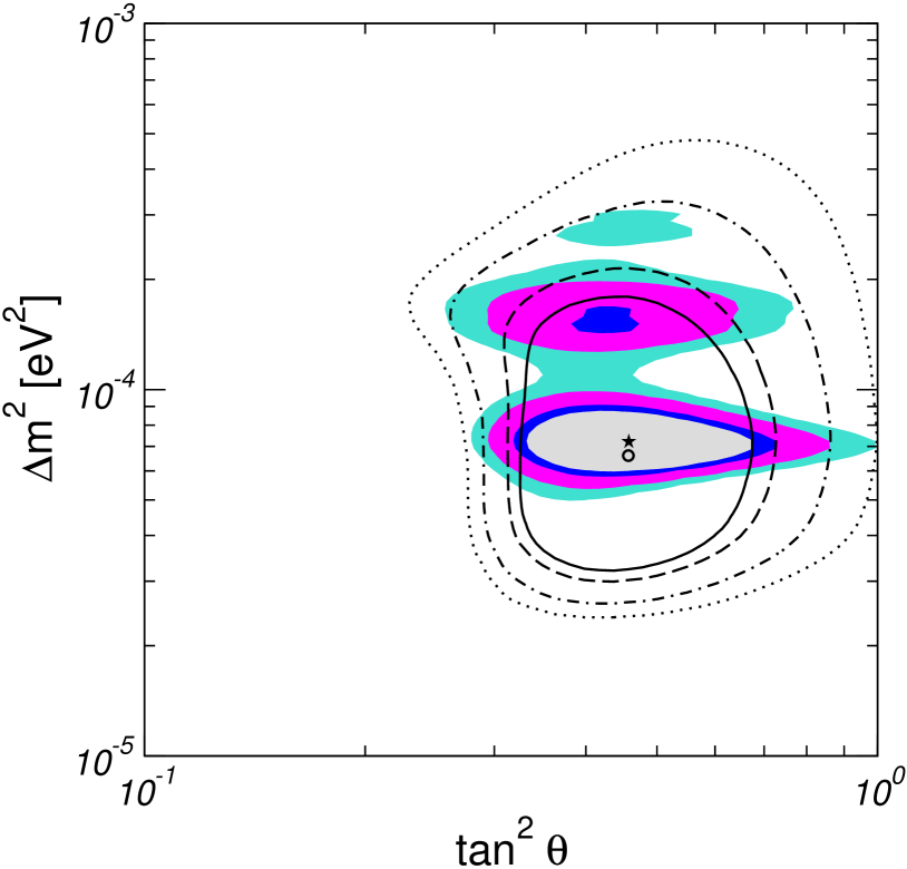
Figure 4: As Fig. 2, but using for the analysis of KamLAND data the $\chi^{2}$ of Eq. (11) implied by Poisson distributed data

However, we note that the determination of $\Delta m^{2}$ is rather stable, only the constraint on the mixing angle is somehow affected. Since the bound on the mixing angle in the combined analysis is dominated by solar data, we expect the difference between the two methods to be small after combining KamLAND with solar data. The results of this exercise are shown in Fig. 4. Comparing this figure with Fig. 2 we find indeed, that the result is very similar. The location of the best fit point and the 90%, 95% and 99% C.L. regions around the best fit point are nearly identical. However, the local minimum does not appear at the 90% C.L., though its location is, again, very stable. Some small differences are visible for the 99.73% C.L. contour.

To summarize, although there are some notable differences between the allowed regions obtained by assuming Gaussian or Poisson $\chi^{2}$-functions for the KamLAND data taken alone, the differences are very small when combined with solar data. This illustrates the robustness of our results against variations in the statistical analysis.

V Conclusions

We find that among all previous oscillation solutions to the solar neutrino anomaly, the new reactor results from the KamLAND experiment single out the LMA solution, rejecting all other oscillation solutions at a significant level. Furthermore, we find that already these first 145.1 days of KamLAND data lead to a significant improvement in narrowing down the allowed range of $\Delta m^{2}$ when combined with solar neutrino data. The original LMA region now is split into two relatively narrow islands around the values of $\Delta m^{2}=6.9\times 10^{-5}$ eV² (best fit point) and $\Delta m^{2}=1.4\times 10^{-4}$ eV² (local minimum). However, our full analysis indicates that the new data have little impact on the determination of the mixing angle. In particular the solar neutrino mixing remains significantly non-maximal ($3\sigma$).

Before closing, let us note that we have considered here only the simplest case of two neutrinos. Analyzing in detail the impact of the KamLAND results on three-neutrino oscillation scenarios Gonzalez-Garcia:2000sq and the resulting constraints is beyond the scope of this short note. The improved determination of $\Delta m^{2}$ can also play an interesting role in probing fine details of solar physics Burgess:2002we , matter effects Fogli:2002hb , probing electro-magnetic neutrino properties Grimus:2002vb (see also em_others ) or testing CPT invariance in the neutrino sector Bahcall:2002ia . Similarly, the nailing down of LMA as the solution has also implications for non-oscillation solutions to the neutrino anomaly Valle:2002tm in terms of spin-flavor precession Barranco:2002te ; Friedland:2002pg , non-standard interactions Guzzo:2001mi or neutrino decay decay . Clearly none can now be the leading explanation to the solar neutrino anomaly Pakvasa:2003zv , although a detailed evaluation must be performed to decide, in each case, to what extent these solutions are now rejected.