Dispersion relations in real and virtual Compton scattering

Abstract

A unified presentation is given on the use of dispersion relations in the real and virtual Compton scattering processes off the nucleon. The way in which dispersion relations for Compton scattering amplitudes establish connections between low energy nucleon structure quantities, such as polarizabilities or anomalous magnetic moments, and the nucleon excitation spectrum is reviewed. We discuss various sum rules for forward real and virtual Compton scattering, such as the Gerasimov-Drell-Hearn sum rule and its generalizations, the Burkhardt-Cottingham sum rule, as well as sum rules for forward nucleon polarizabilities, and review their experimental status. Subsequently, we address the general case of real Compton scattering (RCS). Various types of dispersion relations for RCS are presented as tools for extracting nucleon polarizabilities from the RCS data. The information on nucleon polarizabilities gained in this way is reviewed and the nucleon structure information encoded in these quantities is discussed. The dispersion relation formalism is then extended to virtual Compton scattering (VCS). The information on generalized nucleon polarizabilities extracted from recent VCS experiments is described, along with its interpretation in nucleon structure models. As a summary, the physics content of the existing data is discussed and some perspectives for future theoretical and experimental activities in this field are presented.

to appear in Physics Reports

1 Introduction

The internal structure of the strongly interacting particles has been an increasingly active area of experimental and theoretical research over the past 5 decades. Precision experiments at high energy have clearly established Quantum Chromodynamics (QCD) as the underlying gauge theory describing the interaction between quarks and gluons, the elementary constituents of hadronic matter. However, the running coupling constant of QCD grows at low energies, and these constituents are confined to colorless hadrons , the mesons and baryons, which are the particles eventually observed by the detection devices. Therefore, we have to live with a dichotomy: The small value of the coupling constant at high energies allows for an interpretation of the experiments in terms of perturbative QCD, while the large value at low energies calls for a description in terms of the hadronic degrees of freedom, in particular in the approach developed as Chiral Perturbation Theory.
Between these two regions, at excitation energies between a few hundred MeV and 1-2 GeV, lies the interesting region of nucleon resonance structures which is beyond the scope of either perturbation scheme. There is some hope that this regime will eventually be described by numerical solutions of QCD through lattice gauge calculations. At present, however, our understanding of resonance physics is still mostly based on phenomenology. In the absence of a descriptive theory it is essential to extract new and precise hadronic structure information, and in this quest electromagnetic probes have played a decisive role. In particular, high precision Compton scattering experiments have become possible with the advent of modern electron accelerators with high current and duty factor, and of laser backscattering facilities, and in combination with high precision and large acceptance detectors. This intriguing new window offers, among other options, the possibility for precise and detailed investigations of the nucleon polarizability as induced by the applied electromagnetic multipole fields.
The polarizability of a composite system is an elementary structure constant, just as are its size and shape. In a macroscopic medium, the electric and magnetic dipole polarizabilities are related to the dielectric constant and the magnetic permeability, and these in turn determine the index of refraction. These quantities can be studied by considering an incident electromagnetic wave inducing dipole oscillations in the constituent atoms or molecules of a target medium. These oscillations then emit dipole radiation leading, by way of interference with the incoming wave, to the complex amplitude of the transmitted wave. A general feature of these processes is the dispersion relation of Kronig and Kramers [1], which connects the real refraction index as function of the frequency with a weighted integral of the extinction coefficient over all frequencies.
Dispersion theory in general relies on a few basic principles of physics: relativistic covariance, causality and unitarity. As a first step a complete set of amplitudes has to be constructed, in accordance with relativity and without kinematical singularities. Next, causality requires certain analytic properties of the amplitudes, which allow for a continuation of the scattering amplitudes into the complex plane and lead to dispersion relations connecting the real and imaginary parts of these amplitudes. Finally, the imaginary parts can be replaced by absorption cross sections by the use of unitarity, and as a result we can, for example, complete the Compton amplitudes from experimental information on photoabsorption and photo-induced reactions.
In the following Sec. 2 we first discuss the classical theory of dispersion and absorption in a medium, and briefly compare the polarizability of macroscopic matter and microscopic systems, atoms and nucleons. This is followed by a review of forward Compton scattering and its connection to total absorption cross sections. Combining dispersion relations and low energy theorems, we obtain sum rules for certain combinations of the polarizabilities and other ground state properties, e.g., the Gerasimov-Drell-Hearn sum rule for real photons [2, 3], and the much debated Burkhardt-Cottingham sum rule for virtual Compton scattering [4] as obtained from radiative electron scattering.
We then address the general case of real Compton scattering in Sec. 3. Besides the electric and magnetic (dipole) polarizabilities of a scalar system, the spin of the nucleon leads to four additional spin or vector polarizabilities, and higher multipole polarizabilities will appear with increasing photon energy. We show how these polarizabilities can be obtained from photon scattering and photoexcitation processes through a combined analysis based on dispersion theory. The results of such an analysis are then compared in detail with the experimental data and predictions from theory. In the Sec. 4 we discuss the more general case of virtual Compton scattering, which can be achieved by radiative electron-proton scattering. Such experiments have become possible only very recently. The non-zero four-momentum transfer squared of the virtual photon allows us to study generalized polarizabilities as function of four-momentum transfer squared and therefore, in some sense, to explore the spatial distribution of the polarization effects. In the last Section, we summarize the pertinent features of our present knowledge on the nucleon polarizability and conclude by outlining some remaining challenges for future work.
This review is largely based on dispersion theory whose development is related to Heisenberg’s idea that the interaction of particles can be described by their behavior at large distances, i.e., in terms of the S matrix [5]. The practical consequences of this program were worked out by Mandelstam and others [6]. An excellent primer for the beginner is the textbook of Nussenzveig [7]. In order to feel comfortable on Mandelstam planes and higher Riemann sheets, the review of Hoehler [8] is an absolute must for the practitioner. Concerning the structure aspect of our review, we refer the reader to a general treatise of the electromagnetic response of hadronic systems by Boffi et al. [9], and to the recent book of Thomas and Weise [10], which is focused on the structure aspects of the nucleon.

2 Forward dispersion relations and sum rules for real and virtual Compton scattering

2.1 Classical theory of dispersion and absorption in a medium

The classical theory of Lorentz describes the dispersion in a medium in terms of electrons bound by a harmonic force. In the presence of a monochromatic external field, $\mathbf{E}_{\omega}$, the equations of motion take the form

$$\left(\frac{\partial^{2}}{\partial t^{2}}+2\gamma_{j}\frac{\partial}{\partial t}+\omega_{j}^{2}\right){\mathbf{r}}(t)=-\frac{e}{m}\,{\mathbf{E}_{\omega}}\,e^{-i\omega t}\ ,$$ (1)

with $-e$ the charge and $m$ the mass of the electron, and $\gamma_{j}>0$ and $\omega_{j}>0$ the damping constant and oscillator frequency, respectively, of a specific bound state $j$. The stationary solution for the displacement is then given by

$${\mathbf{r}}_{j}(t)=-\frac{e\,{\mathbf{E}_{\omega}}\,e^{-i\omega t}}{m(\omega_{j}^{2}-2i\gamma_{j}\,\omega-\omega^{2})}\ ,$$ (2)

and the polarization $\mathbf{P}$ is obtained by summing the individual dipole moments ${\mathbf{d}}_{j}=-e\,{\mathbf{r}}_{j}$ over all electrons and oscillator frequencies in the medium,

$${\mathbf{P}}(t)=\sum_{j}N_{j}\frac{e^{2}\,{\mathbf{E}_{\omega}}\,e^{-i\omega t}}{m(\omega_{j}^{2}-2i\gamma_{j}\,\omega-\omega^{2})}={\mathbf{P}}_{\omega}\,e^{-i\omega t}\ ,$$ (3)

where $N_{j}$ is the number of electrons per unit volume, in the state $j$. The dielectric susceptibility $\chi$ is defined by

$${\mathbf{P}}_{\omega}=\chi(\omega){\mathbf{E}_{\omega}}\ ,$$ (4)

with

$$\chi(\omega)=\frac{e^{2}}{m}\sum_{j}\frac{N_{j}}{\omega_{j}^{2}-2i\,\gamma_{j}\,\omega-\omega^{2}}\ .$$ (5)

We observe at this point that $\chi(\omega)$

1. is square integrable in the upper half-plane $(I_{+})$ for any line parallel to the real $\omega$ axis, and

2. has singularities only in the lower-half plane $(I_{-})$ in the form of pairs of poles at

   $$\omega_{\pm}=\pm\sqrt{\omega_{j}^{2}-\gamma_{j}^{2}}-i\gamma_{j}\ .$$ (6)

According to Titchmarsh’s theorem these observations have the following consequences:
The Fourier transform

$$\chi(t)=\frac{1}{2\pi}\int_{-\infty}^{\infty}\chi(\omega)\,e^{-i\omega t}\,d\omega$$ (7)

is causal, i.e., the dielectric susceptibility and the polarization of the medium build up only after the electric field is applied, and the real and imaginary parts of $\chi$ are Hilbert transforms,

$${\mbox{Re}}\,\chi(\omega) = \frac{1}{\pi}{\mathcal{P}}\int_{-\infty}^{\infty}\frac{{\mbox{Im}}\chi(\omega^{\prime})}{\omega^{\prime}-\omega}\,d\omega^{\prime}\ ,$$

$${\mbox{Im}}\,\chi(\omega) = -\frac{1}{\pi}{\mathcal{P}}\int_{-\infty}^{\infty}\frac{{\mbox{Re}}\,\chi(\omega^{\prime})}{\omega^{\prime}-\omega}\,d\omega^{\prime}\ ,$$ (8)

where ${\mathcal{P}}$ denotes the principal value integral.
Applying the convolution theorem for Fourier transforms to Eq. (4), we obtain

$${\mathbf{P}}(t)=\int_{-\infty}^{\infty}\chi(t-t^{\prime})\,{\mathbf{E}}(t^{\prime})\,dt^{\prime}\ ,$$ (9)

with general time profiles ${\mathbf{P}}(t)$ and ${\mathbf{E}}(t)$ of medium polarization and external field, respectively, constructed according to Eq. (7).
The proof of causality follows from integrating the dielectric susceptibility over a contour $C_{+}$ along the real $\omega$ axis, for $-R\leq\omega\leq R$, and closed by a large half circle with radius $R$ in the upper part of the complex $\omega$-plane. Since no singularities appear within this contour,

$$\oint_{C+}\chi(\omega)\,e^{-i\omega\tau}d\omega=0\ .$$ (10)

We make contact with the Fourier transform of Eq. (7) by blowing up the contour $(R\rightarrow\infty)$ and studying the convergence along the half circle. According to our observation (I) the function $\chi$ itself is square integrable in $I_{+}$, and therefore the convergence depends on the behavior of the exponential function exp$(-i\omega\tau)$, which depends on the sign of $\tau$. In the case of $\tau<0$ the convergence is improved by the exponential, and the contribution of the half-circle vanishes in the limit $R\rightarrow\infty$. Combining Eqs. (7) and (10), we then obtain

$$\chi(\tau)=0\ \ \ \ \ {\mbox{for}}\ \tau<0\ ,$$ (11)

which enforces causality, as becomes obvious by inspecting Eq. (9): The electric field ${\mathbf{E}}(t^{\prime})$ will affect the polarizability ${\mathbf{P}}(t)$ only at some later time, $\tau=t-t^{\prime}>0$. For such time, $\tau>0$, the contour integral $C_{+}$ is of course useless for our purpose, because the exponential overrides the convergence of $\chi$ in $I_{+}$. Therefore, the contour has to be closed in the lower half-plane, which picks up the contributions from the singularities in $I_{-}$. We note in passing that Eq. (11) describes the nonrelativistic causality condition, which has to be sharpened by the postulate of relativity that no signal can move faster than the velocity of light. Furthermore, causality is found to be a direct consequence of analyticity of the Green function $\chi(\omega)$, which in the Lorentz model results from the choice of $\gamma_{j}$. For $\gamma_{j}<0$, the poles of $\chi$ would have moved to the upper half-plane of $\omega$, and the result would be an acausal response, $\chi(\tau)>0$ for $\tau<0$ and $\chi(\tau)=0$ for $\tau>0$.
Next let us study the symmetry properties of $\chi$ under the (“crossing”) transformation $\omega\rightarrow-\omega$. The real ($\chi_{R}$) and imaginary ($\chi_{I}$) parts of this function can be read off Eq. (5),

$$\chi_{R}(\omega)=-\frac{e^{2}}{m}\,\sum_{j}N_{j}\frac{\omega^{2}-\omega^{2}_{j}}{(\omega^{2}-\omega^{2}_{j})^{2}+4\gamma_{j}^{2}\,\omega^{2}}\ ,$$ (12)

$$\chi_{I}(\omega)=\frac{e^{2}}{m}\,\sum_{j}N_{j}\frac{2\gamma_{j}\omega}{(\omega^{2}-\omega^{2}_{j})^{2}+4\gamma_{j}^{2}\,\omega^{2}}\ ,$$ (13)

and the crossing relations for real $\omega$ values are

$$\chi_{R}(-\omega)=\chi_{R}(\omega)\ ,\ \ \ \chi_{I}(-\omega)=-\chi_{I}(\omega)\ .$$ (14)

This makes it possible to cast Eq. (8) into the form

$$\chi_{R}(\omega)=\frac{2}{\pi}{\mathcal{P}}\int_{0}^{\infty}\frac{\omega^{\prime}\chi_{I}(\omega^{\prime})}{\omega^{\prime 2}-\omega^{2}}\,d\omega^{\prime}\ ,\ \chi_{I}(\omega)=-\frac{2}{\pi}\,\omega\,{\mathcal{P}}\int_{0}^{\infty}\frac{\chi_{R}(\omega^{\prime})}{\omega^{\prime 2}-\omega^{2}}\,d\omega^{\prime}\ .$$ (15)

The crossing relations Eq. (14) can be combined and extended to complex values of $\omega$ by

$$\chi(-\omega^{\ast})=\chi^{\ast}(\omega)\ .$$ (16)

In particular, $\chi$ is real on the imaginary axis and takes on complex conjugate values at points situated mirror-symmetrically to this axis. The dielectric susceptibility can be expressed by the dielectric constant $\varepsilon$,

$$\chi(\omega)=\frac{\varepsilon(\omega)-1}{4\pi}\ ,$$ (17)

which in turn is related to the refraction index $n$ and the phase velocity $v_{P}$ in the medium,

$$\upsilon_{P}(\omega)=\frac{\omega}{k(\omega)}=\frac{c}{n(\omega)}=\frac{c}{\sqrt{\varepsilon(\omega)\,\mu(\omega)}}\ ,$$ (18)

where $k$ is the wave number, and $\mu$ the magnetic permeability of the medium.
In the case of $\mu=1$, it is obvious that also $(\varepsilon-1)$ and hence $(n^{2}-1)$ obey the dispersion relations of Eq. (15). In a gas of low density, the refraction index is close to 1, and we can approximate $(n^{2}-1)$ by $2(n-1)$. The result is the Lorentz dispersion formula for the oscillator model, to be obtained from Eqs. (5), (17) and (18),

$$n(\omega)=1+2\pi\frac{e^{2}}{m}\sum_{j}\frac{N_{j}}{\omega_{j}^{2}-2i\gamma_{j}\,\omega-\omega^{2}}\ .$$ (19)

Let us now discuss the connection between absorption and dispersion on the microscopic level. Suppose that a monochromatic plane wave hits a homogeneous and isotropic medium at $x=0$ and leaves the slab of matter at $x=\Delta x$. The incoming wave is denoted by

$${\mathbf{E}}_{\mbox{\scriptsize{in}}}(x,t)=e^{i(kx-\omega t)}\,E_{0}\,{\hat{\mathbf{e}}}_{0}\ ,$$ (20)

with the linear dispersion $\omega=ck$ and the polarization vector $\hat{\mathbf{e}}_{0}$.
Having passed the slab of matter with the dispersion of Eq. (19), the wave function is

$${\mathbf{E}}_{\mbox{\scriptsize{out}}}(\Delta x,t) = e^{i\frac{\omega}{c}n(\omega)\Delta x}\,e^{-i\omega t}\,E_{0}\,{\hat{\mathbf{e}}}_{0}$$ (21)

$$= e^{i\frac{\omega}{c}(n_{R}-1)\Delta x}\,e^{-\frac{\omega}{c}n_{I}\Delta x}{\mathbf{E}}_{\mbox{\scriptsize{in}}}(\Delta x,t)\ .$$

The imaginary part of $n$ is associated with absorption, which defines an extinction coefficient $\kappa$, such that the intensity drops like $|{\mathbf{E}}_{\mbox{\scriptsize{out}}}|^{2}=e^{-\kappa\Delta x}|{\mathbf{E}}_{\mbox{\scriptsize{in}}}|^{2}$. On the other hand the extinction coefficient is related to the product of the total absorption cross section $\sigma_{T}$ for an individual constituent (e.g., a ¹H atom) and the number of constituents per volume $N$, and therefore

$$\kappa(\omega)=2\omega n_{I}/c=N\sigma_{T}(\omega)\ .$$ (22)

Further on the elementary level, the incident light wave excites dipole oscillations of the constituents with electric dipole moments

$${\mathbf{d}}(t)=\alpha{\mathbf{E}}_{\mbox{\scriptsize{in}}}(0,t)\ ,$$ (23)

with $\alpha=\alpha(\omega)$ the electric dipole polarizability of a constituent. We note that here and in the following the dipole approximation has been used such that we can neglect retardation effects and evaluate the incoming wave at $x=0$. Within the slab of matter, the dipole moments radiate, thus giving rise to an induced electric field ${\mathbf{E}}_{s}$.
The field due to the individual dipole at ${\mathbf{r}}^{\prime},$ measured at a point ${\mathbf{r}}=x\,{\hat{\mathbf{e}}}_{x}$ in beam direction, is

$${\mathbf{e}}_{s}=\alpha k^{2}\,E_{0}\frac{e^{i(k\rho-\omega t)}}{\rho}\,(\hat{\boldsymbol{\varrho}}\times{\mathbf{\hat{e}}}_{0})\times\hat{\boldsymbol{\varrho}}\ ,$$ (24)

with $\hat{\boldsymbol{\varrho}}=(\mathbf{r}^{\prime}-\mathbf{r})/|\mathbf{r}^{\prime}-\mathbf{r}|$ and $\rho=|\mathbf{r}^{\prime}-\mathbf{r}|$.
In particular, forward scattering is obtained in the limit $kx\gg 1$. Since the incoming field is polarized perpendicularly to this axis, we find

$${\mathbf{e}}_{s}\,(\theta=0)=\alpha k^{2}\,\frac{e^{i(k\rho-\omega t)}}{\rho}\,E_{0}{\mathbf{\hat{e}}}_{0}\ ,$$ (25)

and by definition the forward scattering amplitude

$$f(k,\theta=0)=\alpha k^{2}\ .$$ (26)

The total field due to the dipole oscillations, ${\mathbf{E}}_{s}$, is obtained by integrating Eq. (24) over the volume of the slab and multiplying with $N$, the number of particles per volume. The result for small $\Delta x$ is

$${\mathbf{E}}_{\mbox{\scriptsize{out}}}={\mathbf{E}}_{\mbox{\scriptsize{in}}}+{\mathbf{E}}_{s}\approx(1+2\pi ik\,\Delta x\,N\alpha){\mathbf{E}}_{\mbox{\scriptsize{in}}}\ .$$ (27)

A comparison of Eqs. (26) and (27) with the macroscopic form, Eq. (21), expanded for small $\Delta x$, yields the connection between the refractive index and the forward scattering amplitude,

$$n(\omega)-1=2\pi\,N\,\alpha(\omega)=\frac{2\pi N}{k^{2}}\,f(k,\theta=0)\ .$$ (28)

From Eqs. (22) and (28) we obtain the optical theorem,

$${\mbox{Im}}\,f(\omega)=\frac{\omega}{4\pi}\sigma_{T}(\omega)\ ,$$ (29)

and since $f/k^{2}$ is proportional to $(n-1)$ and $\chi$, there follows a dispersion relation for ${\mbox{Re}}\,f$ analogous to Eq. (15),

$${\mbox{Re}}\,f(\omega)=\frac{2\omega^{2}}{\pi}\,{\mathcal{P}}\int_{0}^{\infty}\frac{{\mbox{Im}}\,f(\omega^{\prime})}{\omega^{\prime}(\omega^{\prime 2}-\omega^{2})}\,d\omega^{\prime}=\frac{\omega^{2}}{2\pi^{2}}\,{\mathcal{P}}\int_{0}^{\infty}\frac{\sigma_{T}(\omega^{\prime})}{\omega^{\prime 2}-\omega^{2}}\,d\omega^{\prime}\ ,$$ (30)

where we have set $c=\hbar=1$ here and in the following. Historically, Eq. (30) expressed in terms of $n(\omega)-1$, was first derived by Kronig and Kramers [1]. We also note that without the crossing symmetry, Eq. (14), the dispersion integral would also need information about the cross section at negative energies, which of course is not available.
In order to prepare for the specific content of this review, several comments are in order:

1. The derivation of the Kramers-Kronig dispersion relation started from a neutral system, an atom like the hydrogen atom. Since the total charge is zero, the electromagnetic field can only excite the internal degrees of freedom, while the center of mass remains fixed. As a consequence the scattering amplitude $f(\omega)=\mathcal{O}(\omega^{2})$, which leads to a differential cross section

   $$\frac{d\sigma}{d\Omega}=|f(\omega)|^{2}=\mathcal{O}(\omega^{4})\ .$$

   The result is Rayleigh scattering which among other things explains the blue sky. However, for charged systems like ions, electrons or protons, also the center of mass will be accelerated by the electromagnetic field, and the scattering amplitude takes the general form

   $${\mbox{Re}}\,f(\omega,0)=-\frac{Q_{\rm{tot}}^{2}}{M_{\rm{tot}}}+\mathcal{O}(\omega^{2})\ .$$ (31)

   The additional “Thomson” term due to $c.m.$ motion results in a finite scattering amplitude for $\omega=0$ and depends only on the total charge $Q_{\rm{tot}}$ and the total mass $M_{\rm{tot}}$.

2. We have defined the electric dipole polarizability $\alpha$ as a complex function $\alpha(\omega)$ whose real and imaginary parts can be calculated directly from the total absorption cross section $\sigma_{T}(\omega)$. In the Lorentz model this cross section starts as $\omega^{2}$ for small $\omega$. In reality, however, the total absorption cross section has a threshold energy $\omega_{0}$. The absorption spectrum of, say, hydrogen is given by a series of discrete levels $(\omega_{1s\rightarrow 1p}=10.2$ eV, etc.) followed by a continuum for $\omega\geq 13.6$ eV. As a result $\sigma_{T}(\omega)$ vanishes in a range $0\leq\omega<\omega_{0}$, and therefore $\alpha(\omega)={\mbox{Re}}\,\alpha(\omega)$ can be expanded in a Taylor series in the vicinity of the origin,

   $$\alpha(\omega)=\frac{1}{2\pi^{2}}\,\int_{\omega_{0}}^{\infty}\frac{\sigma_{T}(\omega^{\prime 2})}{\omega^{\prime 2}}\,d\omega^{\prime}+\frac{\omega^{2}}{2\pi^{2}}\,\int_{\omega_{0}}^{\infty}\frac{\sigma_{T}(\omega^{\prime 2})}{\omega^{\prime 4}}\,d\omega^{\prime}+\ldots$$ (32)

   In the following chapters we shall use the term “polarizability” or more exactly “static polarizability” only for the first term of the expansion. Moreover, in the dipole expansion used in Eq. (23), this first term is solely determined by electric dipole $(E1)$ radiation,

   $$\alpha\equiv\alpha(\omega=0)=\frac{1}{2\pi^{2}}\,\int_{\omega_{0}}^{\infty}\frac{\sigma_{T}(\omega^{\prime 2})}{\omega^{\prime 2}}\,d\omega^{\prime}\geq 0\ .$$ (33)

   The terms ${\mathcal{O}}(\omega^{2})$ in Eq. (32) are then the first order retardation effects for $E1$ radiation, and the full function $\alpha(\omega)$ will be called the “dynamical polarizability” of the system.

3. Finally, the Lorentz model discards magnetic effects because of the small velocities involved in atomic systems. In a general derivation, the first term on the $rhs$ of Eq. (32) equals the sum of the electric ($\alpha$) and magnetic ($\beta$) dipole polarizabilities, while the second term describes the retardation of these dipole polarizabilities and the static quadrupole polarizabilities.

Let us finally discuss the polarizability for some specific cases. The Hamiltonian for an electron bound by a harmonic restoring force, as in the Lorentz model of Eq. (1), takes the form

$$H=\frac{{\mathbf{p}}^{2}}{2m}+\frac{m\omega_{0}^{2}}{2}\,{\mathbf{r}}^{2}+e{\mathbf{r}}\cdot{\mathbf{E}}\ ,$$ (34)

where the electric field ${\mathbf{E}}$ is assumed to be static and uniform. Substituting ${\mathbf{r}}={\mathbf{r}}^{\prime}+\Delta{\mathbf{r}}$ and ${\mathbf{p}}={\mathbf{p}}^{\prime}$, where $\Delta{\mathbf{r}}$ is the displacement due to the electric field, we may rewrite this equation as

$$H=\frac{{\mathbf{p}}^{\prime 2}}{2m}+\frac{m\omega_{0}^{2}}{2}\,{\mathbf{r}}^{\prime 2}+\Delta E\ .$$ (35)

The displacement $\Delta{\mathbf{r}}$ leads to an induced dipole moment ${\mathbf{d}}$ and an energy shift $\Delta E$,

$${\mathbf{d}}=-e\Delta{\mathbf{r}}=\frac{e^{2}}{m\omega_{0}^{2}}\,{\mathbf{E}}\ ,\ \ \ \Delta E=-\frac{e^{2}}{2m\omega_{0}^{2}}\,{\mathbf{E}}^{2}\ .$$ (36)

The induced dipole moment ${\mathbf{d}}$ and the energy shift $\Delta E$ are both proportional to the polarizability, $\alpha=e^{2}/m\omega_{0}^{2}$, which can also be read off Eqs. (2) and (23) in the limit $\omega\rightarrow 0$. In fact, the relation

$$\alpha=\frac{\delta{\mathbf{d}}}{\delta{\mathbf{E}}}=-\frac{\delta^{2}\Delta E}{(\delta{\mathbf{E}})^{2}}$$ (37)

is quite general and even survives in quantum mechanics. As a result we can calculate the energy of such a system by second order perturbation theory. The perturbation to first order (linear Stark effect) vanishes for a system with good parity, and if the system is also spherically symmetric, the second order (quadratic Stark effect) yields,

$$\Delta E=-\sum_{n>0}\,\frac{|<n|e\,z|0>|^{2}}{\epsilon_{n}-\epsilon_{0}}\,{\mathbf{E}}^{2}\ ,$$ (38)

where $\epsilon_{n}$ are the energies of the eigenstate $|n>$. Equations (37) and (38) immediately yield the static electric dipole polarizability,

$$\alpha=2\sum_{n>0}\,\frac{|<n|e\,z|0>|^{2}}{\epsilon_{n}-\epsilon_{0}}\ .$$ (39)

As an example for a classical extended object we quote the electric ($\alpha$) and magnetic ($\beta$) dipole polarizabilities of small dielectric or permeable spheres of radius $a$ [11],

$$\alpha=\frac{\epsilon-1}{\epsilon+2}\,a^{3}\ ,\ \ \ \beta=\frac{\mu-1}{\mu+2}\,a^{3}\ .$$ (40)

The same quantities for a perfectly conducting sphere are obtained in the limits $\epsilon\rightarrow\infty$ and $\mu\rightarrow 0$, respectively,

$$\alpha=a^{3}\ ,\ \ \ \beta=-\frac{1}{2}\,a^{3}\ .$$ (41)

The electric polarizability of the conducting sphere is essentially the volume of the sphere, up to a factor $4\pi/3$. Due to the different boundary conditions, the magnetic polarizability is negative, which corresponds to diamagnetism $(\mu<1)$. In this case the currents and with them the magnetizations are induced against the direction of the applied field according to Lenz’s law. A permeable sphere can be diamagnetic or paramagnetic $(\mu>1)$, in the latter case the magnetic moments are already preformed and become aligned in the presence of the external field. While the magnetic polarizabilities of atoms and molecules are usually very small because of $|\mu-1|\lesssim 10^{-2}$, electric polarizabilities may be quite large compared to the volume. For example, the static dielectric constant of water $\varepsilon=81$ leads to a nearly perfect conductor; in the visible range this constant is down to $\varepsilon=1.8$ with the consequence that the index of refraction is $n=1.34$.

A quantum mechanical example is the hydrogen atom in nonrelativistic description. Its ground state has good parity and spherical symmetry and therefore Eq. (38 ) applies. In this case it is even possible to perform the sum over the excited states and to obtain the closed expression [12]

$$\alpha\,(^{1}H)=\frac{9}{2}\,a_{B}^{3}\ ,$$ (42)

where $a_{B}$ is the Bohr radius. The $rms$ radius of ${}^{1}H$ is $<r^{2}>=3a^{2}_{B}$, the radius of an equivalent hard sphere is given by $R^{2}=5a^{2}_{B}$, and as a result the hydrogen atom is a pretty good conductor, $\alpha$/volume $\approx 1/10$.
In the following sections we report on the polarizabilities of the nucleon. As compared to hydrogen and other atoms, we shall find that the nucleon is a dielectric medium with $\varepsilon\approx 1.001$, i.e., a very good insulator. Furthermore, magnetic effects are $a\ priori$ of the same order as the electric ones, because the charged constituents, the quarks move with velocities close to the velocity of light. However the diamagnetic effects of the pion cloud and the paramagnetic effects of the quark core of the nucleon tend to cancel, with the result of a relatively small net value of $\beta$. We shall see that “virtual” light allows one to gain information about the spatial distribution of the polarization densities, which will be particularly interesting to resolve the interfering effects of para- and diamagnetism. Furthermore, the nucleon has a spin and therefore appears as an anisotropic object in the case of polarized nucleons. This leads to additional spin polarizabilities whose closest parallel in classical physics is the Faraday effect.

2.2 Real Compton scattering (RCS) : nucleon polarizabilities and the GDH sum rule

In this section we discuss the forward scattering of a real photon by a nucleon. The incident photon is characterized by the Lorentz vectors of momentum, $q=(q_{0},\,\mathbf{q})$ and polarization, $\varepsilon_{\lambda}=(0,\,\boldsymbol{\varepsilon}_{\lambda})$, with $q\cdot q=0$ (real photon) and $\varepsilon_{\lambda}\cdot q=0$ (transverse polarization). If the photon moves in the direction of the z-axis, ${\mathbf{q}}=q_{0}\,{\hat{\mathbf{e}}}_{z}$, the two polarization vectors may be taken as

$$\boldsymbol{\varepsilon}_{\pm}=\mp\frac{1}{\sqrt{2}}\,(\hat{\mathbf{e}}_{x}\pm i\hat{\mathbf{e}}_{y})\ ,$$ (43)

corresponding to circularly polarized light with helicities $\lambda=+1$ (right-handed) and $\lambda=-1$ (left-handed). The kinematics of the outgoing photon is then described by the corresponding primed quantities.
For the purpose of dispersion relations we choose the $lab$ frame, and introduce the notation $q_{0}^{\mbox{\scriptsize{lab}}}=\nu$ for the photon energy in that system. The total c.m. energy $W$ is expressed in terms of $\nu$ as : $W^{2}=M^{2}+2M\nu$, where $M$ is the nucleon mass. The forward Compton amplitude then takes the form

$$T(\nu,\,\theta=0)=\boldsymbol{\varepsilon}^{\prime\ast}\cdot\boldsymbol{\varepsilon}\,f(\nu)+i\,\boldsymbol{\sigma}\cdot(\boldsymbol{\varepsilon}^{\prime\ast}\times\boldsymbol{\varepsilon})\,g(\nu)\ .$$ (44)

This is the most general expression that is

1. constructed from the independent vectors $\boldsymbol{\varepsilon}^{\prime},\ \boldsymbol{\varepsilon},\ \mathbf{q}^{\prime}=\mathbf{q}$ (forward scattering!), and $\boldsymbol{\sigma}$ (the proton spin operator),

2. linear in $\boldsymbol{\varepsilon}^{\prime}$ and $\boldsymbol{\varepsilon}$,

3. obeying the transverse gauge, $\boldsymbol{\varepsilon}^{\prime}\cdot\mathbf{q}^{\prime}=\boldsymbol{\varepsilon}\cdot\mathbf{q}=0$, and

4. invariant under rotational and parity transformations.

Furthermore, the Compton amplitude has to be invariant under photon crossing, corresponding to the fact that each graph with emission of the final-state photon after the absorption of the incident photon has to be accompanied by a graph with the opposite time order, i.e. absorption following emission (“crossed diagram”). This symmetry requires that the amplitude $T$ of Eq. (44) be invariant under the transformation $\varepsilon^{\prime}\leftrightarrow\varepsilon$ and $\nu\leftrightarrow-\nu$, with the result that $f$ is an even and $g$ an odd function,

$$f(\nu)=f(-\nu)\ ,\ \ \ g(\nu)=-g(-\nu)\ .$$ (45)

These two amplitudes can be determined by scattering circularly polarized photons (e.g., helicity $\lambda=1$) off nucleons polarized along or opposite to the photon momentum $\mathbf{q}$. The former situation (Fig. 1a) leads to an intermediate state with helicity $3/2$. Since this requires a total spin $S\geq 3/2$, the transition can only take place on a correlated 3-quark system. The transition of Fig. 1b, on the other hand, is helicity conserving and possible for an individual quark, and therefore should dominate in the realm of deep inelastic scattering. Denoting the Compton scattering amplitudes for the two experiments indicated in Fig. 1 by $T_{3/2}$ and $T_{1/2}$, we find $f(\nu)=(T_{1/2}+T_{3/2})/2$ and $g(\nu)=(T_{1/2}-T_{3/2})/2$. In a similar way we define the total absorption cross section as the spin average over the two helicity cross sections,

$$\sigma_{T}=\frac{1}{2}\,(\sigma_{3/2}+\sigma_{1/2})\ ,$$ (46)

and the transverse-transverse interference term by the helicity difference,

$$\sigma^{\prime}_{TT}=\frac{1}{2}\,(\sigma_{3/2}-\sigma_{1/2})\ .$$ (47)

Figure 1: Spin and helicity of a double polarization experiment. The arrows $\Longrightarrow$ denote the spin projections on the photon momentum, the arrows $\longrightarrow$ the momenta of the particles. The spin projection and helicity of the photon is assumed to be $\lambda=1$. The spin projection and helicity of the target nucleon $N$ are denoted by $S_{z}$ and $h$, respectively, and the eigenvalues of the excited system $N^{\ast}$ by the corresponding primed quantities.
a) Helicity 3/2: Transition $N(S_{z}=1/2,\ h=-1/2)\rightarrow N^{\ast}(S_{z}=h=3/2)$, which changes the helicity by 2 units.
b) Helicity 1/2: Transition $N(S_{z}=-1/2,\ h=+1/2)\rightarrow N^{\ast}(S_{z}=h=+1/2)$, which conserves the helicity.

The optical theorem expresses the unitarity of the scattering matrix by relating the absorption cross sections to the imaginary part of the respective forward scattering amplitude,

$$\mbox{Im}\ f(\nu) = \frac{\nu}{8\pi}(\sigma_{1/2}(\nu)+\sigma_{3/2}(\nu))=\frac{\nu}{4\pi}\,\sigma_{T}(\nu)\ ,$$

$$\mbox{Im}\ g(\nu) = \frac{\nu}{8\pi}(\sigma_{1/2}(\nu)-\sigma_{3/2}(\nu))=-\frac{\nu}{4\pi}\,\sigma^{\prime}_{TT}(\nu)\ .$$ (48)

Due to the smallness of the fine structure constant $\alpha_{em}$ we may neglect all purely electromagnetic processes in this context, such as photon scattering to finite angles or electron-positron pair production in the Coulomb field of the proton. Instead, we shall consider only the coupling of the photon to the hadronic channels, which start at the threshold for pion production, i.e., at a photon $lab$ energy $\nu_{0}=m_{\pi}(1+m_{\pi}/2M)\approx 150$ MeV. We shall return to this point later in the context of the GDH integral.
The total photoabsorption cross section $\sigma_{T}$ is shown in Fig. 2. It clearly exhibits 3 resonance structures on top of a strong background. These structures correspond, in order, to concentrations of magnetic dipole strength $(M1)$ in the region of the $\Delta(1232)$ resonance, electric dipole strength $(E1)$ near the resonances $N^{\ast}(1520)$ and $N^{\ast}(1535)$, and electric quadrupole $(E2)$ strength near the $N^{\ast}(1675)$. Since the absorption cross sections are the input for the dispersion integrals, we have to discuss the convergence for large $\nu$. For energies above the resonance region $(\nu\gtrsim 1.66$ GeV which is equivalent to total c.m. energy $W\gtrsim 2$ GeV), $\sigma_{T}$ is very slowly decreasing and reaches a minimum of about 115 $\mu$b around $W=10$ GeV. At the highest energies, $W\simeq 200$ GeV (corresponding with $\nu\simeq 2\cdot 10^{4}$ GeV), experiments at DESY  [14] have measured an increase with energy of the form $\sigma_{T}\sim W^{0.2}$, in accordance with Regge parametrizations through a soft pomeron exchange mechanism [15]. Therefore, it can not be expected that the unweighted integral over $\sigma_{T}$ converges.

Figure 2: The total absorption cross section $\sigma_{T}(\nu)$ for the proton. The fit to the data is described in Ref. [13], where also the references to the data can be found .

Recently, also the helicity difference has been measured. The first measurement was carried out at MAMI (Mainz) for photon energies in the range 200 MeV$<\nu<800~{}$MeV [16, 17]. As shown in Fig. 3, this difference fluctuates much more strongly than the total cross section $\sigma_{T}$. The threshold region is dominated by S-wave pion production, i.e., intermediate states with spin $1/2$ and, therefore, mostly contributes to the cross section $\sigma_{1/2}$. In the region of the $\Delta(1232)$ with spin $J=3/2$, both helicity cross sections contribute, but since the transition is essentially $M1$, we find $\sigma_{3/2}/\sigma_{1/2}\approx 3$, and $\sigma^{\prime}_{TT}$ becomes large and positive. Figure 3 also shows that $\sigma_{3/2}$ dominates the proton photoabsorption cross section in the second and third resonance regions. It was in fact one of the early successes of the quark model to predict this fact by a cancellation of the convection and spin currents in the case of $\sigma_{1/2}$ [23, 24].
The GDH collaboration has now extended the measurement into the energy range up to 3 GeV at ELSA (Bonn) [22]. These preliminary data show a small positive value of $\sigma^{\prime}_{TT}$ up to $\nu\approx 2$ GeV, with some indication of a cross-over to negative values, as has been predicted from an extrapolation of DIS data [25]. This is consistent with the fact that the helicity-conserving cross section $\sigma_{1/2}$ should dominate in DIS, because an individual quark cannot contribute to $\sigma_{3/2}$ due to its spin. However, the extrapolation from DIS to real photons should be taken with a grain of salt.

Figure 3: The helicity difference $\sigma_{3/2}(\nu)-\sigma_{1/2}(\nu)$ for the proton. The calculations include the contribution of $\pi N$ intermediate states (dashed curve) [18], $\eta N$ intermediate state (dotted curve) [19], and the $\pi\pi N$ intermediate states (dashed-dotted curve) [20, 21]. The total sum of these contributions is shown by the full curves. The MAMI data are from Ref. [16, 17] and the (preliminary) ELSA data from Ref. [22].

Having studied the behavior of the absorption cross sections, we are now in a position to set up dispersion relations. A generic form starts from a Cauchy integral with contour $C$ shown in Fig. 4,

$$f(\nu+i\varepsilon)=\frac{1}{2\pi i}\oint_{C}\,\frac{f(\nu^{\prime})}{\nu^{\prime}-\nu-i\varepsilon}\,d\nu^{\prime}\ ,$$ (49)

where $\nu\geq 0$ and $\varepsilon>0$, i.e., in the limit $\varepsilon\rightarrow 0$ the singularity approaches a physical point at $\nu^{\prime}=\nu>0$. The contour is closed in the upper half-plane by a large circle of radius $R$ that eventually goes to infinity. Since we want to neglect this contribution eventually, the cross sections have to converge for $\nu\rightarrow\infty$ sufficiently well. As we have seen before, this requirement is certainly not fulfilled by $\sigma_{T}(\nu)$, and for this reason we have to subtract the dispersion relation for $f$. If we subtract at $\nu=0$, i.e., consider $f(\nu)-f(0)$, we also remove the nucleon pole terms at $\nu=0$. The remaining contribution comes from the cuts along the real axis, which may be expressed in terms of the discontinuity of ${\mbox{Im}}\ f$ across the cut for a contour as shown in Fig. 4 or simply by an integral over ${\mbox{Im}}\ f$ as we approach the axis from above. By use of the crossing relation and the optical theorem, the subtracted dispersion integral can then be expressed in terms of the cross section,

$${\mbox{Re}}\ f(\nu)=f(0)+\frac{\nu^{2}}{2\pi^{2}}\,{\mathcal{P}}\,\int_{\nu_{0}}^{\infty}\,\frac{\sigma_{T}(\nu^{\prime})}{\nu^{\prime 2}-\nu^{2}}\,d\nu^{\prime}\ .$$ (50)

Though the dispersion integral is clearly dominated by hadronic reactions, the subtraction is also necessary for a charged lepton, because the integral over $\sigma_{T}$ also diverges (logarithmically) for a purely electromagnetic process. We note that in a hypothetical world where this integral would converge, the charge could be predicted from the absorption cross section.

Figure 4: The contour $C$ for the dispersion integral Eq. (49). The physical point lies at $\nu+i\varepsilon$ and approaches the Re $\nu$ axis in the limit $\varepsilon\rightarrow+0$. Singularities lie on the real axis, poles in the $s$- and $u$-channel contributions with intermediate nucleon states at $\nu=0$, and cuts for $|\nu|\geq\nu_{0}$ due to production of a pion or heavier systems ($2\pi,\ K,$ etc.). In addition, there occur resonances in the lower half-plane on the second Riemann sheet.

For the odd function $g(\nu)$ we may expect the existence of an unsubtracted dispersion relation,

$${\mbox{Re}}\ g(\nu)=\frac{\nu}{4\pi^{2}}\,{\mathcal{P}}\,\int_{\nu_{0}}^{\infty}\,\frac{\sigma_{1/2}(\nu^{\prime})-\sigma_{3/2}(\nu^{\prime})}{\nu^{\prime 2}-\nu^{2}}\,\nu^{\prime}d\nu^{\prime}\ .$$ (51)

If the integrals exist, the relations Eq. (50) and (51) can be expanded into a Taylor series at the origin, which should converge up to the lowest threshold, $\nu=\nu_{0}$ :

$${\mbox{Re}}\ f(\nu)\, = \,f(0)+\sum_{n=1}\left(\frac{1}{2\pi^{2}}\,\int_{\nu_{0}}^{\infty}\,\frac{\sigma_{T}(\nu^{\prime})}{\nu^{\prime 2n}}\,d\nu^{\prime}\right)\,\nu^{2n}\,,$$ (52)

$${\mbox{Re}}\ g(\nu)\, = \,\sum_{n=1}\left(\frac{1}{4\pi^{2}}\,\int\,\frac{\sigma_{1/2}(\nu^{\prime})-\sigma_{3/2}(\nu^{\prime})}{(\nu^{\prime})^{2n-1}}\,d\nu^{\prime}\right)\,\nu^{2n-1}\ .$$ (53)

The expansion coefficients in brackets parametrize the electromagnetic response of the medium, e.g., the nucleon. These Taylor series may be compared to the predictions of the low energy theorem (LET) of Low [26], and Gell-Mann and Goldberger [27] who showed that the leading and next-to-leading terms of the expansions are fixed by the global properties of the system. These properties are the mass $M$, the charge $e\,e_{N}$, and the anomalous magnetic moment $(e/2M)\kappa_{N}$ for a particle with spin $1/2$ like the nucleon (i.e., $e_{p}=1,\ e_{n}=0,\ \kappa_{p}=1.79,\ \kappa_{n}=-1.91)$. The predictions of the LET start from the observation that the leading term for $\nu\rightarrow 0$ is described by the Born terms, because these have a pole structure in that limit. If constructed from a Lorentz, gauge invariant and crossing symmetrical theory, the leading and next-to-leading order terms are completely determined by the Born terms,

$$f(\nu) = -\frac{e^{2}\,e_{N}^{2}}{4\pi M}+(\alpha+\beta)\,\nu^{2}+{\mathcal{O}}(\nu^{4})\ ,$$ (54)

$$g(\nu) = -\frac{e^{2}\kappa^{2}_{N}}{8\pi M^{2}}\,\nu+\gamma_{0}\nu^{3}+{\mathcal{O}}(\nu^{5})\ .$$ (55)

The leading term of the no spin-flip amplitude, $f(0)$, is the Thomson term already familiar from nonrelativistic theory. The term ${\mathcal{O}}(\nu)$ vanishes because of crossing symmetry, and only the term ${\mathcal{O}}(\nu^{2})$ contains information on the internal structure (spectrum and excitation strengths) of the complex system. In the forward direction this information appears as the sum of the electric and magnetic dipole polarizabilities. The higher order terms ${\mathcal{O}}(\nu^{4})$ contain contributions of dipole retardation and higher multipoles, as will be discussed in Sec. 3.10. By comparing with Eq. (52), we can construct all higher coefficients of the low energy expansion (LEX), Eq. (54), from moments of the total cross section. In particular we obtain Baldin’s sum rule [28, 29],

$$\alpha+\beta=\frac{1}{2\pi^{2}}\,\int_{\nu_{0}}^{\infty}\,\frac{\sigma_{T}(\nu^{\prime})}{\nu^{\prime 2}}\,d\nu^{\prime}\ ,$$ (56)

and from the next term of the expansion a relation for dipole retardation and quadrupole polarizability. In the case of the spin-flip amplitude $g$, the comparison of Eqs. (53) and (55) yields the sum rule of Gerasimov [2], Drell and Hearn [3],

$$\frac{\pi e^{2}\kappa^{2}_{N}}{2M^{2}}=\int_{\nu_{0}}^{\infty}\,\frac{\sigma_{3/2}(\nu^{\prime})-\sigma_{1/2}(\nu^{\prime})}{\nu^{\prime}}\,d\nu^{\prime}\,\equiv I\,,$$ (57)

and a value for the forward spin polarizability [27, 30],

$$\gamma_{0}=\,-\,\frac{1}{4\pi^{2}}\,\int_{\nu_{0}}^{\infty}\,\frac{\sigma_{3/2}(\nu^{\prime})-\sigma_{1/2}(\nu^{\prime})}{\nu^{\prime 3}}\,d\nu^{\prime}\ .$$ (58)

Baldin’s sum rule was recently reevaluated in Ref. [13]. These authors determined the integral by use of multipole expansions of pion photoproduction in the threshold region, old and new total photoabsorption cross sections in the resonance region (200 MeV$<\nu<2$ GeV), and a parametrization of the high energy tail containing a logarithmical divergence of $\sigma_{T}$. The result is

$$\alpha^{p}+\beta^{p} = (13.69\pm 0.14)\cdot 10^{-4}~{}{\rm{fm}}^{3}\ ,$$

$$\alpha^{n}+\beta^{n} = (14.40\pm 0.66)\cdot 10^{-4}~{}{\rm{fm}}^{3}\ ,$$ (59)

for proton and neutron, respectively.
Due to the $\nu^{-3}$ weighting of the integral, the forward spin polarizability of the proton can be reasonably well determined by the GDH experiment at MAMI. The contribution of the range 200 MeV$<\nu<$ 800 MeV is $\gamma_{0}=-[1.87\pm 0.08$ (stat) $\pm 0.10$ (syst)$]\cdot 10^{-4}$ fm⁴, the threshold region is estimated to yield $0.90\cdot 10^{-4}$ fm⁴, and only $-0.04\cdot 10^{-4}$ fm⁴ are expected from energies above 800 MeV [31]. The total result is

$$\gamma_{0}^{p}=\left[-1.01\pm 0.08~{}(\mathrm{stat})\pm 0.10~{}(\mathrm{syst})\right]\cdot 10^{-4}~{}\rm{fm}^{4}\ .$$ (60)

We postpone a more detailed discussion of the nucleon’s polarizability to Sec. 3.9 where experimental findings and theoretical predictions are compared to the results of dispersion relations.
As we have seen above, the GDH sum rule is based on very general principles, Lorentz and gauge invariance, unitarity, and on one weak assumption: the convergence of an unsubtracted dispersion relation (DR). It is of course impossible to ever prove the existence of such a sum rule by experiment. However, the question is legitimate whether or not the anomalous magnetic moment on the $lhs$ of Eq. (57) is approximately obtained by integrating the $rhs$ of that equation up to some reasonable energy, say 3 or 50 GeV. The comparison will tell us whether the anomalous magnetic moment measured as a ground state expectation value, is related to the degrees of freedom visible to that energy, or whether it is produced by very short distance and possibly still unknown phenomena. Concerning the convergence problem, it is interesting to note that the GDH sum rule was recently evaluated in QED [32] for the electron at order $\alpha_{em}^{3}$ and shown to agree with the Schwinger correction to the anomalous magnetic moment, i.e., $\kappa_{e}=\alpha_{em}/(2\pi)$. This also gives the electromagnetic correction to the sum rule for the proton, which is of relative order $(\kappa_{e}/\kappa_{N})^{2}\sim 10^{-6}$.
The GDH sum rule predicts that the integral on the $rhs$ of Eq. (57) should be $I_{p}=205~{}\mu$b for the proton. The energy range of the MAMI experiment [17] contributes $I_{p}(200-800~{}$MeV) $=[226~{}\pm~{}5$ (stat)$~{}\pm~{}12$ (syst)$]~{}\mu$b. The preliminary results of the GDH experiment at ELSA [22] shows a positive contribution in the range of the 3rd resonance region, with a maximum value of $\sigma_{3/2}-\sigma_{1/2}\approx 100\mu$b, but only very small contributions at the higher energies with a possible cross-over to negative values at $\nu\gtrsim 1.8$ GeV. At high $\nu$, above the resonance region, one usually invokes Regge phenomenology to argue that the integral converges [33, 34]. In particular, for the isovector channel $\sigma_{1/2}-\sigma_{3/2}\to\nu^{\alpha_{1}-1}$ at large $\nu$, with $-0.5\lesssim\alpha_{1}\lesssim 0$ being the intercept of the $a_{1}(1260)$ meson Regge trajectory. For the isoscalar channel, Regge theory predicts a behavior corresponding to $\alpha_{1}\simeq-0.5$, which is the intercept of the isoscalar $f_{1}(1285)$ and $f_{1}(1420)$ Regge trajectories. However, these assumptions should be tested experimentally. The approved experiment SLAC E-159 [35] will measure the helicity difference absorption cross section $\sigma_{3/2}-\sigma_{1/2}$ for protons and neutrons in the photon energy range 5 GeV $<\nu<40$ GeV. This will be the first measurement of $\sigma_{3/2}-\sigma_{1/2}$ above the resonance region, to test the convergence of the GDH sum rule and to provide a baseline for our understanding of soft Regge physics in the spin-dependent forward Compton amplitude.
According to the latest MAID analysis [31] the threshold region yields $I_{p}$(thr - 200 MeV) = -27.5 $\mu$b, with a sign opposite to the resonance region, because pion S-wave production contributes to $\sigma_{1/2}$ only. Combining this threshold contribution with the MAMI value (between 200 and 800 MeV), the MAID analysis from 800 MeV to 1.66 GeV, and including model estimates for the $\pi\pi$, $\eta$ and $K$ production channels, one obtains an integral value from threshold to 1.66 GeV of [31] :

$$I_{p}\,(W<2~{}\mathrm{GeV})\,=\,\left[241\pm 5~{}(\mathrm{stat})\pm 12~{}(\mathrm{syst})\pm 7~{}(\mathrm{model})\right]\,\mu b\,.$$ (61)

The quoted model error is essentially due to uncertainties in the helicity structure of the $\pi\pi$ and $K$ channels. Based on Regge extrapolations and fits to DIS, the asymptotic contribution ($\nu>1.66$ GeV) has been estimated to be ($-26\pm 7)~{}\mu$b in Ref. [25], whereas Ref. [36] estimated this to be ($-13\pm 2)~{}\mu$b. We take the average of both estimates to be ($-20\pm 9)~{}\mu$b as a range which covers the theoretical uncertainty in the evaluations of this asymptotic contribution. Putting all contributions together, the result for the integral $I$ of Eq. (57) is

$$I_{p}\,=\,\left[221\pm 5~{}(\mathrm{stat})\pm 12~{}(\mathrm{syst})\pm 11~{}(\mathrm{model})\right]\,\mu b\;\approx\;I_{p}(\rm{sum\ rule})=204.8\,\mu b\ ,$$ (62)

where the systematical and model errors of different contributions have been added in quadrature. Assuming that the size of the high-energy contribution for the estimate of Eq. (62) is confirmed by the SLAC E-159 experiment in the near future, one can conclude that the GDH sum rule seems to work for the proton. Unfortunately, the experimental situation is much less clear in the case of the neutron, for which the sum rule predicts

$$I_{n}(\rm{sum\ rule})=233.2\,\mu b\ .$$ (63)

From present knowledge of the pion photoproduction multipoles and models of heavier mass intermediate state, one obtains the estimate $I_{n}=\left[147~{}(\pi)\,+\,55~{}(\pi\pi)\,-\,6~{}(\eta)\right]~{}\mu$b $\approx 196~{}\mu$b [31], from the contributions of the $\pi$, $\pi\pi$ and $\eta$ production channels, thereby assuming the same two-pion contribution as in the case of the proton. This estimate for $I_{n}$ falls short of the sum rule value by about 15 %. Given the model assumptions and the uncertainties in the present data, one can certainly not conclude that the neutron sum rule is violated. Possible sources of the discrepancy may be a neglect of final state interaction for pion production off the “neutron target” deuteron, the helicity structure of two-pion production, or the asymptotic contribution, which still remain to be investigated ? We shall return to this point in the following Section when discussing so-called generalized GDH integrals for virtual photon scattering. In any case, the outcome of the planned experiments of the GDH collaboration [37] for the neutron will be of extreme interest.

2.3 Forward dispersion relations in doubly virtual Compton scattering (VVCS)

In this section we consider the forward scattering of a virtual photon with space-like four-momentum $q$, i.e., $q^{2}=q^{2}_{0}-{\mathbf{q}}^{2}=-Q^{2}<0$. The first stage of this process, the absorption of the virtual photon, is related to inclusive electroproduction, $e+N\rightarrow e^{\prime}+N^{\prime}+$ anything, where $e(e^{{}^{\prime}})$ and $N(N^{{}^{\prime}})$ are electrons and nucleons, respectively, in the initial (final) state. The kinematics of the electron is traditionally described in the $lab$ frame (rest frame of $N$), with $E$ and $E^{{}^{\prime}}$ the initial and final energy of the electron, respectively, and $\theta$ the scattering angle. This defines the kinematical values of the emitted photon in terms of four-momentum transfer $Q$ and energy transfer $\nu$,

$$Q^{2}=4EE^{{}^{\prime}}\sin^{2}\frac{\theta}{2},\,\nu=E-E^{{}^{\prime}}\ ,$$ (64)

and the $lab$ photon momentum $|{\mathbf{q}}_{\rm{\scriptsize{lab}}}|=\sqrt{Q^{2}+\nu^{2}}$. In the $c.m.$ frame of the hadronic intermediate state, the four-momentum of the virtual photon is $q=(\omega,{\mathbf{q}}_{\rm{\scriptsize{cm}}})$ with

$$\omega=\frac{M\nu-Q^{2}}{W},\quad{\mathbf{q}}_{\mbox{\scriptsize{cm}}}=\frac{M}{W}\,{\mathbf{q}}_{\mbox{\scriptsize{lab}}}\ ,$$ (65)

where $W$ is the total energy in the hadronic $c.m.$ frame. We further introduce the Mandelstam variable $s$ and the Bjorken variable $x$,

$$s=2M\nu+M^{2}-Q^{2}=W^{2}\ ,\hskip 56.9055ptx=\frac{Q^{2}}{2M\nu}\ .$$ (66)

The virtual photon spectrum is normalized according to Hand’s definition [38] by the “equivalent photon energy”,

$$K=K_{H}=\nu(1-x)=\frac{W^{2}-M^{2}}{2M}\ .$$ (67)

An alternate choice would be to use Gilman’s definition [39], $K_{G}=|{\mathbf{q}}_{\mbox{\scriptsize{lab}}}|$.
The inclusive inelastic cross section may be written in terms of a virtual photon flux factor $\Gamma_{V}$ and four partial cross sections [19],

$$\frac{d\sigma}{d\Omega\ dE^{\prime}}=\Gamma_{V}\sigma(\nu,Q^{2})\ ,$$ (68)

$$\sigma=\sigma_{T}+\epsilon\sigma_{L}+hP_{x}\sqrt{2\epsilon(1-\epsilon)}\ \sigma^{\prime}_{LT}+hP_{z}\sqrt{1-\epsilon^{2}}\ \sigma^{\prime}_{TT}\ ,$$ (69)

with the photon polarization

$$\epsilon=\frac{1}{1+2(1+\nu^{2}/Q^{2})\tan^{2}\theta/2}\ ,$$ (70)

and the flux factor

$$\Gamma_{V}=\frac{\alpha_{em}}{2\pi^{2}}\ \frac{E^{\prime}}{E}\ \frac{K}{Q^{2}}\ \frac{1}{1-\epsilon}\ .$$ (71)

In addition to the transverse cross section $\sigma_{T}$ and $\sigma^{\prime}_{TT}$ of Eqs. (46) and (47), the longitudinal polarization of the virtual photon gives rise to a longitudinal cross section $\sigma_{L}$ and a longitudinal-transverse interference $\sigma^{\prime}_{LT}$. The two spin-flip (interference) cross sections can only be measured by a double-polarization experiment, with $h=\pm 1$ referring to the two helicity states of the (relativistic) electron, and $P_{z}$ and $P_{x}$ the components of the target polarization in the direction of the virtual photon momentum ${\mathbf{q}}_{\mbox{\scriptsize{lab}}}$ and perpendicular to that direction in the scattering plane of the electron. In the following we shall change the sign of the two spin-flip cross sections in comparison with Ref. [19], i.e., introduce the sign convention used in DIS,

$$\sigma_{TT}=-\sigma^{\prime}_{TT}\quad\mathrm{and}\quad\sigma_{LT}=-\sigma^{\prime}_{LT}\ .$$ (72)

The partial cross sections are related to the quark structure functions as follows [19] :

$$\sigma_{T} = \frac{4\pi^{2}\alpha_{em}}{MK}\ F_{1}\ ,$$

$$\sigma_{L} = \frac{4\pi^{2}\alpha_{em}}{K}\left[\frac{1+\gamma^{2}}{\gamma^{2}}\frac{F_{2}}{\nu}-\frac{F_{1}}{M}\right]\ ,$$

$$\sigma_{TT} = \frac{4\pi^{2}\alpha_{em}}{MK}\left(g_{1}-\gamma^{2}\,g_{2}\right)\ ,$$

$$\sigma_{LT} = \frac{4\pi^{2}\alpha_{em}}{MK}\,\gamma\,\left(g_{1}+g_{2}\right)\ ,$$ (73)

with the ratio $\gamma=Q/\nu$. The helicity cross sections are then given by

$$\sigma_{1/2} = \frac{4\pi^{2}\alpha_{em}}{MK}\,\left(F_{1}+g_{1}-\gamma^{2}g_{2}\right),$$

$$\sigma_{3/2} = \frac{4\pi^{2}\alpha_{em}}{MK}\,\left(F_{1}-g_{1}+\gamma^{2}g_{2}\right)\ .$$ (74)

Due to the longitudinal degree of freedom, the virtual photon has a third polarization vector ${\boldsymbol{\varepsilon}}_{0}$ in addition to the transverse polarization vectors ${\boldsymbol{\varepsilon}}_{\pm}$ defined in Eq. (43). A convenient definition of this four-vector is

$$\varepsilon_{0}=\frac{1}{Q}(|{\mathbf{q}}|,\,0,\,0,\,q_{0})\ ,$$ (75)

where we have chosen the z-axis in the direction of the photon propagation,

$$q=(q_{0},\,0,\,0,\,|{\mathbf{q}}|)\ .$$ (76)

All 3 polarization vectors and the photon momentum are orthogonal (in the Lorentz metrics!),

$$\varepsilon_{m}\cdot q=0\ ,\quad\varepsilon_{m}^{\ast}\cdot\varepsilon_{m^{\prime}}=(-1)^{m}\,\delta_{mm^{\prime}}\ ,\quad{\mbox{for}}\quad m,m^{\prime}=0,\,\pm 1\ .$$ (77)

The invariant matrix element for the absorption of a photon with helicity $m$ is

$${\mathcal{M}}_{m}\sim\varepsilon_{m}\cdot\langle J\rangle\ ,$$ (78)

where $J$ is the hadronic transition current, which is gauge invariant,

$$q\cdot\langle J\rangle=q_{0}\langle\rho\rangle-{\mathbf{q}}\cdot\langle{\mathbf{j}}\rangle=0\ .$$ (79)

Being Lorentz invariant, the matrix element ${\mathcal{M}}_{m}$ can be evaluated in any system of reference, e.g., in the $lab$ frame and by use of Eq. (79),

$${\mathcal{M}}_{0}\sim\frac{1}{Q}(|{\mathbf{q}}_{\mbox{\scriptsize{lab}}}|\langle\rho\rangle-\nu\langle j_{z}\rangle)=\frac{Q}{|{\mathbf{q}}_{\mbox{\scriptsize{lab}}}|}\langle\rho\rangle=\frac{Q}{\nu}\langle j_{z}\rangle\ .$$ (80)

The VVCS amplitude for forward scattering takes the form (as a $2\times 2$ matrix in nucleon spinor space) :

$$T(\nu,\,Q^{2},\,\theta=0) \;=\; {\boldsymbol{\varepsilon}}\,^{\prime\ast}\cdot{\boldsymbol{\varepsilon}}\,f_{T}(\nu,\,Q^{2})\;+\;f_{L}(\nu,\,Q^{2})$$ (81)

$$+ \;i{\boldsymbol{\sigma}}\cdot({\boldsymbol{\varepsilon}}\,^{\prime\ast}\times{\boldsymbol{\varepsilon}})\,g_{TT}(\nu,\,Q^{2})\;-\;i{\boldsymbol{\sigma}}\cdot[({\boldsymbol{\varepsilon}}\,^{\prime\ast}-{\boldsymbol{\varepsilon}})\times\hat{q}\,]\,g_{LT}(\nu,\,Q^{2})\,,$$

where we have generalized the notation of Eq. (44) to the VVCS case. The optical theorem relates the imaginary parts of the 4 amplitudes in Eq. (81) to the 4 partial cross sections of inclusive scattering,

$${\mbox{Im}}\ f_{T}(\nu,\,Q^{2}) = \frac{K}{4\pi}\sigma_{T}(\nu,\,Q^{2})\,,$$

$${\mbox{Im}}\ f_{L}(\nu,\,Q^{2}) = \frac{K}{4\pi}\sigma_{L}(\nu,\,Q^{2})\,,$$

$${\mbox{Im}}\ g_{TT}(\nu,\,Q^{2}) = \frac{K}{4\pi}\sigma_{TT}(\nu,\,Q^{2})\,,$$

$${\mbox{Im}}\ g_{LT}(\nu,\,Q^{2}) = \frac{K}{4\pi}\sigma_{LT}(\nu,\,Q^{2})\ .$$ (82)

We note that products $K\,\sigma_{T}$ etc. are independent of the choice of $K$, because they are directly proportional to the measured cross section (see Eqs. (68) and (71)). Of course, the natural choice at this point would be $K=K_{G}=|{\mathbf{q}}_{\mbox{\scriptsize{lab}}}|$, because we expect the photon three-momentum on the $rhs$ of Eq. (2.3). However, we shall later evaluate the cross sections by a multipole decomposition in the $c.m.$ frame for which $K=K_{H}$ is the standard choice.
The imaginary parts of the scattering amplitudes, Eqs. (2.3), get contributions from both elastic scattering at $\nu_{B}=Q^{2}/2M$ and inelastic processes above pion threshold, for $\nu>\nu_{0}=m_{\pi}+(m_{\pi}^{2}+Q^{2})/2M$. The elastic contributions can be calculated from the direct and crossed Born diagrams of Fig. 5, where the electromagnetic vertex for the transition $\gamma^{*}(q)+N(p)\to N(p+q)$ is given by

$$\Gamma^{\mu}\;=\;F_{D}(Q^{2})\,\gamma^{\mu}\;+\;F_{P}(Q^{2})\,i\sigma^{\mu\nu}\frac{q_{\nu}}{2M}\;,$$ (83)

with $F_{D}$ and $F_{P}$ the nucleon Dirac and Pauli form factors, respectively.

Figure 5: Born diagrams for the doubly virtual Compton scattering (VVCS) process.

The choice of the electromagnetic vertex according to Eq. (83) ensures gauge invariance when calculating the Born contribution to the VVCS amplitude, and yields :

$$f_{T}^{\mbox{\scriptsize{Born}}}(\nu,\,Q^{2}) = -\frac{\alpha_{em}}{M}\left(F_{D}^{2}+\frac{\nu_{B}^{2}}{\nu^{2}-\nu_{B}^{2}+i\varepsilon}\,G_{M}^{2}\right)\,,$$

$$f_{L}^{\mbox{\scriptsize{Born}}}(\nu,\,Q^{2}) = -\frac{\alpha_{em}Q^{2}}{4M^{3}}\left(F_{P}^{2}+\frac{4M^{2}}{\nu^{2}-\nu_{B}^{2}+i\varepsilon}\,G_{E}^{2}\right)\,,$$

$$g_{TT}^{\mbox{\scriptsize{Born}}}(\nu,\,Q^{2}) = -\frac{\alpha_{em}\nu}{2M^{2}}\left(F_{P}^{2}+\frac{Q^{2}}{\nu^{2}-\nu_{B}^{2}+i\varepsilon}\,G_{M}^{2}\right)\,,$$

$$g_{LT}^{\mbox{\scriptsize{Born}}}(\nu,\,Q^{2}) = \frac{\alpha_{em}Q}{2M^{2}}\left(F_{D}F_{P}-\frac{Q^{2}}{\nu^{2}-\nu_{B}^{2}+i\varepsilon}\,G_{E}G_{M}\right)\,.$$ (84)

The electric $(G_{E})$ and magnetic $(G_{M})$ Sachs form factors are related to the Dirac $(F_{D})$ and Pauli $(F_{P})$ form factors by

$$G_{E}\,(Q^{2})=F_{D}\,(Q^{2})-\tau\,F_{P}(Q^{2})\ ,\quad G_{M}\,(Q^{2})=F_{D}\,(Q^{2})+F_{P}(Q^{2})\ ,$$ (85)

with $\tau=Q^{2}/4M^{2}$, and are normalized to

$$G_{E}(0)=e_{N}\ ,\quad G_{M}(0)=e_{N}+\kappa_{N}=\mu_{N}\ ,$$ (86)

where $e_{N},\ \kappa_{N}$, and $\mu_{N}$ are the charge (in units of $e$), the anomalous and the total magnetic moments (in units of $e/2M$) of the respective nucleon. We have split the elastic contributions of Eq. (2.3) into a real contribution (terms in $F_{D}$ and $F_{P}$) and a complex contribution (terms in $G_{E}$ and $G_{M}$). The latter terms have a structure like the susceptibility of Eq. (5) and fulfill a dispersion relation by themselves. By use of Eqs. (73), (2.3), and (2.3), the imaginary parts of the Born amplitudes can be related to the elastic contributions of the quark structure functions and to the form factors,

$$\frac{4M}{e^{2}}\,{\mbox{Im}}\ f_{T}^{\mbox{\scriptsize{Born}}} = F_{1}^{\mbox{\scriptsize{el}}}=\frac{1}{2}\,G_{M}^{2}\,\delta(1-x)\ ,$$

$$\frac{4M}{e^{2}}\,{\mbox{Im}}\ f_{L}^{\mbox{\scriptsize{Born}}} = \frac{Q^{2}+4M^{2}}{2Q^{2}}\,F_{2}^{\mbox{\scriptsize{el}}}-F_{1}^{\mbox{\scriptsize{el}}}=\frac{2M^{2}}{Q^{2}}\,G_{E}^{2}\,\delta(1-x)\ ,$$

$$\frac{4M}{e^{2}}\,{\mbox{Im}}\ g_{TT}^{\mbox{\scriptsize{Born}}} = g_{1}^{\mbox{\scriptsize{el}}}-\frac{4M^{2}}{Q^{2}}\,g_{2}^{\mbox{\scriptsize{el}}}=\frac{1}{2}\,G_{M}^{2}\,\delta(1-x)\ ,$$

$$\frac{4M}{e^{2}}\,{\mbox{Im}}\ g_{LT}^{\mbox{\scriptsize{Born}}} = \frac{2M}{Q}\,(g_{1}^{\mbox{\scriptsize{el}}}+g_{2}^{\mbox{\scriptsize{el}}})=\frac{M}{Q}\,G_{E}G_{M}\,\delta(1-x)\ .$$ (87)

These equations describe the imaginary parts of the scattering amplitudes in the physical region at $x=1$ or $\nu=\nu_{B}$. The continuation of the amplitudes to negative or complex arguments follows from crossing symmetry (see, e.g., Eq. (45)) and analyticity (see Eq. (16)).
According to Eqs. (54) and (55), the low energy theorem for real photons asserts that the leading and next-to-leading order terms in an expansion in $\nu$ are completely determined by the pole singularities of the Born terms. However, in the case of virtual photons the limit $\nu\rightarrow 0$ has to be performed with care [40], because

$$\lim_{\nu\to 0}\ \lim_{Q^{2}\to 0}\ f(\nu,\,Q^{2})\neq\lim_{Q^{2}\to 0}\ \lim_{\nu\to 0}\ f(\nu,\,Q^{2})\ .$$ (88)

If we choose $Q^{2}=0$ right away, we reproduce the results of real Compton scattering, Eqs. (54) and (55), for $f(\nu)=f_{T}(\nu,\,Q^{2}=0)$ and $g(\nu)=g_{TT}(\nu,\,Q^{2}=0)$, while $f_{L}$ and $g_{LT}$ vanish because of the longitudinal currents involved. On the other hand, if we choose $Q^{2}$ finite and let $\nu$ go to zero, the result is quite different. In particular

$$f^{\rm{\scriptsize{Born}}}_{T}(\nu,Q^{2}=0)=-\frac{\alpha_{em}}{M}\,e_{N}^{2}+\mathcal{O}(\nu^{2})\,$$ (89)

while

$$f^{\rm{\scriptsize{Born}}}_{T}(\nu=0,Q^{2})=\frac{\alpha_{em}}{M}\,\kappa_{N}(2e_{N}+\kappa_{N})+\mathcal{O}(Q^{2})\,.$$ (90)

The surprising result is that a long-wave real photon couples to a Dirac (point) particle, while a long-wave virtual photon couples only to a particle with an anomalous magnetic moment, i.e., a particle with internal structure. The inelastic contributions, on the other hand, are independent of the order of the limits.
It is now straightforward to construct the full VVCS amplitudes by dispersion relations in $\nu$ at $Q^{2}=\,$const. For the amplitude $f_{T}$ (which is even in $\nu$), we shall need a subtracted DR as in the case of Eq. (50),

$${\mbox{Re}}\ f_{T}(\nu,\,Q^{2})\;=\;{\mbox{Re}}\ f_{T}(0,\,Q^{2})\,+\,\frac{2\nu^{2}}{\pi}\,{\mathcal{P}}\,\int_{0}^{\infty}\,\frac{{\rm{Im}}\ f_{T}(\nu^{\prime},\,Q^{2})}{\nu^{\prime}(\nu^{\prime 2}-\nu^{2})}\,d\nu^{\prime}\ .$$ (91)

The integral in Eq. (91) gets contributions from both the elastic cross section (nucleon pole) at $\nu^{\prime}=\nu_{B}$ and from the inelastic continuum for $\nu^{\prime}>\nu_{0}$  :

$${\mbox{Re}}\ f_{T}(\nu,\,Q^{2}) \;=\; {\mbox{Re}}\ f_{T}^{\mbox{\scriptsize{pole}}}(\nu,\,Q^{2})\;+\;\bigg{[}{\mbox{Re}}\ f_{T}(0,\,Q^{2})\,-\,{\mbox{Re}}\ f_{T}^{\mbox{\scriptsize{pole}}}(0,\,Q^{2})\bigg{]}$$ (92)

$$+ \frac{\nu^{2}}{2\pi^{2}}\,{\mathcal{P}}\,\int_{\nu_{0}}^{\infty}\,\frac{K(\nu^{\prime},\,Q^{2})\sigma_{T}(\nu^{\prime},\,Q^{2})}{\nu^{\prime}(\nu^{\prime 2}-\nu^{2})}\,d\nu^{\prime}\ .$$

In the case of $K=K_{H}(\nu,\,Q^{2})=\nu(1-x)$, the dispersion integral is of the same form as in Eq. (50) except for a factor $(1-x)$ typical for that choice of $K$. The pole contribution which enters in Eq. (92) can be read off Eq. (2.3),

$${\mbox{Re}}\ f_{T}^{\mbox{\scriptsize{pole}}}(\nu,\,Q^{2}) = -\frac{\alpha_{em}}{M}\frac{\nu_{B}^{2}}{\nu^{2}-\nu_{B}^{2}}\,G_{M}^{2}(Q^{2})\,.$$ (93)

The function $f_{T}(\nu,\,Q^{2})-f_{T}^{\mbox{\scriptsize{pole}}}(\nu,\,Q^{2})$, i.e., excluding the nucleon pole term, is continuous in $\nu$. Therefore, one may perform a low energy expansion in $\nu$,

$${\mbox{Re}}\ f_{T}(\nu,\,Q^{2})\,-\,{\mbox{Re}}\ f_{T}^{\mbox{\scriptsize{pole}}}(\nu,\,Q^{2})\;=\;$$

$$\left[{\mbox{Re}}\ f_{T}(0,\,Q^{2})\,-\,{\mbox{Re}}\ f_{T}^{\mbox{\scriptsize{pole}}}(0,\,Q^{2})\right]\;+\;\left(\alpha(Q^{2})+\beta(Q^{2})\right)\;\nu^{2}\;+\;{\mathcal{O}}(\nu^{4})\,,$$ (94)

where the term in ${\mathcal{O}}(\nu^{2})$ generalizes the definition of the sum of electric and magnetic polarizabilities at finite $Q^{2}$. Comparing Eqs. (92) and (2.3), one obtains the generalization of Baldin’s sum rule to virtual photons,

$$\alpha(Q^{2})+\beta(Q^{2}) \;=\; \frac{1}{2\pi^{2}}\,\int_{\nu_{0}}^{\infty}\,\frac{K(\nu,\,Q^{2})}{\nu}\,\frac{\sigma_{T}(\nu,\,Q^{2})}{\nu^{2}}\,d\nu\,,$$ (95)

$$\;=\; \frac{e^{2}M}{\pi\,Q^{4}}\,\int_{0}^{x_{0}}\,2x\,F_{1}(x,\,Q^{2})\,dx\,,$$

where in the last line we have expressed the integral in terms of the nucleon structure function $F_{1}$ using Eq. (73). The Callan-Gross relation [41] implies that in the limit of large $Q^{2}$ the integrand $2x\,F_{1}(x,\,Q^{2})\rightarrow F_{2}(x,\,Q^{2})$, i.e., the generalized Baldin sum rule measures the second moment of $F_{1}$ and, asymptotically, the first moment of $F_{2}$. We can also define the resonance contribution to $\alpha+\beta$ through the integral

$$\alpha_{res}(Q^{2})+\beta_{res}(Q^{2})\;=\;\frac{e^{2}M}{\pi\,Q^{4}}\,\int_{x_{res}}^{x_{0}}\,2x\,F_{1}(x,\,Q^{2})\,dx\,,$$ (96)

where $x_{res}$ corresponds with $W=2$ GeV.
In Fig. 6, we show the $Q^{2}$ dependence of $\alpha+\beta$ and compare a resonance estimate with the evaluation for $Q^{2}>1$ GeV² obtained from the DIS structure function $F_{1}$, using the MRST01 parametrization [42]. For the resonance estimate we use the MAID model [18] for the one-pion channel and include an estimate for the $\eta$ and $\pi\pi$ channels according to Ref. [19]. One sees that at $Q^{2}=0$, the one-pion channel alone gives about 85 % of Baldin’s sum rule. Including the estimate for the $\eta$ and $\pi\pi$ channels, one nearly saturates Baldin’s sum rule. Going to $Q^{2}$ larger than 1 GeV², we also show the sum rule estimate of Eq. (96) obtained from DIS by including only the range $W<2$ GeV. The comparison of this result with the resonance estimate of MAID shows that the MAID model nicely reproduces the $Q^{2}$ dependence of $\sigma_{T}$ for $W<2$ GeV. By comparing the full DIS estimate with the contribution from $W~{}<~{}2$ GeV, one notices that the sum rule value for $\alpha+\beta$ at $Q^{2}\lesssim 1$ GeV² is mainly saturated by the resonance contribution, whereas for $Q^{2}\gtrsim 2$ GeV², the non-resonance contribution ( $W~{}>~{}2$ GeV ) dominates the sum rule. Therefore, around $Q^{2}\simeq 1-2$ GeV², a transition occurs from a resonance dominated description to a partonic description. Such a transition was already noticed in Refs. [43, 44] where a resonance estimate for $\alpha+\beta$ was compared with the DIS estimate, giving qualitatively similar results as shown here .

Figure 6: $Q^{2}$ dependence of the polarizability $\alpha+\beta$ (left) and $(\alpha+\beta)\cdot Q^{4}/(2M)$ (right) for the proton, as given by Eq. (95). The dashed (dashed-dotted) curves represent the MAID estimate [18, 19] for the $\pi$ ($\pi+\eta+\pi\pi$) channels. The upper solid curve is the evaluation using the DIS structure function $F_{1}$ [42]. The lower solid curve is the evaluation for the resonance region ($W<2$ GeV) using the same DIS structure function. The solid circle at $Q^{2}$ = 0 corresponds to the Baldin sum rule [13].

As in the case of $f_{T}$, also the longitudinal amplitude $f_{L}$ (which is also even in $\nu$), should obey a subtracted DR :

$${\mbox{Re}}\ f_{L}\,(\nu,\,Q^{2}) \;=\; {\mbox{Re}}\ f_{L}^{\mbox{\scriptsize{pole}}}(\nu,\,Q^{2})\;+\;\bigg{[}{\mbox{Re}}\ f_{L}(0,\,Q^{2})\,-\,{\mbox{Re}}\ f_{L}^{\mbox{\scriptsize{pole}}}(0,\,Q^{2})\bigg{]}$$

$$+ \;\frac{\nu^{2}}{2\pi^{2}}\,{\mathcal{P}}\,\int_{\nu_{0}}^{\infty}\,\frac{K(\nu^{\prime},\,Q^{2})\,\sigma_{L}\,(\nu^{\prime},\,Q^{2})}{\nu^{\prime}\,(\nu^{\prime 2}-\nu^{2})}\,d\nu^{\prime}\ ,$$ (97)

where the pole part to $f_{L}$ can be read off Eq. (2.3),

$${\mbox{Re}}\ f_{L}^{\mbox{\scriptsize{pole}}}(\nu,\,Q^{2}) = -\frac{\alpha_{em}\,Q^{2}}{M}\frac{1}{\nu^{2}-\nu_{B}^{2}}\,G_{E}^{2}(Q^{2})\,.$$ (98)

Analogously to Eq. (2.3), one may again perform a low energy expansion for the non-pole (or inelastic) contribution to the function $f_{L}(\nu,\,Q^{2})$, defining a longitudinal polarizability $\alpha_{L}(Q^{2})$ as the coefficient of the $\nu^{2}$ dependent term. Equation (2.3) then yields a sum rule for this polarizability :

$$\alpha_{L}\,(Q^{2}) \;=\; \frac{1}{2\pi^{2}}\,\int_{\nu_{0}}^{\infty}\,\frac{K(\nu,\,Q^{2})}{\nu}\,\frac{\sigma_{L}\,(\nu,\,Q^{2})}{\nu^{2}}\,d\nu\ ,$$ (99)

$$\;=\; \frac{e^{2}\,4M^{3}}{\pi\,Q^{6}}\,\int_{0}^{x_{0}}\,dx\,\left\{\frac{Q^{2}}{4M^{2}}\,\left[F_{2}\,(x,\,Q^{2})\,-\,2x\,F_{1}\,(x,\,Q^{2})\right]\,+\,x^{2}\,F_{2}\,(x,\,Q^{2})\right\}.$$

In the last line we used Eq. (73) to express $\alpha_{L}$ in terms of the first moment of $F_{L}\equiv F_{2}-2xF_{1}$ and the third moment of $F_{2}$. Comparing Eqs. (95) and (99), one sees that at large $Q^{2}$, where $F_{1},F_{2}$ and $Q^{2}F_{L}$ are $Q^{2}$ independent (modulo logarithmic scaling violations), the ratio $\alpha_{L}/(\alpha+\beta)\sim 1/Q^{2}$. The quantity $\alpha_{L}$ is therefore a measure of higher twist (i.e. twist-4) matrix elements.
In Fig. 7, we show the $Q^{2}$ dependence for $\alpha_{L}$ and compare the MAID model (for the one-pion channel) with the DIS evaluation of Eq. (99), using the MRST01 parametrization [42] for $F_{2}$ and $F_{L}$. By confronting the full DIS estimate with the contribution from the range $W<2$ GeV, one first notices that around $Q^{2}\simeq 1-2$ GeV², a transition occurs from a resonance dominated towards a partonic description, as is also seen for $\alpha+\beta$ in Fig. 6. Furthermore, by comparing the MAID model with the DIS evaluation of Eq. (99) in the range $W<2$ GeV, one notices that, in contrast to the case of $\alpha+\beta$, the MAID model clearly underestimates $\alpha_{L}$. This points to a lack of longitudinal strength in the phenomenological model, which is to be addressed in future analyses.
Similar as in the case of real photons (Baldin sum rule !), the generalized polarizabilities can be, in principle, constructed directly from the experimental data. However, this requires a longitudinal-transverse separation of the cross sections at constant $Q^{2}$ over a large energy range.

Figure 7: $Q^{2}$ dependence of the polarizability $\alpha_{L}$ (left) and $\alpha_{L}\cdot Q^{6}/(2M)^{3}$ (right) for the proton, as given by Eq. (99). The dashed curve represents the MAID estimate [18, 19] for the one-pion channel. The upper solid curve is the evaluation using the DIS structure functions $F_{2}$ and $F_{L}$ [42]. The lower solid curve is the evaluation for the resonance region ($W<2$ GeV) using the same DIS structure functions.

We next turn to the sum rules for the spin dependent VVCS amplitudes (see also Ref. [45] where a nice review of generalized sum rules for spin dependent nucleon structure functions has been given). Assuming an appropriate high-energy behavior, the spin-flip amplitude $g_{TT}$ (which is odd in $\nu$) satisfies an unsubtracted DR as in Eq. (51),

$${\mbox{Re}}\ g_{TT}\,(\nu,\,Q^{2})=\frac{2\nu}{\pi}\,{\mathcal{P}}\,\int_{0}^{\infty}\,\frac{{\mbox{Im}}\ g_{TT}\,(\nu^{\prime},\,Q^{2})}{\nu^{\prime 2}-\nu^{2}}\,d\nu^{\prime}\ .$$ (100)

Assuming that the integral of Eq. (100) converges, one can separate the contributions from the elastic cross section at $\nu^{\prime}=\nu_{B}$ and the inelastic continuum for $\nu^{\prime}>\nu_{0}$, and by use of Eq. (2.3), one obtains :

$${\mbox{Re}}\ g_{TT}\,(\nu,\,Q^{2})\;=\;{\mbox{Re}}\ g_{TT}^{\mbox{\scriptsize{pole}}}(\nu,\,Q^{2})\;+\;\frac{\nu}{2\pi^{2}}\,{\mathcal{P}}\,\int_{\nu_{0}}^{\infty}\,\frac{K(\nu^{\prime},\,Q^{2})\,\sigma_{TT}(\nu^{\prime},\,Q^{2})}{\nu^{\prime 2}-\nu^{2}}\,d\nu^{\prime}\,,$$ (101)

where the pole part is given by Eq. (2.3) as :

$${\mbox{Re}}\ g_{TT}^{\mbox{\scriptsize{pole}}}(\nu,\,Q^{2}) = -\frac{\alpha_{em}\,\nu}{2\,M^{2}}\frac{Q^{2}}{\nu^{2}-\nu_{B}^{2}}\,G_{M}^{2}(Q^{2})\,.$$ (102)

Performing next a low energy expansion (LEX) for the non-pole contribution to $g_{TT}(\nu,Q^{2})$, we obtain :

$${\mbox{Re}}\ g_{TT}(\nu,\,Q^{2})\,-\,{\mbox{Re}}\ g_{TT}^{\mbox{\scriptsize{pole}}}(\nu,\,Q^{2})\;=\;\left(\frac{2\,\alpha_{em}}{M^{2}}\right)\,I_{A}(Q^{2})\;\nu\;+\;\gamma_{0}(Q^{2})\;\nu^{3}\;+\;{\mathcal{O}}(\nu^{5})\,.$$ (103)

For the ${\mathcal{O}}(\nu)$ term, Eq. (101) yields a generalization of the GDH sum rule :

$$I_{A}(Q^{2}) \;=\; \frac{M^{2}}{\pi\,e^{2}}\,\int_{\nu_{0}}^{\infty}\,\frac{K(\nu,\,Q^{2})}{\nu}\,\frac{\sigma_{TT}\,(\nu,\,Q^{2})}{\nu}\,d\nu\,,$$ (104)

$$\;=\; \frac{2\,M^{2}}{Q^{2}}\,\int_{0}^{x_{0}}\,dx\,\left\{g_{1}\,(x,\,Q^{2})\,-\,\frac{4M^{2}}{Q^{2}}\,x^{2}\,g_{2}\,(x,\,Q^{2})\right\}\,,$$

where the integral $I_{A}\,(Q^{2})$ has been introduced in Ref. [19]. At $Q^{2}=0$, one recovers the GDH sum rule of Eq. (57) as $I_{A}(0)=-\kappa_{N}^{2}/4$. However, it has to be realized that several definitions have been given how to generalize the integral to finite $Q^{2}$ [19]. The definition $I_{A}$ of Eq. (104) has the advantage that the (arbitrary) factor $K$ in the photon flux disappears (see the discussion after Eq. (2.3)). In other definitions the factor $K/\nu$ in Eq. (104) is simply replaced by 1, which formally makes the integral look like the GDH integral for real photons, Eq. (57). Unfortunately, these integrals now depend on the definition of $K$ (see Eq. (67). In the following we call these integrals $I_{B}$ (Gilman’s definition) and $I_{C}$ (Hand’s definition), and refer the reader to Ref. [19] for the expressions analogous to Eq. (104) and further details. We will discuss the ${\mathcal{O}}(\nu)$ term in Eq. (103) and the first moment of $g_{1}$ in detail further on, and turn first to the ${\mathcal{O}}(\nu^{3})$ term.
From the ${\mathcal{O}}(\nu^{3})$ term of Eq. (103), one obtains a generalization of the forward spin polarizability,

$$\gamma_{0}\,(Q^{2}) \;=\; \frac{1}{2\pi^{2}}\,\int_{\nu_{0}}^{\infty}\,\frac{K(\nu,\,Q^{2})}{\nu}\,\frac{\sigma_{TT}\,(\nu,\,Q^{2})}{\nu^{3}}\,d\nu\,,$$ (105)

$$\;=\; \frac{e^{2}\,4M^{2}}{\pi\,Q^{6}}\,\int_{0}^{x_{0}}\,dx\,x^{2}\,\left\{g_{1}\,(x,\,Q^{2})\,-\,\frac{4M^{2}}{Q^{2}}\,x^{2}\,g_{2}\,(x,\,Q^{2})\right\}\,.$$

At large $Q^{2}$, the term proportional to $g_{2}$ in Eq. (105) can be dropped and $\gamma_{0}$ is then proportional to the third moment of $g_{1}$.
In Fig. 8, we show the $Q^{2}$ dependence of $\gamma_{0}$ and compare the resonance estimate from MAID to the evaluation with the DIS structure function $g_{1}$ for $Q^{2}>1$ GeV². For the structure function $g_{1}$, we use the recent fit performed in [46], which also provides $1\sigma$ error bands for this distribution, allowing us to determine the experimental error on $\gamma_{0}$, as shown by the shaded bands in Fig. 8. At low $Q^{2}$, one sees that the estimate for the one-pion channel completely dominates $\gamma_{0}$ and reproduces well its measured value at $Q^{2}$ = 0. At $Q^{2}>2$ GeV², the MAID model ($\pi+\eta+\pi\pi$ channels) is also in good agreement with the DIS evaluation of the $W<2$ GeV range in the integral Eq. (105) for $\gamma_{0}$. Furthermore, comparing the full DIS estimate with the contribution from the range $W<2$ GeV, we once more observe the gradual transition from the resonance dominated to the partonic region. Around $Q^{2}$ = 4 GeV², the $W<2$ GeV region contributes about 30 % to $\gamma_{0}$, whereas for $\alpha+\beta$ at the same $Q^{2}$, this contribution is below 10 %. This difference can be understood by comparing the sum rule Eq. (105) for $\gamma_{0}$ with Eq. (95) for $\alpha+\beta$. From this comparison, one notices that the sum rule for $\gamma_{0}$ invokes one additional power of $\nu$ in the denominator, giving higher weight to the resonance region as compared with $\alpha+\beta$.

Figure 8: $Q^{2}$ dependence of the polarizability $\gamma_{0}$ (left) and $\gamma_{0}\cdot Q^{6}/(2M)^{2}$ (right) for the proton, as given by Eq. (105). The dashed (dashed-dotted) curves represent the MAID estimate [18, 19] for the $\pi$ ($\pi+\eta+\pi\pi$) channels. The upper solid curve is the evaluation using the DIS structure function $g_{1}^{p}$ [46]. The lower solid curve is the evaluation for the resonance region ($W<2$ GeV) using the DIS structure function. The shaded bands represent the corresponding error estimates as given by Ref. [46]. The solid circle at $Q^{2}$ = 0 corresponds to the evaluation of Eq. (60).

We next turn to the amplitude $g_{LT}(\nu,Q^{2})$, which is even in $\nu$. Assuming an unsubtracted DR exists for the amplitude $g_{LT}$, it takes the form

$${\mbox{Re}}\ g_{LT}(\nu,\,Q^{2}) = {\mbox{Re}}\ g_{LT}^{\mbox{\scriptsize{pole}}}(\nu,\,Q^{2})\;+\;\frac{1}{2\pi^{2}}\,{\mathcal{P}}\,\int_{\nu_{0}}^{\infty}\,\frac{\nu^{\prime}K\,(\nu^{\prime}\,,Q^{2})\,\sigma_{LT}(\nu^{\prime}\,,Q^{2})}{(\nu^{\prime 2}-\nu^{2})}\,d\nu^{\prime}\,,$$ (106)

where the pole part is given by Eq. (2.3) as :

$${\mbox{Re}}\ g_{LT}^{\mbox{\scriptsize{pole}}}(\nu,\,Q^{2}) = \,-\,\frac{\alpha_{em}\,Q}{2\,M^{2}}\frac{Q^{2}}{\nu^{2}-\nu_{B}^{2}}\,G_{E}(Q^{2})\,G_{M}(Q^{2})\,.$$ (107)

One sees that for the unsubtracted dispersion integral of Eq. (106) to converge, the cross section $\sigma_{LT}(\nu,Q^{2})$ should drop faster than 1 / $\nu$ at large $\nu$. One can then perform a low energy expansion for the non-pole contribution to $g_{LT}(\nu,Q^{2})$, as :

$${\mbox{Re}}\ g_{LT}(\nu,\,Q^{2})-{\mbox{Re}}\ g_{LT}^{\mbox{\scriptsize{pole}}}(\nu,\,Q^{2})\,=\,\left(\frac{2\,\alpha_{em}}{M^{2}}\right)Q\,I_{3}(Q^{2})\,+\,Q\,\delta_{LT}(Q^{2})\,\nu^{2}\,+\,{\mathcal{O}}(\nu^{4})\,,$$

(108)

where $I_{3}(Q^{2})$ has been introduced in Ref. [19] as

$$I_{3}(Q^{2}) \;=\; \frac{M^{2}}{\pi\,e^{2}}\,\int_{\nu_{0}}^{\infty}\,\frac{K(\nu\,,Q^{2})}{\nu}\,\frac{1}{Q}\,\sigma_{LT}\,(\nu,\,Q^{2})\,d\nu\$$ (109)

$$\;=\; \frac{2\,M^{2}}{Q^{2}}\,\int_{0}^{x_{0}}\,dx\,\left\{g_{1}\,(x,\,Q^{2})\,+\,g_{2}\,(x,\,Q^{2})\right\}\,.$$

For the ${\mathcal{O}}(\nu^{2})$ term of Eq. (108), one obtains a generalized longitudinal-transverse polarizability,

$$\delta_{LT}\,(Q^{2}) \;=\; \frac{1}{2\pi^{2}}\,\int_{\nu_{0}}^{\infty}\,\frac{K(\nu,\,Q^{2})}{\nu}\,\frac{\sigma_{LT}(\nu\,,Q^{2})}{Q\,\nu^{2}}\,d\nu$$ (110)

$$\;=\; \frac{e^{2}\,4M^{2}}{\pi\,Q^{6}}\,\int_{0}^{x_{0}}\,dx\,x^{2}\,\left\{g_{1}\,(x,\,Q^{2})\,+\,g_{2}\,(x,\,Q^{2})\right\}\,.$$

This function is finite in the limit $Q^{2}\rightarrow 0$, and can be evaluated safely on the basis of dispersion relations. We note that in Ref. [19], the quantity $\delta_{0}$ differs by the factor $(1-x)$ in the integrand. At large $Q^{2}$, $\delta_{LT}$ is proportional to the third moment of the transverse spin structure function $g_{T}\equiv g_{1}+g_{2}$. In this limit, Wandzura and Wilczek [47] have shown that when neglecting dynamical (twist-3) quark-gluon correlations, the transverse spin structure function $g_{T}$ can be expressed in terms of the twist-2 spin structure function $g_{1}$ as :

$$g_{1}\,(x,Q^{2})\,+\,g_{2}\,(x,Q^{2})\;=\;\int_{x}^{1}\,dy\;\frac{g_{1}\,(y,\,Q^{2})}{y}\,.$$ (111)

Recent experimental data from SLAC [48, 49] for the spin structure function $g_{2}$ show that the measured value of $g_{2}(x,Q^{2})$ (in the range $0.02\leq x\leq 0.8$ and 1 GeV${}^{2}\leq Q^{2}\leq 30$ GeV²) is consistent with the Wandzura-Wilczek (WW) relation of Eq. (111). One can therefore evaluate the rhs of Eq. (110), to good approximation, by calculating the third moment of both sides of Eq. (111). By changing the integration variables $(x,y)\to(z,y)$ with $x=z\cdot y$, one obtains :

$$\int_{0}^{1}\,dx\,x^{2}\;\int_{x}^{1}\,dy\,\frac{g_{1}\,(y,\,Q^{2})}{y}\;=\;\frac{1}{3}\,\int_{0}^{1}\,dy\,y^{2}\,g_{1}\,(y,\,Q^{2})\,.$$ (112)

Combining Eqs. (105) and (110) with Eq. (112) and using the WW relation, we may relate the generalized spin polarizabilities $\delta_{LT}(Q^{2})$ and $\gamma_{0}(Q^{2})$, at large $Q^{2}$ :

$$\delta_{LT}(Q^{2})\rightarrow\frac{1}{3}\;\gamma_{0}(Q^{2})\,,\hskip 28.45274ptQ^{2}\to\infty\,.$$ (113)

In Fig. 9, the $Q^{2}$ dependence of the polarizability $\delta_{LT}$ is shown both for the MAID model (for the one-pion channel) and for the DIS evaluation of Eq. (113). Comparing the MAID model with the DIS evaluation for the range $W<2$ GeV, one notices that the MAID model underestimates $\delta_{LT}$, similarly as was seen in Fig. 7 for $\alpha_{L}$. As the polarizability $\delta_{LT}$ involves a longitudinal amplitude, this may again point to a lack of longitudinal strength in the MAID model.

Figure 9: $Q^{2}$ dependence of the polarizability $\delta_{LT}(Q^{2})$ (left) and $\delta_{LT}(Q^{2})\cdot Q^{6}/(2M)^{2}$ (right) for the proton, as given by Eq. (110). The dashed curve represents the MAID estimate for the one-pion channel [18]. The upper solid curve is the evaluation using the DIS structure function $g_{T}=g_{1}+g_{2}$ [46]. The lower solid curve is the evaluation for the resonance region ($W<2$ GeV) using the DIS structure function. The shaded bands represent the corresponding error estimates as given by Ref. [46].

In order to construct the VVCS amplitudes which are in one-to-one correspondence with the quark structure functions, it is useful to cast Eq. (81) into a covariant form,

$$T(\nu,\,Q^{2},\,\theta=0)\;=\;\varepsilon_{\mu}^{\prime\ast}\varepsilon_{\nu} \left\{\left(-g^{\mu\nu}+\frac{q^{\mu}q^{\nu}}{q^{2}}\right)T_{1}(\nu,\,Q^{2})\right.$$ (114)

$$\left.+\frac{1}{p\cdot q}\left(p^{\mu}-\frac{p\cdot q}{q^{2}}\,q^{\mu}\right)\left(p^{\nu}-\frac{p\cdot q}{q^{2}}\,q^{\nu}\right)T_{2}(\nu,\,Q^{2})\right.$$

$$\left.+\frac{i}{M}\,\epsilon^{\mu\nu\alpha\beta}\,q_{\alpha}s_{\beta}\,S_{1}(\nu,\,Q^{2})\right.$$

$$\left.+\frac{i}{M^{3}}\,\epsilon^{\mu\nu\alpha\beta}\,q_{\alpha}(p\cdot q\ s_{\beta}-s\cdot q\ p_{\beta})\,S_{2}(\nu,\,Q^{2})\right\}\,,$$

where $\epsilon_{0123}=+1$, and $s^{\alpha}$ is the nucleon covariant spin vector satisfying $s\cdot p$ = 0, $s^{2}$ = -1. With the definition of Eq. (114), all four VVCS amplitudes $T_{1},T_{2},S_{1}$ and $S_{2}$ have the same dimension of mass. Furthermore, the 4 new structure functions are related to the previously introduced VVCS amplitudes of Eq. (81) as follows :

$$T_{1}(\nu,\,Q^{2}) = f_{T}(\nu,\,Q^{2})\,,$$ (115)

$$T_{2}(\nu,\,Q^{2}) = \frac{\nu}{M}\ \frac{Q^{2}}{\nu^{2}+Q^{2}}\,\left(f_{T}(\nu,\,Q^{2})+f_{L}(\nu,\,Q^{2})\right)\,,$$ (116)

$$S_{1}(\nu,\,Q^{2}) = \frac{\nu\,M}{\nu^{2}+Q^{2}}\left(g_{TT}(\nu,\,Q^{2})+\frac{Q}{\nu}\,g_{LT}(\nu,\,Q^{2})\right)\,,$$ (117)

$$S_{2}(\nu,\,Q^{2}) = -\frac{M^{2}}{\nu^{2}+Q^{2}}\left(g_{TT}(\nu,\,Q^{2})-\frac{\nu}{Q}\,g_{LT}(\nu,\,Q^{2})\right)\,.$$ (118)

The Born contributions to these functions can be expressed in terms of the form factors by use of Eq. (2.3) as follows :

$$T_{1}^{\mbox{\scriptsize{Born}}}(\nu,\,Q^{2}) = -\frac{\alpha_{em}}{M}\left(F_{D}^{2}+\frac{\nu_{B}^{2}}{\nu^{2}-\nu_{B}^{2}+i\varepsilon}\,G_{M}^{2}\right)\,,$$

$$T_{2}^{\mbox{\scriptsize{Born}}}(\nu,\,Q^{2}) = -\frac{\alpha_{em}\nu}{M^{2}}\,\frac{Q^{2}}{\nu^{2}-\nu_{B}^{2}+i\varepsilon}\,\left(F_{D}^{2}+\tau\,F_{P}^{2}\right)\,,$$

$$S_{1}^{\mbox{\scriptsize{Born}}}(\nu,\,Q^{2}) = -\frac{\alpha_{em}}{2M}\left(F_{P}^{2}+\frac{Q^{2}}{\nu^{2}-\nu_{B}^{2}+i\varepsilon}\,F_{D}(F_{D}+F_{P})\right)\,,$$

$$S_{2}^{\mbox{\scriptsize{Born}}}(\nu,\,Q^{2}) = \frac{\alpha_{em}}{2}\frac{\nu}{\nu^{2}-\nu_{B}^{2}+i\varepsilon}\,F_{P}(F_{D}+F_{P})\,,$$ (119)

One sees that the pole singularities appearing at $\nu=\pm i\,Q$, due to the denominators in Eqs. (116)-(118), are actually canceled by a corresponding zero in the numerator of the Born terms. The imaginary parts of the inelastic contributions follow from Eq. (2.3),

$${\rm Im}\ T_{1} = \frac{K}{4\pi}\,\sigma_{T}=\frac{e^{2}}{4M}\,F_{1}\ ,$$ (120)

$${\rm Im}\ T_{2} = \frac{\nu}{M}\,\frac{Q^{2}}{\nu^{2}+Q^{2}}\,\frac{K}{4\pi}\,(\sigma_{T}+\sigma_{L})=\frac{e^{2}}{4M}\,F_{2}\ ,$$ (121)

$${\rm Im}\ S_{1} = \frac{\nu\,M}{\nu^{2}+Q^{2}}\,\frac{K}{4\pi}\,\left(\sigma_{TT}+\frac{Q}{\nu}\,\sigma_{LT}\right)=\frac{e^{2}}{4M}\,\frac{M}{\nu}\,g_{1}:=\frac{e^{2}}{4M}\,G_{1}\ ,$$ (122)

$${\rm Im}\ S_{2} = -\frac{M^{2}}{\nu^{2}+Q^{2}}\,\frac{K}{4\pi}\,\left(\sigma_{TT}-\frac{\nu}{Q}\,\sigma_{LT}\right)=\frac{e^{2}}{4M}\,\frac{M^{2}}{\nu^{2}}\,g_{2}:=\frac{e^{2}}{4M}\,G_{2}\ .$$ (123)

In order to cancel the singularities at $\nu=\pm i\,Q$, the following relations should be fulfilled if the partial cross sections are continued into the complex $\nu$-plane:

$$\sigma_{T}\,(iQ,\,Q^{2}) \;=\; -\sigma_{L}\,(iQ,\,Q^{2})\,,$$

$$\sigma_{TT}\,(iQ,\,Q^{2}) \;=\; i\,\sigma_{LT}\,(iQ,\,Q^{2})\ .$$ (124)

These relations can be verified by realizing that the singularities at $Q^{2}+\nu^{2}=0$ correspond to the Siegert limit, ${\mathbf{q}}_{\rm\scriptsize{lab}}\rightarrow 0$, which also implies ${\mathbf{q}}_{\rm\scriptsize{cm}}\rightarrow 0$. Furthermore, all multipoles vanish in that limit, except for the (unretarded) dipole amplitudes. In the case of one-pion production as presented in Ref. [19], these are the amplitudes $E_{0+}$ and $L_{0+}$ of the transverse and longitudinal currents, respectively, which become equal in the Siegert limit. The relations of Eq. (2.3) then follow straightforwardly.
We next discuss dispersion relations for the spin dependent amplitudes $S_{1}$ and $S_{2}$. The spin-dependent VVCS amplitude $S_{1}$ is even in $\nu$, and an unsubtracted DR reads

$${\rm Re}\ S_{1}(\nu,\,Q^{2})\,=\,{\rm Re}\ S_{1}^{{\rm\scriptsize{pole}}}\,+\,\frac{2}{\pi}\,{\mathcal{P}}\,\int_{\nu_{0}}^{\infty}\frac{\nu^{\prime}\,{\rm Im}\ S_{1}(\nu^{\prime},\,Q^{2})}{\nu^{\prime 2}-\nu^{2}}\,d\nu^{\prime}\,,$$ (125)

where the pole part ${\rm Re}\ S_{1}^{{\rm\scriptsize{pole}}}$ is obtained from Eq. (2.3) as :

$${\rm Re}\ S_{1}^{\mbox{\scriptsize{pole}}}(\nu,\,Q^{2}) = -\frac{\alpha_{em}}{2M}\frac{Q^{2}}{\nu^{2}-\nu_{B}^{2}}\,F_{D}(Q^{2})\,\left(F_{D}(Q^{2})+F_{P}(Q^{2})\right)\,,$$ (126)

We can next perform a low-energy expansion for $S_{1}(\nu,\,Q^{2})-S_{1}^{{\rm\scriptsize{pole}}}(\nu,\,Q^{2})$ as :

$${\mbox{Re}}\ S_{1}(\nu,\,Q^{2})-{\mbox{Re}}\ S_{1}^{\mbox{\scriptsize{pole}}}(\nu,\,Q^{2})\,=\,$$

$$\left(\frac{2\,\alpha_{em}}{M}\right)\,I_{1}(Q^{2})\,+\,\left[\left(\frac{2\,\alpha_{em}}{M}\right){1\over{Q^{2}}}\left(I_{A}(Q^{2})-I_{1}(Q^{2})\right)\,+\,M\delta_{LT}(Q^{2})\right]\,\nu^{2}\,+\,{\mathcal{O}}(\nu^{4}),$$ (127)

where the leading term in $\nu^{0}$ follows from Eq. (125) as :

$$I_{1}(Q^{2}) \;\equiv\; \frac{2M^{2}}{Q^{2}}\int_{0}^{x_{0}}g_{1}(x,\,Q^{2})\,dx$$ (128)

$$\;=\; \frac{M^{2}}{\pi\,e^{2}}\,\int_{\nu_{0}}^{\infty}\,\frac{K(\nu,Q^{2})}{(\nu^{2}+Q^{2})}\left\{\sigma_{TT}\,(\nu,\,Q^{2})\,+\,\frac{Q}{\nu}\,\sigma_{LT}\,(\nu,\,Q^{2})\right\}\,d\nu\,,$$

which reduces to the GDH sum rule at $Q^{2}=0$, as $I_{1}(0)=-\kappa_{N}^{2}/4$. By using Eqs. (104), (110) and (128), one can verify that the term in $\nu^{2}$ in Eq. (127) can be expressed in terms of $I_{A},I_{1}$ and $\delta_{LT}$.
At large $Q^{2}$, $I_{1}(Q^{2})$ has the limit

$$I_{1}(Q^{2})\rightarrow\frac{2\,M^{2}}{Q^{2}}\;\Gamma_{1}(Q^{2})\,,\hskip 28.45274ptQ^{2}\to\infty\,,$$ (129)

with  :

$$\Gamma_{1}(Q^{2})\equiv\int_{0}^{1}\,dx\,g_{1}\,(x,\,Q^{2})\,.$$ (130)

For the first moment $\Gamma_{1}$, a next-to-leading order (NLO) QCD fit to all available DIS data for $g_{1}^{p}(g_{1}^{n})$ has been performed in Ref. [50], yielding the values at $Q^{2}=5\,\mathrm{GeV}^{2}$ :

$$\Gamma_{1}^{p} \;=\; 0.118\pm 0.004\pm 0.007\;,$$

$$\Gamma_{1}^{n} \;=\; -0.058\pm 0.005\pm 0.008\;,$$

$$\Gamma_{1}^{p}-\Gamma_{1}^{n} \;=\; 0.176\pm 0.003\pm 0.007\;.$$ (131)

For the isovector combination $\Gamma_{1}^{p}-\Gamma_{1}^{n}$, the Bjorken sum rule [51] predicts :

$$\Gamma_{1}^{p}-\Gamma_{1}^{n}\,\to\,\frac{1}{6}\,g_{A}\,=\,0.211\pm 0.001\,,\hskip 28.45274ptQ^{2}\to\infty\,,$$ (132)

where $g_{A}$ is the axial-vector weak coupling constant. The inclusion of QCD corrections up to order $\alpha_{s}^{3}$ yields [52] :

$$\Gamma_{1}^{p}-\Gamma_{1}^{n}=\frac{1}{6}\,g_{A}\left\{1-\left(\frac{\alpha_{s}(Q^{2})}{\pi}\right)-3.5833\,\left(\frac{\alpha_{s}(Q^{2})}{\pi}\right)^{2}-20.2153\,\left(\frac{\alpha_{s}(Q^{2})}{\pi}\right)^{3}\right\}.$$ (133)

When evaluating Eq. (133) using 3 light quark flavors in $\alpha_{s}$ and fixing $\alpha_{s}(M_{Z}^{2})$ at 0.114, one obtains [50] :

$$\Gamma_{1}^{p}-\Gamma_{1}^{n}\;=\;0.182\pm 0.005\,,\hskip 28.45274pt\mathrm{at}\;\;\;Q^{2}=5\;\mathrm{GeV}^{2}\;.$$ (134)

One sees that the experimental value of Eq. (131) is in good agreement with the Bjorken sum rule value of Eq. (134).
In Fig. 10, we show the $Q^{2}$ dependence of $I_{1}$ for the proton and compare the MAID estimate with the DIS evaluation for $Q^{2}>1$ GeV², using the parametrization of Ref. [46] for $g_{1}$. One immediately sees that the integral $I_{1}^{p}$ has to undergo a sign change from the large negative GDH sum rule value at $Q^{2}=0$ to the positive value at large $Q^{2}$ as extracted from DIS. Recent data from SLAC [55] and JLab/CLAS [57] cover the intermediate $Q^{2}$ range. In particular, the JLab/CLAS data, which extend downwards to $Q^{2}\simeq 0.15$ GeV², clearly confirm this sign change in the sum rule, which occurs around $Q^{2}\simeq 0.25$ GeV². The resonance estimate of MAID, including $\pi+\eta+\pi\pi$ channels also displays such a sign change. Given some uncertainties in the evaluation of the $\pi\pi$ channels and higher continua, the calculation qualitatively reproduces the trend of the data for the $W<2$ GeV contribution to $I_{1}^{p}$. At larger $Q^{2}$, one again notices the gradual transition from a resonance dominated to a partonic description. For example, at $Q^{2}=2$ GeV², the $W<2$ GeV region amounts to only to 20 % of the total sum rule value for $I_{1}^{p}$. To gain an understanding of this gradual transition in the integral $I_{1}^{p}$, it was proposed in [58] to parametrize the $Q^{2}$ dependence through a vector meson dominance type model. This model was refined in Refs. [59, 60] by adding explicit resonance contributions which are important at low $Q^{2}$ as discussed above and lead to the following phenomenological parametrization :

$$I_{1}^{p,n}(Q^{2})\,=\,I_{1,res}^{p,n}(Q^{2})\,+\,2M^{2}\,\Gamma_{1,as}^{p,n}\left[{1\over(Q^{2}+\mu^{2})}-{{c^{p,n}\,\mu^{2}}\over(Q^{2}+\mu^{2})^{2}}\right]\,,$$ (135)

where $I_{1,res}^{p,n}(Q^{2})$ is the resonance contribution to $I_{1}^{p,n}$, $\Gamma_{1,as}^{p,n}$ are the asymptotic values for the first moments of $g_{1}$, and the scale $\mu$ was assumed to be the vector meson mass [58], i.e., $\mu=m_{\rho}$. Furthermore, the parameter $c^{p,n}$ in Eq. (135) was chosen as

$$c^{p,n}\,=\,1\,+\,{{\mu^{2}}\over{2M^{2}}}\,{1\over\Gamma_{1,as}^{p,n}}\left[{{\kappa^{2}}\over 4}\,+\,I_{1,res}^{p,n}(0)\right]\,,$$ (136)

so as to reproduce the sum rule at $Q^{2}$ = 0. In Fig. 10, we use the parametrization of Eq. (135), but take the recent experimental value of Eq. (131) for $\Gamma_{1,as}^{p}$. Furthermore, we use as input for the resonance contribution at the real photon point $I_{1,res}^{p}(0)$ (corresponding with $W<2$ GeV) the experimental value from Ref. [17] : $I_{1,res}^{p}(0)=-0.95$ (open diamond in Fig. 10). For the $Q^{2}$ dependence of the resonance contribution, we take the MAID estimate [18, 19] rescaled to the experimental value $I_{1,res}^{p}(0)$ at the real photon point. It is seen from Fig. 10 that the resulting calculation (shown by the thin solid curve) gives a rather good description of the sign change occurring in $I_{1}^{p}$ at $Q^{2}\simeq 0.25$ GeV².

Figure 10: $Q^{2}$ dependence of the integral $I_{1}^{p}$ (upper panel) and $I_{1}^{p}\cdot Q^{2}/(2M^{2})$ (lower panel) for the proton, as given by Eq. (128). The dashed (dashed-dotted) curve represent the MAID estimate [18, 19] for the $\pi$ ($\pi+\eta+\pi\pi$) channels. The thin solid curve, covering the whole $Q^{2}$ range, is the parametrization of Eq. (135) evaluated as described in the text. The upper thin dotted curves are the ${\mathcal{O}}(p^{4})$ HBChPT results of Ref. [53], whereas the lower thick dotted curves are the corresponding ${\mathcal{O}}(p^{4})$ relativistic BChPT results of Ref. [54]. The upper thick solid curve at $Q^{2}\geq 1.25$ GeV² is the evaluation using the DIS structure function $g_{1}^{p}$ of Ref. [46]. The lower thick solid curve in the same range is the evaluation for the resonance region ($W<2$ GeV) using the DIS structure function. The shaded bands around the thick solid curves represent the corresponding error estimates as given by Ref. [46]. The open star at $Q^{2}$ = 0 corresponds with the MAMI data [16] combined with the estimate for the non-measured contribution in the range $W<$ 2 GeV, as given by Eq. (61). The solid star is the total value of Eq. (62), which includes the estimate for $W>$ 2 GeV. The SLAC data are from Ref. [55], the HERMES data are from Ref. [56], and the preliminary JLab/CLAS data are from Ref. [57] (inner error bars are statistical errors only, outer error bars include systematical errors).

The following Fig. 11 displays the results for the generalized GDH integral for the neutron, as derived from the ³He data of the Hall A Collaboration at JLab [61] and corrected for nuclear effects according to the procedure of Ref. [64]. Recently, also the generalized GDH integral for the deuteron has been measured by the Clas Collaboration at JLab [62, 63], and will provide a cross-check for the extraction of the generalized GDH integral for the neutron. The comparison of the existing neutron data with the MAID results in Fig. 11 shows the same problem as already discussed for real photons: The helicity difference in the low-energy region is not properly described by the existing phase shift analyses. However, the strong curvature at $Q^{2}\approx 0.1$ GeV² agrees nicely with the predictions. In Fig. 11, we also show the corresponding parametrization of Eq. (135) for $I_{A}$, by using the value of Eq. (131) for $\Gamma_{1,as}^{n}$ and the MAID estimate for the resonance contribution. It is seen that the resulting calculation gives a rather good description for the generalized GDH integral $I_{A}$ for the neutron.

Figure 11: The generalized GDH integral $I_{A}(Q^{2})$ vs. $Q^{2}$ for the neutron. The dashed curve represents the MAID estimate [18, 19] for the $\pi$ channel. The thin solid curve is the parametrization of Eq. (136), using MAID to calculate the resonance contribution. The lower thin dotted curve is the ${\mathcal{O}}(p^{4})$ HBChPT results of Ref. [53], whereas the upper thick dotted curve is the corresponding ${\mathcal{O}}(p^{4})$ relativistic BChPT results of Ref. [54]. The thick solid curve for $Q^{2}\geq 1.25$ GeV² is the evaluation using the DIS structure function $g_{1}^{n}$, and the shaded band represents the corresponding error estimate as given by Ref. [46]. The ³He data of the Hall A Collaboration at JLab [61] are corrected for nuclear effects according to Ref. [64]. The HERMES data are from Ref. [56]. For both data sets : inner error bars are statistical errors only, outer error bars include systematical errors. The GDH sum rule value is indicated by the star.

In Figs. 10 and 11, we also present the heavy baryon chiral perturbation theory (HBChPT) calculation to ${\mathcal{O}}(p^{4})$ of Ref. [53], as well as the relativistic baryon ChPT (relativistic BChPT) calculation to ${\mathcal{O}}(p^{4})$ of Ref. [54]. From the comparison of both the HBChPT and relativistic BChPT calculations to the individual proton and neutron generalized GDH integrals, one sees that the chiral expansion may only be applied in a very limited range of $Q^{2}\lesssim 0.05$ GeV². This can be understood from the phenomenological calculations discussed above, where it became obvious that the GDH integrals for proton and neutron at small $Q^{2}$ are dominated by the $\Delta(1232)$ resonance contribution. However in the p - n difference, the $\Delta(1232)$ contribution and other isospin 3/2 resonances drop out. Therefore, it was noted in Ref. [65] that the HBChPT expansion may be applied in a larger $Q^{2}$ range for the difference $I_{1}^{p}-I_{1}^{n}$. In Fig. 12, we display the $Q^{2}$ dependence of the proton - neutron difference $I_{1}^{p}-I_{1}^{n}$. It is indeed seen that the $Q^{2}$ dependence of the ChPT calculations, in particular the HBChPT calculation, is much less steep for the p - n difference and follows the phenomenological estimate over a larger $Q^{2}$ range. Therefore this opens up the possibility, as discussed in Ref. [65], to extend the $Q^{2}$ range of the ChPT calculation upwards in $Q^{2}$. On the other hand, the extension of the operator product expansion for $\Gamma_{1}^{p}-\Gamma_{1}^{n}$ to a value around $Q^{2}\simeq 0.5$ GeV² requires the control of higher twist terms, which lattice QCD estimates show to be rather small [66]. This may open the possibility to bridge the gap between the low and high $Q^{2}$ regimes, at least for this particular observable.

Figure 12: $Q^{2}$ dependence of the integral $I_{1}^{p}-I_{1}^{n}$ (left) and $(I_{1}^{p}-I_{1}^{n})\cdot Q^{2}/(2M^{2})$ (right) for the proton - neutron difference, as given by Eq. (128). The dashed curve is the MAID estimate [18] for the one-pion channel. The thin solid curve is the parametrization of Eq. (136), using MAID to calculate the resonance contribution. The lower thin dotted curves are the ${\mathcal{O}}(p^{4})$ HBChPT results of Ref. [53], whereas the upper thick dotted curves are the corresponding ${\mathcal{O}}(p^{4})$ relativistic BChPT results of Ref. [54]. The upper thick solid curve for $Q^{2}\geq 1.25$ GeV² is the evaluation using the DIS structure function $g_{1}^{p}-g_{1}^{n}$ [46], whereas the lower thick solid curve is the evaluation for the resonance region ($W<2$ GeV) using the DIS structure function. The shaded bands represent the corresponding error estimates as given by Ref. [46]. The SLAC data are from Ref. [55], and the HERMES data are from Ref. [56] (for both data sets : inner error bars are statistical errors only, outer error bars include systematical errors). The GDH sum rule value is indicated by the star.

The second spin-dependent VVCS amplitude $S_{2}$ is odd in $\nu$, which leads to the unsubtracted DR

$${\rm Re}\ S_{2}(\nu,\,Q^{2})\, = \,\frac{2\nu}{\pi}\,{\mathcal{P}}\,\int_{0}^{\infty}\frac{{\rm Im}\ S_{2}(\nu^{\prime},\,Q^{2})}{\nu^{\prime 2}-\nu^{2}}\,d\nu^{\prime}\$$

$$= \,{\rm Re}\ S_{2}^{{\rm\scriptsize{pole}}}\,+\,\frac{2\nu}{\pi}\,{\mathcal{P}}\,\int_{\nu_{0}}^{\infty}\frac{{\rm Im}\ S_{2}(\nu^{\prime},\,Q^{2})}{\nu^{\prime 2}-\nu^{2}}\,d\nu^{\prime}\,,$$ (137)

where the pole part ${\rm Re}\ S_{2}^{{\rm\scriptsize{pole}}}$ is obtained from Eq. (2.3) as :

$${\rm Re}\ S_{2}^{\mbox{\scriptsize{pole}}}(\nu,\,Q^{2}) = \frac{\alpha_{em}}{2}\frac{\nu}{\nu^{2}-\nu_{B}^{2}}\,F_{P}(Q^{2})\,\left(F_{D}(Q^{2})+F_{P}(Q^{2})\right)\,,$$ (138)

Assuming further that the high-energy behavior of $S_{2}$ is given by

$$S_{2}(\nu,Q^{2})\to\nu^{\alpha_{2}}\,,\hskip 28.45274pt\mathrm{for}\;\;\nu\to\infty\,,\hskip 28.45274pt\mathrm{with}\;\;\alpha_{2}<-1\,,$$ (139)

one can also write down an unsubtracted dispersion relation for the amplitude $\nu\,S_{2}$ (which is even in $\nu$),

$${\rm Re}\ (\nu\,S_{2}(\nu,\,Q^{2}))\, = \,\frac{2}{\pi}\,{\mathcal{P}}\,\int_{0}^{\infty}\frac{\nu^{\prime 2}{\rm Im}\ S_{2}(\nu,\,Q^{2})}{\nu^{\prime 2}-\nu^{2}}\,d\nu^{\prime}\$$

$$= \,{\rm Re}\ (\nu\,S_{2})^{{\rm\scriptsize{pole}}}\,+\,\frac{2}{\pi}\,{\mathcal{P}}\,\int_{\nu_{0}}^{\infty}\frac{\nu^{\prime 2}{\rm Im}\ S_{2}(\nu,\,Q^{2})}{\nu^{\prime 2}-\nu^{2}}\,d\nu^{\prime}\,,$$ (140)

where the pole part is obtained from Eq. (2.3) as :

$${\rm Re}\ (\nu\,S_{2}(\nu,\,Q^{2}))^{\mbox{\scriptsize{pole}}} = \frac{\alpha_{em}}{2}\frac{\nu_{B}^{2}}{\nu^{2}-\nu_{B}^{2}}\,F_{P}(Q^{2})\,\left(F_{D}(Q^{2})+F_{P}(Q^{2})\right)\,.$$ (141)

If we subtract Eq. (2.3) from Eq. (2.3) multiplied by $\nu$, we obtain the “superconvergence relation” (for any value of $Q^{2}$),

$$0=\int_{0}^{\infty}{\rm Im}\ S_{2}(\nu,\,Q^{2})\,d\nu\ ,$$ (142)

i.e., the pole contribution and the inelastic contribution to that integral should cancel. Equation (142) is known as the Burkhardt-Cottingham (BC) sum rule [4]. When Eq. (142) is expressed in terms of the nucleon structure function $g_{2}(x,Q^{2}$), the BC sum rule implies the vanishing of the first moment of $g_{2}$, i.e.,

$$0=\int_{0}^{1}\,dx\,g_{2}\,(x,\,Q^{2})\,,$$ (143)

and the convergence condition of Eq. (139) leads to :

$$g_{2}(x,Q^{2})\to x^{\tilde{\alpha}_{2}}\,,\hskip 28.45274pt\mathrm{for}\;\;x\to 0\,,\hskip 28.45274pt\mathrm{with}\;\;\tilde{\alpha}_{2}>-1\,.$$ (144)

Separating the elastic and inelastic contributions in Eq. (143) and using Eq. (2.3), we may express the BC sum rule for any value of $Q^{2}$ as :

$$I_{2}(Q^{2})\;\equiv\;\frac{2M^{2}}{Q^{2}}\int_{0}^{x_{0}}g_{2}(x,\,Q^{2})\,dx\;=\;\frac{1}{4}\,F_{P}(Q^{2})\,\left(F_{D}(Q^{2})+F_{P}(Q^{2})\right)\,.$$ (145)

Alternatively the BC sum rule can be written in terms of the Sachs form factors and the absorption cross sections, i.e., by

$$I_{2}(Q^{2}) \;=\; \frac{M^{2}}{\pi\,e^{2}}\,\int_{\nu_{0}}^{\infty}\,\frac{K(\nu,\,Q^{2})}{\nu^{2}+Q^{2}}\,\left\{\,-\sigma_{TT}(\nu,\,Q^{2})\,+\,\frac{\nu}{Q}\,\sigma_{LT}(\nu,\,Q^{2})\,\right\}\,d\nu$$ (146)

$$\;=\; \frac{1}{4}\ \frac{G_{M}(Q^{2})(G_{M}(Q^{2})-G_{E}(Q^{2}))}{1+\tau}\,.$$

Performing a low energy expansion for $(\nu S_{2})-(\nu S_{2})^{{\rm\scriptsize{pole}}}$, we obtain from Eq. (2.3)  :

$${\mbox{Re}}\ \nu\,S_{2}(\nu,\,Q^{2})-{\mbox{Re}}\ (\nu\,S_{2}(\nu,\,Q^{2}))^{\mbox{\scriptsize{pole}}}\,=\,$$

$$\left(2\,\alpha_{em}\right)\,I_{2}(Q^{2})\,-\,\left(2\,\alpha_{em}\right){1\over{Q^{2}}}\left(I_{A}(Q^{2})-I_{1}(Q^{2})\right)\,\nu^{2}$$

$$+\,{1\over Q^{2}}\left[\left(2\,\alpha_{em}\right){1\over{Q^{2}}}\left(I_{A}(Q^{2})-I_{1}(Q^{2})\right)\,+\,M^{2}\,\left(\delta_{LT}(Q^{2})-\gamma_{0}(Q^{2})\right)\right]\,\nu^{4}\,+\,{\mathcal{O}}(\nu^{6}),$$ (147)

in terms of the integrals $I_{2},I_{1},I_{A}$ and spin polarizabilities $\gamma_{0}$ and $\delta_{LT}$ introduced before. For the Born contribution, we obtain from Eqs. (2.3) and (141) that

$${\rm Re}\ (\nu\,S_{2}(\nu,\,Q^{2}))^{\mbox{\scriptsize{Born}}}\,-\,{\rm Re}\ (\nu\,S_{2}(\nu,\,Q^{2}))^{\mbox{\scriptsize{pole}}}\,=\,\frac{\alpha_{em}}{2}\,F_{P}(Q^{2})\,\left(F_{D}(Q^{2})+F_{P}(Q^{2})\right),$$ (148)

yielding

$$I_{2}^{\mbox{\scriptsize{Born}}}(Q^{2})\,=\,\frac{1}{4}\,F_{P}(Q^{2})\,\left(F_{D}(Q^{2})+F_{P}(Q^{2})\right)\,.$$ (149)

It is interesting to note that the Born contribution to $(\nu S_{2})$ leads exactly to the BC sum rule value of Eq. (145). Furthermore, the Born contribution also leads to $I_{1}^{\mbox{\scriptsize{Born}}}(Q^{2})=I_{A}^{\mbox{\scriptsize{Born}}}(Q^{2})=-\,F_{P}^{2}(Q^{2})\,/\,4$.
By comparing Eqs. (109), (128) and (146) one obtains that $I_{3}$, defined by Eq. (108), can be expressed as :

$$I_{3}(Q^{2})\,=\,I_{1}(Q^{2})\,+\,I_{2}(Q^{2})\,.$$ (150)

If the BC sum rule holds at $Q^{2}$ = 0, one obtains $I_{3}(0)=e_{N}\kappa_{N}/4$.
The BC sum rule has been shown to be satisfied in the case of quantum electrodynamics by a calculation in lowest order of $\alpha_{em}$ [67]. In perturbative QCD, the BC sum rule was calculated for a quark target to first order in $\alpha_{s}$ and also shown to hold [68]. Furthermore, it is interesting to note that the validity of the Wandzura-Wilczek relation of Eq. (111) for the transverse spin structure function $g_{1}+g_{2}$ implies that the BC sum rule is satisfied. Indeed one directly obtains Eq. (143) by integrating Eq. (111).
For a nucleon target, the BC sum rule has recently been evaluated at small $Q^{2}$ in HBChPT at order ${\mathcal{O}}(p^{4})$ [69], and has also been shown to hold to this order.
In Fig. 13, we show the MAID model prediction for $I_{2}(Q^{2})$ of the proton and compare it with the BC sum rule value. It is obvious from Fig. 13 that at small $Q^{2}$, the one-pion channel nearly saturates the BC sum rule prediction. At intermediate values of $Q^{2}$, the MAID calculation starts to fall short of the sum rule, because the $\pi\pi$ channels and higher continua become increasingly important. One also notices that the HBChPT result at order ${\mathcal{O}}(p^{4})$ [69] for the first moment of $g_{2}$ remains close to the phenomenological sum rule evaluation, in the range up to $Q^{2}\simeq 0.3$ GeV². For the higher moments of $g_{2}$, it was shown in Ref. [69] that the $\Delta$-contribution is very small, so that the moments of $g_{2}$ seem to be a promising observable to bridge the gap between the HBChPT description at the lower $Q^{2}$ and the perturbative QCD result at the larger $Q^{2}$. In the large $Q^{2}$ region, the first moment of $g_{2}$ was recently evaluated by the E155 Collaboration [49] at $Q^{2}$ = 5 GeV², and the integral of $g_{2}$ over the range $0.02\leq x\leq 0.8$ was found to be $-0.044\pm 0.008\pm 0.003$. Although this value differs significantly from zero, it does not represent a conclusive test of the BC sum rule, because the behavior of $g_{2}$ is still unknown in the small $x$ region, which remains to be explored by future experiments.

Figure 13: $Q^{2}$ dependence of the integral $I_{2}$ (left) and $I_{2}\cdot Q^{2}/(2M^{2})$ (right) for the proton, as given by Eq. (145). The dashed curve represents the MAID estimate [18] for the one-pion channel. The dotted curve is the HBChPT result at order ${\mathcal{O}}(p^{4})$ [69]. The solid curve is the Burkhardt-Cottingham sum rule (rhs of Eq. (145)), using the dipole parametrization for $G_{M}^{p}$ and the parametrization for $G_{E}^{p}/G_{M}^{p}$ following from the recent JLab data [70, 71]. The shaded band represents the evaluation using the recent SLAC E155 data for $g_{2}$ integrated over the range $0.02\leq x\leq 0.8$ [49].

3 Dispersion relations in real Compton scattering (RCS)

3.1 Introduction

As we have seen in the previous section, forward photon scattering is closely related to properties of the excitation spectrum of the probed system. By use of dispersion relations (DRs) it becomes possible to set up sum rules on the basis of general principles and to determine certain combinations of polarizabilities from the knowledge of the absorption cross sections alone. In the following we shall discuss the general case of RCS and set up dispersion relations valid for all angles.

Figure 14: Some typical intermediate states contributing to Compton scattering off the nucleon. Upper row: The direct (a) and crossed (b) Born diagrams with intermediate nucleons, a typical resonance excitation in the $s$-channel (c) and its crossed version (d). Lower row: Typical mesonic contributions with photon scattering off an intermediate pion (e), the pion pole diagram (f) and a correlated two-pion exchange such as the “$\sigma$ meson” (g).

Some typical processes contributing to RCS are shown in Fig. 14. When the nucleon is taken as a structureless Dirac particle, only the nucleon pole terms contribute. These are diagrams (a) and (b) for the $s$ and $u$ channels, respectively. The differential cross section for this situation, first obtained by Klein and Nishina [72] in 1929, is shown in Fig. 15. The inclusion of the anomalous magnetic moment leads to a far more complicated result corresponding to the Powell cross section [73] in Fig. 15. If we add the pion pole term, Fig. 14 (f), the cross section drops one third to the original result of Klein and Nishina. This term is, of course, due to the decay $\pi^{0}\rightarrow\gamma+\gamma$, and therefore directly related to the axial anomaly, derived on general grounds as Wess-Zumino-Witten term [74]. The pion pole term is often referred to as triangle anomaly, because the vertex $\pi\gamma\gamma$ can be resolved into a triangular quark loop, a diagram not allowed in a classical theory and only appearing due to the renormalization process of quantum field theory. As we see from the figure, the pion pole term gives a considerable contribution for backward scattering, its effect is sometimes included in the backward spin polarizability $\gamma_{\pi}$ (the index $\pi$ stands for $\theta=180^{\circ}$!), though from the standpoint of dispersion relations it should be considered as a pole term like the nucleon pole terms. Except for the diagrams (a), (b), and (f), all other and higher diagrams in Fig. 14 have no pole structure, but correspond to excited states in $s$-, $u$- or $t$-channel processes. As such they lead to dispersive contributions whose lowest terms are given by the six leading polarizabilities of RCS on the nucleon. The result of a calculation taking account only of the electric and magnetic dipole polarizabilities is labeled LEX in Fig. 15. It is obvious that the low energy expansion is correct only up to about 80 MeV, in a region where the “world data” scatter and give only limited information on the polarizabilities. Therefore, the analysis of the modern data has been based on dispersion theory whose results are labeled by DR in the figure. Clearly the higher order terms become more and more important with increasing photon energies, particularly after crossing the pion threshold (seen as a kink at about 150 MeV) with a sharp rise if the energy increases further towards the $\Delta(1232)$ resonance.

Figure 15: Differential cross section for Compton scattering off the proton as a function of the $lab$ photon energy $E_{\gamma}$ and at fixed scattering angle $\theta_{\mathrm{lab}}=135^{{\rm o}}$. The curves show the full cross section from fixed-$t$ subtracted dispersion relations (solid), the Klein-Nishina cross section (small dots), the Powell cross section (dashed), the Powell plus $\pi^{0}$ pole cross section (large dots), and the low energy expansion (LEX) including also the leading order contributions from the scalar polarizabilities (dashed-dotted).

3.2 Kinematics

Assuming invariance under parity, charge conjugation and time reversal symmetry, the general amplitude for Compton scattering can be expressed by 6 independent structure functions $A_{i}(\nu,t)$, $i=1,...,6$  [75]. These structure functions depend on two Lorentz invariant variables, e.g., $\nu$ and $t$ as defined in the following. Denoting the momenta of the initial state photon and proton by $q$ and $p$ respectively, and with corresponding final state momenta $q^{\prime}$ and $p^{\prime}$, the familiar Mandelstam variables are

$$s=(q+p)^{2}\ ,\ \ t=(q-q^{\prime})^{2}\ ,\ \ u=(q-p^{\prime})^{2}\ ,$$ (151)

with the constraint $s+t+u=2M^{2}$. The variable $\nu$ is defined by

$$\nu=\frac{s-u}{4M}\ .$$ (152)

The orthogonal coordinates of the Mandelstam plane, $\nu$ and $t$, are related to the initial ($E_{\gamma}$) and final ($E_{\gamma}^{\prime}$) photon $lab$ energies, and to the $lab$ scattering angle $\theta_{\mathrm{lab}}$ by

$$t = -4E_{\gamma}E_{\gamma}^{\prime}\sin^{2}\frac{\theta_{\mathrm{lab}}}{2}=-2M(E_{\gamma}-E_{\gamma}^{\prime})\ ,$$

$$\nu = E_{\gamma}+\frac{t}{4M}=\frac{1}{2}(E_{\gamma}+E_{\gamma}^{\prime})\ .$$ (153)

The physical regions of the Mandelstam plane are shown in Fig. 16 by the horizontally hatched areas. The vertically hatched areas are the spectral regions discussed in detail in App. A of Ref. [76]. The boundaries of the physical regions in the $s,\ u$ and $t$ channels are determined by the zeros of the Kibble function

$$\Phi(s,t,u)=t(us-M^{4})=0\ .$$ (154)

In particular the RCS experiment takes place in the $s$-channel region, limited by the line $t=0$ (forward scattering, $\theta=0^{\circ}$) and the lower right part of the hyperbola $us=M^{4}$ (backward scattering, $\theta=180^{\circ})$. The $u$-channel region is obtained by crossing $(\nu\rightarrow-\nu)$, and the $t$-channel region in the upper part of Fig. 16 corresponds to the process $\gamma+\gamma\rightarrow N+\bar{N}$ and requires a value of $t\geq 4M^{2}$.

Figure 16: The Mandelstam plane for real Compton scattering. The physical regions are horizontally hatched. The spectral regions (with boundaries $b_{I}$ and $b_{II}$) are vertically hatched.

3.3 Invariant amplitudes and nucleon polarizabilities

The invariant Compton tensor can be constructed as

$$T_{fi}=\varepsilon_{\mu}\,\varepsilon_{\nu}^{\prime\ast}\,\bar{u}\,(p^{\prime},\lambda^{\prime}_{N})H^{\mu\nu}\,u(p,\lambda_{N})\ ,$$ (155)

where $\varepsilon$ and $\varepsilon^{\prime}$ are the polarization vectors of the incoming and outgoing photon, respectively, as defined in Eq. (43), $u$ and $\bar{u}$ are the nucleon spinors, and $\lambda_{N}$ ($\lambda^{\prime}_{N}$) are the nucleon helicities in the initial (final) states respectively. The Compton tensor $H^{\mu\nu}$ can be built from the four-momentum vectors and Dirac matrices as follows [77]:

$$H^{\mu\nu} = -\frac{P^{\prime\mu}P^{\prime\nu}}{P^{\prime 2}}\,(T_{1}+T_{2}\,K/)-\frac{N^{\mu}N^{\nu}}{N^{2}}\,(T_{3}+T_{4}\,K/)$$ (156)

$$+i\,\frac{P^{\prime\mu}N^{\nu}-P^{\prime\nu}N^{\mu}}{P^{\prime 2}K^{2}}\,\gamma_{5}\,T_{5}+i\,\frac{P^{\prime\mu}N^{\nu}+P^{\prime\nu}N^{\mu}}{P^{\prime 2}K^{2}}\,\gamma_{5}\,K/\,T_{6}\ ,$$

where

$$\begin{array}[]{lcl}P^{\mu}={\textstyle\frac{1}{2}}\,(p+p^{\prime})^{\mu}&,&K^{\mu}={\textstyle\frac{1}{2}}\,(q+q^{\prime})^{\mu}\ ,\\ Q^{\mu}={\textstyle\frac{1}{2}}\,(q^{\prime}-q)^{\mu}&,&P^{\prime\mu}=P^{\mu}-\frac{(P\cdot K)}{K^{2}}\,K^{\mu}\ ,\\ N^{\mu}\equiv\varepsilon^{\mu\nu\alpha\beta}P^{\prime}_{\nu}Q_{\alpha}K_{\beta}\ ,\end{array}$$

with $\varepsilon^{0123}=-1$. The six tensorial objects in Eq. (156) form a complete basis, and the amplitudes $T_{1},\ldots T_{6}$ of Prange are scalar functions of $\nu$ and $t$ containing the nucleon dynamics. Unfortunately, the Prange amplitudes have singularities in the forward and backward directions leading to linear dependencies at these points (kinematical constraints). L’vov [78] has therefore proposed a different tensor basis, resulting in the set of amplitudes

$$\begin{array}[]{lcl}A_{1}={\textstyle\frac{1}{t}}\,[T_{1}+T_{3}+\nu(T_{2}+T_{4})]&,&A_{2}={\textstyle\frac{1}{t}}\,[2T_{5}+\nu(T_{2}+T_{4})]\ ,\\ A_{3}=\frac{M^{2}}{M^{4}-su}[T_{1}-T_{3}-{\textstyle\frac{t}{4\nu}}(T_{2}-T_{4})]&,&A_{4}=\frac{M^{2}}{M^{4}-su}[2MT_{6}-{\textstyle\frac{t}{4\nu}}(T_{2}-T_{4})]\ ,\\ A_{5}={\textstyle\frac{1}{4\nu}}[T_{2}+T_{4}]&,&A_{6}={\textstyle\frac{1}{4\nu}}[T_{2}-T_{4}]\ .\end{array}$$

These L’vov amplitudes have no kinematical constraints and are symmetrical under crossing,

$$A_{i}(-\nu,t)=A_{i}(\nu,t)\ ,\quad i=1,\ldots 6\ .$$ (157)

In the spirit of dispersion relations we build the invariant amplitudes by adding the pole contributions of Fig. 14 (a), (b) and (f), and an integral over the spectrum of excited intermediate states. Furthermore, we define the polarizabilities by subtracting the nucleon pole contributions $A_{i}^{B}$ from the amplitudes and introduce the quantities

$$A_{i}^{NB}(\nu,t)=A_{i}(\nu,t)\;-\;A_{i}^{B}(\nu,t)\ .$$ (158)

The polarizabilities are related to these functions and their derivatives at the origin of the Mandelstam plane, $\nu=t=0$,

$$a_{i}\equiv A_{i}^{NB}(0,0)\,,\quad a_{i,\nu}=\left(\frac{\partial A_{i}^{NB}}{\partial\nu}\right)_{\nu=t=0}\,,\quad a_{i,t}=\left(\frac{\partial A_{i}^{NB}}{\partial t}\right)_{\nu=t=0}\ .$$ (159)

For the spin-independent (scalar) polarizabilities $\alpha=\alpha_{E1}$ and $\beta=\beta_{M1}$, one finds the two combinations

$$\alpha_{E1}+\beta_{M1}\; = \;-{1\over{2\pi}}\;(a_{3}\;+\;a_{6})\;,$$ (160)

$$\alpha_{E1}-\beta_{M1}\; = \;-{1\over{2\pi}}\;a_{1}\;,$$ (161)

related to forward and backward Compton scattering respectively. The 4 spin-dependent (vector) polarizabilities $\gamma_{1}$ to $\gamma_{4}$ of Ragusa [79], and the multipole spin polarizabilities $\gamma_{E1E1}$, $\gamma_{M1M1}$, $\gamma_{M1E2}$, $\gamma_{E1M2}$ of Ref. [80] (see Section 3.10), are defined by :

$$\gamma_{0}\;\equiv\;\gamma_{1}-\gamma_{2}-2\gamma_{4}\;=\;-\gamma_{E1E1}-\gamma_{M1M1}-\gamma_{M1E2}-\gamma_{E1M2}\;=\;{1\over{2\pi}M}\;a_{4}\;,$$ (162)

$$\gamma_{13}\;\equiv\;\gamma_{1}+2\gamma_{3}\;=\;-\gamma_{E1E1}+\gamma_{E1M2}\;=\;-\;{1\over{4\pi}M}\;(a_{5}\;+\;a_{6})\;,$$ (163)

$$\gamma_{14}\;\equiv\;\gamma_{1}-2\gamma_{4}\;=\;-\gamma_{E1E1}-2\gamma_{M1M1}-\gamma_{E1M2}\;=\;{1\over{4\pi}M}\;(2\,a_{4}\;+\;a_{5}\;-\;a_{6})\;,$$ (164)

$$\gamma_{\pi}\;\equiv\;\gamma_{1}+\gamma_{2}+2\gamma_{4}\;=\;-\gamma_{E1E1}+\gamma_{M1M1}+\gamma_{M1E2}-\gamma_{E1M2}\;=\;-\;{1\over{2\pi}M}\;(a_{2}\;+\;a_{5}),$$ (165)

where $\gamma_{0}$ and $\gamma_{\pi}$ are the spin polarizabilities in the forward and backward directions respectively. Since the $\pi^{0}$ pole (see Fig. 14 (f)) contributes to $A_{2}$ only, the combinations $\gamma_{0}$, $\gamma_{13}$ and $\gamma_{14}$ of Eqs. (162)-(164) are independent of the pole term, and only the backward spin polarizability $\gamma_{\pi}$ is affected by this term.

3.4 RCS data for the proton and extraction of proton polarizabilities

A pioneering experiment in Compton scattering off the proton was performed by Gol’danski et al. [81] in 1960. Their result for the electric polarizability was $\alpha_{E1}=9\pm 2$, with a large uncertainty in the normalization of the cross section giving rise to an additional systematical error of $\pm 5$. We note that here and in the following all scalar polarizabilities are given in units of $10^{-4}$ fm³. The next effort to determine the polarizabilities is due to the group of Baranov [82]. The data were taken with a bremsstrahlung beam with photon energies up to 100 MeV, and the polarizabilities were obtained by a fit to the low-energy expansion (LEX). However, such energies are outside the range of the LEX. A later reevaluation by use of dispersion relations [83] lead to center values of $\alpha_{E1}\approx 12$ and $\beta_{M1}\approx-6$, far outside the range of Baldin’s sum rule and more recent results for the magnetic polarizability $\beta_{M1}$. In any case these findings were much to the surprise of everybody, because the spin flip transition from the nucleon to the dominant $\Delta$(1232) resonance was expected to provide a large paramagnetic contribution of order $\beta{\mbox{\scriptsize{para}}}\approx 10$. The first modern experiment was performed at Illinois in 1991 [84]. It was done with a tagged photon beam, thereby improving the capability to measure absolute cross sections, and in the region of energies between 32 and 72 MeV where the LEX was applicable. Unfortunately, by the same token the cross sections were small with the consequence of large error bars. The experiment was repeated by the Saskatoon-Illinois group at higher energies above [85] and below [83] the pion threshold, and evaluated in the framework of dispersion relations with much improved results on the polarizabilities. These results were confirmed, within the error bars, by the Brookhaven group working with photons produced by laser backscattering from a high-energy electron beam [86]. Even more precise data were recently obtained by the A2 collaboration at MAMI, using the TAPS setup at energies below pion threshold [87]. The results of these modern experiments are compiled in Table 1.

Table 1: Values for the scalar polarizabilities of the proton as obtained from the modern experiments.

Data set	Energies	Angles	$\qquad\alpha_{E1}+\beta_{M1}$	$\qquad\alpha_{E1}-\beta_{M1}$
	(MeV)	(degree)	($10^{-4}$ fm3)	($10^{-4}$ fm3)
Illinois 1991 [84]	32-72	60, 135	$15.8\pm 4.5\pm 0.1$	$11.9\pm 5.3\pm 0.2$
Saskatoon 1993 [85]	149-286	24-135	$12.1\pm 1.7\pm 0.9$	$7.9\pm 1.4\pm 2.0$
Saskatoon 1995 [83]	70-148	90, 135	$15.0\pm 3.1\pm 0.4$	$10.8\pm 1.8\pm 1.0$
LEGS 1998 [86]	33-309	70-130	$13.23\pm 0.86^{+0.20}_{-0.49}$	$10.11\pm 1.74^{+1.22}_{-0.86}$
MAMI/TAPS 2001 [87]	55-165	59-155	$13.1\pm 0.6\pm 0.8$	$10.7\pm 0.6\pm 0.8$

A fit to all modern low-energy data constrained by the sum rule relation $\alpha_{E1}+\beta_{M1}=13.8\pm 0.4$ leads to the results [87]:

$$\alpha_{E1} = 12.1\pm 0.3(\rm{stat})\mp 0.4(\rm{syst})\pm 0.3(\rm{mod})\ ,$$

$$\beta_{M1} = 1.6\pm 0.4(\rm{stat})\pm 0.4(\rm{syst})\pm 0.4(\rm{mod})\ ,$$ (166)

the errors denoting the statistical, systematical and model-dependent errors, in order. This new global average confirms, beyond any doubt, the dominance of the electric polarizability $\alpha_{E1}$ and the tiny value of the magnetic polarizability $\beta_{M1}$, which has to come about by a cancellation of the large paramagnetic contribution of the $N\Delta$ spin-flip transition with a nearly equally strong diamagnetic term.
Much less is known about the spin polarizabilities of the proton, except for the forward spin polarizability $\gamma_{0}=\gamma_{1}-\gamma_{2}-2\gamma_{4}=[-1.01\pm 0.08\rm{(stat)}\pm 0.1\rm{(syst)}]\cdot 10^{-4}~{}\rm{fm}^{4}$, which is determined by the GDH experiment at MAMI and dispersion relations according to Eq. (60). However, the only other combination for which there exists experimental information is the backward spin polarizability $\gamma_{\pi}=\gamma_{1}+\gamma_{2}+2\gamma_{4}$. Dispersive contributions from the $s$-channel integral have been found to be positive and in the range of $5\lesssim\gamma_{\pi}\,(\rm{disp})\lesssim 10$ (here and in the following in units of $10^{-4}$ fm⁴). In addition to this dispersive part, a large contribution comes from the $t$-channel $\pi^{0}$ exchange, $\gamma_{\pi}({\pi^{0}}$-pole) $\simeq-46.7$ (see Eqs. (174)-(176)), giving a total result of $-42<\gamma_{\pi}<-37.$ These theoretical predictions have been challenged by a first experimental value presented by the LEGS group [86] who found from a combined analysis of pion photoproduction and Compton scattering:

$$\gamma_{\pi}=-27.1\pm 2.2\,(\rm{stat+syst})^{+2.8}_{-2.4}\,(\rm{mod})\ ,$$ (167)

where the first error combines statistical and systematical uncertainties, and the second one represents the model error. However, there is now contradicting evidence from recent MAMI data obtained both at low energies [87] and in the region of the $\Delta$ resonance ([88], [89], [90]). Though these new results vary somewhat depending on the subsets of data in different energy regions and on the input of the underlying dispersion analysis, they are well in the range of the expectations from both dispersion theory and chiral perturbation theory. Typical values are:

$$\gamma_{\pi}=\left\{\begin{array}[]{ll}-36.1\pm 2.1(\rm{stat+syst})\pm 0.8(\rm{mod})&\quad\mbox{\cite[cite]{[\@@bibref{}{Olm01}{}{}]}}\\ -37.9\pm 0.6(\rm{stat+syst})\pm 3.5(\rm{mod})&\quad\mbox{\cite[cite]{[\@@bibref{}{Gal01}{}{}]}}\ ,\end{array}\right.$$ (168)

where the statistical plus systematical error dominates in the low energy region while the model dependency gives rise to a large uncertainty for the experiments in the $\Delta$ region.
The predictions for the other spin and higher order polarizabilities from dispersion analysis and ChPT will be compared in the following chapters. Unfortunately, these polarizabilities are all small and can hardly be deduced without dedicated polarization studies. This will require a new generation of experiments with polarized beams, polarized targets, and recoil polarimetry.

3.5 Extraction of neutron polarizabilities

The experimental situation concerning the polarizabilities of the neutron is still quite unsatisfactory. The electric polarizability $\alpha_{E1}^{n}$ can in principle be measured by scattering low energy neutrons off the Coulomb field of a heavy nucleus, while the magnetic polarizability $\beta_{M1}^{n}$ remains essentially unconstrained. This technique seemed to be very promising until the beginning of the 90’s, when Schmiedmayer et al. [91] published a value of $\alpha_{E1}^{n}=12.6\pm 1.5\,(\rm{stat})\pm 2.0\,(\rm{syst})$, obtained by the scattering neutrons with energies 50 eV$\leq E_{n}\leq 50$ keV off a ²⁰⁸Pb target. Shortly later Nikolenko and Popov [92] argued that the errors were underestimated by a factor of 5. These findings were confirmed by a similar experiment [93] resulting in $\alpha_{E1}^{n}=0\pm 5$, and by a further analysis of the systematical errors [94] leading to the estimate $7\lesssim\alpha_{E1}^{n}\lesssim 19$.
The two remaining methods to measure $\alpha_{E1}^{n}$ are quasi-free Compton scattering off a bound neutron, or elastic scattering from the deuteron. The first experiment on quasi-free Compton scattering by a neutron bound in the deuteron was performed by Rose et al. [95]. Interpreted in conjunction with Baldin’s sum rule, the result is $0<\alpha_{E1}^{n}<14$ with a mean value $\alpha_{E1}^{n}\approx 10.7$. The small sensitivity of the experiment follows from the fact that Thomson scattering vanishes for the neutron, and therefore also the important interference between the Thomson term and the leading non-Born amplitude (present in the LEX of the proton!) is absent for the neutron. It was therefore proposed to measure $\alpha_{E1}^{n}-\beta_{M1}^{n}$ at photon energies in the $\Delta$ region and at backward angles. Of course, the analysis will strongly depend on final-state interactions and two-body currents. The quality of the analysis can be tested, to some extent, by also measuring the polarizabilities of the bound proton. Such results obtained by the TAPS Collaboration at MAMI were quite promising [96], $\alpha_{E1}^{p}-\beta_{M1}^{p}=10.3\pm 1.7\ (\rm{stat\ +\ syst})\pm 1.1$ (mod). The experiment was then extended to the neutron by the CATS/SENECA Collaboration [97]. Data were collected with both a deuterium and a hydrogen target and analyzed within the framework of Levchuk et al. [98] by use of different parametrizations of pion photoproduction multipoles and nucleon-nucleon interactions. The agreement between the polarizabilities of free and bound protons was again quite satisfactory, and the final result for the (bound) neutron was

$$\alpha_{E1}^{n}-\beta_{M1}^{n}=9.8\pm 3.6\,(\rm{stat})^{+2.1}_{-1.1}\,(\rm{syst})\pm 2.2\,(\rm{mod})\ .$$ (169)

The quasi-free scattering cross section obtained at MAMI is in good agreement with an earlier datum of a Saskatoon group [99] measured at 247 MeV and $\theta_{\mathrm{lab}}=135^{\circ}$. From the ratio between the neutron and the proton results this group derived a most probable value of $\alpha_{E1}^{n}-\beta_{M1}^{n}=12$, however with a very large error bar. The comparison between proton and neutron shows that there is no significant isovector contribution in the scalar polarizabilities of the nucleon.
The second type of experiment, $\gamma d\to\gamma d$, has been performed at SAL [100] and at MAX-lab [101]. An analysis with the formalism of Ref. [98] gave the results :

$$\alpha_{E1}^{n}-\beta_{M1}^{n}\; = \;-4.8\pm 3.9\hskip 28.45274pt\mbox{\cite[cite]{[\@@bibref{}{Horn00}{}{}]}}\,,$$

$$= \;+3.2\pm 3.1\hskip 28.45274pt\mbox{\cite[cite]{[\@@bibref{}{Lundin02}{}{}]}}\,,$$ (170)

leading to values compatible with zero. By comparing the two methods to extract neutron polarizabilities from deuteron experiments, we observe a clear tendancy that elastic Compton scattering leads to smaller values than those extracted from quasi-free scattering, which remains to be studied by future investigations.

3.6 Unsubtracted fixed-$t$ dispersion relations

The invariant amplitudes $A_{i}$ are free of kinematical singularities and constraints, and obey the crossing symmetry Eq. (157). Assuming further analyticity and an appropriate high-energy behavior, these amplitudes fulfill unsubtracted DRs at fixed $t$,

$$\mathrm{Re}A_{i}(\nu,t)\;=\;A_{i}^{B}(\nu,t)\;+\;{2\over\pi}\;{\mathcal{P}}\int_{\nu_{0}}^{+\infty}d\nu^{\prime}\;{{\nu^{\prime}\;\mathrm{Im}_{s}A_{i}(\nu^{\prime},t)}\over{\nu^{\prime 2}-\nu^{2}}}\;,$$ (171)

where $A_{i}^{B}$ are the Born (nucleon pole) contributions as in App. A of Ref. [75], $\mathrm{Im}_{s}A_{i}$ the discontinuities across the $s$-channel cuts of the Compton process and $\nu_{0}=m_{\pi}+(m_{\pi}^{2}+t/2)/(2M)$. However, such unsubtracted DRs require that at high energies ($\nu\rightarrow\infty$) the amplitudes $\mathrm{Im}_{s}A_{i}(\nu,t)$ drop fast enough so that the integral of Eq. (171) is convergent and the contribution from the semi-circle at infinity can be neglected. For real Compton scattering, Regge theory predicts the following high-energy behavior for $\nu\rightarrow\infty$ and fixed $t$ [75]:

$$\begin{array}[]{lcr}A_{1},A_{2}\;\sim\;\nu^{\alpha_{M}(t)}&,&\left(A_{3}+A_{6}\right)\;\sim\;\nu^{\alpha_{P}(t)-2}\;,\\ A_{3},A_{5}\;\sim\;\nu^{\alpha_{M}(t)-2}&,&A_{4}\;\sim\;\nu^{\alpha_{M}(t)-3}\;,\end{array}$$

where $\alpha_{M}(t)\lesssim 0.5$ (for $t\leq$ 0) is a meson Regge trajectory, and where $\alpha_{P}(t)$ is the Pomeron trajectory which has an intercept $\alpha_{P}(0)\approx$ 1.08. Note that the Pomeron dominates the high energy behavior of the combination of $A_{3}+A_{6}$. From the asymptotic behavior of Eq. (3.6), it follows that for RCS unsubtracted dispersion relations do not exist for the amplitudes $A_{1}$ and $A_{2}$. The reason for the divergence of the unsubtracted integrals is essentially given by fixed poles in the $t$-channel, notably the exchange of the neutral pion (for $A_{2}$) and of a somewhat fictitious $\sigma$-meson (for $A_{1}$) with a mass of about 600 MeV and a large width, which models the two-pion continuum with the quantum numbers $I=J=0$. In order to obtain useful results for these two amplitudes, L’vov et al. [75] proposed to close the contour of the integral in Eq. (171) by a semi-circle of finite radius $\nu_{max}$ (instead of the usually assumed infinite radius!) in the complex plane, i.e. the real parts of $A_{1}$ and $A_{2}$ are calculated from the decomposition

$$\mathrm{Re}A_{i}(\nu,t)\;=\;A_{i}^{B}(\nu,t)\;+\;A_{i}^{int}(\nu,t)\;+\;A_{i}^{as}(\nu,t)\;,$$ (172)

with $A_{i}^{int}$ the $s$-channel integral from pion threshold $\nu_{0}$ to a finite upper limit $\nu_{max}$, and an ‘asymptotic contribution’ $A_{i}^{as}$ representing the contribution along the finite semi-circle of radius $\nu_{max}$ in the complex plane. In the actual calculations, the $s$-channel integral is typically evaluated up to a maximum photon energy $E_{\gamma}=\nu_{max}-t/(4M)\approx 1.5$ GeV, for which the imaginary part of the amplitudes can be expressed through unitarity by the meson photoproduction amplitudes (mainly 1$\pi$ and 2$\pi$ photoproduction) taken from experiment.
All contributions from higher energies are then absorbed in the asymptotic term, which is replaced by a finite number of energy independent poles in the $t$ channel. In particular the asymptotic part of $A_{1}$ is parametrized by the exchange of a scalar particle in the $t$ channel, i.e. an effective “$\sigma$ meson” [75],

$$A_{1}^{as}(\nu,t)\approx A_{1}^{\sigma}(t)\;=\;{{F_{\sigma\gamma\gamma}\;g_{\sigma NN}}\over{t-m_{\sigma}^{2}}}\;,$$ (173)

where $m_{\sigma}$ is the $\sigma$ mass, and $g_{\sigma NN}$ and $F_{\sigma\gamma\gamma}$ are the couplings of the $\sigma$ to nucleons and photons respectively. In Ref. [75], the product of the $\sigma$ couplings in the numerator of Eq. (173) is used as a fit parameter, which determines the value of $\alpha-\beta$ through Eq. (161).
In a similar way, the asymptotic part of $A_{2}$ is described by the $\pi^{0}$ $t$-channel pole :

$$A_{2}^{\pi^{0}}(0,t)\;=\;{{F_{\pi^{0}\gamma\gamma}\;g_{\pi NN}}\over{t-m_{\pi}^{2}}}\;.$$ (174)

The coupling $F_{\pi^{0}\gamma\gamma}$ is determined through the $\pi^{0}\rightarrow\gamma\gamma$ decay as

$$\Gamma\left(\pi^{0}\rightarrow\gamma\gamma\right)\;=\;{1\over{64\,\pi}}\,m_{\pi^{0}}^{3}\,F_{\pi^{0}\gamma\gamma}^{2}\;.$$ (175)

Using $\Gamma\left(\pi^{0}\rightarrow\gamma\gamma\right)$ = 7.74 eV [102], one obtains

$$F_{\pi^{0}\gamma\gamma}=-\frac{e^{2}}{4\pi^{2}f_{\pi}}=-0.0252\,\,\mbox{GeV}^{-1},$$ (176)

where $f_{\pi}=92.4$ MeV is the pion-decay constant and the sign is in accordance with the $\pi^{0}\gamma\gamma$ coupling in the chiral limit, given by the Wess-Zumino-Witten effective chiral Lagrangian [74]. With the $\pi NN$ coupling constant taken from Ref. [103], $g_{\pi NN}^{2}/4\pi$ = 13.73, the product of the couplings in Eq. (174) takes the value $F_{\pi^{0}\gamma\gamma}\,g_{\pi NN}\approx$ -0.331 GeV^-1, leading to a value of -46.7 for the pion pole contribution to $\gamma_{\pi}$. On the other hand, the effective chiral Lagrangian yields the value -43.5 [104].
This procedure is relatively safe for $A_{2}$ because of the dominance of the $\pi^{0}$ pole or triangle anomaly, which is well established both experimentally and on general grounds as Wess-Zumino-Witten term. However, it introduces a considerable model-dependence in the case of $A_{1}$. Though $\sigma$ mesons have been repeatedly reported in the past, their properties were never clearly established. Therefore, this particle should be interpreted as a parametrization of the $I=J=0$ part of the two-pion spectrum, which shows up differently in different experiments and hence has been reported with varying masses and widths.

3.7 Subtracted fixed-$t$ dispersion relations

As has been stated in the previous section, unsubtracted DRs do not converge for the amplitudes $A_{1}$ and $A_{2}$. Moreover, the amplitude $A_{3}$ converges only slowly, and in practice has to be fixed by Baldin’s sum rule. In order to avoid the convergence problems and the phenomenology necessary to determine the asymptotic contributions, it was suggested to consider DRs at fixed $t$ that are once subtracted at $\nu=0$ [76],

$$\mathrm{Re}A_{i}(\nu,t)\;=\;A_{i}^{B}(\nu,t)\;+\;\left[A_{i}(0,t)-A_{i}^{B}(0,t)\right]\;+\;{2\over\pi}\;\nu^{2}\;{\mathcal{P}}\int_{\nu_{0}}^{+\infty}d\nu^{\prime}\;{{\;\mathrm{Im}_{s}A_{i}(\nu^{\prime},t)}\over{\nu^{\prime}\;(\nu^{\prime 2}-\nu^{2})}}\;.$$ (177)

These subtracted DRs should converge for all 6 invariant amplitudes due to the two additional powers of $\nu^{\prime}$ in the denominator, and they are essentially saturated by the $\pi N$ intermediate states as will be shown later. In other words, the lesser known contributions of two and more pions as well as higher continua are small and may be treated reliably by simple models.
The price to pay for this alternative is the appearance of the subtraction functions $A_{i}(\nu=0,t)$, which have to be determined at some small (negative) value of $t$. We do this by setting up once-subtracted DRs, this time in the variable $t$,

$$A_{i}(0,t)\,-\,A_{i}^{B}(0,t)\, = \,\left[A_{i}(0,0)\,-\,A_{i}^{B}(0,0)\right]\;+\;\left[A_{i}^{t-pole}(0,t)\,-\,A_{i}^{t-pole}(0,0)\right]$$ (178)

$$+ \,{t\over\pi}\,\int_{(2m_{\pi})^{2}}^{+\infty}dt^{\prime}\;{{\mathrm{Im}_{t}A_{i}(0,t^{\prime})}\over{t^{\prime}\;(t^{\prime}-t)}}\,-\,{t\over\pi}\,\int_{-\infty}^{-2m_{\pi}^{2}-4Mm_{\pi}}dt^{\prime}\;{{\mathrm{Im}_{t}A_{i}(0,t^{\prime})}\over{t^{\prime}\;(t^{\prime}-t)}}\;,$$

where $A_{i}^{t-pole}(0,t)$ represents the contribution of poles in the $t$ channel, in particular of the $\pi^{0}$ pole in the case of $A_{2}$, which is given by Eq. (174).
To evaluate the dispersion integrals, the imaginary part due to $s$-channel cuts in Eq. (177) is determined, through unitarity relation, from the scattering amplitudes of photoproduction on the nucleon. Due to the energy denominator $1/\nu^{\prime}(\nu^{\prime 2}-\nu^{2})$ in the subtracted dispersion integrals, the most important contribution is from the $\pi N$ intermediate states, while mechanisms involving more pions or heavier mesons in the intermediate states are largely suppressed. In our calculation, we evaluate the $\pi N$ contribution using the multipole amplitudes from the analysis of Hanstein, Drechsel and Tiator (HDT) [105] at energies $\nu\leq 500$ MeV and at the higher energies up to $\nu\simeq 1.5$ GeV we take as input the SAID multipoles (SP02K solution) [106]. The expansion of $\mbox{Im}_{s}A_{i}$ into this set of multipoles is truncated at a maximum angular momentum $j_{max}=l\pm 1/2=7/2,$ with the exception of the energy range in the unphysical region where we use $j_{max}=3/2$. The higher partial waves with $j\geq j_{max}+1$ are evaluated analytically in the one-pion exchange (OPE) approximation. The relevant formulas to implement the calculation are reported in App. B and C of Ref. [75]. The multipion intermediate states are approximated by the inelastic decay channels of the $\pi N$ resonances. Since a multipole analysis is not yet available for the two-pion channel, we assume that this inelastic contribution follows the helicity structure of the one-pion photoproduction amplitudes. In this approximation, we first calculate the resonant part of the pion photoproduction multipoles using the Breit-Wigner parametrization of Ref. [106], which is then scaled by a suitable factor to include the inelastic decays of the resonances. It was found, however, that in the subtracted dispersion relation formalism, the sensitivity to the multipion channels is very small and that subtracted dispersion relations are essentially saturated at $\nu\simeq 0.4$ GeV.
The imaginary part in the $t$-channel integral from $4m_{\pi}^{2}\rightarrow+\infty$ in Eq. (178) is saturated by the possible intermediate states for the $t$-channel process (see, for example, Fig. 14 (e) and (g)), which lead to cuts along the positive $t$-axis. For values of $t$ below the $K\bar{K}$ threshold, the $t$-channel discontinuity is essentially saturated by $\pi\pi$ intermediate states. As a consequence, the dependence of the subtraction functions on the momentum transfer $t$ can be calculated by including the experimental information on the $t$-channel process through $\pi\pi$ intermediate states as $\gamma\gamma\rightarrow\pi\pi\rightarrow N\bar{N}$. In Ref [76], a unitarized amplitude for the $\gamma\gamma\rightarrow\pi\pi$ subprocess was constructed, and a good description of the available data was found. This information is then combined with the $\pi\pi\rightarrow N\bar{N}$ amplitudes determined from dispersion theory by analytical continuation of $\pi N$ scattering amplitudes [8]. In practice, the upper limit of integration along the positive-$t$ cut is $t=0.78$ GeV², corresponding to the highest $t$ value for which the $\pi\pi\rightarrow N\bar{N}$ amplitudes are given in Ref. [8]. In App. A, we show in detail how the discontinuities $\mathrm{Im}_{t}A_{i}$ of the invariant amplitudes $A_{i}(i=1,...,6)$ in the $t$-channel ($\gamma\gamma\rightarrow N\bar{N}$) can be expressed in terms of the corresponding $\gamma\gamma\rightarrow\pi\pi$ and $\pi\pi\rightarrow N\bar{N}$ amplitudes.
The second integral in Eq. (178) extends from $-\infty$ to $a=-2\,(m_{\pi}^{2}+2Mm_{\pi})\approx-0.56$ GeV². As we are interested in evaluating Eq. (178) for small (negative) values of $t$ ($|t|\ll|a|$), the integral from $-\infty$ to $a$ will be highly suppressed by the denominator of the subtracted DRs, resulting in a small contribution. This contribution is estimated by saturation with the $\Delta$-resonance and non-resonant $\pi N$ intermediate states. In particular, we calculate the non-resonant $\pi N$ contribution to the Compton amplitudes through unitarity relation from the OPE and nucleon-pole pion-photoproduction amplitudes, while we consider the amplitudes corresponding to diagrams (c) and (d) of Fig. 14 for the $\Delta$-resonance excitation . Finally, the corresponding contributions to the discontinuities of the invariant amplitudes $A_{i}$ at $\nu=0$ and negative $t$ are obtained by analytical continuation in the unphysical region. We estimated the total uncertainty resulting from the negative $t$ integral and the two-pion contributions, by calculating the cross sections with and without the negative $t$ integral and the two-pion contributions. The total difference can be estimated of the order of 3-5 %, as long as we restrict ourselves to the calculation of observables up to the $\Delta$-resonance region.
Once the $t$ dependence of the subtraction functions $A_{i}(0,t)$ is determined, the subtraction constants $A_{i}(0,0)$ remain to be fixed. Although all 6 subtraction constants $a_{1}$ to $a_{6}$ could be used as fit parameters, we shall restrict the fit to the parameters $a_{1}$ and $a_{2}$, or equivalently to $\alpha_{E1}-\beta_{M1}$ and $\gamma_{\pi}$. The subtraction constants $a_{4},a_{5}$ and $a_{6}$ will be calculated through an unsubtracted sum rule, as derived from Eq. (171),

$$a_{4,5,6}\;=\;{2\over\pi}\;\int_{\nu_{0}}^{+\infty}d\nu^{\prime}\;{{\mathrm{Im}_{s}A_{4,5,6}(\nu^{\prime},t=0)}\over{\nu^{\prime}}}\;.$$ (179)

The remaining subtraction constant $a_{3}$, which is related to $\alpha_{E1}+\beta_{M1}$ through Eq. (160), will be fixed through Baldin’s sum rule.

3.8 Hyperbolic (fixed-angle) dispersion relations

As we have seen in the previous sections, DRs at constant $t$ have the shortcoming that the dispersion integrals get contributions from the unphysical region between the boundaries of the physical $s$ and $u$ channel regions. Though in principle the integrand in this region can be constructed by extrapolating a partial wave expansion of the Compton amplitudes, the calculation is limited in practice to low partial waves. In order to improve the convergence for larger values of $t$, fixed-angle DRs have been proposed [107] and applied to Compton scattering [108, 109]. In particular for $\theta_{\mathrm{lab}}=180^{\circ},$ the path of integration runs along the lower boundary of the $s$-channel region (see Fig. 17) from the origin of the Mandelstam plane to infinity (“$s$-channel contribution”), complemented by a path of integration in the upper half-plane (“$t$-channel contribution”). The $s-u$ crossing symmetric hyperbolic integration paths are given by :

$$(s-a)(u-a)=b\qquad b=(a-M^{2})^{2}\,,$$ (180)

where $a$ is in one-to-one correspondence with the lab and c.m. scattering angles as :

$$a\,=\,-M^{2}\,{{1+\cos\theta_{\mathrm{lab}}}\over{1-\cos\theta_{\mathrm{lab}}}}\,,\hskip 56.9055pta\,=\,-s\,{{1+\cos\theta_{\mathrm{cm}}}\over{1-\cos\theta_{\mathrm{cm}}}}\,.$$ (181)

A few contours corresponding with fixed values of $a$ are shown in Fig. 17.

Figure 17: Integration paths in the $s$-channel region of the Mandelstam plane for RCS at fixed $lab$ angle.

Along such a path at fixed $a$, one can write down a dispersion integral as

$${\rm Re}A_{i}(s,t,a) = A_{i}^{B}(s,t,a)+A_{i}^{t-pole}(s,t,a)$$ (182)

$$+ \frac{1}{\pi}\int_{(M+m_{\pi})^{2}}^{\infty}{\rm d}s^{\prime}\,\,{\rm Im}_{s}A_{i}(s^{\prime},\tilde{t},a)\left[\frac{1}{s^{\prime}-s}+\frac{1}{s^{\prime}-u}-\frac{1}{s^{\prime}-a}\right]$$

$$+ \frac{1}{\pi}\int_{4m_{\pi}^{2}}^{\infty}{\rm d}t^{\prime}\,\,\frac{{\rm Im}_{t}A_{i}(\tilde{s},t^{\prime},a)}{t^{\prime}-t}\ ,$$

where the discontinuity in the $s$ channel ${\rm Im}_{s}A_{i}(s^{\prime},\tilde{t},a)$ is evaluated along the hyperbola given by

$$(s^{\prime}-a)(u^{\prime}-a)=b,\qquad s^{\prime}+\tilde{t}+u^{\prime}=2M^{2}\,,$$ (183)

and $\mathrm{Im}_{t}A_{i}(\tilde{s},t^{\prime},a)$ runs along the path defined by the hyperbola

$$(\tilde{s}-a)(\tilde{u}-a)=b,\qquad\tilde{s}+t^{\prime}+\tilde{u}=2M^{2}\,.$$ (184)

The integrals in Eq. (182) have a similar form as in the case of subtracted DRs (Sec. 3.7) except that the individual partial waves are multiplied with different kinematical factors depending on the angle. Though the problems of the partial wave expansion are now cured in the lower half plane (for $t<0$), the integration in the upper half plane (for $t>0$) still runs through the unphysical region $4m_{\pi}^{2}\leq t<4M^{2}$. In the latter region the $t$-channel partial wave expansion of ${\rm Im}_{t}A_{i}$ convergences if $-0.594\;\mbox{GeV}^{2}\leq a\leq 0$, corresponding to $101^{{\rm o}}\leq\theta_{\mathrm{lab}}\leq 180^{{\rm o}}$. In fact, a simultaneous investigation of the $s-$ and $t-$channel Lehmann ellipses leads to the result that the convergence of the partial wave expansion is limited at positive $\nu^{2}$ by the spectral function $b_{II}(s,t)$, and at negative $\nu^{2}$ by the left thick line shown in Fig. 18 which follows from the semi-major axis of the ellipse of convergence [8].

Figure 18: Fixed lab angle integration paths for RCS in the $\nu^{2}-t$ plane. The right thick line corresponds to the spectral function $b_{II}(s,t)$ which determines the semi-minor axis of the ellipse of convergence, while the left thick line follows from the semi-major axis of the ellipse of convergence and gives the boundary of convergence at $\nu^{2}<0$.

Summing up we find that DRs at $t=$ const are perfect for $t=0$, i.e., $\theta_{\mathrm{lab}}=0$, and run into problems with increasingly negative $t$ values, particularly at backwards angles, while DRs at $\theta_{\mathrm{lab}}=$ const are best at $\theta_{\mathrm{lab}}=180^{\circ}$ and loose accuracy with decreasing angle. Therefore, the two techniques nicely complement each other.
Holstein and Nathan [108] investigated backward DRs ($\theta_{\mathrm{lab}}=180^{\circ}$) in order to get rigorous bounds for the backward scalar polarizability, $\alpha_{E1}-\beta_{M1}$, and to connect the polarizabilities of nucleons and pions. From the $s$-channel integral they found for the proton $(\alpha_{E1}-\beta_{M1})_{s}=4.8-10.8\pm 3.0$, where the numbers on the $rhs$ refer to one-pion intermediate states with parity change, one-pion states without parity change, and the error due to the unknown multipole structure of heavier intermediate states. For the $t$-channel the result was $(\alpha_{E1}-\beta_{M1})_{t}=10.3-1.7$, the first contribution due to S-wave $\pi\pi$ states, the much smaller second number from D-waves. Correlations are found to play an important role for the $\pi\pi$ S-waves. While the pion polarizability increases the Born contribution from 16.1 to 19.1, the hadronic interaction decreases this value to 10.3 as shown above. Their total sum of the $s$- and $t$-channel contributions is still considerably smaller than the nowadays accepted experimental value, but the interesting finding of this investigation was the partial resolution of the phenomenological $\sigma$ meson by the $\pi\pi$ continuum.
The same technique was later applied by L’vov and Nathan [109] to study the puzzle of the large dispersive contributions to the backward spin polarizability as deduced by the LEGS experiment [86]. Their final result was $\gamma_{\pi}=-39.5\pm 2.4$, obtained by adding the contributions of the $\pi^{0}$ pole $(-45.0\pm 1.6)$, the $s$-channel $\pi N$ states $(7.31\pm 1.8)$ and small contributions of $\pi\pi N$ states as well as $\eta$ and $\eta^{\prime}$ in the $t$-channel.
Our results for the proton polarizabilities from unsubtracted fixed-angle DRs are presented in the following three tables. We choose 6 convenient combinations of the polarizabilities as seen in Table 2 where the total results are given. For the reason outlined before, the fixed-angle results deteriorate with decreasing angle, and therefore only the range $100^{{\rm o}}\leq\theta_{\mathrm{lab}}\leq 180^{{\rm o}}$ is shown. The contributions of the $s$- and $t$-channel paths are listed separately in Tables 3 and 4, respectively.

Table 2: The proton polarizabilities evaluated by unsubtracted fixed-angle dispersion relations at different $lab$ scattering angles. See Eqs. (160)-(165) for definitions. The values are given in units of $10^{-4}$ fm³ for the scalar polarizabilities, and $10^{-4}$ fm⁴ for the spin polarizabilities.

$\theta_{\mathrm{lab}}$	$\alpha_{E1}-\beta_{M1}$	$\alpha_{E1}+\beta_{M1}$	$\gamma_{\pi}^{disp}$	$\gamma_{13}$	$\gamma_{14}$	$\gamma_{0}$
$180^{{\rm o}}$	10.89	10.80	7.79	4.32	-2.36	-1.07
$140^{{\rm o}}$	10.58	10.93	7.62	4.33	-2.35	-1.09
$100^{{\rm o}}$	9.36	11.41	6.93	4.40	-2.28	-1.14

In general we expect that the forward polarizabilities, $\alpha_{E1}+\beta_{M1}$ and $\gamma_{0}$, are described best by forward DRs, i.e., the values at $\theta_{\mathrm{lab}}=0^{{\rm o}}$ (last line of Table 3). In comparing with the Baldin sum rule, Eq. (2.2), it becomes obvious that $\alpha_{E1}+\beta_{M1}$ is not yet saturated at the upper limit of our integration, $\nu=1.5$ GeV. However, $\gamma_{0}$ is in good agreement with the experimental analysis, Eq. (60), because of the better convergence of the integral Eq. (58). The backward polarizabilities, on the other hand, should be evaluated by paths along backward angles. From Table 3 we find indeed that the $s$-channel contribution for $\alpha_{E1}-\beta_{M1}$ and $\gamma_{\pi}^{disp}$ is pretty stable for $\theta_{\mathrm{lab}}\gtrsim 100^{{\rm o}}$.

Table 3: The $s$-channel contribution to the proton polarizabilities of Table 2, first integral on the $rhs$ of Eq. (182). Note that the values for $\theta_{\mathrm{lab}}=0^{\mathrm{o}}$ are identical with the results of fixed-$t$ dispersion relations at $t=0$. Units as in Table 2.

$\theta_{\mathrm{lab}}$	$\alpha_{E1}-\beta_{M1}$	$\alpha_{E1}+\beta_{M1}$	$\gamma_{\pi}^{disp}$	$\gamma_{13}$	$\gamma_{14}$	$\gamma_{0}$
$180^{{\rm o}}$	-5.56	7.52	7.71	2.75	-2.70	-1.07
$140^{{\rm o}}$	-5.63	7.65	7.70	2.75	-2.70	-1.09
$100^{{\rm o}}$	-5.76	8.13	7.71	2.82	-2.62	-1.14
$60^{{\rm o}}$	-5.76	9.25	7.94	3.19	-2.31	-1.07
$20^{{\rm o}}$	-5.49	11.29	8.89	4.01	-1.68	-0.82
$0^{{\rm o}}$	-5.30	11.94	9.29	4.28	-1.54	-0.75

Table 4: The $t$-channel contribution to the proton polarizabilities of Table 2, last integral on the $rhs$ of Eq. (182). Units as in Table 2.

$\theta_{\mathrm{lab}}$	$\alpha_{E1}-\beta_{M1}$	$\alpha_{E1}+\beta_{M1}$	$\gamma_{\pi}^{disp}$	$\gamma_{13}$	$\gamma_{14}$	$\gamma_{0}$
$180^{{\rm o}}$	16.46	3.28	0.08	1.57	0.34	0
$140^{{\rm o}}$	16.20	3.28	-0.08	1.57	0.34	0
$100^{{\rm o}}$	15.11	3.28	-0.78	1.57	0.34	0

However, the astounding fact is the large $t$-channel contribution for $\alpha_{E1}-\beta_{M1}$ (see Table 4). From the last line in Table 3, one sees that the $s$-channel integral up to $\nu_{max}=1.5$ GeV yields only a small contribution of about +3.3 to the electric polarizability. It is remarkable to observe that the bulk contribution resides at energies beyond 1.5 GeV. The bad convergence of the $s$-channel integral is related to a strong concentration of the spectral strength in the $t$-channel, close to two-pion threshold. This effect is clearly reflected by the large $t$-channel contribution of about +9.9 to $\alpha_{E1}$ (see Table 2, first line). The integrand for the $t$-channel integral is shown in Fig. 19 for the $\pi^{+}\pi^{-}$ and $\pi^{0}\pi^{0}$ channel and for the sum of both channels. The maximum of the integral is at $t\approx 0.09$ GeV², and displays a long tail reaching out to higher values of $t$. It is obvious that this contribution contains the phenomenological $\sigma$ meson, which has to be introduced to describe the data in the framework of unsubtracted DRs at constant $t$. Our best value for $\alpha_{E1}-\beta_{M1}$ comes from backward angles with an error estimated from the stability in the region $140^{{\rm o}}\leq\theta_{\mathrm{lab}}\leq 180^{{\rm o}}$,

$$\alpha_{E1}-\beta_{M1}=10.7\pm 0.2\ .$$ (185)

In Tables 2-4 only the dispersive contribution to the backward spin polarizability has been listed. If we add the large $\pi^{0}$ pole contribution (see Eqs. (174)-(176)), we obtain

$$\gamma_{\pi}=-38.8\pm 1.8\ ,$$ (186)

the largest error being due to the value of the $\pi^{0}$ pole contribution.
According to Table 4, the $t$-channel contributions for the remaining combinations $\gamma_{13}$ and $\gamma_{14}$ are very stable while the $s$-channel results depend on the path of integration. In the case of the polarizability $\gamma_{13}$, the backward value and the forward value agree within 1$\%$ (see Table 2 and the last line of Table 3). However, the forward value of $\gamma_{14}=-1.54$ differs from its backward value substantially. Since this polarizability contains the amplitude $a_{4},$ which in turn is related to the forward polarizability $\gamma_{0}$, we expect that the forward value is more realistic.

Figure 19: The integrand for the $t$-channel contribution from S-waves (left panel) and D-waves (right panel) to the polarizability $\alpha_{E1}-\beta_{M1}$. Dashed curve: contribution from the $\pi^{+}\pi^{-}$ channel, dotted curve: contribution from the $\pi^{0}\pi^{0}$ channel, solid curve: full result, sum of charged and neutral channels.

In summary, we obtain the following results :

$$\gamma_{13}\, = \,4.30\pm 0.02\ ,$$

$$\gamma_{14}\, = \,-1.95\pm 0.41\ ,$$

$$\gamma_{0}\, = \,-0.91\pm 0.16\ ,$$ (187)

where the central value and the errors are derived by combining forward (last line of Table 3) and backward (first line of Table 2) DRs.
In order to improve the convergence, we shall also consider hyperbolic DRs that are once subtracted at $s=u=M^{2},$

$${\rm Re}A_{i}(s,t,a) = A_{i}^{B}(s,t,a)+[A_{i}(M^{2},0,a)-A_{i}^{B}(M^{2},0,a)]$$ (188)

$$+ \frac{1}{\pi}\int_{(M+m_{\pi})^{2}}^{\infty}{\rm d}s^{\prime}\,\,{\rm Im}_{s}A_{i}(s^{\prime},\tilde{t},a)\left[\frac{(s-M^{2})}{(s^{\prime}-s)(s^{\prime}-M^{2})}+\frac{(u-M^{2})}{(s^{\prime}-u)(s^{\prime}-M^{2})}\right]$$

$$+ [A_{i}^{t-pole}(t)-A_{i}^{t-pole}(0)]+\frac{t}{\pi}\int_{4m_{\pi}^{2}}^{\infty}{\rm d}t^{\prime}\,\,\frac{{\rm Im}_{t}A_{i}(\tilde{s},t^{\prime},a)}{t^{\prime}(t^{\prime}-t)}\ .$$

In addition to the better convergence in the $s$- and $t$-channel integrals, the subtraction at $s=u=M^{2}$ allows us to pursue a similar strategy as in the case of fixed-$t$ subtracted DRs. We note in fact that the subtraction constants in Eq. (188) are again related to the polarizabilities, i.e. $a_{i}=[A_{i}(M^{2},0,a)-A_{i}^{B}(M^{2},0,a)]$ independent of the value of $a$.

3.9 Comparison of different dispersion relation approaches to RCS data

In this subsection we compare the results from fixed-$t$ and hyperbolic DRs, in both their subtracted and unsubtracted versions, with some selected experimental data. Fig. 20 shows the differential cross section in the low-energy region for various $lab$ angles, obtained at fixed values of $\alpha_{E1},\ \beta_{M1},$ and $\gamma_{\pi}$. The results from subtracted and unsubtracted fixed-$t$ DRs (full and dashed curves) are nearly identical except for extreme backward scattering. Hyperbolic DRs, on the other hand, can only be trusted in the backward hemisphere. The unsubtracted version (dashed-dotted curve) clearly fails at $\theta_{\mathrm{lab}}=107^{\circ}$ and above pion threshold, and of course even more so at smaller scattering angles. However, it is extremely satisfying that in all other cases the four different approaches agree within the experimental error bars. We can therefore conclude that the analysis of the low-energy data is well under control and that quite reliable values can be extracted for the polarizabilities, in particular $\alpha_{E1},\ \beta_{M1},$ and $\gamma_{\pi}$, which have a large influence on the low-energy cross sections.

Figure 20: Differential cross section for Compton scattering off the proton as a function of the $lab$ photon energy $E_{\gamma}$ and at different scattering angles. Full curves: results from fixed-$t$ subtracted DRs, dashed curves: fixed-$t$ unsubtracted DRs, dotted curves: hyperbolic subtracted DRs, dashed-dotted curves: hyperbolic unsubtracted DRs. All result are shown for fixed values of $\alpha_{E1}+\beta_{M1}=13.8$, $\alpha_{E1}-\beta_{M1}=10$, and $\gamma_{\pi}=-37.$ The experimental data are from Ref. [87] (full circles), Ref. [84] (diamonds), Ref. [83] (triangles), and Ref. [110] (open circles).

In Table 5, we show the results from subtracted fixed-$t$ DRs for the fit of the polarizabilities $\alpha_{E1},\ \beta_{M1},$ and $\gamma_{\pi}$ to the modern low-energy data. In particular, we analyzed both the set of recent data from the TAPS [87] experiment and the full set of low-energy data of Refs. [83, 84, 87, 110]. For the fitting procedure we used the standard $\chi^{2}$ minimization  by following two different strategies: 1) the spin polarizability, $\gamma_{\pi}$, the polarizability difference, $\alpha_{E1}-\beta_{M1}$, and the polarizability sum, $\alpha_{E1}+\beta_{M1},$ were all used as independent free parameters; 2) $\gamma_{\pi}$ and $\alpha_{E1}-\beta_{M1}$ were varied in the fit, while $\alpha_{E1}+\beta_{M1}$ was constrained by Baldin’s sum rule, using as additional datum point the result from the recent re-evaluation of Ref. [87], $\alpha_{E1}+\beta_{M1}=13.8\pm 0.4.$ We note that the two fit procedures give consistent results within the error bars. Only the value for the polarizability sum $\alpha_{E1}+\beta_{M1}$ obtained from the fit is slightly underestimated with respect to the expected value from the Baldin sum rule. However, we note that the set of the fitted data mainly covers the backward-angle region where cross sections are quite insensitive to the scalar polarizability sum and mainly depend on the correlated effects of $\gamma_{\pi}$ and $\alpha_{E1}-\beta_{M1}$.

Table 5: The polarizabilities $\alpha_{E1}-\beta_{M1}$ and $\gamma_{\pi}$ as obtained by fitting the differential cross sections from different experiments with fixed-$t$ subtracted DRs: “TAPS” refers to the data from Ref. [87] (65 data points) fitted by using the definition of $\chi^{2}$ in Eq. (189), and “global” denotes the values of the fit to the set of data from Refs. [83, 84, 87, 110] (a total of 101 data points) with the $\chi^{2}$-function of Eq. (190). The term fixed denotes that $\alpha_{E1}+\beta_{M1}=13.8\pm 0.4$ is included as a constraint, while free indicates that this combination is also a free parameter. The first error band is statistical and the second one is systematic.

	$\alpha_{E1}+\beta_{M1}$	$13.8\pm 0.4$ (fixed)	$12.6\pm 1.0\pm 1.0$ (free)
TAPS	$\alpha_{E1}-\beta_{M1}$	$11.2\pm 1.2\pm 1.9$	$11.4\pm 1.3\pm 1.7$
	$\gamma_{\pi}$	$-35.7\pm 3.9\pm 0.6$	$-35.6\pm 2.1\pm 0.4$
	$\chi^{2}_{\mathrm{red}}$	$82.1/(66-2)=1.3$	$80.6/(65-3)=1.3$
	$\alpha_{E1}+\beta_{M1}$	$13.8\pm 0.4$ (fixed)	$13.2\pm 0.9\pm 0.7$ (free)
global	$\alpha_{E1}-\beta_{M1}$	$11.3\pm 1.1\pm 2.7$	$11.1\pm 1.1\pm 0.8$
	$\gamma_{\pi}$	$-35.9\pm 1.8\pm 3.2$	$-36.0\pm 1.8\pm 3.2$
	$\chi^{2}_{\mathrm{red}}$	$116.0/(102-7)=1.2$	$115.7/(101-8)=1.2$

Table 6: The polarizabilities $\alpha_{E1}-\beta_{M1}$ and $\gamma_{\pi}$ as obtained by the fit of Ref. [87] with fixed-$t$ unsubtracted DR to the differential cross sections from different experiments : “TAPS” refers to the data from Ref. [87] (65 data points) fitted by using the definition of $\chi^{2}$ in Eq. (189), and “global” denotes the values of the fit to the set of data from Refs. [83, 84, 87, 110] (a total of 101 data points) with the $\chi^{2}$-function of Eq. (190). The first error band is statistical and the second one is systematic. The terms fixed and free are defined in Table 5.

	$\alpha_{E1}+\beta_{M1}$	(free)
	$\alpha_{E1}$	$12.2\pm 0.8\mp 1.4$
TAPS	$\beta_{M1}$	$0.8\pm 0.9\pm 0.5$
	$\gamma_{\pi}$	$-35.9\pm 2.3\mp 0.4$
	$\chi^{2}_{\mathrm{red}}$	$80.6/(65-3)=1.3$
	$\alpha_{E1}+\beta_{M1}$	(fixed)
	$\alpha_{E1}$	$12.4\pm 0.6\mp 0.5$
global	$\beta_{M1}$	$1.4\pm 0.7\pm 0.4$
	$\gamma_{\pi}$	$-36.1\pm 2.1\mp 0.4$
	$\chi^{2}_{\mathrm{red}}$	$108.4/(102-7)=1.1$

In the fit procedure to the TAPS data, we used the standard definition of $\chi^{2}$, i.e.,

$$\chi^{2}=\sum\left[\left(\frac{(\sigma_{\mathrm{exp}}-\sigma_{\mathrm{theo}})}{\Delta\sigma}\right)^{2}\right],$$ (189)

where $\sigma_{\mathrm{exp}}$ are the experimental and $\sigma_{\mathrm{theo}}$ the calculated cross-sections, and ${\Delta\sigma}$ are the experimental error bars. In Eq. (189), the experimental errors were estimated according to Ref. [87], by adding in quadrature the statistical errors and the “random systematic errors” which were estimated, from uncertainties in the experimental geometry and from the statistics of the simulation, to be equal to $\pm 5\%$ of the measured cross sections. These statistical errors, including the random systematic uncertainties, determine the first error bar in the values of the polarizabilities reported as TAPS-fit values in Table 5. The second error bar in these fitted values corresponds to systematic uncertainties. These systematic error bars were obtained by rescaling the differential cross section by $\pm 3\%$, assuming that the systematic uncertainties in the data are mainly due to errors in the normalization of the measured cross sections.
The global fit to the different data sets of Refs. [83, 84, 87, 110] was performed by using a different $\chi^{2}$-function, namely

$$\chi^{2}=\sum\left[\left(\frac{(N\sigma_{\mathrm{exp}}-\sigma_{\mathrm{theo}})}{N\Delta\sigma}\right)^{2}\right]+\left(\frac{N-1}{\Delta\sigma_{\mathrm{sys}}}\right)^{2},$$ (190)

where $N$ is a normalization parameter used to change the normalization for each data set within its systematic errors $\Delta\sigma_{\mathrm{sys}}$ taken equal to $\pm 3\%$ of the measured cross sections. According to Refs. [87] and [83], the minimization of this extended $\chi^{2}$-function was performed by taking the polarizabilities and the normalization constants for each data set as free parameters. The resulting uncertainties in the fitted values of the polarizabilities include contributions from both the statistical and the systematic errors. The purely statistical contribution to these error bars was obtained by fitting the data with fixed values of the normalization constants. On the other hand, the net systematic error bars were derived by assuming that the total uncertainty is the result of the sum in quadrature of the statistical and systematic contributions. These statistical and systematic errors are given by the first and second error bar, respectively, in the values of the polarizabilities quoted as global-fit values in Table. 5.
In Table 6 we also show the results of Ref. [87] from a fit within fixed-$t$ unsubtracted DRs. We note that all the analyses, fixed-$t$ subtracted, fixed-$t$ unsubtracted and subtracted hyperbolic DRs, are in quite good agreement, giving us confidence that the model dependence of polarizability extraction is well under control.
The analysis is more model dependent when we move towards higher energies. As shown in Fig. 21, the results of subtracted fixed-$t$ DRs have serious numerical problems at energies above the $\Delta$(1232). The reason for this failure is, however, not the high energy region itself, which is strongly suppressed by the denominator in Eq. (177). Quite on the contrary, the denominator creates the problem near the lower limit $\nu_{0}$ of the integral, which extends into the region where the amplitude has to be constructed by a continuation of the partial wave series into the unphysical region (the area between the line $s=(M+m_{\pi})^{2}$ and the $s$-channel region in Fig. 16). Moreover, there are some systematic differences between fixed-$t$ and hyperbolic DRs at these higher energies. The fact that the data seem to favor fixed-$t$ DRs is not surprising: The calculations are performed with polarizabilities essentially derived by this method. Since these data are taken at backward angles, hyperbolic DRs should in fact be quite appropriate. As can be seen from the following Fig. 22, subtracted and unsubtracted hyperbolic DRs agree quite nicely, with the exception of the lowest scattering angle where the subtraction is necessary.

Figure 21: Differential cross section for Compton scattering off the proton as a function of the $lab$ photon energy $E_{\gamma}$ and at different scattering angles. Full curves: results from hyperbolic unsubtracted DRs, dashed curves: fixed-$t$ subtracted DRs, dotted curves: fixed-$t$ unsubtracted DRs. All results are shown for fixed values of $\alpha_{E1}+\beta_{M1}=14.05$, $\alpha_{E1}-\beta_{M1}=10$, and $\gamma_{\pi}=-38.$ The experimental data are from Ref. [89].

Figure 22: Differential cross section for Compton scattering off the proton as a function of the $lab$ photon energy $E_{\gamma}$ and at different scattering angles. Full curves: results from hyperbolic subtracted DRs, dashed curves: hyperbolic unsubtracted DRs. All results are shown for fixed values of $\alpha_{E1}+\beta_{M1}=14.05$, $\alpha_{E1}-\beta_{M1}=10$, and $\gamma_{\pi}=-38.$ The experimental data are from Ref. [89].

Figure 23 shows the angular distribution at an energy somewhat below the $\Delta$(1232), which turns out to be quite sensitive to the backward spin polarizability. Our calculations confirm the finding of Ref. [89]: The value of $\gamma_{\pi}$ derived by the LEGS collaboration [86] is related to the fact that the LEGS and SAL data lie systematically above the recent MAMI results. This difference can be partly compensated by a small change of the $M_{1+}$ multipole, e.g., a 2 % increase of $M_{1+}$ raises the cross section by nearly 10 %. However, the backward-forward asymmetry can not be changed that way but requires a strong variation of $\gamma_{\pi}$, in addition of the effect of the (known) $E_{1+}/M_{1+}$ ratio.
In order to get new and independent information on the spin polarizabilities, it will be necessary to perform double polarization experiments. Figure 24 shows the differential cross sections for circularly polarized photons and target polarized perpendicular or parallel to the photon beam. Both for parallel and perpendicular polarization, a spin-flip of the target proton changes the cross section by large factors. The sensitivity to the backward spin polarizability turns out to be largest at the higher energies and for circularly polarized photons hitting protons with polarizations perpendicular to the photon beam. It is also demonstrated in Fig. 24 that even an unreasonably large 20 % decrease of $\alpha_{E1}-\beta_{M1}$ can only simulate a change in $\gamma_{\pi}$ of about 2-3 units, making this an ideally suited observable to access $\gamma_{\pi}$.
In the case of linearly polarized photons, one can access three additional independent observables. In particular, we can classify these polarization observables by assuming the $xz$ plane as the photon scattering plane, with the quantization axis along the direction of the incoming photon momentum, and denoting with $\Phi$ the angle between the polarization vector of the photon and the $x$ axis. With respect to this frame, one can measure the cross sections with the target polarized along the $x$ or $z$ direction and the photon polarization at $\Phi=\pm 45^{\mathrm{o}}$, and the cross sections with the target polarization perpendicular to the scattering plane and the photon polarization parallel ($\Phi=0^{\mathrm{o}}$) or perpendicular ($\Phi=90^{\mathrm{o}}$) to the scattering plane. The results from fixed-$t$ subtracted DRs for these observables are displayed in Fig. 25, and show similar sensitivity to the $\gamma_{\pi}$ and $\alpha_{E1}-\beta_{M1}$ polarizabilities as in the case of double polarization observables with circularly polarized photons.

Figure 23: The angular distribution at fixed photon $lab$ energy $E_{\gamma}=285$ MeV. The results are displayed for $\alpha_{E1}+\beta_{M1}=14.05$, $\alpha_{E1}-\beta_{M1}=10$ and different values of the backward spin polarizability. The dashed and solid curves are the results from fixed-$t$ subtracted DR and hyperbolic subtracted DR, respectively, for $\gamma_{\pi}=-27$ (pair of upper curves) and $\gamma_{\pi}=-38$ (pair of lower curves). The results from hyperbolic DRs are shown at backward angles, $\theta_{\mathrm{cm}}>100^{\mathrm{o}}$. The experimental data are from Refs. [89] (triangles), [86] (full diamonds), [111] (open diamonds), and [85] (circles).

Figure 24: Double polarization differential cross sections for Compton scattering off the proton, with circularly polarized photon and target proton polarized along the photon direction (upper panels) or perpendicular to the photon direction and in the plane (lower panels). The thick and thin curves correspond to a proton polarization along the positive and negative directions, respectively. The results of the dispersion calculation at fixed-$t$ are for fixed $\alpha_{E1}+\beta_{M1}=13.8$, fixed $\alpha_{E1}-\beta_{M1}=10,$ and $\gamma_{\pi}=-32$ (full curves), $\gamma_{\pi}=-27$ (dashed curves), and $\gamma_{\pi}=-37$ (dashed-dotted curves). We also show the result for $\alpha_{E1}+\beta_{M1}=13.8$, $\alpha_{E1}-\beta_{M1}=8$ and $\gamma_{\pi}=-37$ (dotted curves).

Figure 25: Double polarization differential cross sections for Compton scattering off the proton, with linearly polarized photon and target proton polarized parallel or perpendicular to the scattering plane. Upper panels: target polarized along the $x$ direction in the scattering plane and photon with linear polarization at an angle $\Phi=+45^{\mathrm{o}}$ (thick curves) and $\Phi=-45^{\mathrm{o}}$ (thin curves) with respect to the scattering plane. Middle panels: target polarized along the $y$ direction perpendicular to the scattering plane and linearly polarized photon parallel (thick curves) and perpendicular (thin curves) to the scattering plane. Lower panels: target polarized along the $z$ direction in the scattering plane and photon with linear polarization at an angle $\Phi=+45^{\mathrm{o}}$ (thick curves) and $\Phi=-45^{\mathrm{o}}$ (thin curves) with respect to the scattering plane. The results of the dispersion calculation at fixed-$t$ are for fixed $\alpha_{E1}+\beta_{M1}=13.8$, fixed $\alpha_{E1}-\beta_{M1}=10,$ and $\gamma_{\pi}=-32$ (full curves), $\gamma_{\pi}=-27$ (dashed curves), and $\gamma_{\pi}=-37$ (dashed-dotted curves). We also show the result for $\alpha_{E1}+\beta_{M1}=13.8$, $\alpha_{E1}-\beta_{M1}=8$ and $\gamma_{\pi}=-37$ (dotted curves).

3.10 Physics content of the nucleon polarizabilities

The physical content of the polarizabilities can be visualized best by effective multipole interactions for the coupling of the electric $(\vec{E})$ and magnetic $(\vec{H})$ fields of the photon with the internal structure of the nucleon [80, 112],

$$H_{\rm{eff}}=-4\pi\sum_{n=1}\left(\tilde{H}_{\rm{eff}}^{(2n)}+\tilde{H}_{\rm{eff}}^{(2n+1)}\right)\ ,$$ (191)

where the even and odd upper indices refer to scalar and vector polarizabilities, respectively. In particular, the lowest scalar polarizabilities are contained in

$$\tilde{H}_{\rm{eff}}^{(2)} = {\textstyle\frac{1}{2}}\,\alpha_{E1}\,\vec{E}\,^{2}+{\textstyle\frac{1}{2}}\,\beta_{M1}\,\vec{H}\,^{2}\ ,$$

$$\tilde{H}_{\rm{eff}}^{(4)} = {\textstyle\frac{1}{2}}\,\alpha_{E1,\nu}\,\dot{\vec{E}}\,^{2}+{\textstyle\frac{1}{2}}\,\beta_{M1,\nu}\,\dot{\vec{H}}\,^{2}+{\textstyle\frac{1}{12}}\,\alpha_{E2}\,E_{ij}^{2}+{\textstyle\frac{1}{12}}\,\beta_{M2}\,H_{ij}^{2}\ .$$ (192)

The leading term contains the (static!) electric and magnetic dipole polarizabilities, $\alpha=\alpha_{E1}$ and $\beta=\beta_{M1}$. In the subleading term there appear two derivatives of the fields with regard to either time or space, $\dot{\vec{E}}=\partial_{t}\vec{E}$ and $E_{ij}=\frac{1}{2}(\nabla_{i}E_{j}+\nabla_{j}E_{i})$ respectively. Applied to a plane wave photon, the subleading term is therefore $\mathcal{O}(\omega^{2})$ relative to the leading one. The terms in $\alpha_{E1,\nu}$ and $\beta_{E1,\nu}$ are, of course, retardation or dispersive corrections to the respective leading order dipole polarizabilities, while $\alpha_{E2}$ and $\beta_{E2}$ are the electric and magnetic quadrupole polarizabilities. Combining the static dipole polarizabilities with all terms in the sum with time derivatives only, we obtain the “dynamical dipole polarizabilities” $\alpha_{E1}(\omega)$ and $\beta_{M1}(\omega)$. The terms involving the gradients build up higher polarizabilities, at fourth order the (static) electric $(\alpha_{E2})$ and magnetic $(\beta_{M2})$ quadrupole polarizabilities. In a similar notation the lowest vector or spin polarizabilities are defined by

$$\tilde{H}_{\rm{eff}}^{(3)} = {\textstyle\frac{1}{2}}\gamma_{E1E1}\,\vec{\sigma}\cdot(\vec{E}\times\dot{\vec{E}})+{\textstyle\frac{1}{2}}\gamma_{M1M1}\,\vec{\sigma}\cdot(\vec{H}\times\dot{\vec{H}})$$ (193)

$$-\gamma_{M1E2}\,E_{ij}\,\sigma_{i}H_{j}-\gamma_{E1M2}\,H_{ij}\,\sigma_{i}E_{j}\ ,$$

$$\tilde{H}_{\rm{eff}}^{(5)} = {\textstyle\frac{1}{2}}\gamma_{E1E1,\nu}\,\vec{\sigma}\cdot(\dot{\vec{E}}\times\ddot{\vec{E}})+{\textstyle\frac{1}{2}}\gamma_{M1M1,\nu}\,\vec{\sigma}\cdot(\dot{\vec{H}}\times\ddot{\vec{H}})$$ (194)

$$-\gamma_{M1E2,\nu}\,\dot{E}_{ij}\,\sigma_{i}\dot{H}_{j}-\gamma_{E1M2,\nu}\,\dot{H}_{ij}\,\sigma_{i}\dot{E}_{j}$$

$$-2\gamma_{E2E2}\,\epsilon_{ijk}\,\sigma_{i}E_{jl}\dot{E}_{kl}-2\gamma_{M2M2}\,\epsilon_{ijk}\,\sigma_{i}H_{jl}\dot{H}_{kl}$$

$$+3\gamma_{M2E3}\,\sigma_{i}\,E_{ijk}H_{jk}-3\gamma_{E2M3}\,\sigma_{i}\,H_{ijk}E_{jk}\ ,$$

where

$$E_{ijk}={\textstyle\frac{1}{3}}\,(\nabla_{i}\nabla_{j}E_{k}+\nabla_{i}\nabla_{k}E_{j}+\nabla_{j}\nabla_{k}E_{i})-{\textstyle\frac{1}{15}}\,(\delta_{ij}\Delta E_{k}+\delta_{jk}\Delta E_{i}+\delta_{ik}\Delta E_{j})\ .$$

As in the spin-averaged case, four of the terms in the $\mathcal{O}(\omega^{5})$ polarizabilities are simply dispersive corrections to the $\mathcal{O}(\omega^{3})$ expressions. All polarizabilities defined above can be related to the multipole expansions given in Ref. [80]. In terms of the standard notation of spherical tensors, the polarizabilities correspond to the following coupling of electromagnetic transition operators:

$$\alpha_{EL}\sim[E_{L}\times E_{L}]^{0}\ \quad \quad\beta_{ML}\sim[M_{L}\times M_{L}]^{0}\ ,$$ ,

$$\gamma_{ELEL}\sim[E_{L}\times E_{L}]^{1}\quad \quad\gamma_{MLML}\sim[M_{L}\times M_{L}]^{1}\ ,$$ , (195)

$$\gamma_{M(L-1)EL}\sim[M_{L-1}\times E_{L}]^{1}\quad \quad\gamma_{E(L-1)ML}\sim[E_{L-1}\times M_{L}]^{1}\ .$$ ,

The higher order polarizabilities given above are uniquely defined by the quantities $a_{i},\ a_{i,\nu}$ and $a_{i,t}$ of Eq. (159), as discussed in detail in Refs. [80] and [112]. In particular we find for the leading terms the relations

$$\begin{array}[]{lcl}\alpha_{E1}=-{\textstyle\frac{1}{4\pi}}\,(a_{1}+a_{3}+a_{6}),&&\beta_{M1}=+{\textstyle\frac{1}{4\pi}}\,(a_{1}-a_{3}-a_{6})\ ,\\ \alpha_{E2}=-{\textstyle\frac{3}{\pi}}\,(a_{1,t}+a_{3,t}+a_{6,t}),&&\beta_{M2}=+{\textstyle\frac{3}{\pi}}\,(a_{1,t}-a_{3,t}-a_{6,t})\ ,\\ \gamma_{E1E1}={\textstyle\frac{1}{8\pi M}}\,(a_{2}-a_{4}+2a_{5}+a_{6})\ ,&&\gamma_{M1M1}=-{\textstyle\frac{1}{8\pi M}}\,(a_{2}+a_{4}+2a_{5}-a_{6})\ ,\\ \gamma_{M1E2}={\textstyle\frac{1}{8\pi M}}\,(a_{2}+a_{4}+a_{6})\ ,&&\gamma_{E1M2}={\textstyle\frac{1}{8\pi M}}\,(a_{2}-a_{4}-a_{6})\ ,\\ \gamma_{E2E2}={\textstyle\frac{1}{24\pi M}}\,(a_{2,t}-a_{4,t}+3a_{5,t}+2a_{6,t})&&\gamma_{M2M2}={\textstyle\frac{1}{24\pi M}}\,(-a_{2,t}-a_{4,t}-3a_{5,t}+2a_{6,t}),\\ \gamma_{M2E3}=-{\textstyle\frac{1}{12\pi M}}\,(a_{2,t}+a_{4,t}+a_{6,t})\ ,&&\gamma_{E2M3}=-{\textstyle\frac{1}{12\pi M}}\,(-a_{2,t}+a_{4,t}+a_{6,t})\ .\end{array}$$ (202)

(203)

where we neglected recoil contributions of $\mathcal{O}(M^{-2}).$ For details see Ref. [112]. In terms of Ragusa’s polarizabilities $\gamma_{i}$ one has

$$\begin{array}[]{lcl}\gamma_{E1E1}=-\gamma_{1}-\gamma_{3}\ ,&&\gamma_{M1M1}=\gamma_{4}\ ,\\ \gamma_{M1E2}=\gamma_{2}+\gamma_{4}\ ,&&\gamma_{E1M2}=\gamma_{3}\ .\end{array}$$ (204)

With these definitions we can now complete the expansion of the forward scattering amplitudes, Eqs. (54) and (55), to the next order:

$$f(\nu) = -\frac{e^{2}e_{N}^{2}}{4\pi M}+(\alpha_{E1}(\nu)+\beta_{M1}(\nu))\,\nu^{2}+{\textstyle\frac{1}{12}}\,(\alpha_{E2}(\nu)+\beta_{M2}(\nu))\,\nu^{4}+\mathcal{O}(\nu^{6})\ ,$$ (205)

$$g(\nu) = -\frac{e^{2}\kappa_{N}^{2}}{8\pi M^{2}}\,\nu+\gamma_{0}(\nu)\nu^{3}+\tilde{\gamma}_{0}(\nu)\nu^{5}+\mathcal{O}(\nu^{7})\ .$$ (206)

with $\alpha_{EL}(\nu)=\alpha_{EL}+\alpha_{EL,\nu}\nu^{2}+\mathcal{O}(\nu^{4})$ and similarly for the magnetic terms. In the spin-flip amplitude we have defined

$$\gamma_{0}(\nu) = -(\gamma_{E1E1}(\nu)+\gamma_{M1M1}(\nu)+\gamma_{M1E2}(\nu)+\gamma_{E1M2}(\nu))\ ,$$ (207)

$$\tilde{\gamma}_{0}(\nu) = -(\gamma_{E2E2}(\nu)+\gamma_{M2M2}(\nu)+{\textstyle\frac{8}{5}}\gamma_{M2E3}(\nu)+{\textstyle\frac{8}{5}}\gamma_{E2M3}(\nu))\ .$$ (208)

We repeat that all combinations of polarizabilities appearing in the forward direction can be evaluated safely on the basis of DRs. However, the individual polarizabilities suffer from the non-convergence of the unsubtracted DRs for $A_{1}$ and $A_{2}$, and the bad convergence of $A_{3}$. In the following section we shall compare the predictions of DRs, ChPT and some QCD-motivated models amongst each other and with the available experimental data.

Figure 26: The real part of the proton polarizabilities $\alpha_{E1},\ \beta_{M1}$ (upper panels) and $\alpha_{E2},\ \beta_{M2}$ (lower panels) as function of the photon c.m. energy $\omega$. Full curves: results from fixed-$t$ subtracted dispersion relations. Dashed curves: predictions in leading order HBChPT from Ref. [114] for the isoscalar contribution to the dynamical polarizabilities up to $\omega=170$ MeV. The diamonds are the experimental values for the dipole static polarizabilities [87] which are used to fit low-energy constants.

The imaginary parts of the dynamical polarizabilities are determined from the scattering amplitudes of photoproduction on the nucleon by the unitarity relation. If we take into account only the contribution from one-pion intermediate states, the unitarity relations take the following simple form [80] :

$${\rm Im}\,\alpha_{E1}(\omega) = \frac{k_{\pi}}{\omega^{2}}\sum_{c}(2|E^{(c)}_{2-}|^{2}+|E^{(c)}_{0+}|^{2}),$$

$${\rm Im}\,\beta_{M1}(\omega) = \frac{k_{\pi}}{\omega^{2}}\sum_{c}(2|M^{(c)}_{1+}|^{2}+|M^{(c)}_{1-}|^{2}),$$

$${\rm Im}\,\alpha_{E2}(\omega) = \frac{k_{\pi}}{\omega^{4}}36\sum_{c}(3|E^{(c)}_{3-}|^{2}+|E^{(c)}_{1+}|^{2}),$$

$${\rm Im}\,\beta_{M2}(\omega) = \frac{k_{\pi}}{\omega^{4}}36\sum_{c}(3|M^{(c)}_{2+}|^{2}+|M^{(c)}_{2-}|^{2}),$$ (209)

where $k_{\pi}$ is the pion momentum, $\omega$ the photon c.m. energy, and $E_{l\pm}^{c}$ and $M_{l\pm}^{c}$ are pion photoproduction multipoles which are summed over the different isotopic or charge channels.
The real part of these amplitudes, calculated both in dispersion theory and HBChPT [113, 114], is displayed in Fig. 26. The dynamical polarizabilities allow for a very detailed study of the internal degrees of freedom. For example, $\alpha_{E1}$ and $\alpha_{E2}$ clearly show cusp effects due to the opening of the pion threshold, and $\beta_{M1}$ exhibits the $\Delta$-resonance structure, with the real part passing through zero at the resonance position. The HBChPT calculation nicely reproduces the results of DRs.

3.11 DR predictions for nucleon polarizabilities and comparison with theory

In a nonrelativistic model like the constituent quark model (CQM), the scalar dipole polarizabilities can be expressed by

$$\alpha_{E1} = 2\alpha_{em}\sum_{n\neq 0}\frac{|\langle n|d_{z}|0\rangle|^{2}}{E_{n}-E_{0}}+\frac{\alpha_{em}}{3M}\langle 0|\sum_{i}e_{i}\,r_{i}^{2}|0\rangle\ ,$$ (210)

$$\beta_{M1} = 2\alpha_{em}\sum_{n\neq 0}\frac{|\langle n|\mu_{z}|0\rangle|^{2}}{E_{n}-E_{0}}-\frac{\alpha_{em}}{2M}\langle 0|d^{2}+\sum_{i}d_{i}^{2}|0\rangle\ ,$$ (211)

where ${\mathbf{d}}=\sum{\mathbf{d}}_{i}=\sum e_{i}{\mathbf{r}}_{i}$ and ${\boldsymbol{\mu}}=\sum{\boldsymbol{\mu}}_{i}=\sum\frac{e_{i}}{2m_{i}}{\boldsymbol{\sigma}}_{i}$ are the electric and magnetic dipole operators in the $c.m.$ frame of the nucleon. For simplicity the quark masses are taken as $m_{i}={\textstyle{\frac{1}{3}}}M$, and the quark charges $e_{i}$ are in units of $e$. The terms ${\mathcal{O}}(M^{-1})$ in Eqs. (210,211) are retardation or recoil terms, which are small corrections in atomic physics but actually quite sizeable for the quark dynamics of the nucleon. Clearly the first term on the $rhs$ of both equations is positive, because the dipole matrix elements appear squared and the excitation energy $E_{n}-E_{0}$ is positive. The higher order terms ${\mathcal{O}}(M^{-1})$, however, are positive for $\alpha_{E1}$ but negative for $\beta_{M1}$. In the case of the magnetic polarizability, the leading term describes the paramagnetism which is essentially due to the spin-flip transition from the nucleon to the $\Delta$ (1232), while the subleading term represent Langevin’s diamagnetism. The simple CQM with an oscillator potential connects the $rms$ radius $\langle r^{2}\rangle^{1/2}$ with the oscillator frequency, $\omega_{0}=3/(M\langle r^{2}\rangle)$, and yields [115]

$$\alpha_{E1}=(2\alpha_{em})/(M\,\omega_{0}^{2})+{\mathcal{O}}(M^{-2})\ .$$ (212)

Unfortunately, it is not possible to describe both size and excitation energy in this model. If we use the proper size, say the electric Sachs radius of the proton, $\langle r^{2}\rangle=\langle r^{2}\rangle_{E}^{p}$, $\alpha_{E1}$ is grossly overestimated with a value of about 40. On the other hand, the correct excitation energy for the dominant dipole mode N^∗ (1520), leads to a value much too small, $\alpha_{E1}\approx 3.5$. Concerning the magnetic polarizability, the magnetic dipole transition to the $\Delta$ (1232) yields a large paramagnetic value, $\beta^{\Delta}_{M1}\approx 12$, which is somewhat reduced by the diamagnetic terms.
The fact that we underestimate $\alpha_{E1}$ if using the excitation energy of the N^∗ (1520) is easily understood: The energy denominator in Eq. (210) has been taken to be nearly 600 MeV, while electric dipole absorption due to pion S-wave production already takes place at much smaller energies. The strong dependence of $\alpha_{E1}$ on the size of the oscillator parameter can of course be used to get close to the experimental numbers, and indeed reasonable results were obtained using the MIT bag model [116, 117]. However, it was also early recognized that no complete picture of the nucleon can emerge without including the pion cloud. In fact, a detailed study of the polarizabilities in a chiral quark model showed that for a reasonable quark core radius of 0.6 fm, the pion cloud contributions are clearly dominant [118].
Systematic calculations of pion cloud effects became possible with the development of chiral perturbation theory (ChPT), an expansion in the external momenta and the pion mass (“$p$ expansion”). The first calculation of Compton scattering in that scheme was performed by Bernard, Kaiser and Meißner in 1991 [119]. Keeping only the leading term in $1/m_{\pi}$, they found the following simple relation at order $p^{3}$ (one-loop calculation)

$$\alpha_{E1}=10\beta_{M1}=\frac{5\alpha_{em}g_{A}^{2}}{96\pi f_{\pi}^{2}m_{\pi}}=12.2\ ,$$ (213)

in remarkable agreement with experiment. The calculation was later repeated in heavy baryon ChPT, which allows for a consistent chiral power counting, and extended to ${\mathcal{O}}(p^{4})$ yielding [120]

$$\alpha_{E1}^{p}=10.5\pm 2.0\quad,\quad\beta_{M1}^{p}=3.5\pm 3.6\ .$$ (214)

The error bars for these values indicate that several low-energy constants were determined by resonance saturation, e.g., by putting in phenomenological information about the $\Delta$ (1232) resonance. Since this resonance lies close, it may not be justified to “freeze” the degrees of freedom of this near-by resonance. It is for this reason that the “small scale expansion” (SSE) was proposed which includes the excitation energy of the $\Delta$ (1232) as an additional expansion parameter (“$\varepsilon$ expansion”). Unfortunately, at ${\mathcal{O}}(\varepsilon^{3})$ the “dynamical” $\Delta$ [121, 104] increases the polarizabilities to values far above the data [104],

$$\alpha_{E1}^{p}=16.4\quad{\rm{and}}\quad\beta_{M1}^{p}=9.1\ .$$ (215)

Since large loop corrections are expected at ${\mathcal{O}}(\varepsilon^{4})$, a calculation to this order might remedy the situation. Elsewise, one would have to shift the problem to large contributions of counterterms, thus loosing the predictive power.
The comparison between the predictions for the scalar polarizabilities in heavy baryon ChPT and in fixed-$t$ DR is given in Table  7. The differences between the DR analyses of Ref. [112] (HDPV) and Ref. [80] (BGLMN) can be explained by different inputs for the one-pion multipoles (in Ref. [80] the solution of SAID-SP97K was used) and different approximations for the multipion channels. In Ref. [80], in addition to the parametrization of the resonant contribution of the inelastic channels mentioned in Sec. 3.7, the nonresonant contribution to the two-pion photoproduction channel was modeled by calculating the OPE diagram of the $\gamma N\rightarrow\pi\Delta$ reaction. The difference between the data and the model for two-pion photoproduction consisting of resonant mechanism plus the OPE diagram for the nonresonant mechanism, was then fitted and attributed to a phenomenological, nonresonant $\gamma N\rightarrow\pi\Delta$ S-wave correction term. The effect of the multipion channels can be seen mainly in the sum $\alpha_{E1}+\beta_{M1},$ which, within the BGLMN analysis, approximately reproduces the value of Baldin’s sum rule as given in Eq. (2.2).
Furthermore, in Table 7, we also show the results for $\alpha_{E1}$ and $\beta_{M1}$ obtained in the dressed K-matrix model of Ref. [122], which turn out to be quite close to the DR results.

Table 7: Theoretical predictions for scalar polarizabilities of the proton: to ${\mathcal{O}}(p^{3})$ in HBChPT [119], to ${\mathcal{O}}(\varepsilon^{3})$ in the small scale expansion [104], in the fixed-$t$ dispersion relation analyses of Ref. [112] (HDPV) and Ref. [80] (BGLMN), and in the dressed K-matrix model of Ref. [122] (KS). In the DR calculations $\alpha_{E1}-\beta_{M1}=10.0$ is used as input. The values are given in units of $10^{-4}$ fm³ for the dipole polarizabilities and in units of $10^{-4}$ fm⁵ for the quadrupole polarizabilities.

	${\mathcal{O}}(p^{3})$	${\mathcal{O}}(\varepsilon^{3})$	HDPV	BGLMN	KS
$\alpha_{E1}$	13.6	16.4	11.0	11.9	12.1
$\beta_{M1}$	1.4	9.1	1.0	1.9	2.4
$\alpha_{E2}$	22.1	26.2	28.8	27.5
$\beta_{M2}$	-9.5	-12.3	-23.7	-22.4

The spin polarizabilities were calculated within the HBChPT approach in Ref. [123]. Taking out a common factor $C=\alpha_{em}g_{A}/(4\pi^{2}f_{\pi}^{2}m_{\pi}^{2})$, Ragusa’s polarizabilities at ${\mathcal{O}}(p^{3})$ read

$$\{\gamma_{1},\gamma_{2},\gamma_{3},\gamma_{4}\}=C\left\{-1+\frac{g_{A}}{6},\,0+\frac{g_{A}}{12},\,\frac{1}{2}+\frac{g_{A}}{24},\,-\frac{1}{2}-\frac{g_{A}}{24}\right\}\ ,$$ (216)

where the first term for each $\gamma_{i}$ is the contribution of the $t$-channel $\pi^{0}$ pole term, and the second one the dispersive contribution. Clearly, the pole term is the dominant feature except for the case of $\gamma_{2}$. Whether or not the pole term should be included or dropped in the definition of the spin polarizabilities is an open discussion, though from the standpoint of DRs the pole terms and dispersion integrals are clearly separated.
In Table 8, we compare the proton results from heavy baryon ChPT, fixed-$t$ DR and hyperbolic DR analyses for the dispersive contribution to the spin polarizabilities of Eq. (203). The agreement between the different DR results is quite satisfactory in all cases, and the spread among the different DR values can be seen as the best possible error estimate of such calculations to date. Let us also notice that the dressed K-matrix model of Ref. [122] also yields values which are quite close to the DR analysis, except for $\gamma_{E1M2}$ which comes out much larger in absolute value in the dressed K-matrix model and is responsible for the too large and positive value obtained in that model for $\gamma_{0}$ compared to experiment. One also sees from Table 8 that the ChPT predictions disagree in some cases, both among each other and with the DR results. It is obvious that the reason for these problems deserves further study.
In the following we shall discuss the forward spin polarizabilities $\gamma_{0}$. As is obvious from Eqs. (204) and (216), the $\pi^{0}$ pole term cancels in the forward direction, and in agreement with forward dispersion relations, Eq. (58), only excited intermediate states contribute. Two recent calculations of $\gamma_{0}$ at ${\mathcal{O}}(p^{4})$ yield the following result [124, 125]

$$\gamma_{0}=\frac{g_{A}}{6}\,C\left(1-\frac{\pi m_{\pi}}{8M}(21+3\kappa_{p}-2\kappa_{n})\right)=4.5-8.4=-3.9\ .$$ (217)

In another independent investigation, Gellas et al. [126] arrived at a value $\gamma_{0}=-1$, close to the experimental value $\gamma_{0}=(-1.01\pm 0.08\pm 0.10)$ of Eq. (60). However, the apparent discrepancy within the HBChPT calculations is not related with any differences concerning the observables, but merely a matter of definition of a polarizability [127, 128]. For comparison, the SSE at ${\mathcal{O}}(\varepsilon^{3})$ predicts [104]

$$\gamma_{0}=4.6(\pi N)-2.4(\Delta)-0.2(\pi\Delta)=2.0\ ,$$ (218)

the individual contributions being due to $\pi N$ loops, $\Delta$ poles, and $\pi\Delta$ loops.

Table 8: Theoretical predictions for the dispersive contribution to spin polarizabilities of the proton: to ${\mathcal{O}}(p^{3})$ in HBChPT [104], to ${\mathcal{O}}(p^{4})$ in HBChPT from the two derivations of Refs. [128] and  [124], to ${\mathcal{O}}(\varepsilon^{3})$ in the small scale expansion [128], in fixed-$t$ dispersion relation analysis of Ref. [112] (HDPV) and Ref. [80] (BGLMN), and in our calculation with hyperbolic dispersion relations (HYP. DR) at $\theta_{\mathrm{lab}}=180^{\mathrm{o}}$. Furthermore, the column (KS) gives the results in the dressed K-matrix model of Ref. [122]. The values are given in units of $10^{-4}$ fm⁴ for the lower order polarizabilities and in units of $10^{-4}$ fm⁶ for the higher order polarizabilities.
^∗ : Ref. [129] has suggested that a contribution of +2.5 from the $\Delta$-pole is still missing.

	${\mathcal{O}}(p^{3})$	${\mathcal{O}}(p^{4})~{}\mbox{\cite[cite]{[\@@bibref{}{Gel01}{}{}]}}$	${\mathcal{O}}(\varepsilon^{3})$	${\mathcal{O}}(p^{4})~{}\mbox{\cite[cite]{[\@@bibref{}{Kum00}{}{}]}}$	HDPV	BGLMN	HYP. DR	KS
$\gamma_{E1E1}$	-5.7	-1.8	-5.4	-1.4	-4.3	-3.4	-3.8	-5.0
$\gamma_{M1M1}$	-1.1	0.4∗	1.4	3.3	2.9	2.7	2.9	3.4
$\gamma_{E1M2}$	1.1	0.7	1.0	0.2	-0.01	0.3	0.5	-1.8
$\gamma_{M1E2}$	1.1	1.8	1.0	1.8	2.1	1.9	1.6	1.1
$\gamma_{0}$	4.6	-1.1	2.0	-3.9	-0.7	-1.5	-1.1	2.4
$\gamma_{\pi}^{disp}$	4.6	3.3	6.8	6.3	9.3	7.8	7.8	11.4
$\gamma_{E2E2}$	-0.4	0.08	-0.28		-0.16
$\gamma_{M2M2}$	-0.03	0.06	-0.03		-0.09
$\gamma_{E2M3}$	0.11	0.03	0.11		0.08
$\gamma_{M2E3}$	0.11	0.03	0.11		0.06

The corresponding results for the neutron scalar and spin polarizabilities are shown in Tables 9 and 10. In the case of the scalar polarizabilities, the difference between proton and neutron dispersive results is quite small. This is in qualitative agreement with the ChPT calculations, in which the isovector effects appear only at the fourth order. At this order however, unknown low-energy constants enter the scalar polarizabilities. For the lower-order spin polarizabilities of the neutron, shown in Table 10, it is amusing to note that the ${\mathcal{O}}(p^{4})$ HBChPT predictions of Ref. [124] are quite close to the hyperbolic DR results. The higher-order spin polarizabilities of the proton and neutron are predicted to be equal, because only the isoscalar contribution to the $t$-channel structure constants $a_{i,t}$ of Eq. (203) was taken into account.
Finally, we also like to mention that very recently the first lattice QCD calculations of hadron electric and magnetic polarizabilities were reported [130]. While these initial results look quite promising, it is too premature to make a quantitative comparison with experiment at this time, because the current lattice calculations were performed for rather large values of the quark mass (corresponding with pion masses $\gtrsim 500$ MeV). However, in the near future such calculations can be envisaged for values of $m_{\pi}$ down to about 300 MeV. Furthermore, in this range one may make use of ChPT results which calculate the dependence of the polarizabilities on $m_{\pi}$. This opens up the prospect to extrapolate the lattice results downwards in $m_{\pi}$, and bridge the gap in $m_{\pi}$ between the existing lattice calculations and the chiral limit. Such a study is very worthwhile to investigate in a future work.

Table 9: Same as Table 7, but for the scalar polarizabilities of the neutron. In the DR calculations $\alpha_{E1}-\beta_{M1}=11.5$ is used as input.

	${\mathcal{O}}(p^{3})$	${\mathcal{O}}(\varepsilon^{3})$	HDPV	BGLMN	KS
$\alpha_{E1}$	13.6	16.4	12.3	13.3	12.7
$\beta_{M1}$	1.4	9.1	0.8	1.8	1.8
$\alpha_{E2}$	22.1	26.2	28.8	27.2
$\beta_{M2}$	-9.5	-12.3	-23.7	-23.5

Table 10: Same as Table 8, but for the spin polarizabilities of the neutron.
^∗ : Ref. [129] has suggested that a contribution of +2.5 from the $\Delta$-pole is still missing.

	${\mathcal{O}}(p^{3})$	${\mathcal{O}}(p^{4})~{}\mbox{\cite[cite]{[\@@bibref{}{Gel01}{}{}]}}$	${\mathcal{O}}(\varepsilon^{3})$	${\mathcal{O}}(p^{4})~{}\mbox{\cite[cite]{[\@@bibref{}{Kum00}{}{}]}}$	HDPV	BGLMN	HYP. DR	KS
$\gamma_{E1E1}$	-5.7	-4.2	-5.4	-4.2	-5.9	-5.6	-4.7	-4.8
$\gamma_{M1M1}$	-1.1	0.4∗	1.4	2.3	3.8	3.8	2.8	3.5
$\gamma_{E1M2}$	1.1	0.5	1.0	0.4	-0.9	-0.7	0.4	-1.8
$\gamma_{M1E2}$	1.1	2.2	1.0	2.2	3.1	2.9	2.0	1.1
$\gamma_{0}$	4.6	1.1	2.0	-0.7	-0.07	-0.4	-0.5	2.0
$\gamma_{\pi}^{disp}$	4.6	6.3	6.8	8.3	13.7	13.0	9.2	11.2
$\gamma_{E2E2}$	-0.4	0.08	-0.28		-0.16
$\gamma_{M2M2}$	-0.03	0.06	-0.03		-0.09
$\gamma_{E2M3}$	0.11	0.03	0.11		0.08
$\gamma_{M2E3}$	0.11	0.03	0.11		0.06

4 Dispersion relations in virtual Compton scattering (VCS)

4.1 Introduction

In this section, we discuss dispersion relations for the virtual Compton scattering (VCS) process. In this process, denoted as $\gamma^{*}+p\to\gamma+p$, a spacelike virtual photon ($\gamma^{*}$) interacts with a nucleon (we consider a proton in all of the following as experiments are only performed for a proton target so far) and a real photon ($\gamma$) is produced. At low energies, this real photon plays the role of an applied quasi-static electromagnetic field, and the VCS process measures the response of the nucleon to this applied field. In the real Compton scattering process discussed in Sec. 3, this response is characterized by global nucleon structure constants such as the nucleon dipole and higher order polarizabilities. In contrast, for the VCS process, the virtuality of the initial photon can be dialed so as to map out the spatial distribution of these nucleon polarizabilities, giving access to so-called generalized polarizabilities (GPs).
First unpolarized VCS observables have been obtained from experiments at the MAMI accelerator [131] at a virtuality $Q^{2}$ = 0.33 GeV², and recently at JLab [132] at higher virtualities, $1<Q^{2}<2~{}$GeV². Both experiments measured two combinations of GPs. Further experimental programs are underway at the intermediate energy electron accelerators (MIT-Bates [133], MAMI [134], and JLab [135]) to measure both unpolarized and polarized VCS observables.
VCS experiments at low outgoing photon energies can be analyzed in terms of low-energy expansions (LEXs), proposed in Ref. [136]. In the LEX, only the leading term (in the energy of the produced real photon) of the response to the quasi-constant electromagnetic field, due to the internal structure of the system, is taken into account. This leading term depends linearly on the GPs. As the sensitivity of the VCS cross sections to the GPs grows with the photon energy, it is advantageous to go to higher photon energies, provided one can keep the theoretical uncertainties under control when approaching and crossing the pion threshold. The situation can be compared to RCS as described in Sec. 3, where it was shown that one uses a dispersion relation formalism to extract the polarizabilities at energies above pion threshold, with generally larger effects on the observables.
In this section, we describe the application of a dispersion relation formalism to the VCS reaction with the aim to extract GPs from VCS experiments over a larger energy range. We will also review the present status and future prospects of VCS experiments and describe the physics contained in the GPs. For more details on VCS, see also the reviews of Refs. [137, 138].

4.2 Kinematics and invariant amplitudes

The VCS process on the proton is accessed through the $ep\to ep\gamma$ reaction. In this process, the final photon can be emitted either by the proton, which is referred to as the fully virtual Compton scattering (FVCS) process, or by the lepton, which is referred to as the Bethe-Heitler (BH) process. This is shown graphically in Fig. 27, leading to the amplitude $T^{ee^{\prime}\gamma}$ of the $ep\to ep\gamma$ reaction as the coherent sum of the BH and the FVCS process :

$$T^{ee^{\prime}\gamma}=T^{BH}+T^{FVCS}.$$ (219)

The BH amplitude $T^{BH}$ is exactly calculable from QED if one knows the nucleon electromagnetic form factors. The FVCS amplitude $T^{FVCS}$ contains, in the one-photon exchange approximation, the VCS subprocess $\gamma^{*}p\to\gamma p$. We refer to Ref. [137] where the explicit expression of the BH amplitude is given, and where the construction of the FVCS amplitude from the $\gamma^{*}p\to\gamma p$ process is discussed.

Figure 27: (a) FVCS process, (b) BH process.

We characterize the four-vectors of the virtual (real) photon in the VCS process $\gamma^{*}p\to\gamma p$ by $q$ ($q^{\prime}$) respectively, and the four-momenta of initial (final) nucleons by $p$ ($p^{\prime}$) respectively. In the VCS process, the initial photon is spacelike and we denote its virtuality in the usual way by $q^{2}$ = - $Q^{2}$. Besides $Q^{2}$, the VCS process can be described by the Mandelstam invariants

$$s=(q+p)^{2},\hskip 14.22636ptt=(q-q^{\prime})^{2},\hskip 14.22636ptu=(q-p^{\prime})^{2}\;,$$ (220)

with the constraint

$$s+t+u=2M^{2}-Q^{2}\;,$$ (221)

where $M$ denotes the nucleon mass. We furthermore introduce the variable $\nu$, which changes sign under $s\leftrightarrow u$ crossing :

$$\nu={{s-u}\over{4M}}\,=\,E_{\gamma}^{lab}\,+\,{1\over{4M}}\left(t-Q^{2}\right)\;,$$ (222)

where $E_{\gamma}^{lab}$ is the virtual photon energy in the lab frame. In the following, we choose $Q^{2}$, $\nu$ and $t$ as the independent variables to describe the VCS process. In Fig. 28, we show the Mandelstam plane for the VCS process at a fixed value of $Q^{2}$ = 0.33 GeV², at which the experiment of Ref. [131] was performed.

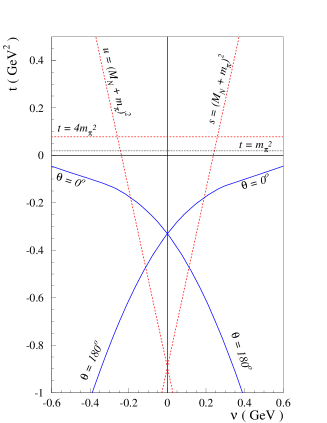
Figure 28: The Mandelstam plane for virtual Compton scattering at $Q^{2}$ = 0.33 GeV². The boundaries of the physical $s$-channel region are $\theta=0^{\mathrm{o}}$ and $\theta=180^{\mathrm{o}}$ for $\nu>0$, the $u$-channel region is obtained by crossing, $\nu\to-\nu$. The curves for $\theta=0^{\mathrm{o}}$ and $\theta=180^{\mathrm{o}}$ intersect at $\nu=0$, $t=-Q^{2}$, which is the point where the generalized polarizabilities are defined.

The VCS helicity amplitudes can be written as

$$T_{\lambda^{\prime}\lambda_{N}^{\prime};\lambda\lambda_{N}}=\,-e^{2}\varepsilon_{\mu}(q,\lambda)\,\varepsilon^{{}^{\prime}*}_{\nu}(q^{\prime},\lambda^{\prime})\,\bar{u}(p^{\prime},\lambda_{N}^{\prime})\,{\mathcal{M}}^{\mu\nu}\,u(p,\lambda_{N})\ ,$$ (223)

where the polarization four-vectors of the virtual (real) photons are denoted by $\varepsilon$ ($\varepsilon^{{}^{\prime}}$), and their helicities by $\lambda$ ($\lambda^{\prime}$), with $\lambda=0,\pm 1$ and $\lambda^{\prime}=\pm 1$. The nucleon helicities are $\lambda_{N},\lambda_{N}^{\prime}=\pm 1/2$, and $u,\bar{u}$ are the nucleon spinors. The VCS tensor ${\mathcal{M}}^{\mu\nu}$ in Eq. (223) can be decomposed into a Born (B) and a non-Born part (NB) :

$${\mathcal{M}}^{\mu\nu}\;=\;{\mathcal{M}}^{\mu\nu}_{B}\,+\,{\mathcal{M}}^{\mu\nu}_{NB}\;.$$ (224)

In the Born process, the virtual photon is absorbed on a nucleon and the intermediate state remains a nucleon, whereas the non-Born process contains all nucleon excitations and meson-loop contributions. The separation between Born and non-Born parts is performed in the same way as described in Ref. [136], to which we refer for details (see also Ref. [139]).
One can proceed by parametrizing the VCS tensor of Eq. (224) in terms of 12 independent amplitudes. In Ref. [140], a gauge-invariant tensor basis was found so that the resulting non-Born invariant amplitudes are free of kinematical singularities and constraints, which is an important property when setting up a dispersion relation formalism. This tensor takes the form

$${\mathcal{M}}^{\mu\nu}\;=\;\sum_{i=1}^{12}\;f_{i}(Q^{2},\nu,t)\,\rho^{\mu\nu}_{i}\;,$$ (225)

where the 12 independent tensors $\rho^{\mu\nu}_{i}$ are given in App. B. The corresponding 12 amplitudes $f_{i}$ are expressed in terms of the invariants $Q^{2}$, $\nu$ and $t$. The tensor basis $\rho^{\mu\nu}_{i}$ is chosen such that the resulting invariant amplitudes $f_{i}$ are either even or odd under crossing, which leads to the following symmetry relations for the $f_{i}$ at the real photon point :

$$f_{i}\left(0,\nu,t\right)\,=\,+\,f_{i}\left(0,-\nu,t\right),\hskip 5.69046pt(i=1,2,6,11)\;,$$

$$f_{i}\left(0,\nu,t\right)\,=\,-\,f_{i}\left(0,-\nu,t\right),\hskip 5.69046pt(i=4,7,9,10)\;,$$ (226)

while the amplitudes $f_{3}$, $f_{5}$, $f_{8}$, $f_{12}$ do not contribute at this point, because the corresponding tensors vanish in the limit $Q^{2}\rightarrow 0$.
Nucleon crossing combined with charge conjugation provides the more general constraints on the $f_{i}$ at arbitrary virtuality $Q^{2}$ :

$$f_{i}\left(Q^{2},\nu,t\right)\, = \,+\,f_{i}\left(Q^{2},-\nu,t\right),\hskip 2.84544pt(i=1,2,5,6,7,9,11,12),\hskip 2.84544pt$$

$$f_{i}\left(Q^{2},\nu,t\right)\, = \,-\,f_{i}\left(Q^{2},-\nu,t\right),\hskip 2.84544pt(i=3,4,8,10).\hskip 5.69046pt$$ (227)

When using dispersion relations, it will be convenient to work with 12 amplitudes that are all even in $\nu$. This is achieved by introducing the amplitudes $F_{i}$ ($i$ = 1,…,12) as follows :

$$F_{i}\left(Q^{2},\nu,t\right)\, = \,f_{i}\left(Q^{2},\nu,t\right),\hskip 5.69046pt(i=1,2,5,6,7,9,11,12)\;,$$

$$F_{i}\left(Q^{2},\nu,t\right)\, = \,{1\over\nu}\,f_{i}\left(Q^{2},\nu,t\right),\hskip 5.69046pt(i=3,4,8,10)\;,$$ (228)

satisfying $F_{i}\left(Q^{2},-\nu,t\right)=F_{i}\left(Q^{2},\nu,t\right)$ for $i$ = 1,…,12. As the non-Born invariant amplitudes $f^{NB}_{3,4,8,10}\thicksim\nu$ for $\nu\rightarrow 0$, the definition of Eq. (228) ensures that also all the non-Born amplitudes $F_{i}^{NB}$ ($i$ = 1,…,12) are free from kinematical singularities. The results for the Born amplitudes $F_{i}^{B}$ are listed in App. B of Ref. [141].
From Eqs. (226) and (227), one furthermore finds that $F_{7}$ and $F_{9}$ vanish at the real photon point. Since 4 of the tensors also vanish in the limit $Q^{2}\rightarrow 0$, only the six amplitudes $F_{1}$, $F_{2}$, $F_{4}$, $F_{6}$, $F_{10}$ and $F_{11}$ enter in real Compton scattering (RCS). These 6 amplitudes are related to the RCS amplitudes of Eq. (3.3) by

$$-e^{2}\,F_{1}\, = -A_{1}\,-\,\left({{t-4M^{2}}\over{4M^{2}}}\right)\,A_{3}\,+\,{{\nu^{2}}\over{M^{2}}}\,A_{4}\,+\,A_{6}\;,$$

$$-e^{2}\,F_{2}\, = -{1\over{2M^{2}}}\,\left[A_{3}\,+\,A_{6}\,-\,{t\over{4M^{2}}}\,A_{4}\right]\;,$$

$$-e^{2}\,F_{4}\, = {1\over{2M^{2}}}\,A_{4}\;,$$

$$-e^{2}\,F_{6}\, = {1\over{4M^{2}}}\,\left[-\left({{t-4M^{2}}\over{4M^{2}}}\right)\,A_{4}\,+\,A_{6}\right]\;,$$

$$-e^{2}\,F_{10}\, = -{1\over{2M}}\,\left[A_{5}-A_{6}\right]\;,$$

$$-e^{2}\,F_{11}\, = -{1\over 4M}\,\left[A_{2}\,-\,{{t-4M^{2}+4\nu^{2}}\over{4M^{2}}}\,A_{4}\,+\,A_{6}\right],\hskip 11.38092pt$$ (229)

where the charge factor $-e^{2}$ appears explicitly on the lhs of Eq. (229), because this factor is included in the usual definition of the $A_{i}$.

4.3 Definitions of nucleon generalized polarizabilities

The behavior of the non-Born VCS tensor ${\mathcal{M}}^{\mu\nu}_{NB}$ of Eq. (225) at low energy (${\hbox{\rm q}^{\prime}}\equiv|{\mathbf{q}}_{cm}^{\;{}^{\prime}}|\to 0$) but at arbitrary three-momentum ${\hbox{\rm q}}\,\equiv\,|{\mathbf{q}}_{cm}\,|$ of the virtual photon, can be parametrized by 6 generalized polarizabilities (GPs), which will be denoted by $P^{(\mathcal{M}^{\prime}\,L^{\prime},\,\mathcal{M}\,L)S}({\hbox{\rm q}})$ [136, 140, 142]. In this notation, $\mathcal{M}$ ($\mathcal{M}^{\prime}$) refers to the electric $(E)$, magnetic $(M)$ or longitudinal $(L)$ nature of the initial (final) photon, $L$ ($L^{\prime}$) represents the angular momentum of the initial (final) photon, and $S$ differentiates between the spin-flip ($S=1$) and non spin-flip ($S=0$) character of the transition at the nucleon side. Assuming that the emitted real photons have low energies, we may use the dipole approximation ($L^{\prime}=1$). For a dipole transition in the final state, angular momentum and parity conservation lead to 10 GPs [136]. Furthermore, it has been shown [140] that nucleon crossing combined with charge conjugation symmetry of the VCS amplitudes provide 4 additional constraints among the 10 GPS. A convenient choice for the 6 independent GPs appearing in that approximation has been proposed in Ref. [137] :

$$P^{(L1,L1)0}({\hbox{\rm q}}),\;P^{(M1,M1)0}({\hbox{\rm q}}),\;$$ (230)

$$P^{(L1,L1)1}({\hbox{\rm q}}),\;P^{(M1,M1)1}({\hbox{\rm q}}),\;P^{(M1,L2)1}({\hbox{\rm q}}),\;P^{(L1,M2)1}({\hbox{\rm q}}).\hskip 14.22636pt$$ (231)

We note at this point that the difference between the transverse electric and longitudinal transitions is of higher order in q, which explains why the electric multipoles can be replaced by the longitudinal ones in the above equations.
In the limit ${\hbox{\rm q}}\rightarrow 0$ one finds the following relations between the VCS and RCS polarizabilities [140] :

$$\begin{array}[]{lcl}P^{(L1,L1)0}(0)=-{{4\pi}\over{e^{2}}}\,\sqrt{\frac{2}{3}}\,\alpha&,&P^{(M1,M1)0}(0)=-{{4\pi}\over{e^{2}}}\,\sqrt{\frac{8}{3}}\,\beta\;,\\ P^{(L1,M2)1}(0)=-{{4\pi}\over{e^{2}}}\,\frac{\sqrt{2}}{3}\,\gamma_{3}&,&P^{(M1,L2)1}(0)=-{{4\pi}\over{e^{2}}}\,\frac{2\sqrt{2}}{3\sqrt{3}}\,\left(\gamma_{2}+\gamma_{4}\right)\;,\\ P^{(L1,L1)1}(0)=0&,&P^{(M1,M1)1}(0)=0\;.\end{array}$$

In terms of invariants, the limit ${\hbox{\rm q}^{\prime}}\to 0$ at finite three-momentum q of the virtual photon corresponds to $\nu\to 0$ and $t\to-Q^{2}$ at finite $Q^{2}$. One can therefore express the GPs in terms of the VCS invariant amplitudes $F_{i}$ at the point $\nu=0,t=-Q^{2}$ for finite $Q^{2}$, for which we introduce the shorthand :

$$\bar{F}_{i}(Q^{2})\;\equiv\;F_{i}^{NB}\left(Q^{2},\nu=0,t=-Q^{2}\right)\;.$$ (232)

The relations between the GPs and the $\bar{F}_{i}(Q^{2})$ can be found in Ref. [140].
Analogously to the sum rules which we discussed in Sec. 3 for the nucleon polarizabilities at $Q^{2}$ = 0, we now turn to dispersion relations for the GPs. From the high-energy behavior of the amplitudes $F_{i}$, it was found in Ref. [141] that the unsubtracted DRs do not exist for the amplitudes $F_{1}$ and $F_{5}$, but can be written down for the other amplitudes. Therefore, unsubtracted DRs for the GPs will hold for those GPs which do not depend on the two amplitudes $F_{1}$ and $F_{5}$. However, the amplitude $F_{5}$ can appear in the combination $F_{5}+4\,F_{11}$, because this combination has a high-energy behavior leading to a convergent integral [141, 143]. Among the six GPs we find four combinations that do not depend on $F_{1}$ and $F_{5}$ :

$$P^{\left(L1,L1\right)0} +\,{1\over 2}P^{\left(M1,M1\right)0}={{-2}\over{\sqrt{3}}}\left({{E+M}\over E}\right)^{1/2}M\tilde{q}_{0}\,\left\{{{{\hbox{\rm q}}^{2}}\over{\tilde{q}_{0}^{2}}}\,\bar{F}_{2}+\left(2\,\bar{F}_{6}+\bar{F}_{9}\right)-\bar{F}_{12}\right\},$$ (233)

$$P^{\left(L1,L1\right)1} ={1\over{3\sqrt{2}}}\,\left({{E+M}\over E}\right)^{1/2}\,\tilde{q}_{0}\,\left\{\left(\bar{F}_{5}+\bar{F}_{7}+4\,\bar{F}_{11}\right)+4\,M\,\bar{F}_{12}\right\},$$ (234)

$$P^{\left(L1,M2\right)1} -\,{1\over{\sqrt{2}\,\tilde{q}_{0}}}P^{\left(M1,M1\right)1}={1\over{3}}\left({{E+M}\over E}\right)^{1/2}{{M\,\tilde{q}_{0}}\over{{\hbox{\rm q}}^{2}}}$$

$$\times \left\{\left(\bar{F}_{5}+\bar{F}_{7}+4\,\bar{F}_{11}\right)+4\,M\left(2\,\bar{F}_{6}+\bar{F}_{9}\right)\right\},$$ (235)

$$P^{\left(L1,M2\right)1} +\,{{\sqrt{3}}\over{2}}P^{\left(M1,L2\right)1}={1\over{6}}\left({{E+M}\over E}\right)^{1/2}\,{{\tilde{q}_{0}}\over{{\hbox{\rm q}}^{2}}}$$

$$\times \left\{\tilde{q}_{0}\left(\bar{F}_{5}+\bar{F}_{7}+4\,\bar{F}_{11}\right)+8\,M^{2}\left(2\,\bar{F}_{6}+\bar{F}_{9}\right)\right\},\hskip 14.22636pt$$ (236)

where $E=\sqrt{{\hbox{\rm q}}^{2}+M^{2}}$ denotes the initial proton c.m. energy and $\tilde{q}_{0}=M-E$ the virtual photon c.m. energy in the limit ${\hbox{\rm q}^{\prime}}$ = 0. For small values of q, we observe the relation $\tilde{q}_{0}\approx-\,{\hbox{\rm q}}^{2}/(2M)$. Furthermore, in the limit ${\hbox{\rm q}^{\prime}}$ = 0, the value of $Q^{2}$ is always understood as being $\tilde{Q}^{2}\equiv{\hbox{\rm q}}^{2}-\tilde{q}_{0}^{2}$, which we denote by $Q^{2}$ for simplicity of the notation.

4.4 Fixed-$t$ dispersion relations

With the choice of the tensor basis of App. B, and taking account of the crossing relation Eq. (227), the resulting non-Born VCS invariant amplitudes $F_{i}$ ($i$ = 1,…,12) are free of kinematical singularities and constraints, and even in $\nu$, i.e., $F_{i}(Q^{2},\nu,t)\,=\,F_{i}(Q^{2},-\nu,t)$. Assuming further analyticity and an appropriate high-energy behavior, these amplitudes fulfill unsubtracted dispersion relations with respect to the variable $\nu$ at fixed $t$ and fixed virtuality $Q^{2}$,

$$\mathrm{Re}F_{i}^{NB}(Q^{2},\nu,t)\;=\;F_{i}^{pole}(Q^{2},\nu,t)\,-\,F_{i}^{B}(Q^{2},\nu,t)\,+\,{2\over\pi}\;{\mathcal{P}}\int_{\nu_{0}}^{+\infty}d\nu^{\prime}\;{{\nu^{\prime}\;\mathrm{Im}_{s}F_{i}(Q^{2},\nu^{\prime},t)}\over{\nu^{\prime 2}-\nu^{2}}}\;,$$

(237)

where we explicitly indicate that the lhs of Eq. (237) represents the non-Born ($NB$) parts of the amplitudes. In Eq. (237), $F_{i}^{B}$ is defined as in the discussion following Eq. (224), whereas $F_{i}^{pole}$ represents the nucleon pole contribution (i.e. energy factors in the numerators are evaluated at the pole position). Furthermore in Eq. (237), $\mathrm{Im}_{s}F_{i}$ are the discontinuities across the $s$-channel cuts of the VCS process, starting at the pion production threshold, which is the first inelastic channel, i.e., $\nu_{0}=m_{\pi}+(m_{\pi}^{2}+t/2+Q^{2}/2)/(2M)$.
Besides the absorptive singularities due to physical intermediate states which contribute to the rhs of dispersion integrals as Eq. (237), one might wonder if other singularities exist giving rise to imaginary parts. Such additional singularities could come from so-called anomalous thresholds [145, 146], which arise when a hadron is a loosely bound system of other hadronic constituents which can go on-shell (such as is the case of a nucleus in terms of its nucleon constituents), leading to so-called triangular singularities. It was shown that in the case of strong confinement within QCD, the quark-gluon structure of hadrons does not give rise to additional anomalous thresholds [147, 148], and the quark singularities are turned into hadron singularities described through an effective field theory. Therefore, the only anomalous thresholds arise for those hadrons which are loosely bound composite systems of other hadrons (e.g., the $\Sigma$ particle in terms of $\Lambda$ and $\pi$). For the nucleon case, such anomalous thresholds are absent, and the imaginary parts entering the dispersion integrals of Eq. (237) are calculated from absorptive singularities due to $\pi N$, $\pi\pi N$, … physical intermediate states.
The assumption that unsubtracted dispersion relations as in Eq. (237) hold, requires that at high energies ($\nu\rightarrow\infty$ at fixed $t$ and fixed $Q^{2}$) the amplitudes $\mathrm{Im}_{s}F_{i}(Q^{2},\nu,t)$ ($i$ = 1,…,12) drop fast enough so that the integrals of Eq. (237) are convergent and the contribution from the semi-circle at infinity can be neglected. The high-energy behavior of the amplitudes $F_{i}$ was investigated in [141] by considering the Regge limit ($\nu\rightarrow\infty$, at fixed $t$ and fixed $Q^{2}$) of the VCS helicity amplitudes. As mentioned above, it follows from this analysis that for the amplitudes $F_{1}$ and $F_{5}$, an unsubtracted dispersion integral does not exist, whereas the other ten VCS amplitudes can be evaluated through unsubtracted dispersion integrals as in Eq. (237).
Having specified the VCS invariant amplitudes and their high energy behavior, we are now ready to set up the DR formalism. The difference between Born and pole terms in Eq. (237) vanishes for the four combinations of GPs on the lhs of Eqs. (233 - 236). They can be directly evaluated by unsubtracted DRs through the following integrals for the corresponding $\bar{F}_{i}(Q^{2})$ :

$$\bar{F}_{i}(Q^{2})\;=\;{2\over\pi}\;\int_{\nu_{0}}^{+\infty}d\nu^{\prime}\;{{\mathrm{Im}_{s}F_{i}(Q^{2},\nu^{\prime},t=-Q^{2})}\over{\nu^{\prime}}}\;.$$ (238)

We will next discuss in Sec. 4.4.1 how the $s$-channel dispersion integrals of Eqs. (237) and (238) are evaluated. In particular, unitarity will allow us to express the imaginary parts of the VCS amplitudes in terms of $\pi N$, $\pi\pi N$,… intermediate states. Subsequently, we will show in Sec. 4.4.2 how to deal with the remaining two VCS invariant amplitudes for which one cannot write down unsubtracted DRs.

4.4.1 s-channel dispersion integrals

The imaginary parts of the amplitudes $F_{i}$ in Eq. (237) are obtained through the imaginary part of the VCS helicity amplitudes $T_{\lambda^{\prime}\lambda_{N}^{\prime};\lambda\lambda_{N}}$ defined in Eqs. (223) and (225). The VCS helicity amplitudes can be expressed by the $F_{i}$ in a straightforward manner, even though the calculation is cumbersome. The main difficulty, however, is the inversion of the relation between the two sets of amplitudes, i.e., to express the twelve amplitudes $F_{i}$ in terms of the twelve independent helicity amplitudes. This problem has been solved in Refs. [141, 149] in two different ways. Firstly, the inversion was performed numerically by applying different algorithms. Secondly, an explicit analytical inversion was found as detailed in Ref. [149]. The two different methods allow us to cross-check the results.
Having expressed the amplitudes $F_{i}$ in terms of the helicity amplitudes, the latter are determined by using unitarity. Denoting the VCS helicity amplitudes by $T_{fi}$, the unitarity relation takes the generic form

$$2\,\mathrm{Im}_{s}\,T_{fi}=\sum_{X}(2\pi)^{4}\delta^{4}(P_{X}-P_{i})T_{Xf}^{\dagger}T_{Xi}\,,$$ (239)

where the sum runs over all possible intermediate states $X$. Here we are mainly interested in VCS through the $\Delta(1232)$-resonance region. Therefore, we restrict ourselves to the dominant contribution by only taking account of the $\pi N$ $s$-channel intermediate states. If one wants to extend the dispersion formalism to higher energies, the influence of additional channels, like the $\pi\pi N$ intermediate states has to be addressed. The helicity amplitudes for $\pi N$ intermediate states are expressed in terms of pion photo- and electroproduction multipoles as specified in App. C.4 of Ref [141]. The calculations are performed by use of the phenomenological MAID analysis [18], which contains both resonant and non-resonant pion production mechanisms. This state-of-the-art analysis is based on the existing pion photo- and electroproduction data. A direct evaluation of the rhs of Eq. (239) is not possible due to an incomplete coverage of the phase space with the present data sets. Therefore, a phenomenological analysis is needed to fully calculate the dispersive input.

4.4.2 Asymptotic parts and dispersive contributions beyond $\pi N$

To evaluate the VCS amplitudes $F_{1}$ and $F_{5}$ in an unsubtracted DR framework, we proceed as in the case of RCS [75]. This amounts to perform the unsubtracted dispersion integrals of Eq. (237) for $F_{1}$ and $F_{5}$ along the real $\nu$-axis in the range $-\nu_{max}\leq\nu\leq+\nu_{max}$, and to close the contour by a semi-circle with radius $\nu_{max}$ in the upper half of the complex $\nu$-plane, with the result

$$\mathrm{Re}F_{i}^{NB}(Q^{2},\nu,t)=F_{i}^{pole}(Q^{2},\nu,t)-F_{i}^{B}(Q^{2},\nu,t)+F_{i}^{int}(Q^{2},\nu,t)+F_{i}^{as}(Q^{2},\nu,t),$$ (240)

for ($i=1,5$), where the integral contributions $F_{i}^{int}$ (for $i=1,5$) are given by

$$F_{i}^{int}(Q^{2},\nu,t)\;=\;{2\over\pi}\;{\mathcal{P}}\int_{\nu_{0}}^{\nu_{max}}d\nu^{\prime}\;{{\nu^{\prime}\;\mathrm{Im}_{s}F_{i}(Q^{2},\nu^{\prime},t)}\over{\nu^{\prime 2}-\nu^{2}}}\;,$$ (241)

and with the contributions of the semi-circle of radius $\nu_{max}$ identified with the asymptotic contributions ($F_{1}^{as}$, $F_{5}^{as}$).
Evidently, the separation between asymptotic and integral contributions in Eq. (240) is specified by the value of $\nu_{max}$. The total result for $F_{i}^{NB}$ is formally independent of the specific value of $\nu_{max}$. In practice, however, $\nu_{max}$ is chosen to be not too large so that one can evaluate the dispersive integrals of Eq. (241) from threshold up to $\nu_{max}$ sufficiently accurate. As we are mainly interested here in a description of VCS up to $\Delta(1232)$-resonance energies, the dispersion integrals are saturated by their $\pi N$ contribution and we choose $\nu_{max}=1.5$ GeV. In the following, we denote this contribution by $F_{i}^{\pi N}$. Furthermore, the remainder is estimated by an energy-independent function, which parametrizes the asymptotic contribution $F_{i}^{as}$ due to $t$-channel poles, and which contains all dispersive contributions beyond the value $\nu_{max}=1.5$ GeV. We will next discuss the asymptotic contributions $F_{5}^{as}$ and $F_{1}^{as}$.

• The asymptotic contribution $F_{5}^{as}$
  

  The asymptotic contribution to the amplitude $F_{5}$ predominantly results from the $t$-channel $\pi^{0}$-exchange  :

  $$F^{as}_{5}(Q^{2},\nu,t)\, \approx \,F_{5}^{\pi^{0}}(Q^{2},t)\,=\,-4\,F_{11}^{\pi^{0}}(Q^{2},t)\,=\,-{1\over{M}e^{2}}\,{g_{\pi NN}\;{F_{\pi^{0}\gamma\gamma}\left(Q^{2}\right)}\over{t-m_{\pi}^{2}}}\,.$$ (242)

  For the $Q^{2}$-dependence of $F_{\pi^{0}\gamma\gamma}\left(Q^{2}\right)$, one can use the interpolation formula proposed in  [150] :

  $$F_{\pi^{0}\gamma\gamma}\left(Q^{2}\right)\;=\;{F_{\pi^{0}\gamma\gamma}(0)\over{1+Q^{2}/(8\,\pi^{2}\,f_{\pi}^{2})}}\,,$$ (243)

  where $F_{\pi^{0}\gamma\gamma}(0)$ has been given in Eq. (176). Equation (243) provides a rather good parametrization of the $\pi^{0}\gamma^{*}\gamma$ form factor data over the whole $Q^{2}$ range.
  When fixing the asymptotic contribution $F_{5}^{as}$ through its $\pi^{0}$-pole contribution as in Eq. (242), one can determine one more GP of the nucleon, in addition to the 4 combinations of Eqs. (233) - (236). In particular, the GP $P^{\left(M1,M1\right)1}$ which contains $F_{5}$ can be calculated through

  $$P^{\left(M1,M1\right)1}\left(Q^{2}\right)\,= \,-{{\sqrt{2}}\over{3}}\,\left({{E+M}\over E}\right)^{1/2}{{M\,\tilde{q}_{0}^{2}}\over{{\hbox{\rm q}}^{2}}}\,\left\{\bar{F}_{5}(Q^{2})\,+\,\tilde{q}_{0}\,\bar{F}_{12}(Q^{2})\right\}.$$ (244)

  
  

• The asymptotic part and dispersive contributions beyond $\pi N$ to $F_{1}$
  

  We next turn to the high-energy contribution to $F_{1}$. As in the case of RCS, the asymptotic contribution to the amplitude $F_{1}$ originates predominantly from the $t$-channel $\pi\pi$ intermediate states. In a phenomenological analysis, this continuum is parametrized through the exchange of a scalar-isoscalar particle in the $t$-channel, i.e. an effective “$\sigma$”-meson, as suggested in [75] and discussed in Sec. 3.6 for the RCS case. In this spirit, the difference between $F_{1}^{NB}$ and its $\pi N$ contribution can be parametrized at $Q^{2}=0$ by the energy-independent function :

  $$F_{1}^{NB}(0,\nu,t)\,-\,F_{1}^{\pi N}(0,\nu,t)\,\approx\,\left[F_{1}^{NB}(0,0,0)-F_{1}^{\pi N}(0,0,0)\right]\,{{1}\over{1-t/m_{\sigma}^{2}}}\;,$$ (245)

  where $F_{1}^{\pi N}$ is evaluated through a dispersive integral as discussed in Eq. (238), and the $\sigma$-meson mass $m_{\sigma}$ is a free parameter as in the fixed-$t$ unsubtracted RCS dispersion analysis. A fit to the $t$-dependence of RCS data results in $m_{\sigma}\approx$ 0.6 GeV [75]. The value $F_{1}^{NB}(0,0,0)$ is then considered as a remaining global fit parameter to be extracted from experiment. It can be expressed physically in terms of the magnetic dipole polarizability $\beta$ :

  $$F_{1}^{NB}(0,0,0)\,=\,{{4\pi}\over{e^{2}}}\;\beta\;.$$ (246)

  The term $F_{1}^{\pi N}(0,0,0)$ in Eq. (245), can be calculated through a dispersion integral and results in the value :

  $$\alpha_{em}\,F_{1}^{\pi N}(0,0,0)\,=\,\beta^{\pi N}\,=\,9.1\;,$$ (247)

  in units of $10^{-4}$ fm³. From the $\pi N$ contribution $\beta^{\pi N}$ of Eq. (247), and the phenomenological value $\beta$ of Eq. (3.4), one obtains the difference

  $$\beta-\beta^{\pi N}=-7.5\;,$$ (248)

  which enters in the rhs of Eq. (245). As discussed before, the small total value of the magnetic polarizability $\beta$ comes about by a near cancellation between a large (positive) paramagnetic contribution ($\beta^{\pi N}$) and a large (negative) diamagnetic contribution ($\beta-\beta^{\pi N}$), i.e., the asymptotic part of $F_{1}$ parametrizes the diamagnetism.
  Turning next to the $Q^{2}$ dependence of the asymptotic contribution to $F_{1}$, it has been proposed in [141] to parametrize this part of the non-Born term $F_{1}^{NB}(Q^{2},\nu,t)$ beyond its $\pi N$ dispersive contribution, by an energy independent $t$-channel pole of the form :

  $$F_{1}^{NB}(Q^{2},\nu,t)\,-\,F_{1}^{\pi N}(Q^{2},\nu,t)\,\approx\,{{f(Q^{2})}\over{1-t/m_{\sigma}^{2}}}\;.$$ (249)

  The function $f(Q^{2})$ in Eq. (249) can be obtained by evaluating the $lhs$ of Eq. (249) at the point where the GPs are defined, i.e., $\nu=0$ and $t=-Q^{2}$, at finite $Q^{2}$. This leads to :

  $$f(Q^{2})\,=\,\left[\bar{F}_{1}(Q^{2})-\bar{F}_{1}^{\pi N}(Q^{2})\right]\;\left(1+Q^{2}/m_{\sigma}^{2}\right)\;,$$ (250)

  where the shorthand $\bar{F}_{1}(Q^{2})$ is defined in Eq. (232). Equations (249) and (250) then lead to the following expression for the VCS amplitude $F_{1}^{NB}$ :

  $$F_{1}^{NB}(Q^{2},\nu,t) \approx F_{1}^{\pi N}(Q^{2},\nu,t)\,+\,\left[\bar{F}_{1}(Q^{2})\,-\,\bar{F}_{1}^{\pi N}(Q^{2})\right]\,{{1+Q^{2}/m_{\sigma}^{2}}\over{1-t/m_{\sigma}^{2}}},\hskip 5.69046pt$$ (251)

  where the $\pi N$ contributions $F_{1}^{\pi N}(Q^{2},\nu,t)$ and $\bar{F}_{1}^{\pi N}(Q^{2})$ are calculated through dispersion integrals as given by Eqs. (238) and (241) respectively. Consequently, the only unknown quantity on the rhs of Eq. (251) is $\bar{F}_{1}(Q^{2})$, which can be directly used as a fit parameter at finite $Q^{2}$. The quantity $\bar{F}_{1}(Q^{2})$ can be expressed in terms of the generalized magnetic polarizability $P^{(M1,M1)0}$ of Eq. (230) as [140] :

  $$\bar{F}_{1}(Q^{2})\, = \,-\sqrt{{3\over 8}}\,\left({{2E}\over{E+M}}\right)^{1/2}\,P^{\left(M1,M1\right)0}(Q^{2})\,\equiv\,{{4\pi}\over{e^{2}}}\,\left({{2E}\over{E+M}}\right)^{1/2}\,\beta(Q^{2})\,,$$ (252)

  where $\beta(Q^{2}$) is the generalized magnetic polarizability, which reduces to the polarizability $\beta$ of RCS at $Q^{2}$ = 0. The parametrization of Eq. (251) for $F_{1}$ then permits to directly extract $\beta(Q^{2})$ from VCS observables at a fixed $Q^{2}$. In the following, we consider a convenient parametrization of the $Q^{2}$ dependence of $\beta(Q^{2})$ in order to provide predictions for VCS observables. For this purpose it was proposed in [141] to use a dipole parametrization for the difference $\beta(Q^{2})-\beta^{\pi N}(Q^{2})$, which enters in the rhs of Eq. (251) via Eq. (252), as  :

  $$\beta(Q^{2})-\beta^{\pi N}(Q^{2})\,=\,{{\left(\beta-\beta^{\pi N}\right)}\over{\left(1+Q^{2}/\Lambda^{2}_{\beta}\right)^{2}}}\,,$$ (253)

  where the RCS value $(\beta-\beta^{\pi N})$ on the rhs is given by Eq. (248). The mass scale $\Lambda_{\beta}$ in Eq. (253) determines the $Q^{2}$ dependence, and hence gives us the information how the diamagnetism is spatially distributed in the nucleon. Using the dipole parametrization of Eq. (253), one can extract $\Lambda_{\beta}$ from a fit to VCS data at different $Q^{2}$ values, and check the parametrization of Eq. (253) for the asymptotic contribution to $\beta(Q^{2})$.
  To have some educated guess on the physical value of $\Lambda_{\beta}$, we next discuss two microscopic calculations of the diamagnetic contribution to the GP $\beta(Q^{2})$. The diamagnetism of the nucleon is dominated by the pion cloud surrounding the nucleon. This diamagnetic contribution has been estimated in Ref. [141] through a DR calculation of the $t$-channel $\pi\pi$ intermediate state contribution to $F_{1}$. Such a dispersive estimate has been discussed before for RCS in Sec. 3.7, where it was shown that the asymptotic part of $F_{1}$ (or equivalently $A_{1}$) can be related to the $\gamma\gamma\to\pi\pi\to N\bar{N}$ process. The dominant contribution is due to the $\pi\pi$ intermediate state with spin and isospin zero ($I=J=0$). The generalization to VCS leads then to the identification of $F_{1}^{as}$ with the following unsubtracted DR in $t$ at fixed energy $\nu=0$ :

  $$\bar{F}_{1}^{as}(Q^{2})\,=\,\frac{1}{\pi}\int^{\infty}_{4m_{\pi}^{2}}dt^{\prime}\,\frac{\mathrm{Im}_{t}F_{1}(Q^{2},0,t^{\prime})}{t^{\prime}+Q^{2}}\,.$$ (254)

  The imaginary part on the rhs of Eq. (254) has been evaluated in Ref. [141] through the subprocesses $\gamma^{*}\gamma\rightarrow\pi\pi$ and $\pi\pi\rightarrow N{\bar{N}}$. To describe the $Q^{2}$ dependence of the $\gamma^{*}\gamma\rightarrow\pi\pi$ amplitude, which is dominated by the unitarized Born amplitude (on the pion), the pion electromagnetic form factor was included. The result for this dispersive estimate of $\bar{F}_{1}^{as}$ through $t$-channel $\pi\pi$ intermediate states is shown in Fig. 29, and compared with the corresponding evaluation of Ref. [151] in the linear $\sigma$-model (LSM). The LSM calculation overestimates the value of $\bar{F}_{1}^{as}(0)$ (or equivalently $\beta_{as}$) by about 30% at any realistic value of $m_{\sigma}$, which is a free parameter in this calculation. However, as for the dispersive calculation, it also shows a steep $Q^{2}$ dependence.

  

  Figure 29: Theoretical estimates of the asymptotic contribution $F_{1}^{as}$ : DR calculation [141] of the $\gamma^{*}\gamma\to\pi\pi\to N\bar{N}$ process (solid curve); linear $\sigma$-model (LSM) calculation [151] with $m_{\sigma}$ = 0.5 GeV (dotted curve) and $m_{\sigma}$ = 0.7 GeV (dashed-dotted curve). The dashed curves are dipole parametrizations according to Eq. (253), which are fixed to the phenomenological value at $Q^{2}$ = 0 and are shown for two values of the mass-scale, $\Lambda_{\beta}$ = 0.4 GeV (upper dashed curve, nearly coinciding with solid curve) and $\Lambda_{\beta}$ = 0.6 GeV (lower dashed curve).

  Furthermore in Fig. 29, the two model calculations discussed above are compared with the dipole parametrization of Eq. (253) for the two values $\Lambda_{\beta}$ = 0.4 GeV and $\Lambda_{\beta}$ = 0.6 GeV. It is seen that these values are compatible with the microscopic estimates discussed before. In particular, the result for $\Lambda_{\beta}$ = 0.4 GeV is nearly equivalent to the dispersive estimate of $\pi\pi$ exchange in the $t$-channel. The value of the mass scale $\Lambda_{\beta}$ is small compared to the typical scale of $\Lambda_{D}\approx$ 0.84 GeV appearing in the nucleon magnetic (dipole) form factor. This reflects the fact that diamagnetism has its physical origin in the pionic degrees of freedom, i.e., the diamagnetism is situated in the surface and intermediate region of the nucleon.
  

• Dispersive contributions beyond $\pi N$ to $F_{2}$
  

  Though we can write down unsubtracted DRs for all invariant amplitudes (or combinations of invariant amplitudes) except for $F_{1}$ and $F_{5}$, one might wonder about the quality of our approximation to saturate the unsubtracted dispersion integrals by $\pi N$ intermediate states only. This question is particularly relevant for the amplitude $F_{2}$, for which we next investigate the size of dispersive contributions beyond the $\pi N$ channel. We start with the case of RCS, where one can quantify the higher dispersive corrections to $F_{2}$, because the value of $F_{2}^{NB}$ at the real photon point can be expressed exactly (see Eqs. (4.3) and (233)) in terms of the scalar polarizability $(\alpha+\beta)$ as

  $$F_{2}^{NB}(0,0,0)\,=\,-{{4\pi}\over{e^{2}}}\,{1\over{(2M)^{2}}}\,\left(\alpha+\beta\right)\,.$$ (255)

  The $\pi N$ dispersive contribution provides the value

  $$(\alpha+\beta)^{\pi N}=11.6\,,$$ (256)

  which falls short by about 15 % compared to the Baldin’s sum rule value of Eq. (2.2). The remaining part originates from higher dispersive contributions ($\pi\pi N$, …) to $F_{2}$. These higher dispersive contributions could be calculated through unitarity, by use of Eq. (239), similarly to the $\pi N$ contribution. However, the present data for the production of those intermediate states (e.g., $\gamma^{*}N\to\pi\pi N$) are still too scarce to evaluate the imaginary parts of the VCS amplitude $F_{2}$ directly. Therefore, we estimate the dispersive contributions beyond $\pi N$ by an energy-independent constant, which is fixed to its phenomenological value at $\nu=t=0$. This yields at $Q^{2}=0$ :

  $$F_{2}^{NB}(0,\nu,t) \approx F_{2}^{\pi N}(0,\nu,t)\,-\,{{4\pi}\over{e^{2}}}\,{1\over{(2M)^{2}}}\,\left[\,\left(\alpha+\beta\right)\,-\,\left(\alpha+\beta\right)^{\pi N}\,\right],\hskip 5.69046pt$$ (257)

  which is an exact relation at $\nu=t=0$, the point where the polarizabilities are defined.
  The approximation of Eq. (257) to replace the dispersive contributions beyond $\pi N$ by a constant can only be valid if one stays below the thresholds for those higher contributions. Since the next threshold beyond $\pi N$ is $\pi\pi N$, the approximation of Eq. (257) restricts us in practice to energies below the $\Delta(1232)$-resonance.
  We next consider the extension to VCS, and focus our efforts to describe VCS into the $\Delta(1232)$-resonance region. Analogously to Eq. (257) for RCS, the dispersive contributions beyond $\pi N$ are approximated by an energy-independent constant. This constant is fixed at arbitrary $Q^{2}$, $\nu=0$, and $t=-Q^{2}$, which is the point where the GPs are defined. One thus obtains for $F_{2}^{NB}$ [141] :

  $$F_{2}^{NB}(Q^{2},\nu,t)\approx F_{2}^{\pi N}(Q^{2},\nu,t)\;+\;\left[\bar{F}_{2}(Q^{2})\,-\,\bar{F}_{2}^{\pi N}(Q^{2})\right]\,,$$ (258)

  where $\bar{F}_{2}(Q^{2})$ is defined as in Eq. (232), and can be expressed in terms of GPs through relations as given by Eqs. (233) - (236). We saturate the 3 combinations of spin GPs in Eqs. (234) - (236) by their $\pi N$ contribution, and include for the fourth spin GP of Eq. (244) also the $\pi^{0}$-pole contribution. Therefore, we only consider dispersive contributions beyond the $\pi N$ intermediate states for the two scalar GPs, which are therefore the two fit quantities in the present DR formalism for VCS. In this way, one can use Eq. (233), to write the difference $\bar{F}_{2}(Q^{2})-\bar{F}_{2}^{\pi N}(Q^{2})$ entering in the rhs of Eq. (258) as :

  $$\bar{F}_{2}(Q^{2})-\bar{F}_{2}^{\pi N}(Q^{2})\, \approx\,{{4\pi}\over{e^{2}}}\,\left({{2E}\over{E+M}}\right)^{1/2}\,{{\tilde{q}_{0}}\over{{\hbox{\rm q}}^{2}}}\,{1\over{2M}}$$ (259)

  $$\times\left\{\;\left[\alpha(Q^{2})\,-\,\alpha^{\pi N}(Q^{2})\right]\,+\,\left[\beta(Q^{2})\,-\,\beta^{\pi N}(Q^{2})\right]\;\right\},$$

  in terms of the generalized magnetic polarizability $\beta(Q^{2})$ of Eq. (252), and the generalized electric polarizability $\alpha(Q^{2}$), which is related to the GP $P^{(L1,L1)0}(Q^{2})$ by Eq. (4.3).
  We stress that Eqs. (251) and (259) are intended to extract the two GPs $\alpha(Q^{2})$ and $\beta(Q^{2})$ from VCS observables minimizing the model dependence as much as possible. As discussed before for $\beta(Q^{2})$, we next consider a convenient parametrization of the $Q^{2}$ dependence of $\alpha(Q^{2})$ in order to provide predictions for VCS observables. For this purpose, a dipole form has been proposed in Ref. [141] for the difference $\alpha(Q^{2})-\alpha^{\pi N}(Q^{2})$ which enters in the rhs of Eq. (259),

  $$\alpha(Q^{2})-\alpha^{\pi N}(Q^{2})\,=\,{{\left(\alpha-\alpha^{\pi N}\right)}\over{\left(1+Q^{2}/\Lambda^{2}_{\alpha}\right)^{2}}}\,,$$ (260)

  where the $Q^{2}$ dependence is governed by the mass scale $\Lambda_{\alpha}$, the second free parameter of the DR formalism. In Eq. (260), the RCS value

  $$(\alpha-\alpha^{\pi N})\,=\,9.6\,,$$ (261)

  is obtained from the phenomenological value of Eq. (3.4) for $\alpha$, and from the calculated $\pi N$ contribution, $\alpha^{\pi N}$ = 2.5. Using the dipole parametrization of Eq. (260), one can extract the free parameter $\Lambda_{\alpha}$ from a fit to VCS data at different $Q^{2}$ values.

4.5 VCS data for the proton and extraction of generalized polarizabilities

Having set up the dispersion formalism for VCS, we now show the predictions for the different $ep\to ep\gamma$ observables for energies up to the $\Delta(1232)$-resonance region. The aim of the experiments is to extract the 6 GPs of Eqs. (230) and (231) from both unpolarized and polarized observables. We will compare the DR results, which take account of the full dependence of the $ep\to ep\gamma$ observables on the energy (${\hbox{\rm q}^{\prime}}$) of the emitted photon, with a low-energy expansion (LEX) in ${\hbox{\rm q}^{\prime}}$. In the LEX of observables, only the first three terms of a Taylor expansion in ${\hbox{\rm q}^{\prime}}$ are taken into account. In such an expansion in ${\hbox{\rm q}^{\prime}}$, the experimentally extracted VCS unpolarized squared amplitude ${\mathcal{M}}^{\rm exp}$ takes the form [136] :

$${\mathcal{M}}^{\rm exp}=\frac{{\mathcal{M}}^{\rm exp}_{-2}}{{\hbox{\rm q}^{\prime}}^{2}}+\frac{{\mathcal{M}}^{\rm exp}_{-1}}{{\hbox{\rm q}^{\prime}}}+{\mathcal{M}}^{\rm exp}_{0}+O({\hbox{\rm q}^{\prime}})\,.$$ (262)

Due to the low energy theorem (LET), the threshold coefficients ${\mathcal{M}}^{\rm exp}_{-2}$ and ${\mathcal{M}}^{\rm exp}_{-1}$ are known [136], and are fully determined from the Bethe-Heitler + Born (BH + B) amplitudes. The information on the GPs is contained in ${\mathcal{M}}^{\rm exp}_{0}$, which contains a part originating from the BH+B amplitudes and another one which is a linear combination of the GPs, with coefficients determined by the kinematics. The unpolarized observable ${\mathcal{M}}^{\rm exp}_{0}$ can be expressed in terms of 3 structure functions $P_{LL}({\hbox{\rm q}})$, $P_{TT}({\hbox{\rm q}})$, and $P_{LT}({\hbox{\rm q}})$ by  [136] :

$${\mathcal{M}}^{\rm exp}_{0}-{\mathcal{M}}^{\rm BH+B}_{0}=2K_{2}\Bigg{\{}v_{1}\left[{\varepsilon P_{LL}({\hbox{\rm q}})-P_{TT}}({\hbox{\rm q}})\right]+\left(v_{2}-\frac{\tilde{q}_{0}}{{\hbox{\rm q}}}v_{3}\right)\sqrt{2\varepsilon\left({1+\varepsilon}\right)}P_{LT}({\hbox{\rm q}})\Bigg{\}},$$ (263)

where $K_{2}$ is a kinematical factor, $\varepsilon$ is the virtual photon polarization (in the standard notation used in electron scattering), and $v_{1},v_{2},v_{3}$ are kinematical quantities depending on $\varepsilon$ and q as well as on the cm polar and azimuthal angles ($\theta^{\gamma*\gamma}_{{\rm cm}}$ and $\phi$, respectively) of the produced real photon (for details see Ref. [137]). The 3 unpolarized observables of Eq. (263) can be expressed in terms of the 6 GPs as [136, 137] :

$$P_{LL}\,=\,-2\sqrt{6}\,M\,G_{E}\,P^{\left({L1,L1}\right)0}\;,$$ (264)

$$P_{TT}\,=\,-3\,G_{M}\,\frac{{\hbox{\rm q}}^{2}}{\tilde{q}_{0}}\left(P^{(M1,M1)1}\,-\,\sqrt{2}\,\tilde{q}_{0}\,P^{(L1,M2)1}\right),$$ (265)

$$P_{LT}\,=\,\sqrt{\frac{3}{2}}\,\frac{M\,{\hbox{\rm q}}}{Q}\,G_{E}\,P^{(M1,M1)0}\,+\,\frac{3}{2}\,\frac{Q\,{\hbox{\rm q}}}{\tilde{q}_{0}}\,G_{M}\,P^{(L1,L1)1},\hskip 17.07182pt$$ (266)

where $G_{E}$ and $G_{M}$ stand for the electric and magnetic nucleon form factors $G_{E}(Q^{2})$ and $G_{M}(Q^{2})$, respectively.
The first VCS experiment was performed at MAMI [131] and the response functions $P_{LT}$ and $P_{LL}$ - $P_{TT}/\varepsilon$ were extracted at $Q^{2}$ = 0.33 GeV² by performing a LEX to these VCS data, according to Eq. (263). To test the validity of such a LEX, we show in Fig. 30 the DR predictions for the full energy dependence of the non-Born part of the $ep\to ep\gamma$ cross section in the kinematics of the MAMI experiment [131]. This energy dependence is compared with the LEX, which predicts a linear dependence in ${\hbox{\rm q}^{\prime}}$ for the difference between the experimentally measured cross section and its BH + B contribution. The result of a best fit to the data in the framework of the LEX is indicated by the horizontal bands in Fig. 30 for the quantity $(d^{5}\sigma-d^{5}\sigma^{{\rm BH+Born}})/\Phi{\hbox{\rm q}^{\prime}}$, where $\Phi$ is a phase space factor defined in Ref. [136]. The fivefold differential cross section $d^{5}\sigma$ is differential with respect to the electron lab energy and lab angles and the proton c.m. angles, and stands in all of the following for $d\sigma\,/\,dk^{e}_{lab}\,d\Omega^{e}_{lab}\,d\Omega^{p}_{c.m.}$. It is seen from Fig. 30 that the DR results predict only a modest additional energy dependence up to ${\hbox{\rm q}^{\prime}}\simeq$ 0.1 GeV and for most of the photon angles involved, and therefore support the LEX analysis of [131]. Only for forward angles, $\theta^{\gamma*\gamma}_{{\rm cm}}\approx 0$, which is the angular range from which the value of $P_{LT}$ is extracted, the DR calculation predicts a stronger energy dependence in the range up to ${\hbox{\rm q}^{\prime}}\simeq$ 0.1 GeV, as compared to the LEX.

Figure 30: $(d^{5}\sigma-d^{5}\sigma^{{\rm BH+Born}})/\Phi{\hbox{\rm q}^{\prime}}$ for the $ep\to ep\gamma$ reaction as function of the outgoing-photon energy ${\hbox{\rm q}^{\prime}}$ in MAMI kinematics : $\varepsilon=0.62$, ${\hbox{\rm q}}=0.6$ GeV, $\phi=0^{\mathrm{o}}$, and for different photon c.m. angles $\theta^{\gamma*\gamma}_{{\rm cm}}$. The data and the shaded bands, representing the best fit to the data within the LEX formalism, are from [131]. The solid curves are the DR results taking into account the full ${\hbox{\rm q}^{\prime}}$ dependence of the non-Born contribution to the cross section. The asymptotic contributions are calculated according to Eqs. (253) and (260), with $\Lambda_{\beta}=0.6$ GeV and $\Lambda_{\alpha}=1$ GeV, respectively.

In Fig. 31, we display the response functions $P_{LL}-P_{TT}/\varepsilon$ and $P_{LT}$ at $Q^{2}$ = 0.33 GeV², which have been extracted from the cross section data of Fig. 30 [131], and compare them with the corresponding DR calculations. For the electromagnetic form factors in Eqs. (264)-(266) we use the Höhler parametrization [152] as in the analysis of the MAMI experiment [131]. In the lower panel of Fig. 31, the $Q^{2}$-dependence of the VCS response function $P_{LT}$ is displayed, which reduces to the magnetic polarizability $\beta$ at the real photon point. At finite $Q^{2}$, it contains both the scalar GP $\beta(Q^{2})$ and the spin GP $P^{(L1,L1)1}$, as seen from Eq. (266). It is obvious from Fig. 31 that the structure function $P_{LT}$ results from a large dispersive $\pi N$ (paramagnetic) contribution, which is dominated by $\Delta(1232)$ resonance excitation, and a large asymptotic (diamagnetic) contribution to $\beta$ with opposite sign, leading to a relatively small net result. The asymptotic contribution is shown in Fig. 31 with the parametrization of Eq. (253) for the values $\Lambda_{\beta}$ = 0.4 and $\Lambda_{\beta}$ = 0.6 GeV, which were also displayed in Fig. 29. Due to the large cancellation in $P_{LT}$, its $Q^{2}$ dependence is a very sensitive observable to study the interplay of the two mechanisms. In particular, one expects a faster fall-off of the asymptotic contribution with $Q^{2}$ in comparison to the $\pi N$ dispersive contribution, as discussed before. This is highlighted by the measured value of $P_{LT}$ at $Q^{2}$ = 0.33 GeV² [131], which is comparable to the value of $P_{LT}$ at $Q^{2}$ = 0. As seen from Fig. 31, this points to an interesting structure in the $Q^{2}$ region around 0.05 - 0.1 GeV², where forthcoming data are expected from an experiment at MIT-Bates [133].
In the upper panel of Fig. 31, we show the $Q^{2}$-dependence of the VCS response function $P_{LL}$ - $P_{TT}/\varepsilon$, which reduces at the real photon point to the electric polarizability $\alpha$. At non-zero $Q^{2}$, $P_{LL}$ is directly proportional to the scalar GP $\alpha(Q^{2})$, as seen from Eq. (264), and the response function $P_{TT}$ of Eq. (265) contains only spin GPs. As is shown by Fig. 31, the $\pi N$ dispersive contribution to $\alpha$ and to the spin GPs in $P_{TT}$ are smaller than the asymptotic contribution to $\alpha$. At $Q^{2}$ = 0, the $\pi N$ dispersive and asymptotic contributions to $\alpha$ have the same sign and lead to a large value of $\alpha$, in contrast to $\beta$ where both contributions have opposite sign and largely cancel each other in their sum.

Figure 31: Results for the unpolarized structure functions $P_{LL}-P_{TT}/\varepsilon$ (upper panels), and $P_{LT}$ (lower panels), for $\varepsilon$ = 0.62. Upper left panel : dispersive $\pi N$ contribution of the GP $\alpha$ (solid curve, S0), dispersive $\pi N$ contribution of the spin-flip GPs (dashed curve, S1), and the asymptotic contribution (AS) of $\alpha$ according to Eq. (260) with $\Lambda_{\alpha}=1$ GeV (dotted curve). Upper right panel : total result for $P_{LL}-P_{TT}/\varepsilon$ (sum of the three contributions on the upper left panel) for $\Lambda_{\alpha}=1$ GeV (solid curve) and $\Lambda_{\alpha}=1.4$ GeV (dashed curve). Lower left panel : dispersive $\pi N$ contribution of the GP $\beta$ (solid curve, S0), contribution of the spin-flip GPs (dashed curve, S1), and the asymptotic contribution (AS) of $\beta$ according to Eq. (253) with $\Lambda_{\beta}=0.6$ GeV (dotted curve). Lower right panel : total result for $P_{LT}$, for $\Lambda_{\beta}=0.7$ GeV (dotted curve), $\Lambda_{\beta}=0.6$ GeV (solid curve), and $\Lambda_{\beta}=0.4$ GeV (dashed curve). The RCS data are from Ref. [87], and the VCS data at $Q^{2}=0.33\mbox{\, GeV}^{2}$ from Ref. [131].

Increasing the energy, we show in Fig. 32 the DR predictions for photon energies in the $\Delta(1232)$-resonance region. It is seen that the $ep\to ep\gamma$ cross section rises strongly when crossing the pion threshold. In the dispersion relation formalism, which is based on unitarity and analyticity, the rise of the cross section with ${\hbox{\rm q}^{\prime}}$ below pion threshold, due to virtual $\pi N$ intermediate states, is connected to the strong rise of the cross section with ${\hbox{\rm q}^{\prime}}$ when a real $\pi N$ intermediate state can be produced. It is furthermore seen from Fig. 32 (lower panel) that the region between pion threshold and the $\Delta$-resonance peak displays an enhanced sensitivity to the GPs through the interference with the rising Compton amplitude due to $\Delta$-resonance excitation. For example, at ${\hbox{\rm q}^{\prime}}\simeq$ 0.2 GeV, the predictions for $P_{LT}$ in the lower right panel of Fig. 31 for $\Lambda_{\beta}$ = 0.4 GeV and $\Lambda_{\beta}$ = 0.6 GeV give a difference of about 20 % in the non-Born squared amplitude. In contrast, the LEX prescription results in a relative effect for the same two values of $P_{LT}$ of about 10% or less. This is similar to the situation discussed in Sec. 3.4 for RCS, where the region between pion threshold and the $\Delta$-resonance position also provides an enhanced sensitivity to the polarizabilities and is used to extract those polarizabilities from data using a DR formalism. Therefore, the energy region between pion threshold and the $\Delta$-resonance seems promising to measure VCS observables with an increased sensitivity to the GPs. Such an experiment has been proposed at MAMI and is underway [134].

Figure 32: Upper panel: The differential cross section for the reaction $ep\to ep\gamma$ as function of the outgoing-photon energy ${\hbox{\rm q}^{\prime}}$ in MAMI kinematics : $\varepsilon=0.62$, ${\hbox{\rm q}}=0.6$ GeV, and for $\theta^{\gamma*\gamma}_{{\rm cm}}=0^{\rm o}$, in plane ($\phi=0^{\rm o}$). The BH + B contribution is given by the dashed-dotted curve. Lower panel: Results for $(d^{5}\sigma-d^{5}\sigma^{{\rm BH+Born}})/\Phi{\hbox{\rm q}^{\prime}}$ as function of ${\hbox{\rm q}^{\prime}}$ . The total DR results are obtained with the asymptotic parts of Eqs. (253) and (260), using a fixed value of $\Lambda_{\alpha}=1$ GeV and for the same three values of $\Lambda_{\beta}$ as displayed in the lower right plot of Fig. 31, i.e. $\Lambda_{\beta}=0.7$ GeV (dotted curve), $\Lambda_{\beta}=0.6$ GeV (solid curve), and $\Lambda_{\beta}=0.4$ GeV (dashed curve). In the lower panel, the DR calculations taking into account the full energy dependence of the non-Born contribution (thick curves) are compared to the corresponding results within the LEX formalism (thin horizontal curves). The data are from Ref. [131].

When crossing the pion threshold, the VCS amplitude acquires an imaginary part due to the coupling to the $\pi N$ channel. Therefore, single polarization observables become non-zero above pion threshold. A particularly relevant observable is the electron single spin asymmetry (SSA), which is obtained by flipping the electron beam helicity [137]. For VCS, this observable is mainly due to the interference of the real BH + B amplitude with the imaginary part of the VCS amplitude. As the SSA vanishes in-plane, its measurement requires an out-of-plane experiment. Such experiments have been proposed both at MAMI [134] and at MIT-Bates [153]. In Fig. 33, the SSA is shown for a kinematics in the $\Delta(1232)$ region, corresponding with $W\approx 1.2$ GeV. The DR calculation firstly shows that the SSA is quite sizable in the $\Delta(1232)$ region. The SSA, which is mainly sensitive to the imaginary part of the VCS amplitude, displays only a rather weak dependence on the magnetic GPs $\beta(Q^{2})$, and shows a modest dependence on $\alpha(Q^{2})$. Therefore, it provides an excellent cross-check of the dispersive input in the DR formalism for VCS, in particular by comparing at the same time the pion and photon electroproduction channels through the $\Delta$ region.

Figure 33: Electron single spin asymmetry (SSA) for VCS in MAMI kinematics as function of the photon scattering angle. The full dispersion results are shown for the values: $\Lambda_{\alpha}=1$ GeV, $\Lambda_{\beta}=0.6$ GeV (solid curve), $\Lambda_{\alpha}=1$ GeV, $\Lambda_{\beta}=0.4$ GeV (dashed curve), $\Lambda_{\alpha}=1$ GeV, $\Lambda_{\beta}=0.7$ GeV (dotted curve), and $\Lambda_{\alpha}=1.4$ GeV, $\Lambda_{\beta}=0.4$ GeV (dashed-dotted curve).

Going to higher $Q^{2}$, the VCS process has also been measured at JLab and data have been obtained both below pion threshold at $Q^{2}$ = 1 GeV² [154], at $Q^{2}$ = 1.9 GeV² [155], as well as in the resonance region around $Q^{2}$ = 1 GeV² [156] (see Ref. [132] for a short review of these JLab data).
In Fig. 34, we show the results for the $ep\to ep\gamma$ reaction in the resonance region at $Q^{2}=1$ GeV² and at a backward angle. These are the first VCS measurements ever performed in the resonance region. We also display the DR calculations of [141] for the cross section. The data clearly show the excitation of the $\Delta(1232)$ resonance, and display a second and third resonance region, mainly due to the excitations of the $D_{13}(1520)$ and $F_{15}(1680)$ resonances. The DR calculations reproduce well the $\Delta(1232)$ region. Due to scarce information for the dispersive input above the $\Delta(1232)$ resonance, the DR calculations cannot be extended at present into the second and third resonance regions. Between pion threshold and the $\Delta(1232)$ resonance, the calculations show a sizable sensitivity to the GPs, in particular to $P_{LL}$ in this backward angle kinematics, and seem very promising to extract information on the electric polarizability. The precise extraction of GPs from VCS data at these higher values of $Q^{2}$, requires an accurate knowledge of the nucleon electromagnetic form factors (FFs) in this region. For the proton electromagnetic form factors, we use the new empirical fit of [157], which includes the recent high accuracy measurements performed at JLab for the ratio of proton electric FF $G_{E}$ to the magnetic FF $G_{M}$ in the $Q^{2}$ range 0.4 - 5.6 GeV² [70, 71]. From Fig. 34, one sees that a good description of the JLab data is obtained by the values $\Lambda_{\alpha}=1.0$ GeV and $\Lambda_{\beta}=0.45$ GeV.

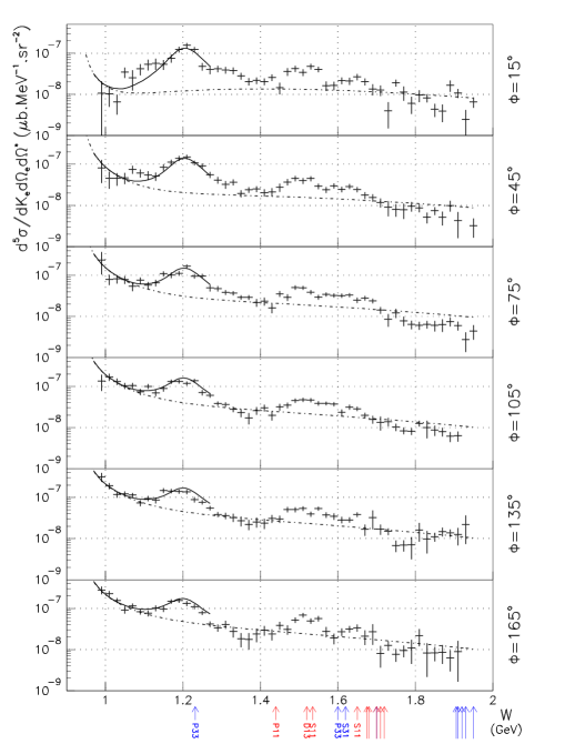
Figure 34: The differential cross sections for the $ep\to ep\gamma$ reaction as function of the c.m. energy W in JLab kinematics : $E_{e}$ = 4.032 GeV, $Q^{2}=1.0$ GeV², and for fixed scattering angle $\theta^{\gamma*\gamma}_{\rm cm}=-167.2^{\rm o}$, for different out-of-plane angles $\phi$. The BH + B contribution is given by the dashed curve. The total DR result is shown by the solid curve (limited to W $<$ 1.25 GeV) for the values $\Lambda_{\alpha}=1.0$ GeV and $\Lambda_{\beta}=0.45$ GeV. The data are from Ref. [132].

Besides the measurement in the resonance region, the $ep\to ep\gamma$ reaction has also been measured at JLab below pion threshold for three values of the outgoing photon energy at $Q^{2}$ = 1 GeV² [154], and at $Q^{2}$ = 1.9 GeV² [155]. For those kinematics, we show in Fig. 35 the differential cross sections as well as the non-Born effect relative to the BH + B cross section. It is seen from Fig. 35 that the sensitivity to the GPs is largest where the BH + B cross section becomes small, in particular in the angular region between 0^o and 50^o. In Fig. 35, we show the non-Born effect for different values of the GPs.

Figure 35: The differential cross section for the reaction $ep\to ep\gamma$ as function of the photon scattering angle, at different values of the outgoing-photon energy in JLab kinematics: $Q^{2}=1$ GeV² and $\varepsilon=0.95$ (left panels) and $Q^{2}=1.9$ GeV² and $\varepsilon=0.88$ (right panels). The BH + B cross sections are shown by the dashed-dotted curves. The DR results are displayed with the asymptotic terms parametrized as in Eqs. (260) and (253), using the values : $\Lambda_{\alpha}$ = 1 GeV and $\Lambda_{\beta}$ = 0.6 GeV (solid curves), $\Lambda_{\alpha}$ = 1 GeV and $\Lambda_{\beta}$ = 0.4 GeV (dashed curves), $\Lambda_{\alpha}$ = 1.4 GeV and $\Lambda_{\beta}$ = 0.6 GeV (dotted curves).

From the JLab data below pion threshold, the two unpolarized structure functions $P_{LL}-P_{TT}/\varepsilon$ and $P_{LT}$ have been extracted at $Q^{2}$ = 1 GeV² and at $Q^{2}$ = 1.9 GeV² [132]. For this extraction below pion threshold, both the LEX and the DR formalisms can be used. A nice agreement between the results of both methods for the structure functions was found in Ref. [132]. The preliminary results at $Q^{2}$ = 1 GeV² and at $Q^{2}$ = 1.9 GeV² for $P_{LL}$ and $P_{LT}$ are displayed in Fig. 36, alongside the RCS point and the results at $Q^{2}=0.33$ GeV². By dividing out the form factor $G_{E}$, one sees from Eq. (264) that $P_{LL}$ is proportional to the electric GP $\alpha(Q^{2})$, whereas $P_{LT}$ is proportional to the magnetic GP $\beta(Q^{2})$ plus some correction due to the spin flip GP $P^{(L1,L1)1}$ which turns out to be small in the DR formalism as discussed further on. One sees from Fig. 36 that the best fit value for $\Lambda_{\alpha}\simeq 0.92$ GeV yields an electric polarizability which is dominated by the asymptotic contribution and has a similar $Q^{2}$ behavior as the dipole form factor. However, the best fit value for $\Lambda_{\beta}\simeq 0.66$ GeV is substantially lower, indicating that the diamagnetism, which is related to pionic degrees of freedom, drops faster with $Q^{2}$. One nicely sees that the data confirm the interplay between para- and dia-magnetism in $\beta$ as function of $Q^{2}$.

Figure 36: Results for the unpolarized VCS structure functions $P_{LL}$ (left panel) and $P_{LT}$ (right panel) divided by the proton electric form factor. Dashed lines: dispersive $\pi N$ contributions. Dotted lines: asymptotic contributions calculated according to Eqs. (253) and (260) with $\Lambda_{\alpha}=0.92$ GeV (left panel) and $\Lambda_{\beta}=0.66$ GeV (right panel). Solid curves: total results, sum of the dispersive and asymptotic contributions. The RCS data are from Ref. [87], the VCS MAMI data at $Q^{2}=0.33$ GeV² are from Ref. [131], and the preliminary VCS JLab data at $Q^{2}=1$ GeV² and $Q^{2}=1.9$ GeV² from Ref. [132] (inner error bars are statistical errors only, outer error bars include systematical errors). The values for $P_{LL}$ at $Q^{2}>0$ were extracted by use of a dispersive estimate for the not yet separated $P_{TT}$ contribution.

Until now, we discussed only unpolarized VCS observables. An unpolarized VCS experiment gives access to only 3 combinations of the 6 GPs, as given by Eqs. (264) - (266). It was shown in Ref. [158] that VCS double polarization observables with polarized lepton beam and polarized target (or recoil) nucleon, will allow us to measure three more combinations of GPs. Therefore a measurement of unpolarized VCS observables (at different values of $\varepsilon$) and of 3 double-polarization observables will give the possibility to disentangle all 6 GPs. The VCS double polarization observables, which are denoted by $\Delta{\mathcal{M}}(h,i)$ for an electron of helicity $h$, are defined as the difference of the squared amplitudes for recoil (or target) proton spin orientation in the direction and opposite to the axis $i$ ($i=x,y,z$), where the $z$-direction is chosen along the virtual photon momentum (see Ref. [158] for details). In a LEX, this polarized squared amplitude yields :

$$\Delta{\mathcal{M}}^{\rm exp}=\frac{\Delta{\mathcal{M}}^{\rm exp}_{-2}}{{\hbox{\rm q}^{\prime}}^{2}}+\frac{\Delta{\mathcal{M}}^{\rm exp}_{-1}}{{\hbox{\rm q}^{\prime}}}+\Delta{\mathcal{M}}^{\rm exp}_{0}+O({\hbox{\rm q}^{\prime}})\,.\;\;$$ (267)

Analogous to the unpolarized squared amplitude (262), the threshold coefficients $\Delta{\mathcal{M}}^{\rm exp}_{-2}$, $\Delta{\mathcal{M}}^{\rm exp}_{-1}$ are known due to the LET. It was found in Ref. [158] that the polarized squared amplitude $\Delta{\mathcal{M}}^{\rm exp}_{0}$ can be expressed in terms of three new structure functions $P_{LT}^{z}({\hbox{\rm q}})$, $P_{LT}^{{}^{\prime}z}({\hbox{\rm q}})$, and $P_{LT}^{{}^{\prime}\perp}({\hbox{\rm q}})$. These new structure functions are related to the spin GPs according to Refs. [158, 137] :

$$P_{LT}^{z}\;=\;\frac{3\,Q\,{\hbox{\rm q}}}{2\,\tilde{q}_{0}}\,G_{M}\,P^{(L1,L1)1}\,-\,\frac{3\,M\,{\hbox{\rm q}}}{Q}\,G_{E}\,P^{(M1,M1)1},\hskip 11.38092pt$$ (268)

$$P_{LT}^{{}^{\prime}z}\;=\;-\frac{3}{2}\,Q\,G_{M}\,P^{(L1,L1)1}\,+\,\frac{3\,M\,{\hbox{\rm q}}^{2}}{Q\,\tilde{q}_{0}}\,G_{E}\,P^{(M1,M1)1},\hskip 11.38092pt$$ (269)

$$P_{LT}^{{}^{\prime}\perp}\;=\;\frac{3\,{\hbox{\rm q}}\,Q}{2\,\tilde{q}_{0}}\,G_{M}\,\left(P^{(L1,L1)1}\,-\,\sqrt{\frac{3}{2}}\,\tilde{q}_{0}\,P^{(M1,L2)1}\right).\hskip 11.38092pt$$ (270)

While $P_{LT}^{z}$ and $P_{LT}^{{}^{\prime}z}$ can be accessed by in-plane kinematics ($\phi=0^{\mathrm{o}}$), the measurement of $P_{LT}^{{}^{\prime}\perp}$ requires an out-of-plane experiment.
In Fig. 37, we show the dispersion results for the double polarization observables, with polarized electron and by measuring the recoil proton polarization either along the virtual photon direction ($z$-direction) or parallel to the reaction plane and perpendicular to the virtual photon ($x$-direction). The double polarization asymmetries are quite large (due to a non-vanishing asymmetry for the BH + B mechanism), but the DR calculations show only small relative effects due to the spin GPs below pion threshold. However, a heavy-baryon chiral perturbation theory (HBChPT) calculation to ${\mathcal{O}}(p^{3})$ [159] shows a significantly larger effect due to larger values of the spin GPs in this calculation, as will be discussed in the next section. Although these double polarization observables are tough to measure, a first test experiment is already planned at MAMI [134].

Figure 37: VCS double-polarization asymmetry (polarized electron, recoil proton polarization along either the $z$- or $x$- directions in the c.m. frame) in MAMI kinematics as function of the photon scattering angle. The dotted curves correspond to the BH+B contribution. The solid curves show the total DR results for the values of $\Lambda_{\alpha}$ = 1 GeV, $\Lambda_{\beta}$ = 0.6 GeV. The dashed curves are the HBChPT predictions from [159].

4.6 Physics content of the nucleon generalized polarizabilities

Having discussed the present status of the VCS experiments and the combinations of GPs which have been extracted from such experiments so far, we now turn in some more detail to the physics content of these GPs and compare different model predictions.
We start our discussion with the VCS unpolarized structure functions as shown in Fig. 38, and compare the DR results of Ref. [141] with the ${\mathcal{O}}(p^{3})$ HBChPT calculations [159, 160]. The DR results have been shown before in Fig. 31, where we discussed the different mass scales parametrizing the asymptotic parts in the GPs $\alpha$ and $\beta$. In Fig. 38, we show in addition the effect of the spin GPs on these response functions and compare them with the corresponding calculation in HBChPT. One notices that the effect of the spin GPs is much smaller in the DR calculation than in ${\mathcal{O}}(p^{3})$ HBChPT, in particular for the spin GPs entering $P_{TT}$. The good agreement with the data found in the ${\mathcal{O}}(p^{3})$ HBChPT calculation is for an important part due to the larger size of the spin GPs in this calculation.

Figure 38: Comparison between the VCS unpolarized structure functions calculated within the DR formalism [141] and the ${\mathcal{O}}(p^{3})$ HBChPT [159, 160]. Upper panels : results for the $P_{LL}-P_{TT}/\varepsilon$ structure function for $\varepsilon=0.62$ predicted from DR (left) and ${\mathcal{O}}(p^{3})$ HBChPT (right). For the DR predictions, the contribution from the electric GP $\alpha(Q^{2})$ for $\Lambda_{\alpha}=1.4$ GeV (dashed curve), is compared with the sum of the contributions from the scalar and spin-flip GPs (solid curve). Lower panels : results for $P_{LT}$ within DR (left) and ${\mathcal{O}}(p^{3})$ HBChPT (right). In the left panel, the contribution from $\beta(Q^{2})$ is shown for the values $\Lambda_{\beta}=0.6$ GeV (dashed curve) and $\Lambda_{\beta}=0.4$ GeV (dotted curve). The total results, sum of the contributions from scalar and spin-flip GPs, are shown for $\Lambda_{\beta}=0.6$ GeV (solid curve) and for $\Lambda_{\beta}=0.4$ GeV (dashed-dotted curves). In the right panel, the predictions from HBChPT are shown for the contribution from $\beta(Q^{2})$ alone (dashed curve), and for the total result (solid curve), which includes the GP $P^{(L1,L1)1}$. The RCS data are from Ref. [87], and the VCS data at $Q^{2}=0.33\mbox{\, GeV}^{2}$ from Ref. [131].

The comparison between the spin independent GPs in both calculations is shown in Fig. 39. From this figure, we see a qualitative agreement between both the DR and the ${\mathcal{O}}(p^{3})$ HBChPT results. In particular, we see that in both calculations the $Q^{2}$ dependence of the electric and magnetic GPs is quite different. The electric GP shows a rather smooth $Q^{2}$ behavior, much as the nucleon electric form factor, whereas the magnetic GP has a characteristic structure at small $Q^{2}$. In the DR calculation, this results due to a cancellation between a large paramagnetic $\Delta$ contribution and a diamagnetic contribution (due to $t$-channel $\pi\pi$ exchange) which have a different $Q^{2}$ behavior, as was already noticed in the early effective Lagrangian calculation of Ref. [161]. In the ${\mathcal{O}}(p^{3})$ HBChPT, this structure in $\beta(Q^{2})$, at low $Q^{2}$, results from $\pi N$ loop effects. By Fourier transforming the GPs $\alpha(Q^{2})$ and $\beta(Q^{2})$ in the Breit frame, it was argued in [162] that one obtains a spatial distribution of the induced electric polarization $\alpha(r)$ and magnetization $\beta(r)$ of the nucleon. The picture which then emerges from the $\pi N$ loop contribution in the HBChPT calculation is as expected from a classical interpretation of diamagnetism. Due to a change in the external magnetic field, pionic currents start circulating around the nucleon, and give rise to an induced magnetization, opposite to the applied field. This diamagnetic effect leads at distances $r\geq 1/m_{\pi}$ to an negative value for $\beta(r)$, whereas for distances $r\leq 1/m_{\pi}$ the paramagnetism dominates and $\beta(r)$ is positive. Therefore, as the momentum transfer $Q^{2}$ increases, the negative long-distance contribution to the magnetic GP due to the pion cloud, no longer contributes and hence $\beta(Q^{2})$ increases. This nicely explains the positive slope of $\beta(Q^{2})$ at $Q^{2}$ = 0 and the characteristic turn-over at low $Q^{2}$ in the HBChPT calculation as is seen in Fig. 39. Hence it will be interesting to see the results of a measurement around $Q^{2}\simeq 0.05-0.1$ GeV² for $P_{LT}$ performed at MIT-Bates [133] to reveal the nature of the diamagnetism in the nucleon.

Figure 39: Left panel : comparison between the results for the electric GP $\alpha(Q^{2})$ predicted by the DR formalism for $\Lambda_{\alpha}=1.4$ GeV (solid curve) and ${\mathcal{O}}(p^{3})$ HBChPT (dashed curve). Right panel : comparison between the results for the magnetic GP $\beta(Q^{2})$ predicted by the DR formalism for $\Lambda_{\beta}=0.6$ GeV (full line) and $\Lambda_{\beta}=0.4$ (dashed-dotted line), and by ${\mathcal{O}}(p^{3})$ HBChPT (dashed line).

We next discuss the spin-flip GPs. In Fig. 40, we show the dispersive and $\pi^{0}$-pole contributions to the 4 spin GPs as well as their sum, according to the calculations of [141, 143]. For the presentation, we multiply in Fig. 40 the GPs $P^{\left(L1,M2\right)1}$ and $P^{\left(M1,L2\right)1}$ with $Q$, in order to better compare the $Q^{2}$ dependence when including the $\pi^{0}$-pole contribution, which itself drops very fast with $Q^{2}$. The $\pi^{0}$-pole does not contribute to the GP $P^{\left(L1,L1\right)1}$, but is seen to dominate the other three spin GPs. It is however possible to find, besides the GP $P^{\left(L1,L1\right)1}$, the two combinations given by Eqs. (235) and (236) of the remaining three spin GPs, for which the $\pi^{0}$-pole contribution drops out [143].

         

Figure 40: $Q^{2}$-dependence of the spin-flip GPs as calculated in Refs. [141, 143]. The dashed curves correspond to the dispersive $\pi N$ contribution, the dotted curves show the $\pi^{0}$-pole contribution, and the solid curves are the sum of the dispersive and $\pi^{0}$-pole contributions. For comparison, we also show the $\pi^{0}$-pole contribution when setting the $\pi^{0}\gamma^{*}\gamma$ form factor equal to 1 (dashed-dotted curves). Note that $P^{(L1,L1)1}$ has no $\pi^{0}$-pole contribution.

In Fig. 41 we show the results of the dispersive contribution to the four spin GPs, and compare them to the results of the nonrelativistic constituent quark model [163], the HBChPT to ${\mathcal{O}}(p^{3})$ [159, 160], the recent HBChPT calculation to ${\mathcal{O}}(p^{4})$ [164], and the linear $\sigma$-model [151]. The constituent quark model (CQM) calculation gives negligibly small contributions for the GPs $P^{\left(L1,L1\right)1}$ and $P^{\left(M1,L2\right)1}$, whereas the GPs $P^{\left(M1,M1\right)1}$ and $P^{\left(L1,M2\right)1}$ receive their dominant contribution from the excitation of the $\Delta(1232)$ ($M1\to M1$ transition) and the $N^{*}\ (1520)$ ($E1\to M2$ or $L1\to M2$ transitions), respectively. The smallness of $P^{\left(L1,L1\right)1}$ and $P^{\left(M1,L2\right)1}$ in the CQM can be understood by noting that those two GPs can be expressed in terms of a GP which involves a transition from $L0$ (Coulomb monopole) to $M1$, through a crossing symmetry relation [140] as :

$$\sqrt{3}\,{{{\hbox{\rm q}}^{2}}\over{\tilde{q}_{0}}}\,P^{\left(L1,L1\right)1}\;=\;P^{\left(M1,L0\right)1}\,+\,{{{\hbox{\rm q}}^{2}}\over\sqrt{2}}\,P^{\left(M1,L2\right)1}\,.$$ (271)

The GPs on the rhs of Eq. (271) encode the response to a static magnetic dipole field ($M1$) of the nucleon charge density ($L0$) or the electric quadrupole density ($L2$). In a non-relativistic CQM calculation [136, 163], the only response to an applied static magnetic field is the alignment of the quark spins, whereas the charge density or electric quadrupole density remain unchanged. Therefore, both GPs $P^{\left(M1,L0\right)1}$ and $P^{\left(M1,L2\right)1}$ are vanishingly small in the quark model, as well as $P^{\left(L1,L1\right)1}$ through Eq. (271). Consequently, $P^{\left(M1,L0\right)1}$ and $P^{\left(M1,L2\right)1}$ are promising observables to study the effects of the pion cloud surrounding the nucleon. A large contribution of pionic effects for these GPs is indeed observed in the HBChPT and in the linear $\sigma$-model calculations. One furthermore notices from Fig. 41 that the ${\mathcal{O}}(p^{3})$ HBChPT predicts a rather strong increase with $Q^{2}$ for the GPs $P^{\left(L1,L1\right)1}$ and $P^{\left(M1,M1\right)1}$. For $P^{\left(L1,L1\right)1}$ this result is confirmed by the ${\mathcal{O}}(p^{4})$ calculation [164]. For the GP $P^{\left(M1,M1\right)1}$, it was found in Ref. [164] that the ${\mathcal{O}}(p^{4})$ calculation gives a large reduction compared to the ${\mathcal{O}}(p^{3})$ result, and calls the convergence of the HBChPT result for this observable into question. The linear $\sigma$-model, which takes account of part of the higher order terms of a consistent chiral expansion, in general results in smaller values for the GPs $P^{\left(L1,L1\right)1}$ and $P^{\left(M1,M1\right)1}$ compared with the corresponding calculations to leading order in HBChPT. For the GP $P^{\left(L1,M2\right)1}$, its value at $Q^{2}$ = 0, which is related to the spin polarizability $\gamma_{3}$ through Eq. (4.3), was reported in Sec. 3.11. In particular, we can notice that the ${\mathcal{O}}(p^{4})$ HBChPT result yields a relatively large correction, bringing it in better agreement with the DR result. From Fig. 41 one notices that the $Q^{2}$ dependence of the ${\mathcal{O}}(p^{4})$ HBChPT calculation for the GP $P^{\left(L1,M2\right)1}$ is rather weak [164], and results in a near constant reduction for this observable compared to the ${\mathcal{O}}(p^{3})$ calculation.
The comparison in Fig. 41 clearly indicates that a satisfying theoretical description of the spin-dependent GPs over a larger range in $Q^{2}$ is still a challenging task. This calls for VCS experiments which are sensitive to the spin-dependent GPs. Two types of experiments can be envisaged in this regard. Firstly, one notices from Eq. (263) that an unpolarized VCS experiment at different values of $\varepsilon$ (by varying the beam energy) allows one to disentangle the response functions $P_{LL}$ and $P_{TT}$. The latter contains the combination of the spin GPs $P^{\left(M1,M1\right)1}$ and $P^{\left(L1,M2\right)1}$ given by Eq. (265). In Fig. 42, we show the response function $P_{TT}$ and compare the DR predictions [143, 141] with the ${\mathcal{O}}(p^{3})$ HBChPT result [160] and the ${\mathcal{O}}(p^{4})$ HBChPT result [164]. One notices large corrections at ${\mathcal{O}}(p^{4})$ to the HBChPT result. Therefore, the main difference between the DR result and the ${\mathcal{O}}(p^{3})$ HBChPT result for the measured response function $P_{LL}-P_{TT}/\varepsilon$, as shown in the upper panels of Fig. 38, is largely reduced by the ${\mathcal{O}}(p^{4})$ HBChPT calculations. It will be very worthwhile to directly measure the response function $P_{TT}$ which will provide an interesting check on our understanding of the spin densities of the nucleon, and allow to extract the electric polarizability $\alpha(Q^{2})$ unambiguously from the measurement of $P_{LL}-P_{TT}/\varepsilon$.
To access the other spin GPs, which do not appear in $P_{TT}$ it was discussed before that one has to resort to double polarization observables. It was shown in Fig. 37 that such observables are particularly sensitive to the different predictions for spin GPs, and are very promising to measure in the near future [134], so as to sharpen our understanding of the spin dependent response of the nucleon to an applied electromagnetic field.

Figure 41: Results for the spin-flip GPs excluding the $\pi^{0}$-pole contribution in different model calculations. The solid curves correspond to the dispersive $\pi N$ contribution [141, 143]. The thin dashed curves show the results of ${\mathcal{O}}(p^{3})$ HBChPT [159], whereas the thick dashed curves for $P^{(L1,L1)1}$, $P^{(M1,M1)1}$, and $P^{(L1,M2)1}$ are the ${\mathcal{O}}(p^{4})$ HBChPT results [164]. The dashed-dotted curves correspond to the predictions of the linear $\sigma$-model [151], and the dotted curves are the results of the nonrelativistic constituent quark model [163]. Note that the constituent quark model results (CQM) for $P^{(L1,L1)1}$ and $P^{(M1,L2)1}$ are multiplied (for visibility) by a factor 100.

Figure 42: Results for the VCS structure function $P_{TT}$. Dotted curve : ${\mathcal{O}}(p^{3})$ HBChPT [160]; dashed curve : ${\mathcal{O}}(p^{4})$ HBChPT [164]; solid curve : dispersive evaluation [143, 141].

5 Conclusions and perspectives

In this review, we have applied dispersion relations to real and virtual Compton scattering processes off a nucleon as a powerful tool to connect different observables and to extract nucleon structure quantities.
For forward real Compton scattering, sum rules directly connect low energy quantities to the polarized or unpolarized total absorption cross sections. We discussed in some detail the recent evaluations of the Baldin sum rule and the status of the GDH sum rule. The latter involves an integral over the helicity difference cross section $\sigma_{1/2}-\sigma_{3/2}$, for photon and proton helicities having the same or opposite signs. This helicity difference cross section for the proton has now been measured at MAMI and ELSA through the resonance region, up to $W\lesssim 2.5$ GeV. It displays a region around pion threshold which is dominated by S-wave pion production, for which $\sigma_{1/2}$ dominates. Furthermore, these data clearly exhibit three resonance regions with dominance of $\sigma_{3/2}$. By performing the GDH integral up to $W\lesssim 2$ GeV, one overestimates the sum rule value for the proton by about 15 %, indicating that the anomalous magnetic moment is mostly related to the low-lying degrees of freedom. A measurement of $\sigma_{1/2}-\sigma_{3/2}$ at energies up to $W\lesssim 9$ GeV will be performed in the near future at SLAC, in order to find out whether the present “oversaturation” of the sum rule will be removed by high-energy contributions. Such an experiment will be quite important, because it will test both our understanding of soft Regge physics in the spin-dependent forward Compton amplitude and the validity of high-energy extrapolations of DIS data at large $Q^{2}$ to the real photon point.
For the neutron, the convergence of the GDH sum rule is less clear at the moment because of a lack of data. Theoretical estimates based on our present knowledge of pion photoproduction multipoles yield only about 85 % of the sum rule value. This may point to systematic deficiencies in these multipoles, which have mostly been obtained from experiments on a deuteron target, or to large contributions from higher intermediate states, such as two pions. It is therefore of extreme interest to see the outcome of dedicated experiments on the neutron which are planned in the near future at MAMI and GRAAL.
Extending the sum rules to forward scattering of spacelike virtual photons, we have shown how to relate nucleon structure quantities to the inclusive electroproduction cross sections. The unpolarized cross section (weighted with $1/\nu^{2}$) leads to a generalization of Baldin’s sum rule, whereas the polarized cross sections (weighted with $1/\nu^{3}$) lead to two nucleon spin polarizabilities. We estimated these quantities at low and intermediate $Q^{2}$ by a phenomenological model (MAID), and at large $Q^{2}$ by the corresponding moments of DIS structure functions. As a result, we find that a transition occurs around $Q^{2}\simeq 1-2$ GeV² from a resonance-dominated description at lower $Q^{2}$ to a partonic description at larger $Q^{2}$. Furthermore, we also studied the generalized GDH integrals, using very recent experimental results at intermediate $Q^{2}$ values measured at SLAC, HERMES, JLab/CLAS, and JLab/HallA. In particular, the JLab/CLAS data for the helicity difference cross section $\sigma_{1/2}-\sigma_{3/2}$ of the proton in the range $Q^{2}\simeq 0.15-1.2$ GeV², clearly demonstrate a sign change from a large negative value at low $Q^{2}$, where $\sigma_{3/2}$ dominates due to resonance excitation, to the positive DIS value at larger $Q^{2}$, where $\sigma_{1/2}$ survives. We have shown that this transition can also be nicely understood in a quantitative way. For the proton-neutron difference, where isospin 3/2 resonances such as the $\Delta$ drop out, the validity of chiral perturbation theory (ChPT) extends towards somewhat larger $Q^{2}$, and there is hope to bridge the gap between ChPT and perturbative QCD, which eventually leads to the well established Bjorken sum rule at large $Q^{2}$.
In Sec. 3, we extended the dispersion formalism for forward scattering to real Compton scattering (RCS) on the nucleon for all angles. At low photon energies, this process has a well-known low-energy limit, the Thomson term, which is determined by the total mass and electric charge of the system. Moving to larger photon energies, one can identify the higher order terms in a low energy expansion (LEX) with the response of the nucleon to an external electromagnetic field, parametrized by dipole and higher order nucleon polarizabilities. However, such a LEX is only valid up to about 80 MeV photon energy, and a direct experiment in this energy range would have to be extremely precise to disentangle the small effects due to nucleon polarizabilities. In practice, one also has to include experiments at higher energies, up to and above the pion threshold, and to rely on dispersion relations to analyze the experiments. We have reviewed and compared several such dispersion relation formalisms for RCS.
In the literature, most of the recent experiments have been analyzed using unsubtracted fixed-$t$ dispersion relations for the six RCS amplitudes. In such an approach, one has to estimate the asymptotic contributions for two of the six RCS amplitudes for which the unsubtracted dispersion integrals do not converge. These asymptotic contributions can be parametrized as energy independent $t$-channel poles. In such parametrizations, the most important contributions are the $\pi^{0}$-pole for one of the spin-dependent amplitudes and a “$\sigma$”-pole for a spin-independent amplitude. This procedure is relatively safe for the $\pi^{0}$-pole which is well established both experimentally and theoretically. However, since the $\sigma$-meson mass and coupling constants enter as free parameters in such a formalism, the “$\sigma$”-pole introduces a considerable model dependence. Instead we replace the $\sigma$-meson by existing physical information on the $I=J=0$ part of the two-pion spectrum, within the formalism of fixed-$t$ dispersion relations. This has been achieved by subtracting the fixed-$t$ dispersion relations (at $\nu=0$) and by evaluating the subtraction functions through a dispersion relation in the variable $t$. The absorptive parts entering the $t$-channel dispersion integrals can be saturated by $\pi\pi$ intermediate states in the reaction $\gamma\gamma\to\pi\pi\to N\bar{N}$, constructed by means of the phenomenological information on the $\gamma\gamma\to\pi\pi$ and $\pi\pi\to N\bar{N}$ subprocesses. In this way we found that a consistent description for Compton scattering data at low energy can be achieved in both formalisms. Going to higher energies and backward scattering angles, a large part of the integration range lies outside the physical region, and the full amplitude has to be constructed by an analytical continuation of the partial wave expansion. Since this expansion converges only in a limited range, the application of fixed-$t$ dispersion relations is restricted in practice to energies up to the $\Delta$-resonance and to forward angles. In order to overcome this shortcoming, we also studied fixed-angle dispersion relations, in which case the integration range of the $s$-channel contribution falls into the physical region. The $t$-channel dispersion integrals can be reconstructed from a partial wave expansion which converges for angles $\gtrsim 100^{o}$. Furthermore, such fixed-angle dispersion relations can quantitatively explain the large value for the difference of the electric and magnetic dipole polarizabilities, $\alpha-\beta$, without invoking a $\sigma$-meson contribution. Evaluated at $\theta=180^{o}$, the predictions are $\alpha-\beta=(10.7\pm 0.2)\cdot 10^{-4}\,\mathrm{fm}^{3}$, and $\gamma_{\pi}=(-38.8\pm 1.8)\cdot 10^{-4}\,\mathrm{fm}^{4}$ for the backward spin polarizability.
In conclusion, fixed-$t$ and fixed angle subtracted dispersion relations nicely complement each other, the former being convergent at small scattering angles and the latter at large scattering angles. We applied this combined formalism to all existing data. Below pion threshold, we found that all methods nicely agree. This comparison proves that the polarizabilities can indeed be extracted with a minimum of model dependence for the energy range below the $\Delta$ resonance. However, subtracted dispersion relations also provide a quantitative description of the data through the $\Delta$ resonance.
We have furthermore shown that the sensitivity to the backward spin polarizability $\gamma_{\pi}$ can be substantially increased by an experiment with polarized photons hitting a polarized proton target. Such an experiment, although challenging to perform, could become feasible in the near future, and can teach us more about the spin response of the nucleon to a static electromagnetic field.
In Sec. 4, we have extended the dispersion relation formalism to virtual Compton scattering (VCS) off a proton target, as a tool to extract generalized polarizabilities (GPs) from VCS observables over a large energy range. The way we evaluated our dispersive integrals using $\pi N$ intermediate states, allows us to apply the present formalism for VCS observables through the $\Delta(1232)$-resonance region. The presented dispersion relation framework, when applied at a fixed value of $Q^{2}$, involves two free parameters, which can be expressed in terms of the electric and magnetic GPs, and which are to be extracted from a fit to VCS data.
We confronted our dispersive calculations with existing VCS data taken at MAMI and JLab below pion threshold. Our dispersion relation formalism yields results consistent with the low-energy expansion analysis for photon energies up to about 100 MeV. When increasing the photon energy, the dispersive calculations show that the region between pion threshold and the $\Delta$-resonance peak displays an enhanced sensitivity to the GPs. We also compared our dispersion relation calculations to JLab data taken at higher photon energies, through the $\Delta(1232)$-resonance region, and found a good agreement. The extraction of GPs from the preliminary JLab data below and above pion threshold yields consistent results. These data indicate a $Q^{2}$ dependence of the electric GP similar to a dipole form factor, whereas the magnetic GP follows a more complicated $Q^{2}$ behavior. As was already shown for RCS, the magnetic dipole transition involves a strong cancellation between a diamagnetic mechanism due to pion cloud effects and a paramagnetic contribution due to nucleon resonance excitation. Since the cloud effects have a considerably longer range in space than the resonance structures, the $Q^{2}$ behavior of the magnetic GP is able to disentangle both physical mechanisms, which is already displayed in the existing data. Given this initial success, future experiments to measure VCS observables in the $\Delta$-energy region hold the promise to extract GPs with an enhanced precision, within the dispersion relation formalism presented here.
Besides the VCS experiments without polarization degrees of freedom, which give access to a combination of only 3 of 6 GPs, we investigated the potential of double polarization VCS observables. In fact, a first double polarization experiment is now underway at MAMI. Although such investigations will be challenging indeed, they are prerequisite to access and quantify the full set of scalar and spin GPs of the nucleon.
In conclusion we find that dispersion relations are indeed a powerful tool to analyze real and virtual Compton scattering processes, linking low-energy structure quantities to the excitation spectrum of the nucleon. Though the experiments with virtual photons have only become feasible very recently, they have opened up a new and systematic way to map out, in quantitative detail, the transition from hadronic degrees of freedom at low virtuality to partonic degrees of freedom at large virtuality. We are looking forward to increasing theoretical and experimental activities in the fields of both real and virtual Compton scattering, and hope that the present review will be useful to stimulate and analyze such further work.

Appendix A $t$-channel $\pi\pi$ exchange

We express the invariant amplitudes $A_{i}(\nu,t)$ ($i$ = 1,…,6) in terms of the $t$-channel helicity amplitudes $T_{\lambda_{N}\lambda_{\bar{N}},\,\lambda^{\prime}_{\gamma}\lambda_{\gamma}}^{t}(\nu,t)$, for which we have found the expressions

$$A_{1} = {{1}\over{t\,\sqrt{t-4M^{2}}}}\left\{\;\left[T_{{1\over 2}\,{1\over 2},1\,1}^{t}\;+\;T_{{1\over 2}\,{1\over 2},-1\,-1}^{t}\right]\;-\;{{2\,\nu\,\sqrt{t}}\over{\sqrt{su-M^{4}}}}\;T_{{1\over 2}\,-{1\over 2},1\,1}^{t}\right\}\;,$$

$$A_{2} = {{1}\over{t\,\sqrt{t}}}\left\{\;-\left[T_{{1\over 2}\,{1\over 2},1\,1}^{t}\;-\;T_{{1\over 2}\,{1\over 2},-1\,-1}^{t}\right]\;-\;{{2\,\nu\,\sqrt{t-4M^{2}}}\over{\sqrt{su-M^{4}}}}\;T_{{1\over 2}\,-{1\over 2},1\,1}^{t}\right\}\;,$$

$$A_{3} = {{M^{2}}\over{su-M^{4}}}\;{{1}\over{\sqrt{t-4M^{2}}}}\left\{\;2\;T_{{1\over 2}\,{1\over 2},1\,-1}^{t}\;+\;{{\sqrt{su-M^{4}}}\over{\nu\,\sqrt{t}}}\;\left[T_{{1\over 2}\,-{1\over 2},1\,-1}^{t}\;+\;T_{{1\over 2}\,-{1\over 2},-1\,1}^{t}\right]\right\}\;,$$

$$A_{4} = {{M^{2}}\over{su-M^{4}}}\;{{1}\over{\sqrt{su-M^{4}}}}\left\{\;M\left[-\;T_{{1\over 2}\,-{1\over 2},1\,-1}^{t}\;+\;T_{{1\over 2}\,-{1\over 2},-1\,1}^{t}\right]\right.$$

$$\hskip 99.58464pt\left.\;+\;{{\sqrt{t}\,\sqrt{t-4M^{2}}}\over{4\,\nu}}\;\left[T_{{1\over 2}\,-{1\over 2},1\,-1}^{t}\;+\;T_{{1\over 2}\,-{1\over 2},-1\,1}^{t}\right]\right\}\;,$$

$$A_{5} = {{\sqrt{t-4M^{2}}}\over{4\,\nu\,\sqrt{t}\,\sqrt{su-M^{4}}}}\left\{\;-2\;T_{{1\over 2}\,-{1\over 2},1\,1}^{t}\right\}\;,$$

$$A_{6} = {{\sqrt{t-4M^{2}}}\over{4\,\nu\,\sqrt{t}\,\sqrt{su-M^{4}}}}\left\{\;\left[T_{{1\over 2}\,-{1\over 2},1\,-1}^{t}\;+\;T_{{1\over 2}\,-{1\over 2},-1\,1}^{t}\right]\right\}\;.$$ (272)

We decompose the $t$-channel helicity amplitudes for $\gamma\gamma\rightarrow N\bar{N}$ into a partial wave series,

$$T_{\lambda_{N}\lambda_{\bar{N}},\,\lambda^{\prime}_{\gamma}\lambda_{\gamma}}^{t}(\nu,t)\;=\;\sum_{J}{{2J+1}\over{2}}\;T_{\lambda_{N}\lambda_{\bar{N}},\,\lambda^{\prime}_{\gamma}\lambda_{\gamma}}^{J}(t)\;d^{J}_{\Lambda_{N}\Lambda_{\gamma}}(\theta_{t})\;,$$ (273)

where $d^{J}_{\Lambda_{N}\Lambda_{\gamma}}$ are Wigner $d$-functions and $\theta_{t}$ is the scattering angle in the $t$-channel, which is related to the invariants $\nu$ and $t$ by $\cos\theta_{t}={4\,M\,\nu}/{\sqrt{t}\,\sqrt{t-4M^{2}}}$. We calculate the imaginary parts of the $t$-channel helicity amplitudes $T_{\lambda_{N}\lambda_{\bar{N}},\,\lambda^{\prime}_{\gamma}\lambda_{\gamma}}^{t}(\nu,t)$ through the unitarity equation by inserting $\pi\pi$ intermediate states, which should give the dominant contribution below $K\bar{K}$ threshold,

$$2\,\mathrm{Im}T_{\gamma\gamma\,\rightarrow\,N\bar{N}}\;=\;{1\over{{(4\pi)}^{2}}}\;{|{\vec{p}}_{{\pi}}|\over{\sqrt{t}}}\;\int{d\Omega}_{{\pi}}\,\left[\,T_{\gamma\gamma\,\rightarrow\,\pi\pi}\,\right]\;\cdot\;\left[\,T_{\pi\pi\,\rightarrow\,N\bar{N}}\,\right]^{\ast}.$$ (274)

Combining the partial wave expansion for $\gamma\gamma\rightarrow\pi\pi$ ,

$$T^{\gamma\gamma\,\rightarrow\,\pi\pi}_{{\Lambda}_{\gamma}}(t,\theta_{\pi\pi})\;=\;\sum_{Jeven}\,{{2J+1}\over 2}\;T^{J\;(\gamma\gamma\,\rightarrow\,\pi\pi)}_{{\Lambda}_{\gamma}}(t)\,\cdot\,\sqrt{(J-\Lambda_{\gamma})!\over{(J+\Lambda_{\gamma})!}}\,\cdot\,P_{J}^{\Lambda_{\gamma}}(\cos\theta_{\pi\pi}),$$ (275)

and the partial wave expansion for $\pi\pi\rightarrow N\bar{N}$,

$$T^{\pi\pi\,\rightarrow\,N\bar{N}}_{\Lambda_{N}}(t,\Theta)\;=\;\sum_{J}\,{{2J+1}\over 2}\;T^{J\;(\pi\pi\,\rightarrow\,N\bar{N})}_{\Lambda_{N}}(t)\,\cdot\,\sqrt{(J-\Lambda_{N})!\over{(J+\Lambda_{N})!}}\,\cdot\,P_{J}^{\Lambda_{N}}(\cos\Theta)\;.$$ (276)

We can now construct the imaginary parts of the Compton $t$-channel partial waves,

$$2\,\mathrm{Im}T^{J\;(\gamma\gamma\,\rightarrow\,N\bar{N})}_{\lambda_{N}\lambda_{\bar{N}},\,\lambda^{\prime}_{\gamma}\lambda_{\gamma}}(t)\;=\;{1\over{(8\pi)}}\;{p_{\pi}\over\sqrt{t}}\left[\,T^{J\;(\gamma\gamma\,\rightarrow\,\pi\pi)}_{\Lambda_{\gamma}}(t)\,\right]\left[\,T^{J\;(\pi\pi\,\rightarrow\,N\bar{N})}_{\Lambda_{N}}(t)\,\right]^{\ast}.$$ (277)

The partial wave amplitudes $T^{J\;(\pi\pi\,\rightarrow\,N\bar{N})}_{\Lambda_{N}}$ of Eq. (276) are related to the amplitudes $f^{J}_{\pm}(t)$ of Frazer and Fulco [165] by the relations

$$T^{J\;(\pi\pi\,\rightarrow\,N\bar{N})}_{\Lambda_{N}=0}(t)\; =\frac{16\pi}{p_{N}}\,(p_{N}\;p_{\pi})^{J}\,\cdot\,f^{J}_{+}(t)\ ,$$

$$T^{J\;(\pi\pi\,\rightarrow\,N\bar{N})}_{\Lambda_{N}=1}(t)\; =8\pi\,\frac{\sqrt{t}}{p_{N}}\,(p_{N}\;p_{\pi})^{J}\,\cdot\,f^{J}_{-}(t)\ ,$$ (278)

with $p_{N}$ and $p_{\pi}$ the c.m. momenta of nucleon and pion respectively ($p_{N}=\sqrt{t/4-M^{2}}$ and $p_{\pi}=\sqrt{t/4-m_{\pi}^{2}}$). For the reaction $\gamma\gamma\,\rightarrow\,\pi\pi$, we will use the partial wave amplitudes $F_{J\,\Lambda_{\gamma}}(t)$, which are related to those of Eq. (275) by

$$T^{J\;(\gamma\gamma\,\rightarrow\,\pi\pi)}_{\Lambda_{\gamma}}(t)\;=\;\frac{2}{\sqrt{2J+1}}\cdot F_{J\,\Lambda_{\gamma}}(t)\;.$$ (279)

Inserting the partial-wave expansion of Eq. (273) into Eq. (272), we can finally express the $2\pi$ $t$-channel contributions Im${}_{t}A_{i}(\nu,t)^{2\pi}$ by the partial wave amplitudes for the reactions $\gamma\gamma\,\rightarrow\,\pi\pi$ and $\pi\pi\,\rightarrow\,N\bar{N}$,

$$\mathrm{Im}_{t}A_{1}(\nu,t)^{2\pi}={{1}\over{t\,\sqrt{t}}}\,{{p_{\pi}}\over{p_{N}^{2}}}\,\left[F_{J=0\,\Lambda_{\gamma}=0}(t)\,f^{J=0\,*}_{+}(t)\,\right.$$

$$\left.+\frac{\sqrt{5}}{2}\frac{p_{\pi}^{2}}{t}(8M^{2}\nu^{2}-su+M^{4})F_{J=2\,\Lambda_{\gamma}=0}(t)\,f^{J=2\,*}_{+}(t)\,-\sqrt{\frac{15}{2}}M\nu^{2}\,p_{\pi}^{2}\,F_{J=2\,\Lambda_{\gamma}=0}(t)\,f^{J=2\,*}_{-}(t)\right]\;,$$

$$\mathrm{Im}_{t}A_{2}(\nu,t)^{2\pi}=-\sqrt{\frac{15}{2}}\frac{p_{\pi}^{3}}{t^{2}\,\sqrt{t}}4M\nu^{2}F_{J=2\,\Lambda_{\gamma}=0}(t)\,f^{J=2\,*}_{-}(t)\;,$$

$$\mathrm{Im}_{t}A_{3}(\nu,t)^{2\pi}=\,\frac{\sqrt{5}}{2}\frac{M^{2}}{t\sqrt{t}}\frac{p_{\pi}^{3}}{p_{N}^{2}}\left[\sqrt{\frac{3}{2}}F_{J=2\,\Lambda_{\gamma}=2}(t)\,f^{J=2\,*}_{+}(t)-MF_{J=2\,\Lambda_{\gamma}=2}(t)\,f^{J=2\,*}_{-}(t)\right]\;,$$

$$\mathrm{Im}_{t}A_{4}(\nu,t)^{2\pi}=0\;,$$

$$\mathrm{Im}_{t}A_{5}(\nu,t)^{2\pi}=-\,\sqrt{\frac{15}{2}}\frac{M}{t\sqrt{t}}\,p_{\pi}^{3}F_{J=2\,\Lambda_{\gamma}=0}(t)\;f^{J=2*}_{-}(t)\;,$$

$$\mathrm{Im}_{t}A_{6}(\nu,t)^{2\pi}=\,-\frac{\sqrt{5}}{2}\frac{M}{t\sqrt{t}}\,p_{\pi}^{3}F_{J=2\,\Lambda_{\gamma}=2}(t)\;f^{J=2*}_{-}(t).\;$$ (280)

We note that the s-wave $(J=0)$ component of the $2\pi$ intermediate states contributes only to $A_{1}$ and that only waves with $J\geq 4$ contribute to the amplitude $A_{4}$.

Appendix B Tensor basis

In writing down a gauge-invariant tensor basis for VCS, we use the combinations of the four-momenta given in Eq. (3.3),

$$P={1\over 2}\left(p+p^{\prime}\right)\;,\hskip 28.45274ptK={1\over 2}\left(q+q^{\prime}\right)\;.$$ (281)

The 12 independent tensors $\rho^{\mu\nu}_{i}$ entering the VCS amplitude of Eq. (225) and introduced in Ref. [140], are given by :

$$\rho_{1}^{\mu\nu} = -q\!\cdot\!q^{\prime}g^{\mu\nu}+q^{\prime\mu}q^{\nu}\vphantom{\frac{1}{1}},$$

$$\rho_{2}^{\mu\nu} = -(2M\nu)^{2}g^{\mu\nu}-4q\!\cdot\!q^{\prime}P^{\mu}P^{\nu}+4M\nu\,\Big{(}P^{\mu}q^{\nu}+P^{\nu}q^{\prime\mu}\Big{)}\vphantom{\frac{1}{1}},$$

$$\rho_{3}^{\mu\nu} = -2M\nu Q^{2}g^{\mu\nu}-2M\nu\,q^{\mu}q^{\nu}+2Q^{2}P^{\nu}q^{\prime\mu}+2q\!\cdot\!q^{\prime}\,P^{\nu}q^{\mu}\vphantom{\frac{1}{1}},$$

$$\rho_{4}^{\mu\nu} = 8P^{\mu}P^{\nu}K/-4M\nu\,\Big{(}P^{\mu}\gamma^{\nu}+P^{\nu}\gamma^{\mu}\Big{)}+i\,4M\nu\,\gamma_{5}\,\varepsilon^{\mu\nu\alpha\beta}K_{\alpha}\gamma_{\beta}\vphantom{\frac{1}{1}},$$

$$\rho_{5}^{\mu\nu} = P^{\nu}q^{\mu}K/-\frac{Q^{2}}{2}\,\Big{(}P^{\mu}\gamma^{\nu}-P^{\nu}\gamma^{\mu}\Big{)}-M\nu\,q^{\mu}\gamma^{\nu}-\frac{i}{2}\,Q^{2}\,\gamma_{5}\,\varepsilon^{\mu\nu\alpha\beta}K_{\alpha}\gamma_{\beta},$$

$$\rho_{6}^{\mu\nu} = -8q\!\cdot\!q^{\prime}P^{\mu}P^{\nu}+4M\nu\,\Big{(}P^{\mu}q^{\nu}+P^{\nu}q^{\prime\mu}\Big{)}+4Mq\!\cdot\!q^{\prime}\,\Big{(}P^{\mu}\gamma^{\nu}+P^{\nu}\gamma^{\mu}\Big{)}\vphantom{\frac{1}{1}}$$

$$-4M^{2}\nu\,\Big{(}q^{\prime\mu}\gamma^{\nu}+q^{\nu}\gamma^{\mu}\Big{)}+i\,4M\nu\,\Big{(}q^{\prime\mu}\sigma^{\nu\alpha}K_{\alpha}-q^{\nu}\sigma^{\mu\alpha}K_{\alpha}+q\!\cdot\!q^{\prime}\sigma^{\mu\nu}\Big{)}\vphantom{\frac{1}{1}}$$

$$+i\,4Mq\!\cdot\!q^{\prime}\,\gamma_{5}\,\varepsilon^{\mu\nu\alpha\beta}K_{\alpha}\gamma_{\beta}\vphantom{\frac{1}{1}},$$

$$\rho_{7}^{\mu\nu} = \Big{(}P^{\mu}q^{\nu}-P^{\nu}q^{\prime\mu}\Big{)}K/-q\!\cdot\!q^{\prime}\,\Big{(}P^{\mu}\gamma^{\nu}-P^{\nu}\gamma^{\mu}\Big{)}+M\nu\,\Big{(}q^{\prime\mu}\gamma^{\nu}-q^{\nu}\gamma^{\mu}\Big{)}\vphantom{\frac{1}{1}},$$

$$\rho_{8}^{\mu\nu} = M\nu\,q^{\mu}q^{\nu}+\frac{Q^{2}}{2}\Big{(}P^{\mu}q^{\nu}-P^{\nu}q^{\prime\mu}\Big{)}-q\!\cdot\!q^{\prime}\,P^{\nu}q^{\mu}-Mq^{\mu}q^{\nu}K/+Mq\!\cdot\!q^{\prime}\,q^{\mu}\gamma^{\nu}$$

$$+\frac{M}{2}Q^{2}\Big{(}q^{\prime\mu}\gamma^{\nu}-q^{\nu}\gamma^{\mu}\Big{)}-\frac{i}{2}\,Q^{2}\Big{(}q^{\prime\mu}\sigma^{\nu\alpha}K_{\alpha}-q^{\nu}\sigma^{\mu\alpha}K_{\alpha}+q\!\cdot\!q^{\prime}\sigma^{\mu\nu}\Big{)},$$

$$\rho_{9}^{\mu\nu} = 2M\nu\,\Big{(}P^{\mu}q^{\nu}-P^{\nu}q^{\prime\mu}\Big{)}-2Mq\!\cdot\!q^{\prime}\,\Big{(}P^{\mu}\gamma^{\nu}-P^{\nu}\gamma^{\mu}\Big{)}+2M^{2}\nu\,\Big{(}q^{\prime\mu}\gamma^{\nu}-q^{\nu}\gamma^{\mu}\Big{)}\vphantom{\frac{1}{1}}$$

$$+i\,2q\!\cdot\!q^{\prime}\,\Big{(}P^{\mu}\sigma^{\nu\alpha}K_{\alpha}+P^{\nu}\sigma^{\mu\alpha}K_{\alpha}\Big{)}-i\,2M\nu\,\Big{(}q^{\prime\mu}\sigma^{\nu\alpha}K_{\alpha}+q^{\nu}\sigma^{\mu\alpha}K_{\alpha}\Big{)}\vphantom{\frac{1}{1}},$$

$$\rho_{10}^{\mu\nu} = -4M\nu\,g^{\mu\nu}+2\,\Big{(}P^{\mu}q^{\nu}+P^{\nu}q^{\prime\mu}\Big{)}+4M\,g^{\mu\nu}K/-2M\,\Big{(}q^{\prime\mu}\gamma^{\nu}+q^{\nu}\gamma^{\mu}\Big{)}\vphantom{\frac{1}{1}}$$

$$-2\,i\,\Big{(}q^{\prime\mu}\sigma^{\nu\alpha}K_{\alpha}-q^{\nu}\sigma^{\mu\alpha}K_{\alpha}+q\!\cdot\!q^{\prime}\sigma^{\mu\nu}\Big{)}\vphantom{\frac{1}{1}},$$

$$\rho_{11}^{\mu\nu} = 4\,\Big{(}P^{\mu}q^{\nu}+P^{\nu}q^{\prime\mu}\Big{)}K/-4M\nu\,\Big{(}q^{\prime\mu}\gamma^{\nu}+q^{\nu}\gamma^{\mu}\Big{)}+i\,4q\!\cdot\!q^{\prime}\,\gamma_{5}\,\varepsilon^{\mu\nu\alpha\beta}K_{\alpha}\gamma_{\beta}\vphantom{\frac{1}{1}},$$

$$\rho_{12}^{\mu\nu} = 2Q^{2}P^{\mu}P^{\nu}+2M\nu\,P^{\nu}q^{\mu}-2MQ^{2}P^{\mu}\gamma^{\nu}-2M^{2}\nu\,q^{\mu}\gamma^{\nu}\,+i\,2M\nu\,q^{\mu}\sigma^{\nu\alpha}K_{\alpha}\vphantom{\frac{1}{1}}$$ (282)

$$+i\,Q^{2}\,\Big{(}P^{\mu}\sigma^{\nu\alpha}K_{\alpha}+P^{\nu}\sigma^{\mu\alpha}K_{\alpha}-M\nu\,\sigma^{\mu\nu}\Big{)}-i\,MQ^{2}\,\gamma_{5}\,\varepsilon^{\mu\nu\alpha\beta}K_{\alpha}\gamma_{\beta}\vphantom{\frac{1}{1}},$$

where we follow the conventions of Bjorken and Drell [145], in particular $\sigma^{\mu\nu}=i/2\,[\gamma^{\mu},\gamma^{\nu}]$ and $\varepsilon_{0123}$ = +1.

References

• [1] R. de L. Kronig, J. Opt. Soc. Amer. Rev. Sci. Instrum., 12, 547 (1926);
H.A. Kramers, Atti Congr. Int. Fis. Como, 2, 545 (1927).
• [2] S. Gerasimov, Yad. Fiz 2, 598 (1966) [Sov. J. Nucl. Phys. 2, 430 (1966)].
• [3] S.D. Drell and A.C. Hearn, Phys. Rev. Lett. 16, 908 (1966).
• [4] H. Burkhardt and W.N. Cottingham, Ann. Phys. 56, 453 (1970).
• [5] W. Heisenberg, Z. Phys. 120, 513 (1943).
• [6] S. Mandelstam, Rep. Prog. Phys. 25, 99 (1962) and references given therein.
• [7] H.M. Nussenzveig, Causality and Dispersion Relations, Academic Press (1972).
• [8] G. Höhler, Pion-Nucleon Scattering, Landolt-Börnstein, Vol. I/9b2, edited by H. Schopper (Springer, Berlin, 1983).
• [9] S. Boffi, C. Giusti, F.D. Pacati, and M. Radici, Electromagnetic response of atomic nuclei, Clarendon Press, Oxford (1996).
• [10] A.W. Thomas and W. Weise, The structure of the nucleon, Wiley-VCH, Berlin (2001).
• [11] J.D. Jackson, Classical Electrodynamics, John Wiley & Sons (1975).
• [12] E. Merzbacher, Quantum Mechanics, John Wiley & Sons (1970).
• [13] D. Babusci, G. Giordano and G. Matone, Phys. Rev. C 57, 291 (1998).
• [14] M. Derrick et al. (ZEUS Collaboration), Z. Phys. C 63, 391 (1994); S. Aid et al. (H1 Collaboration), Z. Phys. C 69, 27 (1995); S. Chekanov et al. (ZEUS Collaboration), Nucl. Phys. B627, 3 (2002).
• [15] J.R. Cudell, V. Ezhela, K. Kang, S. Lugovsky, and N. Tkachenko, Phys. Rev. D 61, 034019 (2000).
• [16] J. Ahrens et al. (GDH and A2 Collaborations), Phys. Rev. Lett. 84, 5950 (2000).
• [17] J. Ahrens et al. (GDH and A2 Collaborations), Phys. Rev. Lett. 87, 022003 (2001).
• [18] D. Drechsel, O. Hanstein, S. Kamalov, and L. Tiator, Nucl. Phys. A645, 145 (1999).
• [19] D. Drechsel, S.S. Kamalov, and L. Tiator, Phys. Rev. D 63, 114010 (2001).
• [20] H. Holvoet, PhD thesis, University Gent, (2001).
• [21] H. Holvoet and M. Vanderhaeghen, in preparation.
• [22] K. Helbing (GDH Collaboration), Nucl. Phys. B (Proc. Suppl.) 105, 113 (2002).
• [23] L.A. Copley, G. Karl, and E. Obryk, Nucl. Phys. B13, 303 (1969).
• [24] R. Koniuk and N. Isgur, Phys. Rev. D 21, 1868 (1980).
• [25] N. Bianchi and E. Thomas, Phys. Lett. B 450, 439 (1999).
• [26] F.E. Low, Phys. Rev. 96, 1428 (1954).
• [27] M. Gell-Mann and M.L. Goldberger, Phys. Rev. 96, 1433 (1954).
• [28] A.M. Baldin, Nucl. Phys. 18, 310 (1960).
• [29] L.I. Lapidus, Sov. Phys. JETP 16, 964 (1963).
• [30] M. Gell-Mann, M.L. Goldberger, and W.E. Thirring, Phys. Rev. 95, 1612 (1954).
• [31] L. Tiator, in Proceedings of the 2nd International Symposium on the Gerasimov-Drell-Hearn sum rule and the spin structure of the nucleon (GDH 2002); to be published by World Scientific, Singapore, (2003).
• [32] D.A. Dicus and R. Vega, Phys. Lett. B 501, 44 (2001).
• [33] S.D. Bass, Mod. Phys. Lett. A 12, 1051 (1997).
• [34] S.D. Bass and M.M. Brisudova, Eur. Phys. J. A 4, 251 (1999).
• [35] P. Bosted and D. Crabb, spokespersons, SLAC Proposal E-159 (2000).
• [36] S. Simula et al., Phys. Rev. D 65, 034017 (2002).
• [37] MAMI-proposal A2/1-97, spokespersons H.-J. Arends and P. Pedroni.
• [38] L.N. Hand, Phys. Rev. 129, 1834 (1963).
• [39] F.J. Gilman, Phys. Rev. 167, 1365 (1968).
• [40] X. Ji, Phys. Lett. B 309, 187 (1993).
• [41] C.G. Callan and D.J. Gross, Phys. Rev. Lett. 21, 311 (1968).
• [42] A.D. Martin, R.G. Roberts, W.J. Stirling, and R.S. Thorne, Phys. Lett. B 531, 216 (2002).
• [43] J. Edelmann, N. Kaiser, G. Piller, and W. Weise, Nucl. Phys. A641, 119 (1998).
• [44] D. Drechsel, S.S. Kamalov, G. Krein, B. Pasquini, and L. Tiator, Nucl. Phys. A660, 57 (1999).
• [45] X. Ji and J. Osborne, J. Phys. G 27, 127 (2001).
• [46] J. Blümlein and H. Böttcher, Nucl. Phys. B636, 225 (2002).
• [47] S. Wandzura and F. Wilczek, Phys. Lett. B 72, 195 (1977).
• [48] P.L. Anthony et al. (E155 Collaboration), Phys. Lett. B 458, 529 (1999).
• [49] P.L. Anthony et al. (E155 Collaboration), hep-ex/0204028, submitted to Phys. Rev. Lett.
• [50] P.L. Anthony et al. (E155 Collaboration), Phys. Lett. B 493, 19 (2000).
• [51] J.D. Bjorken, Phys. Rev. 148, 1467 (1966); Phys. Rev. D 1, 1376 (1970).
• [52] S.A. Larin and J.A.M. Vermaseren, Phys. Lett. B 259, 345 (1991).
• [53] X. Ji, C.-W. Kao, and J. Osborne, Phys. Lett. B 472, 1 (2000).
• [54] V. Bernard, T.R. Hemmert, and U.-G. Meißner, Phys. Lett. B 545, 105 (2002).
• [55] K. Abe et al. (E143 Collaboration), Phys. Rev. D 58, 112003 (1998).
• [56] A. Airapetian et al. (HERMES Collaboration), hep-ex/0210047.
• [57] R. De Vita (for the CLAS Collaboration), in Proceedings of the 9th International Conference on the Structure of Baryons (Baryons 2002); Eds. C. Carlson and B. Mecking, World Scientific, Singapore (2003).
• [58] M. Anselmino, B.L. Ioffe, and E. Leader, Sov. J. Nucl. Phys. 49, 136 (1989).
• [59] V. Burkert and B.L. Ioffe, Phys. Lett. B 296, 223 (1992); J. Exp. Theor. Phys. 78, 619 (1994).
• [60] V. Burkert and Zh. Li, Phys. Rev. D 47, 46 (1993).
• [61] M. Amarian et al. (JLab E94010 Collaboration), Phys. Rev. Lett. 89, 242301 (2002).
• [62] S.E. Kuhn, spokesperson Jefferson Lab Experiment E93-009 (1993).
• [63] J. Yun et al. (CLAS Collaboration), to be submitted to Phys. Rev. D.
• [64] C. Ciofi degli Atti and S. Scopetta, Phys. Lett. B 404, 223 (1997).
• [65] V.D. Burkert, Phys. Rev. D 63, 097904 (2001).
• [66] A. Schäfer, in Proceedings of the Symposium on the Gerasimov-Drell-Hearn Sum rule and the Nucleon Spin Structure in the Resonance Region (GDH 2000); Eds. D. Drechsel and L. Tiator, World Scientific, Singapore (2001).
• [67] W-Y. Tsai, L.L. DeRaad Jr., and K.A. Milton, Phys. Rev. D 11, 3537 (1975).
• [68] G. Altarelli, B. Lampe, P. Nason, and G. Ridolfi, Phys. Lett. B 334, 187 (1994).
• [69] C.-W. Kao, T. Spitzenberg, and M. Vanderhaeghen, Phys. Rev. D (2002) in press; hep-ph/0209241.
• [70] M.K. Jones et al. (JLab/Hall A Collaboration), Phys. Rev. Lett. 84, 1398 (2000).
• [71] O. Gayou et al. (JLab/Hall A Collaboration), Phys. Rev. Lett. 88, 092301 (2002).
• [72] O. Klein and Y. Nishina, Z. Phys. 52, 853 (1929).
• [73] J.L. Powell, Phys. Rev. 75, 32 (1949).
• [74] J. Wess, and B. Zumino, Phys. Lett. B 37, 95 (1971); E. Witten, Nucl. Phys. B223, 422 (1983).
• [75] A.I. L’vov, V.A. Petrun’kin, and M. Schumacher, Phys. Rev. C 55, 359 (1997).
• [76] D. Drechsel, M. Gorchtein, B. Pasquini, and M. Vanderhaeghen, Phys. Rev. C 61, 015204 (1999).
• [77] R.E. Prange, Phys. Rev. 110, 240 (1958).
• [78] A.I. L’vov, Sov. J. Nucl. Phys. 34, 597 (1981).
• [79] S. Ragusa, Phys. Rev. D 47, 3757 (1993); $ibid.$ 49, 3157 (1994).
• [80] D. Babusci, C. Giordano, A.I. L’vov, G. Matone, and A. M. Nathan, Phys. Rev. C 58, 1013 (1998).
• [81] V.I. Gol’danski et al., Zh. Eksp. Teor. Fiz. 38, 1695, (1960); [Sov. Phys. JEPT 11, 1223 (1960)].
• [82] P.S. Baranov et al., Phys. Lett. B 52, 122 (1974); Yad. Fiz. 21, 689 (1975) [Sov. J. Nucl. Phys. 21, 355 (1975)].
• [83] B.E. MacGibbon, G. Garino, M.A. Lucas, A.M. Nathan, G. Feldman and B. Dolbilkin, Phys. Rev. C 52, 2097 (1995).
• [84] F. J. Federspiel et al., Phys. Rev. Lett. 67, 1511 (1991). See also F. J. Federspiel, Ph. D. dissertation, University of Illinois, (1991).
• [85] E.L. Hallin et al., Phys. Rev. C 48, 1497 (1993).
• [86] J. Tonnison, A.M. Sandorfi, S. Hoblit, and A.M. Nathan, Phys. Rev. Lett. 80, 4382 (1998).
• [87] V. Olmos de León et al., Eur. Phys. J. A 10, 207 (2001).
• [88] G. Galler et al., Phys. Lett. B 503, 245 (2001).
• [89] S. Wolf et al., Eur. Phys. J. A 12, 231 (2001).
• [90] M. Camen et al., Phys. Rev. C 65, 032202(R) (2002).
• [91] J. Schmiedmayer et al., Phys. Rev. Lett. 66, 1015 (1991).
• [92] G.V. Nikolenko and A.B. Popov, Z. Phys. A 341, 365 (1992).
• [93] L. Koester et al., Phys. Rev. C 51, 3363 (1995).
• [94] T.L. Enik et al., Phys. Atom. Nucl. 60, 567 (1997).
• [95] K.W. Rose et al., Phys. Lett. B 234, 460 (1990); Nucl. Phys. A 514, 621 (1990).
• [96] F. Wissmann et al., Nucl. Phys. A 660, 232 (1999).
• [97] K. Kossert et al., Phys. Rev. Lett. 88, 162301 (2002).
• [98] M.I. Levchuk and A.I. L’vov, Nucl. Phys. A674, 449 (2000).
• [99] N.R. Kolb et al., Phys. Rev. Lett. 85, 1388 (2000).
• [100] D.L. Hornidge et al., Phys. Rev. Lett. 84, 2334 (2000).
• [101] M. Lundin et al., nucl-ex/0204014.
• [102] Particle Data Group, K. Hagiwara et al., Phys. Rev. D 66, 010001 (2002).
• [103] M.M. Pavan, R.A. Arndt, I.I. Strakovsky, and R.L. Workman, PiN Newslett. 15, 171 (1999).
• [104] T.R. Hemmert, B.R. Holstein, J. Kambor and G. Knöchlein, Phys. Rev. D 57, 5746 (1998).
• [105] O. Hanstein, D. Drechsel, L. Tiator, Nucl. Phys. A632, 561 (1998).
• [106] R.A. Arndt, W. J. Briscoe, I.I. Strakovsky, and R.L. Workman, Phys. Rev. C 66, 055213 (2002), and references therein.
• [107] J. Bernabeu, T.E.O. Ericson, and C. Ferro Fontan, Phys. Lett. B 49, 381 (1974); J. Bernabeu and B. Tarrach, ibid. 69, 484 (1977).
• [108] B.R. Holstein and A.M. Nathan, Phys. Rev. D 49, 6101 (1994).
• [109] A.I. L’vov and A.M. Nathan, Phys. Rev. C 59, 1064 (1999).
• [110] A. Zieger, R. Van de Vyver, D. Christmann, A. De Graeve, C. Van den Abeele, and B. Ziegler, Phys. Lett. B 278, 34 (1992).
• [111] A. Hünger et al., Nucl. Phys. A 620, 385 (1997).
• [112] B.R. Holstein, D. Drechsel, B. Pasquini, and M. Vanderhaeghen, Phys. Rev. C 61, 034316 (2000).
• [113] H.W. Grießhammer and T.R. Hemmert, Phys. Rev. C 65, 045207 (2002).
• [114] R. Hildebrandt, H.W. Grießhammer, T.R. Hemmert, and B. Pasquini, forthcoming.
• [115] V.A. Petrunkin, Sov. J. Part. Nucl. 12, 278 (1981).
• [116] P. Hecking and G.F. Bertsch, Phys. Lett. B 99, 237 (1981).
• [117] A. Schäfer, B. Müller, D. Vasak, and W. Greiner, Phys. Lett. B 143, 323 (1984).
• [118] R. Weiner and W. Weise, Phys. Lett. B 159, 85 (1985).
• [119] V. Bernard, N. Kaiser, and U.-G. Meißner, Phys. Rev. Lett. 67, 1515 (1991).
• [120] V. Bernard, N. Kaiser, A. Schmidt, and U.-G. Meißner, Phys. Lett. B 319, 269 (1993); Z. Phys. A 348, 317 (1994).
• [121] T.R. Hemmert, B.R. Holstein, and J. Kambor, Phys. Rev. D 55, 5598 (1997).
• [122] S. Kondratyuk and O. Scholten, Phys. Rev. C 64, 024005 (2001).
• [123] V. Bernard, N. Kaiser, and U.-G. Meißner, Int. J. Mod. Phys. E 4, 193 (1995).
• [124] K.B. Vijaya Kumar, J.A. McGovern, and M.C. Birse, Phys. Lett. B 479, 167 (2000).
• [125] X. Ji, C.-W. Kao, and J. Osborne, Phys. Rev. D 61, 074003 (2000).
• [126] G.C. Gellas, T.R. Hemmert, and U.-G. Meißner, Phys. Rev. Lett. 85, 14 (2000).
• [127] M.C. Birse, X. Ji, and J.A. McGovern, Phys. Rev. Lett. 86, 3204 (2001).
• [128] G.C. Gellas, T.R. Hemmert, and U.-G. Meißner, Phys. Rev. Lett. 86, 3205 (2001).
• [129] T.R. Hemmert, in Proceedings of the Symposium on the Gerasimov-Drell-Hearn Sum rule and the Nucleon Spin Structure in the Resonance Region (GDH 2000); Eds. D. Drechsel and L. Tiator, World Scientific, Singapore (2001).
• [130] J. Christensen, F.X. Lee, W. Wilcox, L. Zhou, hep-lat/0209043; hep-lat/0209128.
• [131] J. Roche $et\ al.$, Phys. Rev. Lett. 85, 708 (2000).
• [132] H. Fonvieille (for the Jefferson Lab Hall A and VCS Collaborations), in Proceedings of the 9th International Conference on the Structure of Baryons (Baryons 2002); Eds. C. Carlson and B. Mecking, World Scientific, Singapore (2003); hep-ex/0206035.
• [133] R. Miskimen, spokespersons MIT-Bates experiment, 97-03.
• [134] N. d’Hose and H. Merkel, spokespersons MAMI experiment, (2001).
• [135] C. Hyde-Wright, G. Laveissière, private communication.
• [136] P.A.M. Guichon, G.Q. Liu, and A.W. Thomas, Nucl. Phys. A591, 606 (1995).
• [137] P.A.M. Guichon and M. Vanderhaeghen, Prog. Part. Nucl. Phys. 41, 125 (1998).
• [138] M. Vanderhaeghen, Eur. Phys. J. A 8, 455 (2000).
• [139] S. Scherer, A.Yu Korchin, and J.H. Koch, Phys. Rev. C 54, 904 (1996).
• [140] D. Drechsel, G. Knöchlein, A.Yu. Korchin, A. Metz, and S. Scherer, Phys. Rev. C 57, 941 (1998) and Phys. Rev. C 58, 1751 (1998).
• [141] B. Pasquini, M. Gorchtein, D. Drechsel, A. Metz, and M. Vanderhaeghen, Eur. Phys. J. A 11, 185 (2001).
• [142] D. Drechsel, G. Knöchlein, A. Metz, and S. Scherer, Phys.Rev.C 55, 424 (1997).
• [143] B. Pasquini, D. Drechsel, M. Gorchtein, A. Metz, and M. Vanderhaeghen, Phys. Rev. C 62, 052201 (R) (2000).
• [144] R.A. Berg and C.N. Lindner, Nucl. Phys. 26, 259 (1961).
• [145] J.D. Bjorken and S.D. Drell, Relativistic Quantum Fields, McGraw-Hill, New York (1965).
• [146] H. Pilkuhn, Relativistic Particle Physics, Springer Verlag, Heidelberg (1979).
• [147] R.L. Jaffe and P.F. Mende, Nucl. Phys. B369, 189 (1992).
• [148] R. Oehme, Int. J. Mod. Phys. A 10, 1995 (1995).
• [149] M. Gorchtein, PhD thesis, University Mainz, (2002).
• [150] S.J. Brodsky and G.P. Lepage, Phys. Rev. D 24, 1808 (1981).
• [151] A. Metz and D. Drechsel, Z. Phys. A356, 351 (1996); Z. Phys. A359, 165 (1997).
• [152] G. Höhler, E. Pietarinen, I. Sabba-Stefanescu, F. Borkowski, G.G. Simon, V.H. Walther, and R.D. Wendling, Nucl. Phys. B114, 505 (1976).
• [153] N.I. Kaloskamis and C.N. Papanicolas, spokespersons MIT-Bates experiment, (1997).
• [154] N. Degrande, Ph.D. thesis, University Gent, (2001).
• [155] S. Jaminion, Ph.D. thesis, Université Blaise Pascal, Clermont-Ferrand, (2000).
• [156] G. Laveissiere, Ph.D. thesis, Université Blaise Pascal, Clermont-Ferrand, (2001).
• [157] E.J. Brash, A. Kozlov, Sh. Li, and G.M. Huber, Phys. Rev. C 65, 051001 (2002).
• [158] M. Vanderhaeghen, Phys. Lett. B 402, 243 (1997).
• [159] T.R. Hemmert, B.R. Holstein, G. Knöchlein, and D. Drechsel, Phys. Rev. D 62, 014013 (2000).
• [160] T.R. Hemmert, B.R. Holstein, G. Knöchlein, and S. Scherer, Phys. Rev. D 55, 2630 (1997); Phys. Rev. Lett. 79, 22 (1997).
• [161] M. Vanderhaeghen, Phys. Lett. B 368, 13 (1996).
• [162] A.I. L’vov, S. Scherer, B. Pasquini, C. Unkmeir, and D. Drechsel, Phys. Rev. C 64, 015203 (2001).
• [163] B. Pasquini, S. Scherer, and D. Drechsel, Phys. Rev. C 63, 025205 (2001).
• [164] C.-W. Kao and M. Vanderhaeghen, Phys. Rev. Lett. (2002), in press; hep-ph/0209336.
• [165] W.R. Frazer and J.R. Fulco, Phys. Rev. 117, 1603 (1960).