Abstract A brief introduction to the String Fragmentation Model and its consequences is presented. We discuss the fragmentation of a general multi-gluon string and show that it can be formulated as the production of a set of ”plaquettes” between the hadronic curve and the directrix. We also discuss certain interesting scaling properties of the partonic states obtained from standard parton shower algorithms like those in Pythia and Ariadne, which are communicated to the final state hadrons obtained through our hadronisation procedure.

1 The Area Law and its Consequences

In the Lund String Model the massless relativistic string is used to model the QCD field between coloured objects, [1, 2, 3]. The string has a constant tension $\kappa$, which gives rise to a linear potential. The endpoints of the string are identified as the quark and the anti-quark. The endpoints will stretch the string when they move apart and therefore lose energy-momentum. Because of this they will sooner or later have to reverse their direction of motion and again gain energy-momentum from the string. The motion of a simple string system with a massless quark and anti-quark at the endpoints will therefore be the so-called yoyo-mode, [1, 2, 3]. We will now describe this string state in more detail.

In order to be more specific, let us consider the $e^{+}e^{-}$-annihilation process in Fig.1. We assume that the quark and the anti-quark are produced at a single space-time point and that they start to move apart. This means that there will be one original string spanned between the quark and the anti-quark, cf. Fig.1. Gluons are interpreted as internal excitations of the string and they will complicate the string motion dramatically. In this section we will only consider string-states without gluons, and we will come back to multi-gluon strings in the next section. The final state hadrons observed in high energy $e^{+}e^{-}$-collisions stem from the breakup of the force field. New quark anti-quark pairs are produced from the field. This means that the original string will be split into smaller string pieces because the quarks and anti-quarks are identified as string endpoints in the string Model. We are now going to describe this break-up process in more detail.

A typical Lund String break-up process can be found in Fig.1. A set of new $q\bar{q}$-pairs are produced at certain space-time points (called vertices). One can note the following things in this figure:

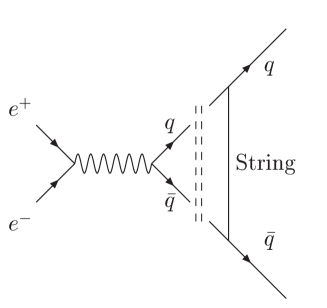
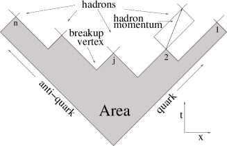
Figure 1: The figure shows a typical Lund String break-up.

• There is no field between a $q\bar{q}$-pair produced at a single vertex. A string force field is always confining because it has a fixed energy per unit length and the force field vanishes at the end-point charges.

• The hadrons must have positive momenta which implies, cf. Fig.1, that the vertices must be space-like separated. This means that no invariant time-ordering is possible. There is no principle ”first” vertex, they are all ”equal”. In the Lund Model, it will always be the slowest particles that are produced first in any frame.

Figure 2: Two adjacent vertices and a hadron with energy-momentum $p_{j}$ produced in between.

A convenient ordering prescription is rank-ordering. Two hadrons that share the same vertex will be defined to have adjacent rank. If one starts to count from the original quark end, this means that the hadron which contains this quark and an anti-quark from a break-up vertex will have rank 1, cf. Fig.1. The break-up process can be described as a set of steps along the positive light-cone momentum, where each hadron takes a fraction $z_{j}$ of the remaining light-cone momentum, cf. Fig.2.

It is possible to calculate the probability for a string break-up inside the Lund String Model using the basic properties that we just have mentioned if one also includes a ”saturation assumption”, [1, 2, 3]. This additional assumption basically means that even if the energy of the original pair will increase without limit the distribution of the proper times of the production vertices will stay finite. The two main results are:

• The probability for producing a hadron with mass $m$ taking a fraction $z$ of the remaining (positive) light-cone momentum is given by $f(z)dz$, where

  $$f(z) = N\frac{1}{z}(1-z)^{a}exp(\frac{-bm^{2}}{z})$$ (1)

  $f$ is called the Lund Symmetric Fragmentation Function (probability distribution). We note that small $z$ values will be exponentially suppressed (with $\frac{1}{z}$), while large $z$ values will be power suppressed. The final result is that the vertices typically will be along a hyperbola in space-time in the Lund Model.

• The Area Law, which states that the (non-normalised) probability to produce a set of hadrons with momenta $p_{1},p_{2},\ldots,p_{n}$ and total momentum $P_{tot}$ is given by:

  $$dP_{n}(\{p_{j}\};P_{tot})=\prod_{j=1}^{n}N_{j}d^{2}p_{j}\delta({p_{j}}^{2}-{m_{j}}^{2})\delta(\sum_{j=1}^{n}p_{j}-P_{tot})\exp(-bA)$$ (2)

  , i.e. the phase-space times a negative exponential of an area. The area is the area spanned by the string state before it decays, cf. Fig.1.

Figure 3: The vertex V will subdivide the system into ”right-movers” ($p_{1},\ldots,p_{j}$) and ”left-movers” ($p_{j+1},\ldots,p_{n}$).

           

  Figure 4: The production process described in terms of momentum transfers.

Up to this point, we have described the break-up process in space-time. We are now going to show that one can also describe the same process in momentum space. In order to do this, we first note that a vertex (V) subdivides the state into $\underbrace{\{p_{n},\ldots,p_{j+1}\}}_{\mathrm{{}^{\prime\prime}to\,the\,left^{\prime\prime}}}\oplus\underbrace{\{p_{j},\ldots,p_{1}\}}_{\mathrm{{}^{\prime\prime}to\,the\,right^{\prime\prime}}}$, cf. Fig.3. From this figure we conclude that:

$$p_{1}+p_{2}+\ldots+p_{j}=(W^{+}-X^{+},X^{-})$$ (3)

$$p_{j+1}+\ldots+p_{n}=(X^{+},W^{-}-X^{-})$$

We can therefore describe the process according to the left-hand figure in Fig.4, if we define the momentum transfer $q\equiv(X^{+},-X^{-})$. This process can be repeated for any vertex. This means that String Fragmentation can be described as a ladder diagram like the one in the right-hand figure of Fig.4. There is a duality relationship between the space-time picture and this last diagram, cf. the left-hand figure of Fig.5.

Figure 5: One possible way to partition the area of a fragmenting string into contributions for each hadron. It shows the connection between the area in the area law and the area between the directrix and the hadronic curve.

2 Fragmentation of Gluonic Strings

Presence of internal gluonic excitations cause the string to trace complex curved surfaces in space–time. Approximating the partonic state with a finite number of gluons with transverse momenta above a certain scale is equivalent to approximating the curved surface of a string by a set of planar regions with the (scaled) parton energy momenta at the boundaries. The dynamics of such a string is most conveniently described in terms of the action principle which implies that the string world surface should be a minimal area surface.

This means that the details of the string world surface are completely determined by a specification of the boundary, i.e., the quark or anti-quark world lines. For an open string these two world lines differ by just a translation, and hence it is sufficient to specify only one of them. This boundary curve is called the directrix. The position of an arbitrary point $X(t,\sigma)$ on the surface of the string (parametrised by time ’$t$’ and the energy $\sigma$ between the point and the quark end point) is related to the directrix ${\cal A}(t)$ in the following way.

$$X(t,\sigma) = \frac{1}{2}\left({\cal A}(t+\sigma)+{\cal A}(t-\sigma)\right)$$ (4)

The function ${\cal A}(t)$ has the following periodicity and symmetry properties for a string which starts at a single point:

$${\cal A}(t+2E) = {\cal A}(t)+2P$$ (5)

$${\cal A}(-t) = -{\cal A}(t)$$

We see from Eq.(4) and Eq.(5) that the string surface is described by a left moving and a right moving wave, which bounce at the endpoints. It can also be seen that the internal excitations would move and affect the end points in colour order. The directrix of a string stretched between a certain set of partons is therefore obtained by laying out the energy-momenta of the quark, the gluons and the anti-quark in colour order.

The minimal area nature of the string world surface also means that properties of hadrons created during string fragmentation are stable against small perturbations on the boundary, i.e. that the model is infrared stable.

Since the directrix describes the string state, hadronisation of a string can be formulated as a process along the directrix. In [4] we presented one such formulation of string fragmentation, and we briefly mention some of the main ideas here.

In [4], we defined an iterative process along the directrix to describe string fragmentation. We defined (abstract) dynamical variables called “vertex” vectors $x_{i}$. These variables would correspond to true space-time locations for production of quark anti-quark pairs if the string had no gluonic excitations. Each particle energy-momentum vector $p_{i}$ is constructed as a linear combination of a vertex vector $x_{i-1}$ and a certain section of the directrix $k_{i}$. The same pair of vectors $x_{i-1}$ and $k_{i}$ also determines the next vertex vector $x_{i}$.

$$p_{i}=z_{i}x_{i-1}+\frac{1}{2}(1-\frac{z_{i}^{2}x_{i-1}^{2}}{m_{i}^{2}})k_{i}$$ (6)

$$x_{i}=(1-z_{i})x_{i-1}+\frac{1}{2}(1+\frac{z_{i}^{2}x_{i-1}^{2}}{m_{i}^{2}})k_{i}$$

Since with this construction, $x_{i-1}+k_{i}=p_{i}+x_{i}$, we associate a “plaquette” bounded by those four vectors with the particle indexed “i”. Each of the vectors $x_{i}$ is shared between two plaquettes, and hence production of a set of hadrons from a given string or directrix means construction of a set of connected plaquettes along the directrix in this model. The initial value $x_{0}$, for the series of vertex vectors, is taken to be the first segment of the directrix. The numbers $z_{i}$ are related to the area of the plaquettes.

There is a one to one correspondence between the areas of the plaquettes constructed in this way and certain areas which can be associated with the production of individual hadrons in the string fragmentation model without gluonic excitations. Therefore, the sum of the areas of the plaquettes, which is also the area between the directrix and the “hadronic curve” (i.e. the curve obtained by placing the hadron energy-momenta one after the other in rank order. We called this curve the $X$-curve in [4]), could be used as the area in the Lund Model area law. Therefore, area law on the whole event can be implemented by weighting the construction of each plaquette according to its area, which amounts to choosing the variables “$z_{i}$” in Eq.(6) according to the Lund symmetric fragmentation function.

It was shown in [4] that in the limit of infinitesimal steps $k_{i}$ along the directrix, the hadronic curve approaches a continuous curve in space–time which we called a $P$-curve. This could be thought of as the equivalent of the average hyperbolical fragmentation region in a simple gluon-less string fragmentation scheme in this model. There is a close connection between the $P$-curve and a certain ${\cal X}$-curve defined on the partonic state, or the directrix. The ${\cal X}$-curve and its length, called the $\lambda$-measure which is related to the available phase space for hadron production, are easily calculated for a given directrix. It is apparent therefore that the average hadronic curve in this model is determined by perturbative calculations.

3 Generalised Dipoles

In this section we will discuss certain properties of the QCD bremsstrahlung mostly in connection with the dipole cascade model as implemented in the Monte Carlo routine Ariadne and relate them to the hadronisation procedure we have just mentioned.

Gluon radiation from QCD colour dipoles can be compared to photon radiation from electromagnetic dipoles. The inclusive density for the emission of a gluon from a quark anti-quark dipole is given by

$$dn=\alpha_{\mathrm{eff}}\cdot\frac{dk_{\perp}^{2}}{k_{\perp}^{2}}\cdot dy\cdot(\mathrm{PolarisationSum})$$ (7)

This is very similar to the result for photons. Energy momentum conservation implies that the transverse momentum and rapidity of the emitted particle obey the following constraint:

$$k_{\perp}cosh(y)\leq\frac{\sqrt{s}}{2}$$ (8)

where $\sqrt{s}$ is the center of mass energy of the dipole. This in turn, means that the total rapidity range available for the emission is given by

$$\Delta y\approx ln\left(\frac{s}{k_{\perp}^{2}}\right)$$ (9)

The emission of a photon leaves the electromagnetic current unchanged except for small recoil effects, whereas the emission of a gluon, which has colour charge, changes the current for further gluon radiation. However, it was shown in [7, 8] that to a very good approximation, the density for the emission of two gluons can be written as the product of two contributions.

$$dn(q,g_{1},g_{2},\bar{q})=dn(q,g_{1},\bar{q})\left[dn(q,g_{2},g_{1})+dn(g_{1},g_{2},\bar{q})-\mathrm{small\ correction}\right]$$ (10)

Emission of two gluons could therefore be described as the emission of one first gluon from the original quark anti-quark pair, and the subsequent emission of the second gluon of smaller transverse momentum, from one or the other colour dipole involving the doubly (colour) charged gluon. In other words, the emission of the first gluon splits the original colour dipole into two dipoles which radiate independently.

The available rapidity range for the emission of the second gluon, which is just the sum of the rapidity ranges available in the two dipoles available after the first emission, is more than the rapidity range in the original quark anti-quark dipole.

$$\Delta y(g_{2})=ln\left(\frac{s_{qg_{1}}}{k_{\perp}^{2}}\right)+ln\left(\frac{s_{g_{1}\bar{q}}}{k_{\perp}^{2}}\right)=ln\left(\frac{s}{k_{\perp}^{2}}\right)+ln\left(\frac{\frac{s_{qg_{1}}s_{g_{1}\bar{q}}}{s}}{k_{\perp}^{2}}\right)$$ (11)

The quantity $s_{qg_{1}}s_{g_{1}\bar{q}}/s$ is the invariantly defined transverse momentum of the first gluon. Eq.(11) therefore implies that the emission of the first gluon increases the available phase space for further gluon emission by an amount $ln(k_{\perp 1}^{2}/k_{\perp}^{2})$.

Figure 6: The triangular Lund phase-space diagrams described in the text.

The above dipole splitting scenario is generalised in the dipole cascade model. Emission of the second gluon is thought to give rise to three dipoles which radiate independently, and so on. The available rapidity range for emission of new gluons at a certain transverse momentum scale $k_{\perp}$ is, as a consequence of Eq.(11), a function of all the emissions above that scale.

$$\Delta y(g_{n})=ln(\frac{s}{k_{\perp^{2}}})+\sum_{i=1}^{n-1}ln(\frac{k_{\perp i}^{2}}{k_{\perp}^{2}})$$ (12)

The increase of phase space due to gluon emission is conveniently visualized using the Lund triangular phase space diagrams, such as those shown in Fig.6. The $y$-axis represents the logarithm of the transverse momentum scale $k_{\perp}^{2}$, denoted by $\kappa$. Eq.(9) then means that as $\kappa$ is decreased the available phase space increases linearly with $-\kappa$. This is represented by the base line of the triangle which increases as $kappa$ decreases. In the second figure, we show one gluon emitted at a certain scale $\kappa_{1}$. The phase space for emission at a lower scale is the base line of the original triangle plus another term which increases linearly with $\kappa_{1}-\kappa$ according to Eq.(11). This is represented by the additional triangular appendage starting at $\kappa_{1}$. The total phase space is therefore obtained by measuring the length of the base line of the structure, going around all triangular appendages. The third figure in Fig.6 shows this after several emissions. The forth figure is a view from the “bottom” of the phase space triangle. The triangular appendages appear as lines coming out of the original base line, increasing its length.

The transverse momentum scale $\kappa$ is a resolution scale on the partonic state. The smaller the scale, the softer the gluons we resolve. Fig.6 illustrates that the available phase space scales such that it increases faster than a linear rate when the resolution scale is lowered. This is a manifestation of the anomalous dimensions of QCD.

It should be noted that the phase space in Eq.(12) is not written in terms of variables describing the state from which further emission is being considered. It requires information about the history of the event, i.e. which gluon was emitted first, which came next etc., and at what transverse momenta they were emitted. It also ignores the effect of recoil due to gluon emissions. For a small invariant mass of the radiating dipole, recoil effects could be significant. Emission from any one dipole would give a recoil to the two partons in that dipole, and would therefore change the mass of the adjoining dipoles. The assumption of independent emission from the dipoles itself, however provides one measure defined in terms of the dipoles available for radiation:

$$\ell(k_{\perp}^{2})=\sum^{\mathrm{dipoles}}\ln\frac{s_{\mathrm{dipole}}}{k_{\perp}^{2}}$$ (13)

When a string without gluons decays, the rapidity range available to hadrons along the mean hyperbolic decay region is given by an expression similar to Eq.(9), with the transverse momentum scale $k_{\perp}^{2}$, replaced by a suitable scale $m_{0}^{2}$ related to hadronisation. But generalisation of the phase space available for hadron formation goes along slightly different lines. One observes that the hadronisation scale $m_{0}^{2}$ is independent of the scale at which the partonic state is calculated. Since string fragmentation is infrared stable, the phase space for hadrons should be an infrared stable generalisation of the flat string phase space, as softer and softer gluons are added. Addition of gluons softer than the scale $m_{0}^{2}$ should not affect the phase space significantly.

Such a generalisation was developed in [5], and has been discussed over the years. This measure, called the $\lambda$-measure, is defined in terms of differential equations for a general directrix ${\cal A}(\xi)$ as follows. We define a four-vector valued functional $q_{T}$ and a scalar valued functional $T$ :

$$T(\xi)=1+\int_{0}^{\xi}\frac{d{\cal A}(\xi_{1})\cdot d{\cal A}(\xi_{2})}{m_{0}^{2}}\theta(\xi_{1}-\xi_{2})T(\xi_{2})$$ (14)

$$q_{T}(\xi)=\frac{1}{T(\xi)}\int_{0}^{\xi}d{\cal A}(\xi^{\prime})T(\xi^{\prime})$$ (15)

which satisfy the differential equations:

$$dT = \frac{q_{T}d{\cal A}}{m_{0}^{2}}T$$

$$dq_{T} = d{\cal A}-\frac{q_{T}d{\cal A}}{m_{0}^{2}}q_{T}$$

$$dq_{T}^{2} = 2(1-\frac{q_{T}^{2}}{m_{0}^{2}})q_{T}d{\cal A}$$ (16)

They can be integrated to:

$$T(\xi) = \exp\left(\int_{0}^{\xi}\frac{q_{T}(\xi^{\prime})d{\cal A}(\xi^{\prime})}{m_{0}^{2}}\right)$$

$$q_{T}^{2}(\xi) = m_{0}^{2}[1-T(\xi)^{-2}]$$ (17)

Finally we note that we may define a four-vector valued function ${\cal X}_{\mu}={\cal A}_{\mu}-q_{\mu}$ so that:

$$d{\cal X}=\frac{(q_{T}d{\cal A})}{m_{0}^{2}}q_{T}$$ (18)

Thus the vector $q_{T}$ is the tangent to the ${\cal X}$-curve reaching out to the directrix. From Eq.(3) we conclude that the functional $T$ is the exponential of an area (note that the vector $d{\cal A}$ is light-like, and $qd{\cal A}$ is an area element between the directrix and the ${\cal X}$-curve). This area corresponds to the measure $\lambda$ mentioned earlier. We also note that the vector $q_{T}$ quickly reaches the length $m_{0}$. Integrating the differential equations for a directrix built up from a set of light-like vectors $\{k_{j}\}$ we obtain the iterative equations:

$$T_{j+1} = T_{j}(1+q_{Tj}k_{j+1}/m_{0}^{2})\equiv\frac{T_{j}}{\gamma_{j+1}}$$

$$q_{Tj+1} = \gamma_{j+1}q_{Tj}+\frac{1+\gamma_{j+1}}{2}k_{j+1}$$ (19)

The starting values are $T_{0}=1$ and $q_{T0}=k_{0}$.

The factorisability of the functional $T$ means that its logarithm, $\lambda$, can be written as a sum containing one term for each $k_{j}$:

$$\lambda\equiv\sum_{j=1}^{n+1}\Delta\lambda_{j}=\sum_{j=1}^{n+1}\ln\left(1+q_{Tj-1}k_{j}/m_{0}^{2}\right)$$ (20)

Figure 7: A plaquette bordered by $q_{Tj}$, $q_{Tj+1}$ , $k_{j}$ and a hyperbolic segment from the ${\cal X}$-curve, as described in the text.

The $\Delta\lambda_{j}$ defined in this way corresponds to the size of a subarea just as the total $\lambda$ corresponds to the area spanned between the ${\cal X}$ and the directrix curves. In Fig. 7 we exhibit such a region or “plaquette” bordered by the “initial” $q_{Tj}$ and the “final” $q_{Tj+1}$ together with a hyperbolic segment from the ${\cal X}$-curve and the gluon energy-momentum vector $k_{j}$ from the directrix.

Eq.(20) should be compared with Eq.(13). Eq.( 13) expresses the gluon emission phase space as a sum of contributions, one term for each colour dipole. Eq.(20) expresses the infrared stable hadronisation phase space as a sum of contributions, one term for each vector along the directrix, or one term for each plaquette as mentioned in the previous paragraph. With this analogy in mind we called these plaquettes “Generalised Dipoles”(GD) in [6]. The hadronisation procedure outlined in Sec. 2 could be thought of as a procedure which divides these GDs into smaller plaquettes, one for each hadron. In [6] we discussed further the similarities and differences between the $\lambda$-measure, and the $\ell$-measure.

In [6] we have also reported on some interesting scaling properties of the contributions to the $\ell$-measure from individual dipoles. It was found that for partonic states obtained from parton showers in Monte Carlos like Pythia and Ariadne, the dipole sizes measured relative to the transverse momentum cut-off scale $k_{\perp}$ had a distribution which was surprisingly insensitive to the scale $k_{\perp}$ cf. Fig.8. We showed that it is possible to understand the distributions in terms of a “gain-loss” analysis: as we go down in transverse momentum, the dipole sizes increase, since they are measured relative to transverse momentum. But emission of softer gluons would split some dipoles of a given size into smaller ones which are lost from a certain bin in dipole size. The same process would split some dipoles of larger size, so that they end up in the bin under consideration. An integro differential equation taking into account these considerations reproduces the observed behaviour in dipole sizes quite well, as illustrated in Fig.8.

Figure 8: Dipole sizes obtained from Pythia  and Ariadne , measured relative to the cut-off scales, are relatively insensitive to the cut-off scales. The behaviour is quite well described by an MLLA calculation.

It was also found that the contributions to the $\lambda$-measure from individual GDs have very similar scaling properties, if the scale $m_{0}^{2}$ is chosen to be proportional to the ordering variable in the parton cascade. Even though there is no direct way to calculate the distribution of sizes for GDs, in the light of certain similarities between the $\lambda$-measure and the $\ell$-measure, such behaviour is not completely unexpected.

That parton showers tend to produce structures of the same size relative to the cut-off scale is interesting because the $\lambda$-measure and the Generalised Dipoles are connections between perturbative physics and hadronisation. On the one hand they are related, and share many properties with phase space for gluon emission. On the other hand the fragmentation process reviewed in Sec.2 is a connection between the plaquettes we called GDs and the plaquettes we defined for each hadron in Sec.2. Properties of the colour dipoles which are preserved in the Generalised Dipoles will be carried over to the final state hadrons.

4 Conclusions

String fragmentation can be formulated as the production of a set of “plaquettes” between the partonic curve or directrix, and the hadronic curve. The sum of the areas of the plaquettes is taken as the area in the Lund Model area law. The mean size of this total area can be calculated from the specified perturbative state, and is proportional to the length of a curve called the ${\cal X}$-curve. The length of the ${\cal X}$-curve is also called the $\lambda$-measure. The ${\cal X}$-curve looks like a set of connected hyperbolae stretching across planar regions around the directrix which we called “Generalised Dipoles”. The size of the GDs measured relative to the parton shower cut-off scale seems to have a distribution which is insensitive to the cut-off scale itself. This can be understood as a balance between emission of more gluons at a softer scale versus the scaling of the phase space variable itself.

References

- [1] B. Andersson, G. Gustafson and C. Peterson, Z. Phys. C1 (1979) 105.
- [2] B. Andersson, G. Gustafson and B. Söderberg, Z. Phys. C20 (1983) 317.
- [3] B. Andersson, The Lund Model, Cambridge University Press, 1998.
- [4] B. Andersson, S. Mohanty and F. Söderberg, Eur. Phys. J. C21 (2001) 631.
- [5] B. Andersson, G. Gustafson and B. Söderberg, Nucl. Phys. B264, 29 (1986).
- [6] B. Andersson, S. Mohanty and F. Söderberg, Accepted for publication in Nucl. Phys. B. (hep-ph/0207025).
- [7] Ya.I. Azimov et al. Phys. Lett. B165 (1985) 147
- [8] Yu.L. Dokshitzer, V.A. Khoze, A.H. Mueller and S.I. Troyan, Basics of Perturbative QCD (Edition Frontières 1991).