Abstract

We study the resummation of large QCD radiative corrections up to the next to leading logarithmic accuracy to the process $\gamma\gamma\to b\bar{b}$; i.e., we resum logarithms of the type $\alpha_{s}^{p}\ln^{2p}{m^{2}/s}$ and $\alpha_{s}^{p}\ln^{2p-1}{m^{2}/s}$ ($m$ is the quark mass). The only source of all the logarithms to this accuracy is the off-shell Sudakov form factor included into the triangle topologies of the one-loop box diagram. We prove that any other configurations of diagrams to this accuracy, either cancel in subgroups or develop a universal on-shell Sudakov exponent due to the final quark anti-quark lines. We study the mechanism of cancellations between the different diagrams, which leads to the simple resummed results. We show the cancellation explicitly at three loops for the leading and at two loops for the next-to-leading logarithms. We also point out the general mechanism responsible for it, and discuss how it can be extended to higher orders.

^ae-mail: akhoury@umich.edu
^be-mail: haibinw@umich.edu
^ce-mail: yakovlev@umich.edu

1 Introduction

Future Linear Colliders are expected to reveal the answers to many questions of modern particle physics. One of these concerns the the physics of the Higgs particle and origin of electroweak symmetry breaking. The neutral scalar Higgs boson is an important ingredient of the Standard Model (SM) and is the only SM elementary particle which has not been detected so far (see for a review [1], [2]). The lower limit on $m_{H}$ of approximately $113.5$ GeV at $95\%$ c.l. has been obtained from direct searches at LEP [3]. Current experiments are concentrating on the possibility of finding a Higgs particle in the intermediate mass region $113.5<m_{H}<150\quad\mbox{GeV}.$ In this region it decays mainly to a $b\bar{b}$ pair.

The photon mode of the future Linear Collider (LC), namely the collisions of the energetic polarized Compton photons, will be used for the production and for the study of the Higgs particle. In the intermediate mass range, the main production process is

$$\gamma\gamma\to H\to b\bar{b}.$$

QCD as well as electroweak radiative corrections to this process have been studied very well and have been found to be small in this region [4]. The main challenge, however, is to get under control the background process

$$\gamma\gamma\to b\bar{b},$$

which gets extremely large QCD corrections.

In this paper we discuss the process of the quark anti-quark production in the photon mode of the LC, $\gamma\gamma\to b\bar{b}$. The amplitude for this process in the scalar channel contains large double logarithms at $|s|,|t|,|u|\gg m^{2}$. At very high energies, the large logarithms spoil the perturbative predictions. Therefore it is mandatory to develop a clear resummation procedure for this double and single logarithmic terms. Let us stress, that the main interest in the process $\gamma\gamma\to b\bar{b}$ comes from the fact (but is not limited to it) that it represents the dominant background for the production of the Higgs particle, $\gamma\gamma\to H\to b\bar{b}$ [5, 6, 7]. In fact, our motivations for this study are twofold:
(1) A detailed study of the process $\gamma\gamma\to b\bar{b}$ is very important due to phenomenological reasons mentioned above; and
(2) in addition to that, the quark anti-quark production in photon collisions , being one of the simplest process in QCD, is important in its own right, e.g. for studying and understanding QCD effects.

The Born cross section for the polarized $b\bar{b}$ production in the scalar channel (at $J_{z}=0$), where the Higgs will be studied as well, is suppressed by $\frac{m_{b}^{2}}{s}$ [8, 9], (here $s$ is the center of mass energy of the initial photons). However, the perturbative QCD corrections contains the large double logarithms of the form $\rho=\alpha_{s}\ln^{2}(\frac{m_{b}^{2}}{s})$, which give a contribution to the cross section which is of the same order as the Born contribution at high energies. The presence of the large correction was noticed by Jikia in [9]. The double logarithmic nature and the origin of these corrections were studied in [7]. The authors studied the process to one and two loop accuracy. Later, the form of the resummed results for the double logarithms has been argued in [10]. These authors also claimed that the double logarithms have a“non-Sudakov” origin.

In this paper, we first present an alternative way of understanding the resummation procedure for the double logarithms. The general idea of our approach, is that the only source of double logarithms is the off-shell Sudakov form factor included in the triangle topologies of the one-loop box diagram. We have proved that the other types of the higher loop diagrams will either cancel in subgroups or develop a universal on-shell Sudakov exponent due to the final quark anti-quark lines. In addition to that, (1) we extend this analysis to the next-to-leading-logarithmic (NLL) accuracy, and (2) we study the mechanism of cancellations alluded to above, between the different diagrams which leads to very simple resummed results. We demonstrate the cancellation explicitly at three loops and point out the mechanism responsible which then allows for the generalization to higher loops, all up to the next to leading logarithmic accuracy. As an aside, we argue that all the large logarithms up to the next to leading level are related to the Sudakov ones. This includes not only the leading ones of the form $\alpha_{s}^{p}\ln^{2p}{m^{2}/s}$ but also the next to leading ones of the form $\alpha_{s}^{p}\ln^{2p-1}{m^{2}/s}$ ($m$ is the quark mass). It is this fact together with an understanding of the cancellation mechanism which allows us to develop an easy resummation procedure.

The paper is organized as follows. In section 2.1 we discuss the one loop diagrams and explain which topologies are important. In section 2.2 we present a procedure for the resummation of the double logarithms. In section 2.3 we extend our analysis to the next-to-leading logarithmic level. In this section we consider all possible topologies and give the final result of the resummation. Section 3 is devoted to the study of the different cancellations which are responsible for the simple resummed results of section 2.2 for the double logarithmic case. In section 4 we tackle the case of the form factors to the next to leading logarithmic accuracy and justify the results given in section 2.3. The paper ends with some conclusions and discussions.

2 The resummation up to next to leading logarithms

2.1 One loop results

We study the process of quark anti-quark pair production in photon-photon collisions

$$\gamma(k_{1})+\gamma(k_{2})\to q(p_{1})+\bar{q}(p_{2})$$ (1)

in the scalar channel $J_{z}=0$, at very high energies compared to the mass of the quark $m$, and at large scattering angles

$$|s|\sim|t|\sim|u|\gg m^{2}.$$ (2)

The radiative corrections to this helicity amplitude contain large double and single QCD logarithms of the form $\alpha_{s}\ln^{p}(s/m^{2}),p=2,1$, in the limit eq.(17,18).

It has been shown in [7] that the large double logarithms (DL) have a Sudakov-like nature and can be extracted from the total result by identifying special kinematic regions. It was demonstrated that, only the box diagram contributes, and that this box diagram can be reduced to three different effective diagrams with triangle topology. We label them as topologies A,B,C following [7], see Fig.(1). These effective diagrams result from the box diagram when one of the four propagators is hard, two collinear and one soft ( the soft line can be either the gluon or the quark propagator). Hence one can shrink the hard propagator of the box diagram to a point, because it does not depend on the soft loop momenta anymore. The hard momenta would be just an ultra violet cutoff in this situation.

In order to introduce notations and to get an idea about the structure of the DL, let us consider one loop calculations in the DL approximation. Also, we will use these results in the next section for the construction of the DL-resummed result.

Figure 1: Triangle topologies obtained from the one loop box diagram.

As is well known, the double logarithms come from the region of soft loop momenta. Hence, one can always write a factorized form for the amplitude in the DL approximation:

$$M_{A}=M_{\mbox{Born}}\cdot F_{A},\qquad M_{B}=M_{\mbox{Born}}\cdot F_{B},\qquad M_{C}=2M_{\mbox{Born}}\cdot F_{C},$$ (3)

the factor 2 in the last equation represents two identical contributions $C_{1},C_{2}$ of the topology C. The amplitude then reads

$$M=M_{\mbox{Born}}\cdot\Big{(}F_{A}+F_{B}+2F_{C}\Big{)}.$$ (4)

We turn now to the calculation of the form factors $F_{A},F_{B},F_{C}$.

It is convenient to use the standard Sudakov technique for calculating DL contributions, as described in [11, 7], and introduce Sudakov parameterization [11, 12]. One starts with decomposing the soft momenta in terms of those along the hard external momenta, for example $k_{1},k_{2}$ and transverse to them

$$k=\alpha k_{1}+\beta k_{2}+k_{\bot}.$$ (5)

The DL contribution comes only from the region

$$m^{2},|k_{\bot}|^{2}\ll s|\alpha|,s|\beta|\ll s.$$ (6)

For different topologies it is convenient to use different decompositions of the soft momenta:

$$\mbox{topology A:}\qquad k = \beta(p-\frac{m^{2}}{s}\bar{p})+\alpha(\bar{p}-\frac{m^{2}}{s}p)+k_{\bot}$$ (7)

$$\mbox{topology B:}\qquad k = \beta k_{2}+\alpha k_{1}+k_{\bot}$$ (8)

$$\mbox{topology C:}\qquad k = \beta k_{2}+\alpha(\bar{p}-\frac{m^{2}}{s}k_{2})+k_{\bot}$$ (9)

The loop integration in terms of the new variables reads

$$\int\limits_{-\infty}^{\infty}d^{4}k=\frac{s}{2}\int\limits_{-\infty}^{\infty}d\alpha\int\limits_{-\infty}^{\infty}d\beta\int\limits_{0}^{\infty}\pi dl^{2}_{\bot}.$$ (10)

The integration over the transverse momenta of the soft quark is performed by taking half of the residues in the corresponding propagator,

$$\int\frac{d^{4}k}{k^{2}-\lambda^{2}+i0}F=\int\frac{s}{2}\frac{d\alpha d\beta d^{2}k_{\bot}}{s\alpha\beta-k_{\bot}^{2}-\lambda^{2}+i0}F\to-i\pi^{2}\frac{s}{2}\int d\alpha d\beta\Theta(s\alpha\beta-\lambda^{2})F,$$ (11)

here $\lambda$ is a small (fictitious) gluon mass. In this manner the one loop amplitude may be calculated in the DL approximation and topology A gives,

$$F^{1-loop}_{A} = -\frac{C_{F}\alpha_{s}}{2\pi}\int\limits_{0}^{1}\int\limits_{0}^{1}\frac{d\alpha d\beta}{\alpha\beta}\Theta(\alpha\beta-\frac{\lambda^{2}}{s})\Theta(\alpha-\frac{\lambda^{2}}{s}\beta)\Theta(\beta-\frac{\lambda^{2}}{s}\alpha)$$ (12)

$$= -\frac{C_{F}\alpha_{s}}{2\pi}\Big{(}\frac{1}{2}\ln^{2}\frac{m^{2}}{s}+\ln\frac{m^{2}}{s}\ln\frac{\lambda^{2}}{m^{2}}\Big{)},$$ (13)

Topology B and C have following form at one loop in the DL approximation

$$F^{1-loop}_{B}=F^{1-loop}_{C} = -\frac{C_{F}\alpha_{s}}{2\pi}\int\limits_{0}^{1}\int\limits_{0}^{1}\frac{d\alpha d\beta}{\alpha\beta}\Theta(\alpha\beta-\frac{m^{2}}{s})=-\frac{C_{F}\alpha_{s}}{2\pi}\Big{(}\frac{1}{2}\ln^{2}\frac{m^{2}}{s}\Big{)}$$ (14)

These results were derived first in [7] and will be used in our calculation later on.

2.2 The double logarithmic resummation

The main idea behind our method is that the only origin of the double logarithms is the off-shell Sudakov form factor included in the effective one loop triangle diagrams A,B and C. Contributions from other types of diagrams will either cancel in subgroups or develop a simple on-shell Sudakov exponent due to the final quark anti-quark pair. The cancellations amongst the diagrams will be discussed in the next section where the general mechanism is elucidated. Here we study the DL resummation in the topologies A, B and C.

The diagrams of topology A represent a simple case. Here we do not have any “hard” DLs, but only the “soft” ones, which develop the usual on-shell Sudakov form factor from the gluon exchanges between the final quark antiquark pair. It is well known, that the on-shell DL Sudakov form factor in QCD is the exponent of the one loop result

$$F_{A}=\mbox{Exp}\Big{(}F^{1-loop}_{A}\Big{)},$$ (15)

with $F^{1-loop}_{A}$ given in eq.(12).

The resummation of the DL terms coming from the diagrams of topology B is more involved. First, we have to account for the “soft” on-shell exponent from the final quark antiquark re-scattering, similar to the one in topology A, eq.(15). Second, we observe a new element, namely the “hard” double logarithms from quark anti-quark re-scattering inside the one loop diagram. The interacting particles (quarks in this case) are hard and slightly off-shell, $p_{1,2}^{2}\ll s$.

According to our general idea, the resummation of the “hard” DL can be obtained by including the off-shell Sudakov form factor into the loop, and accounting only for those momenta which do not destroy the DL nature of the one loop result.

We recall that the off-shell Sudakov form factor, is a vertex of the production of the quark and anti-quark with small virtualities $p_{1}^{2}$ and $p_{2}^{2}$ and has a form [13]

$$S(p_{1},p_{2})=\mbox{Exp}\Big{(}-\frac{C_{F}\alpha_{s}}{2\pi}\ln(\frac{s}{|p_{1}|^{2}})\ln(\frac{s}{|p_{2}|^{2}})\Big{)},$$ (16)

assuming that $m^{2}\ll|p_{1}|^{2},|p_{2}|^{2}\ll s.$ Now the momenta $p_{1}$ and $p_{2}$ become loop momenta, i.e.,they depend on $\alpha,\beta$

$$p_{1}^{2}=(k_{1}+k)^{2}=s\beta,\qquad p_{2}^{2}=(k_{2}-k)=-s\alpha.$$ (17)

Because of the DL approximation, the kinematic region of interest is restricted by the inequalities

$$m^{2}\ll|p_{1}|^{2},|p_{2}|^{2}\ll s.$$ (18)

Taking into account the result eq.(16) and including it into eq.(14) we get

$$F_{B} = -\frac{C_{F}\alpha_{s}}{2\pi}\int\limits_{0}^{1}\int\limits_{0}^{1}\frac{d\alpha d\beta}{\alpha\beta}\Theta(\alpha\beta-\frac{m^{2}}{s})\mbox{Exp}\Big{(}-\frac{C_{F}\alpha_{s}}{2\pi}\ln|\alpha|\ln|\beta|\Big{)}$$ (19)

We next transform the exponent into a power series and find that the integral of the $n-$th term will be of the form

$$\int\limits_{0}^{1}d\xi_{1}\int\limits_{1-\xi_{1}}^{1}d\xi_{2}\xi_{1}^{n+a}\xi_{2}^{n+b}=\frac{\Gamma(n+a+1)\Gamma(n+b+1)}{\Gamma(3+2n+a+b)}.$$ (20)

The final result at DL accuracy reads

$$F_{B} = F_{B}^{\mbox{1-loop}}\sum\limits_{n=0}^{\infty}\frac{2\Gamma(n+1)}{\Gamma(2n+3)}\Big{(}-\rho_{B}\Big{)}^{n}$$ (21)

with $\rho_{B}=\frac{C_{F}\alpha_{s}}{2\pi}L^{2},L=\ln\Big{(}\frac{m^{2}}{s}\Big{)}$. The index $n$ shows that the order of the amplitude is $\alpha_{s}^{n}$. We can clearly identify the separate contributions of the fixed orders in $\alpha_{s}$. On the other hand, if $\rho_{B}$ is large all terms in the series are important, giving altogether some analytic function $F_{DL}(\rho)$. This function is identified with a hyper-geometric function ${}_{2}F_{2}(1,1;2,\frac{3}{2};z)$, namely

$$F_{B} = F^{1-loop}_{B}\sum\limits_{n=0}^{\infty}\frac{2\Gamma(n+1)}{\Gamma(2n+3)}\Big{(}-\rho_{B}\Big{)}^{n}={}_{2}F_{2}(1,1;2,\frac{3}{2},-\frac{\rho_{B}}{4})F^{1-loop}_{B}.$$ (22)

These functions are exact answers in $\rho_{B}$ in the DL approximation. For large values of the parameter $\rho$ the function $F_{DL}$ has the following asymptotic,

$$F_{B}(\rho_{B})=\frac{2\ln(2\rho_{B})}{\rho_{B}}F^{1-loop}_{B}.$$ (23)

Thus we see that despite the fact that perturbation theory blows up at large $\rho_{B}$, the resummed result gives a smooth well defined function.

Topology C differs from B only through the color structure at the DL level. At the end of the calculations the answers for topologies B and C are similar and are related by the simple substitution:

$$C_{F}\to C_{A}/2\quad\mbox{in the variable}\quad\rho_{B}.$$ (24)

Combining all results for the three topologies we have

$$M=M_{\mbox{Born}}(1+F_{B}+2F_{C})\mbox{Exp}\Big{(}F^{1-loop}_{A}\Big{)}.$$ (25)

with the functions defined above. We must stress that there are other diagrams which can give DL contributions. Fortunately, all of them cancel in the certain groups, as will be discussed in section 3. This cancellation has a very simple physical interpretation (see Sec. 3).

Our results are written in two different representations. We have checked that they are in agreement with [10], where the authors used a completely different method, not mentioning the off-shell Sudakov form factors at all. We believe that our approach is more transparent. It shows that the new double logarithms are of Sudakov type, and, therefore, the resummation procedure becomes simple. Another advantage of our approach is that it opens up the possibility for resumming the single logarithms as well.

2.3 Next-to-leading-logarithmic accuracy

It is possible to develop this approach to achieve next-to-leading-logarithmic accuracy.

First, the factorization formula should be modified in order to take into account single logarithms. The amplitude reads at NLL approximation

$$M=M_{\mbox{Born}}(1+\Delta+F_{B}+2F_{C})F_{A}$$ (26)

with the function

$$\Delta=\frac{\alpha_{s}C_{F}}{\pi}\frac{3}{2}\ln(s/m^{2}),$$

which can be extracted from the explicit calculations performed in [9] by expanding the result at $s=|t|=|u|\gg m^{2}$. $F_{A}$ is the on-shell Sudakov form factor to the next-to-leading logarithmic accuracy [14].

Second, in order to calculate the form factors $F_{B}$ and $F_{C}$ at NLL, we need an expression for the Sudakov form factor also to this accuracy. We turn now to the calculation of the form factors $F_{B}$ and $F_{C}$. In fact, such an analysis already exists in the literature [15] for the case when the two external fermion lines are off-shell by the same amount, i.e., $p_{1}^{2}=p_{2}^{2}=p^{2}$:

$$S_{NLL}(p,p)=\mbox{Exp}\Big{(}-\frac{C_{F}\alpha_{s}(p^{2})}{2\pi}\ln^{2}(\frac{s}{|p|^{2}})+\frac{3C_{F}\alpha_{s}(p^{2})}{4\pi}\ln(\frac{s}{|p|^{2}})\Big{)}.$$ (27)

For our purposes, we need to extend the analysis to take into account that $p_{1}^{2}\neq p_{2}^{2}$. It is easy to see that for the region, eq.(17), the proof of factorization and exponentiation given in [15] goes through with straightforward changes. The major change involves the normalization of the coupling. We have studied one and two loop diagrams for the $q\bar{q}$ production vertex with slightly off-shell quarks with the following result:

$$S_{NNL}(p_{1},p_{2}) = Exp\Big{(}-\frac{\alpha_{s}(\nu^{2})C_{F}}{2\pi}\Big{(}\ln\frac{|p_{1}|^{2}}{s}\ln\frac{|p_{2}|^{2}}{s}+\frac{3}{4}\ln\frac{|p_{1}|^{2}}{s}+\frac{3}{4}\ln\frac{|p_{2}|^{2}}{s}\Big{)}\Big{)},$$ (28)

with the normalization of the coupling constant determined to be $\nu^{2}=\sqrt{|p_{1}^{2}||p^{2}_{2}|}$. We show only the double and single IR logarithms in the exponent of eq.(28).

In order to understand this normalization, we have to consider the diagram shown in Fig.2

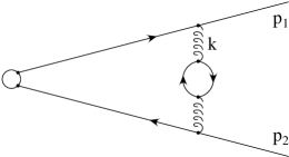
Figure 2: A diagram responsible for determining the normalization scale of the coupling constant.

where we keep track of the $n_{f}$ dependent pieces only since they are separately gauge invariant. Such diagrams can be accounted for by considering the following gluon propagator

$$D^{ab}_{\mu\nu}=-i\delta^{ab}(g_{\mu\nu}-\frac{k_{\mu}k_{\nu}}{k^{2}})\frac{1}{k^{2}}\frac{1}{1+\Pi(k^{2})},$$ (29)

where $\Pi(k^{2})$ is the vacuum polarization by the gluon; at the one loop level it is simply $\Pi=\frac{\alpha_{s}\beta_{0}}{4\pi}\ln\Big{(}\frac{k^{2}}{\mu^{2}}e^{C}\Big{)},\beta_{0}=11-\frac{2}{3}n_{f}$, $C$ being a scheme-dependent constant ($\overline{MS}$ scheme $C=-\frac{5}{3}$).

The diagram, Fig.2, corresponds to the first term in the expansion of the gluon propagator in $\alpha_{s}$. The $n_{f}$–part of this result is as mentioned earlier a gauge invariant subset of the complete set of two loop diagrams.

Because the effects of the running coupling gives only single logarithmic terms it is enough to consider the remaining integrals to DL accuracy. Namely, we may trace only the terms proportional to $\ln\frac{|p_{1}|^{2}}{s}\ln\frac{|p_{2}|^{2}}{s}$ from Fig.2. At the DL accuracy the spin structure of the amplitude is simple, so that one needs to consider the scalar integral only,

$$I=1+\frac{\alpha_{s}(\mu^{2})C_{F}}{2\pi}(2p_{1}p_{2})\int\frac{d^{4}k}{(2\pi)^{4}}\frac{1}{(p_{1}+k)^{2}}\frac{1}{(p_{2}-k)^{2}}\Big{(}1-\frac{\alpha_{s}\beta_{0}}{4\pi}\ln(\frac{k^{2}}{\mu^{2}})\Big{)}\frac{i}{k^{2}}.$$ (30)

To evaluate this, we consider a slightly more general integral

$$J=i\int\frac{d^{4}k}{(2\pi)^{4}}\frac{1}{(p_{1}+k)^{2}}\frac{1}{(p_{2}-k)}\frac{\mu^{2\Delta}}{(k^{2})^{1+\Delta}},$$ (31)

which after expanding in $\Delta$ will give us the desired integral $I$. Using Feynman parameters, this integral is reduced to

$$J=-\frac{1}{(4\pi)^{2}}\int\limits_{0}^{1}dy\frac{1}{A\Delta}\mu^{2\Delta}\Big{[}e^{-\Delta\ln(A+B)}-e^{-\Delta\ln(B)}\Big{]},$$ (32)

with

$$A(y)=p_{2}^{2}y^{2}+2p_{1}p_{2}y+p_{1}^{2},$$ (33)

$$B(y)=-2p_{1}p_{2}y-p_{2}^{2}y-p_{1}^{2},$$ (34)

$$A(y)+B(y)=p_{2}^{2}y(-1+y).$$ (35)

The function $A(y)$ has two zeros, $y_{\pm}$:

$$A=p_{2}^{2}(y-y_{+})(y-y_{-}),\quad y_{\pm}=\frac{-2p_{1}p_{2}\pm\sqrt{(2p_{1}p_{2})^{2}-4p_{1}^{2}p_{2}^{2}}}{2p_{2}^{2}}.$$ (36)

For very small virtualities, $p_{1}^{2},p_{2}^{2}\to 0$, the roots are simplified to $y_{+}=-\frac{p_{1}^{2}}{s},y_{-}=-\frac{s}{p_{2}^{2}}$. Expanding the integrand of $J$ in $\Delta$ up to second order we have

$$J = \frac{1}{(4\pi)^{2}}\int\limits_{0}^{1}dy\frac{1}{p_{2}^{2}(y-y_{+})(y-y_{-})}\mu^{2\Delta}\Big{(}\ln\Big{(}\frac{p_{2}^{2}y(1-y)}{(2p_{1}p_{2}+p_{1}^{2})y+p_{1}^{2}}\Big{)}$$ (37)

$$+ \frac{\Delta}{2}\Big{[}-\ln^{2}(p_{2}^{2}y(1-y))+\ln^{2}((2p_{1}p_{2}+p_{2}^{2})y+p_{1}^{2})\Big{]}\Big{)}.$$ (38)

The final integration over $y$ is simple, the result is

$$J = \frac{1}{(4\pi)^{2}2p_{1}p_{2}}\Big{(}-\ln\frac{|p_{1}|^{2}}{s}\ln\frac{|p_{2}|^{2}}{s}+\frac{\Delta}{2}\ln\frac{|p_{1}|^{2}}{s}\ln\frac{|p_{2}|^{2}}{s}\ln(\frac{|p_{1}^{2}||p_{2}^{2}|}{\mu^{4}})\Big{)}.$$ (39)

We see, that the first term in this equation reproduces the DL result from eq.(16) and eq.(28). It can be checked, that the second term suggests the normalization of the coupling constant to be, $\nu^{2}=\sqrt{|p_{1}^{2}||p_{2}^{2}|}$. Indeed, returning to the integral $I$, we find

$$I=1-\frac{\alpha_{s}(\mu^{2})C_{F}}{2\pi}\ln\frac{|p_{1}|^{2}}{s}\ln\frac{|p_{2}|^{2}}{s}\Big{[}1-\frac{\alpha_{s}(\mu^{2})\beta_{0}}{4\pi}\ln\Big{(}\frac{\sqrt{|p_{1}^{2}||p_{2}^{2}|}}{\mu^{2}}\Big{)}\Big{]}.$$ (40)

It is clear that the last logarithm, containing the $\beta_{0}$ term, can be absorbed into the running coupling, giving $\alpha_{s}(\nu^{2})$ with the normalization point $\nu^{2}=\sqrt{|p_{1}^{2}||p_{2}^{2}|}$. The exponentiation of the integral $I$ will give us the final off-shell Sudakov exponent, eq.(28).

In order to get single logarithms in eq.(28) we have to include the numerator and the spin structure. We do not present the details of these calculations here. Instead we note, that all logarithms we have accounted for are of infrared origin, $s\gg p_{1}^{2},p_{2}^{2}\to 0$. We do not show the UV logarithms which come as a result of the renormalization of the quark mass. Such terms can be omitted if the quark mass in the leading order result is normalized at a large scale $\mu^{2}=s$.

The formula eq.(28) reproduces the expression for the Sudakov form factor at non-equal virtualities at DL accuracy derived by Carrazone et. al. in [13], eq.(16), as well as at NLL with equal virtualities $p^{2}=p_{1}^{2}=p_{2}^{2}$ derived by Smilga in [15], eq.(27).

In addition, the normalization point $\nu^{2}=\sqrt{|p_{1}^{2}||p_{2}^{2}|}$ that we find reproduces that of the NLL results with equal virtualities $p^{2}=p_{1}^{2}=p_{2}^{2}$ derived by Smilga in [15], eq.(27).

This scale, $\nu^{2}=\sqrt{|p_{1}^{2}||p_{2}^{2}|}$, has a very transparent origin. The vertex of the interaction of a soft gluon with an off-shell quark ($p_{1}^{2}$) is described by the coupling $g(p_{1}^{2})$. In the situation of gluon-exchange between two quarks with different virtualities, we have an effective coupling $g(p_{1}^{2})g(p_{2}^{2})$. Using the running of the coupling $g^{2}(\mu^{2})=4\pi\alpha_{s}(\mu^{2})$, at one loop level, $\alpha(\mu^{2})=\alpha_{s}(\nu^{2})/(1+\frac{\alpha_{s}\beta_{0}}{4\pi}\ln(\frac{\mu^{2}}{\nu^{2}}))$, we will find that the effective coupling $g(p_{1}^{2})g(p_{2}^{2})$ is reduced to $\alpha_{s}(\sqrt{|p_{1}^{2}||p_{2}^{2}|})$, which coincides with our previous results.

As a next step, we include this form factor inside the one loop triangle diagram and calculate the last loop integration with the form factor which now accounts for all large logarithms to NLL accuracy. The final result for the next-to-leading-logarithmic form factor reads

$$F^{B}=F^{B}_{DL}+F^{B}_{NLL},$$ (41)

with $F^{B}_{DL}$ from eq.(21) and

$$F^{B}_{NLL} = \frac{1}{L}F^{1-loop}_{B}\sum_{n=0}^{\infty}\frac{\Gamma(n+1)}{\Gamma(2n+2)}(-\rho_{B})^{n}\Big{(}3-\frac{\rho_{B}\beta_{0}}{C_{F}}\frac{n}{2n+2}\Big{(}\frac{n+1}{2(2n+3)}+\frac{\ln(s/\mu^{2})}{L}\Big{)}\Big{)},$$ (42)

with $\beta_{0}=11-\frac{2n_{f}}{3}$, $n_{f}$ is the number of light flavors [16].

Topology C at NLL gives a slightly different result. In the previous section where we have already studied the DL result, we saw that the “hard” Sudakov form factor is developed as a result of the re-scattering of a hard quark on the hard gluon. Let us start with the Sudakov form factor for the quark-gluon vertex with an off-shell outgoing quark of virtuality $p_{1}^{2}$ and a gluon of virtuality $p_{2}^{2}$. The result for the reduced form factor is

$$S_{NNL} = Exp\Big{(}-\frac{\alpha_{s}(\nu^{2})C_{A}}{4\pi}\Big{(}\ln\frac{|p_{1}|^{2}}{s}\ln\frac{|p_{2}|^{2}}{s}+\ln\frac{|p_{1}|^{2}}{s}+\frac{1}{2}\ln\frac{|p_{2}|^{2}}{s}\Big{)}$$

$$+ \frac{\alpha_{s}C_{F}}{4\pi}(\ln\frac{|p_{1}|^{2}}{s}-\frac{a_{1}}{4C_{F}}\ln\frac{|p_{2}|^{2}}{s}\Big{)}\Big{)},$$

where the coefficient $a_{1}=\frac{10C_{A}}{3}-\frac{8T_{F}n_{F}}{3}$ is related to the wave function renormalization of the gluon. Now we can obtain a resummed result by substituting this form factor in the known one loop integral of topology C. The DL result coincides with that of topology B (as we discussed previously, after accounting for the substitution $C_{F}\to C_{A}/2$). The result for next-to-leading-logarithmic form factor reads

$$F^{C}_{NLL} = F^{1-loop}_{C}\sum_{n=0}^{\infty}\frac{\Gamma(n+1)}{\Gamma(2n+2)}(-\rho_{C})^{n}\Big{(}3-\frac{2C_{F}}{C_{A}}+\frac{a_{1}}{2C_{A}}$$

$$- \frac{2\rho_{C}\beta_{0}}{C_{A}}\frac{n}{2n+2}\Big{(}\frac{n+1}{2(2n+3)}+\frac{\ln(s/\mu^{2})}{L}\Big{)}\Big{)}$$

The final result for the amplitude is eq.(26) together with eq.(41,42,2.3). That concludes our derivation of the NLL form factors.

We emphasize that throughout this subsection we have taken into account all logarithms of the Sudakov type only. In section 4 we argue that to the NLL level this is justified because of cancellations between diagrams that is similar to the DL case. In other words, logarithms of the NLL type coming from other sources (than the Sudakov form factors) cancel between contributions of subsets of diagrams.

3 Cancellation mechanisms at the leading logarithmic level

The simple expressions for the resummed results given in the previous section are a consequence of the cancellation of double logarithmic terms which are not of the Sudakov type. In fact for the exponentiation to work there has to be a large number of cancellations between subgroups of diagrams. Such cancellations have been discussed in the literature explicitly at the two loop [7] and the three loop levels [10]. We agree with the results of these papers however the new element we would like to add here is to point out the general mechanism which is responsible for these cancellations. We discuss this mechanism on various examples and write down identities which guarantee the cancellations to higher loop orders.

3.1 The dipole mechanism for cancellation

The relevant cancellations at the double logarithmic level are due to a single mechanism - the dipole mechanism. Two fermions with opposite charges form a dipole when separated by a short distance. When observing from far away, or probing by means of a gluon with long wavelength, one finds the dipole system to be neutral to leading order. To be more specific, the total amplitude for exchanging a soft gluon with two such oppositely charged fermions, as shown by the sum of the two generic Feynman diagrams in Fig. (3), vanishes in the infrared sensitive region (double and single logarithms). This infrared sensitive region is that of a soft gluon, i.e., a gluon with all components of the 4-momentum small, $k^{\mu}=(k^{+},k^{-},k_{\bot})$,

$$k^{+},k^{-},k_{\bot}\sim\lambda\rightarrow 0,$$

This soft region is responsible for the double logarithms.

The cancellation can be shown explicitly by employing the Grammar-Yennie [17] decomposition and the Ward identity.To illustrate the mechanism let us consider a special case shown in, Fig. (4).

Figure 3: The general mechanism of the DL cancellation in the groups 1 and 2 of section 3.2 is the dipole interaction of a collinear pair of quarks with one soft gluon.

The amplitude for the first diagram is

$$M_{1}=\Gamma_{1}\frac{1}{(/\kern-6.0ptk_{1}-/\kern-4.0ptl)-m}\gamma^{\beta}\frac{1}{(/\kern-6.0ptk_{1}-/\kern-4.0ptl-/\kern-6.0ptk)-m}\Gamma_{2}\frac{1}{(p\kern-5.0pt/_{1}+/\kern-6.0ptk)-m}\gamma^{\alpha}u(p_{1})D_{\alpha\beta}(k),$$ (45)

where we have explicitly written down only the factors relevant for the cancellation and denoted the rest of the corresponding expressions for the diagram by $\Gamma_{1}$ and $\Gamma_{2}$. Their explicit form are of no interest as long as they are common to both the diagrams, $M_{1}$ and $M_{2}$. Employing the Grammar-Yennie decomposition we write for the gauge boson propagator,

$$D_{\alpha\beta}(k)=G_{\alpha\beta}+K_{\alpha\beta}(k),$$ (46)

$$G_{\alpha\beta}(k)=D_{\alpha\beta}-\frac{k_{\alpha}D_{\beta\tau}p_{1}^{\tau}}{k\cdot p_{1}},$$ (47)

$$K_{\alpha\beta}=\frac{k_{\alpha}D_{\beta\tau}p_{1}^{\tau}}{k\cdot p_{1}},$$ (48)

and keep only the term $K_{\alpha\beta}(k)$, i.e., we make the replacement

$$D_{\alpha\beta}(k)=\frac{g_{\alpha\beta}}{k^{2}}\rightarrow\frac{k_{\alpha}g_{\beta\tau}p_{1}^{\tau}}{k^{2}(p_{1}\cdot k)},$$ (50)

which leaves the infrared behavior unchanged [17], we obtain

$$M_{1} \rightarrow \Gamma_{1}\frac{/\kern-6.0ptk_{1}}{(k_{1}-l)^{2}-m^{2}}\gamma^{\beta}\frac{/\kern-6.0ptk_{1}}{(k_{1}-l-k)^{2}-m^{2}}\Gamma_{2}\frac{1}{(p\kern-5.0pt/_{1}+/\kern-6.0ptk)-m}\gamma^{\alpha}u(p_{1})\frac{k_{\alpha}g_{\beta\tau}p_{1}^{\tau}}{k^{2}(p_{1}\cdot k)}$$ (51)

$$= -\Gamma_{1}\frac{/\kern-6.0ptk_{1}}{(k_{1}-l)^{2}-m^{2}}p\kern-5.0pt/_{1}\frac{/\kern-6.0ptk_{1}}{(k_{1}-l-k)^{2}-m^{2}}\Gamma_{2}u(p_{1})\frac{1}{k^{2}(p_{1}\cdot k)}$$ (52)

$$= -\Gamma_{1}\frac{2/\kern-6.0ptk_{1}(p_{1}\cdot k_{1})}{[(k_{1}-l)^{2}-m^{2}][(k_{1}-l-k)^{2}-m^{2}]}\Gamma_{2}u(p_{1})\frac{1}{k^{2}(p_{1}\cdot k)},$$ (53)

where we have applied the Ward identity on the outgoing fermion line. Summing the two diagrams together, we have

$$M_{1}+M_{2}=M\left[\frac{p_{1}\cdot k_{1}}{p_{1}\cdot k}-\frac{p_{2}\cdot k_{2}}{p_{2}\cdot k}\right],$$ (54)

where the relative minus sign arises from the fact that the soft gluon interacts with two oppositely charged fermions and

$$M=-\Gamma_{1}\frac{/\kern-6.0ptk_{1}}{[(k_{1}-l)^{2}-m^{2}][(k_{1}-l-k)^{2}-m^{2}]}\Gamma_{2}u(p_{1}){1\over k^{2}}.$$

Figure 4: Example of a cancellation dictated by the dipole mechanism.

In order to prove the sum, $M_{1}+M_{2}$, vanishes, we use Sudakov parameterization,

$$k=\beta k_{1}+\alpha k_{2}+k_{\bot},$$ (55)

and proceed with the soft approximation,

$$s\alpha,s\beta\gg k_{\bot}^{2}.$$ (56)

We arrive at

$$\left[\frac{p_{1}\cdot k_{1}}{p_{1}\cdot k}-\frac{p_{2}\cdot k_{2}}{p_{2}\cdot k}\right]=\frac{s}{2}\left[\frac{1}{(\beta+\alpha)\frac{s}{2}-p_{1\bot}\cdot k_{\bot}}-\frac{1}{(\beta+\alpha)\frac{s}{2}-p_{2\bot}\cdot k_{\bot}}\right].$$ (57)

Again, in the soft approximation, $p_{1\bot}\cdot k_{\bot}$ and $p_{2\bot}\cdot k_{\bot}$ are negligible compared to $(\beta+\alpha)\frac{s}{2}$ due to the $\delta$-function

$$\delta(s\alpha\beta-k_{\bot}^{2}-\lambda^{2})$$ (58)

arising from the pole of the gauge boson propagator. This can be readily seen in the expansion

$$\frac{1}{(\beta+\alpha)\frac{s}{2}-p_{1\bot}\cdot k_{\bot}}=\frac{1}{(\beta+\alpha)\frac{s}{2}}\left\{1+\left[\frac{p_{1\bot}\cdot k_{\bot}}{(\beta+\alpha)\frac{s}{2}}\right]^{2}+\left[\frac{p_{1\bot}\cdot k_{\bot}}{(\beta+\alpha)\frac{s}{2}}\right]^{4}+\cdots\right\},$$ (59)

since the odd terms in $p_{1\bot}\cdot k_{\bot}$ vanish when integrating over the angle between $p_{1\bot}$ and $k_{\bot}$. Further,

$$\left[\frac{p_{1\bot}\cdot k_{\bot}}{(\beta+\alpha)\frac{s}{2}}\right]^{2n}=\left\{\begin{array}[]{ll}2^{n}\left(\frac{\beta}{\alpha}\right)^{n}\frac{p_{1\bot}^{2n}}{s^{n}}\cos^{2n}\theta&\alpha\gg\beta\\ \\ 2^{n}\left[\frac{\alpha\beta}{(\alpha+\beta)^{2}}\right]^{n}\frac{p_{1\bot}^{2n}}{s^{n}}\cos^{2n}\theta&\alpha\sim\beta\\ \\ 2^{n}\left(\frac{\alpha}{\beta}\right)^{n}\frac{p_{1\bot}^{2n}}{s^{n}}\cos^{2n}\theta&\beta\gg\alpha\end{array}\right.$$ (60)

and power suppression arises from the term $\left(\frac{\beta}{\alpha}\right)^{n}$ with $\alpha\gg\beta$, $\left(\frac{\alpha}{\beta}\right)^{n}$ with $\beta\gg\alpha$ and $\left(\frac{p_{1\bot}^{2}}{s}\right)^{n}$ for all the three cases.

Thus we have seen that the two diagrams indeed cancel each other in the double logarithmic approximation. The explicit calculation is applicable to the generic diagrams in Fig. (4) if we recall that what really matters here is nothing but the exchange of the soft gluon with the fermion-antifermion pair. The same conclusion holds for a exchanging collinear gluon in the single logarithm approximation as we will discuss later.

3.2 Three loop examples

We will next discuss how the dipole mechanism for cancellation works in certain 3 loop examples. More specifically, we will show the cancellation of double logarithms in the diagrams $z_{1}-z_{16}$ of topology C. For simplicity of presentation we first discuss only the Abelian case omitting all group theory factors and in the next section the extension to the non-Abelian case will be presented. These diagrams can be grouped in twos or threes according to the cancellation as seen below.

1. $z_{1}+z_{2}=0$

2. $z_{2}+z_{4}=0$

3. $z_{5}+z_{6}+z_{7}=0$

4. $z_{8}+z_{9}+z_{10}=0$

5. $z_{11}+z_{12}+z_{15}=0$

6. $z_{13}+z_{14}+z_{16}=0$

These six groups cover all the Abelian-like diagrams of Fig. 5.

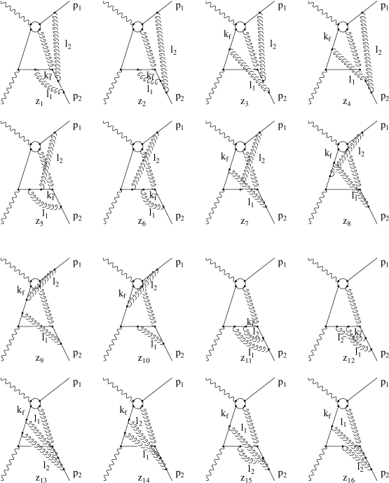
Figure 5: The Abelian diagrams of the topology C.

Group 1.

We start with group 1. The amplitudes $z_{1}$ and $z_{3}$ may be written as

$$z_{1}=\int\frac{dk_{f}}{(2\pi)^{4}}\int\frac{dl_{1}}{(2\pi)^{4}}\Big{[}e\kern-6.0pt/\frac{i}{/\kern-6.0ptk_{\bar{f}}+/\kern-4.0ptl_{1}-m_{q}+i0}i\gamma^{\mu}\Big{]}M^{(1)}_{\mu}$$ (61)

$$z_{3}=\int\frac{dk_{f}}{(2\pi)^{4}}\int\frac{dl_{1}}{(2\pi)^{4}}\Big{[}i\gamma^{\mu}\frac{i}{/\kern-6.0ptk_{f}-/\kern-4.0ptl_{1}-m_{q}+i0}e\kern-6.0pt/\Big{]}M^{(1)}_{\mu}$$ (62)

where $M^{(1)}_{\mu}$ is some one loop sub-diagram, which is identical in both $z_{1}$ and $z_{3}$. Such a representation of the diagrams is very convenient because it turns out that the cancellation of double logarithmic contributions could be traced without explicit computations of the separate diagrams. Instead we observe the cancellations by comparing diagrams in some subgroups and using kinematic simplifications specific to the double logarithmic approximation.

Because the final quark line is hard we might write $M^{(1)}_{\mu}=p_{2\mu}M^{1}$. The momenta $l_{1}$ must be softer than $k_{\bar{f}}$, otherwise no double logarithms can appear. Then we find that integrand of the diagram $z_{1}$ contains $(p_{2}\cdot k_{\bar{f}})$. Therefore decomposing the momenta $(k_{\bar{f}})$ into $k_{f}$ and $p_{2}$ we find that only the component parallel to $k_{f}$ contributes. We remind the reader that $p_{2}^{2}=m^{2}_{q}\to 0$. Introducing $n_{\mu}$, the unit vector parallel to $k_{f}$,

$$n^{\mu}=\frac{k_{f}^{\mu}}{|k_{f}|},$$ (63)

we obtain for the sum of the diagrams

$$z_{1}+z_{3}=-\int\frac{dk_{f}}{(2\pi)^{4}}\int\frac{dl_{1}}{(2\pi)^{4}}e\kern-6.0pt/M^{1}(n\cdot p_{2})\Big{[}\frac{1}{nl_{1}+i0}+\frac{1}{-nl_{1}+i0}\Big{]}M^{1}=0$$ (64)

Thus the leading contribution in the integrand, responsible for the double logarithmic asymptotic, cancels. This is shown in Fig. 3.

As we will see below the mechanism of the cancellation is very general and is related to the dipole mechanism. Indeed we may define an impact factor as a sub-diagram, where a real photon produces a nearly on-shell quark and antiquark, which interacts with the soft gluons. The remarkable fact is that in the configuration responsible for double logarithms both particles move in the same direction. Because the quark momenta is harder than the gluon momenta, only the direction of its movement plays a role.

$$\frac{k_{\bar{f}}p}{k_{\bar{f}}l}=\frac{np}{nl}.$$

Further, because the $b\bar{b}$ system does not have a net color charge, being produced by a photon, the first term in the multi-pole expansion of interaction of this system with any number of soft gluons is the color-dipole moment. This leads to the power suppression of the sub-diagram and the loss of the double logarithms.

Group 2.
We continue with group 2 which constitutes diagrams $z_{2}$ and $z_{4}$. The corresponding amplitudes could be written as

$$z_{2}=\int\frac{dk_{f}}{(2\pi)^{4}}\int\frac{dl_{1}}{(2\pi)^{4}}\Big{[}e\kern-6.0pt/\frac{i}{/\kern-6.0ptk_{\bar{f}}+/\kern-4.0ptl_{1}-m_{q}+i0}i\gamma^{\mu}\Big{]}M^{(2)}_{\mu}$$ (65)

$$z_{4}=\int\frac{dk_{f}}{(2\pi)^{4}}\int\frac{dl_{1}}{(2\pi)^{4}}\Big{[}i\gamma^{\mu}\frac{i}{/\kern-6.0ptk_{f}-/\kern-4.0ptl_{1}-m_{q}+i0}e\kern-6.0pt/\Big{]}M^{(2)}_{\mu}$$ (66)

where as before, $M^{(2)}_{\mu}$ is some sub-diagram,and we may write $M^{(2)}_{\mu}=p_{2\mu}M^{2}$. Again, the momenta $l_{1}$ is softer than $k_{\bar{f}}$ and only the component of $k_{\bar{f}}$ parallel to $k_{f}$ contributes. We have

$$z_{2}+z_{4}=-\int\frac{dk_{f}}{(2\pi)^{4}}\int\frac{dl_{1}}{(2\pi)^{4}}e\kern-6.0pt/M^{(2)}(n\cdot p_{2})\Big{[}\frac{1}{nl_{1}+i0}+\frac{1}{-nl_{1}+i0}\Big{]}M^{2}=0$$ (67)

We thus see that the leading contribution to the integrand, which gives rise to the double logarithmic asymptotic, cancels.

Group 3.
We turn now to the amplitudes for the diagrams $z_{5},z_{6},z_{7}$ which may be written as

$$z_{5}=\int\frac{dk_{f}}{(2\pi)^{4}}\int\frac{dl_{1}}{(2\pi)^{4}}\int\frac{dl_{2}}{(2\pi)^{4}}\Big{[}e\kern-6.0pt/\frac{i}{/\kern-6.0ptk_{\bar{f}}+/\kern-4.0ptl_{1}+/\kern-4.0ptl_{2}-m_{q}+i0}i\gamma^{\mu}\frac{i}{/\kern-6.0ptk_{\bar{f}}+/\kern-4.0ptl_{2}-m_{q}+i0}i\gamma^{\nu}\Big{]}M^{(5)}_{\mu,\nu}$$ (68)

$$z_{6}=\int\frac{dk_{f}}{(2\pi)^{4}}\int\frac{dl_{1}}{(2\pi)^{4}}\int\frac{dl_{2}}{(2\pi)^{4}}\Big{[}e\kern-6.0pt/\frac{i}{/\kern-6.0ptk_{\bar{f}}+/\kern-4.0ptl_{1}+/\kern-4.0ptl_{2}-m_{q}+i0}i\gamma^{\nu}\frac{i}{/\kern-6.0ptk_{\bar{f}}+/\kern-4.0ptl_{1}-m_{q}+i0}i\gamma^{\mu}\Big{]}M^{(6)}_{\mu,\nu}$$ (69)

$$z_{7}=\int\frac{dk_{f}}{(2\pi)^{4}}\int\frac{dl_{1}}{(2\pi)^{4}}\int\frac{dl_{2}}{(2\pi)^{4}}\Big{[}i\gamma^{\mu}\frac{i}{/\kern-6.0ptk_{f}-/\kern-4.0ptl_{1}-m_{q}+i0}e\kern-6.0pt/\frac{i}{/\kern-6.0ptk_{\bar{f}}+/\kern-4.0ptl_{2}-m_{q}+i0}i\gamma^{\nu}\Big{]}M^{(7)}_{\mu,\nu}$$ (70)

it is clear from the diagrams that we can write to the accuracy needed for the relevant subgraphs, $M^{(5)}_{\mu,\nu}=M^{(6)}_{\mu,\nu}=M^{(7)}_{\mu,\nu}=p_{2\mu}p_{1\nu}M^{3}$. The momenta $l_{1},l_{2}$ are softer than $k_{\bar{f}}$ and only the component of $k_{\bar{f}}$ parallel to $k_{f}$ contributes. After simplifications, we obtain

$$z_{5}+z_{6}+z_{7} = \int\frac{dk_{f}}{(2\pi)^{4}}\int\frac{dl_{1}}{(2\pi)^{4}}\int\frac{dl_{2}}{(2\pi)^{4}}e\kern-6.0pt/M^{3}(n\cdot p_{2})(n\cdot p_{1})$$

$$\Big{[} \frac{1}{n(l_{1}+l_{2})}\frac{1}{(nl_{2})}+\frac{1}{n(l_{1}+l_{2})}\frac{1}{(nl_{1})}-\frac{1}{(nl_{1})}\frac{1}{(nl_{2})}\Big{]}=0$$

Again, we see that the leading contribution to the integrand, which could give rise to the double logarithmic asymptotic, cancels.

Figure 6: The general mechanism of the DL cancellation in the groups 3-6 is the dipole interaction of a collinear pair of quarks with two soft gluons.

Group 4.
The amplitudes for $z_{8},z_{9},z_{10}$ could be written as

$$z_{8}=\int\frac{dk_{f}}{(2\pi)^{4}}\int\frac{dl_{1}}{(2\pi)^{4}}\int\frac{dl_{2}}{(2\pi)^{4}}\Big{[}i\gamma^{\mu}\frac{i}{/\kern-6.0ptk_{f}-/\kern-4.0ptl_{1}-m_{q}+i0}i\gamma^{\nu}\frac{i}{/\kern-6.0ptk_{f}-/\kern-4.0ptl_{1}-/\kern-4.0ptl_{2}-m_{q}+i0}e\kern-6.0pt/\Big{]}M^{(8)}_{\mu,\nu}$$ (72)

$$z_{9}=\int\frac{dk_{f}}{(2\pi)^{4}}\int\frac{dl_{1}}{(2\pi)^{4}}\int\frac{dl_{2}}{(2\pi)^{4}}\Big{[}i\gamma^{\nu}\frac{i}{/\kern-6.0ptk_{f}-/\kern-4.0ptl_{2}-m_{q}+i0}i\gamma^{\mu}\frac{i}{/\kern-6.0ptk_{f}-/\kern-4.0ptl_{1}-/\kern-4.0ptl_{2}-m_{q}+i0}e\kern-6.0pt/\Big{]}M^{(9)}_{\mu,\nu}$$ (73)

$$z_{10}=\int\frac{dk_{f}}{(2\pi)^{4}}\int\frac{dl_{1}}{(2\pi)^{4}}\int\frac{dl_{2}}{(2\pi)^{4}}\Big{[}i\gamma^{\nu}\frac{i}{/\kern-6.0ptk_{f}-/\kern-4.0ptl_{2}-m_{q}+i0}e\kern-6.0pt/\frac{i}{/\kern-6.0ptk_{\bar{f}}+/\kern-4.0ptl_{1}-m_{q}+i0}i\gamma_{\mu}\Big{]}M^{(10)}_{\mu,\nu}$$ (74)

with $M^{(8)}_{\mu,\nu}=M^{(9)}_{\mu,\nu}=M^{(10)}_{\mu,\nu}=p_{2\mu}p_{1\nu}M^{4}$ to the desired accuracy for the sub-diagrams. The momenta $l_{1},l_{2}$ are softer than $k_{\bar{f}}$ and only the component of $k_{\bar{f}}$ parallel to $k_{f}$ contributes. After simplifications, we obtain

$$z_{8}+z_{9}+z_{10} = \int\frac{dk_{f}}{(2\pi)^{4}}\int\frac{dl_{1}}{(2\pi)^{4}}\int\frac{dl_{2}}{(2\pi)^{4}}e\kern-6.0pt/M^{4}(n\cdot p_{2})(n\cdot p_{1})$$

$$\Big{[} -\frac{1}{(nl_{1})}\frac{1}{(nl_{2})}+\frac{1}{n(l_{1}+l_{2})}\frac{1}{(nl_{2})}+\frac{1}{n(l_{1}+l_{2})}\frac{1}{(nl_{1})}\Big{]}=0$$

We see that the leading contribution to the integrand cancels. The mechanism of the cancellation is identical to the one of group 3. It is important to note specially for purposes of the next section that $M^{4}=M^{3}$. Hence one might find another 2 sets of 3 diagrams in groups 3 and 4, which cancel in groups of three.

Group 5.
The amplitudes for $z_{11},z_{12},z_{15}$ could be written as

$$z_{15}=\int\frac{dk_{f}}{(2\pi)^{4}}\int\frac{dl_{1}}{(2\pi)^{4}}\int\frac{dl_{2}}{(2\pi)^{4}}\Big{[}i\gamma^{\mu}\frac{i}{/\kern-6.0ptk_{f}-/\kern-4.0ptl_{1}-m_{q}+i0}e\kern-6.0pt/\frac{i}{/\kern-6.0ptk_{\bar{f}}+/\kern-4.0ptl_{2}-m_{q}+i0}i\gamma^{\nu}\Big{]}M^{(15)}_{\mu,\nu}$$ (76)

$$z_{12}=\int\frac{dk_{f}}{(2\pi)^{4}}\int\frac{dl_{1}}{(2\pi)^{4}}\int\frac{dl_{2}}{(2\pi)^{4}}\Big{[}e\kern-6.0pt/\frac{i}{/\kern-6.0ptk_{\bar{f}}+/\kern-4.0ptl_{1}+/\kern-4.0ptl_{2}-m_{q}+i0}i\gamma^{\mu}\frac{i}{/\kern-6.0ptk_{\bar{f}}+/\kern-4.0ptl_{2}-m_{q}+i0}i\gamma^{\nu}\Big{]}M^{(12)}_{\mu,\nu}$$ (77)

$$z_{11}=\int\frac{dk_{f}}{(2\pi)^{4}}\int\frac{dl_{1}}{(2\pi)^{4}}\int\frac{dl_{2}}{(2\pi)^{4}}\Big{[}e\kern-6.0pt/\frac{i}{/\kern-6.0ptk_{\bar{f}}+/\kern-4.0ptl_{1}+/\kern-4.0ptl_{2}-m_{q}+i0}i\gamma^{\nu}\frac{i}{/\kern-6.0ptk_{\bar{f}}+/\kern-4.0ptl_{1}-m_{q}+i0}i\gamma^{\nu}\Big{]}M^{(11)}_{\mu,\nu}$$ (78)

with $M^{(11)}_{\mu,\nu}=M^{(12)}_{\mu,\nu}=M^{(15)}_{\mu,\nu}=p_{1\mu}p_{1\nu}M^{5}$ the relevant sub-diagrams. The momenta $l_{1},l_{2}$ have to be softer than $k_{\bar{f}}$ and only component of $k_{\bar{f}}$ parallel to $k_{f}$ contributes. After simplifications, we obtain

$$z_{11}+z_{12}+z_{15} = \int\frac{dk_{f}}{(2\pi)^{4}}\int\frac{dl_{1}}{(2\pi)^{4}}\int\frac{dl_{2}}{(2\pi)^{4}}e\kern-6.0pt/M^{5}(n\cdot p_{1})(n\cdot p_{1})$$

$$\Big{[} -\frac{1}{(nl_{1})}\frac{1}{(nl_{2})}+\frac{1}{n(l_{1}+l_{2})}\frac{1}{(nl_{2})}+\frac{1}{n(l_{1}+l_{2})}\frac{1}{(nl_{1})}\Big{]}=0$$

We again observe the cancellation of the leading contribution to the integrand. The mechanism of cancellation is identical to the one of group 3 and is the just the dipole mechanism.

Group 6.
Finally the amplitudes for $z_{13},z_{14},z_{16}$ could be written as

$$z_{16}=\int\frac{dk_{f}}{(2\pi)^{4}}\int\frac{dl_{1}}{(2\pi)^{4}}\int\frac{dl_{2}}{(2\pi)^{4}}\Big{[}i\gamma^{\mu}\frac{i}{/\kern-6.0ptk_{f}-/\kern-4.0ptl_{1}-m_{q}+i0}e\kern-6.0pt/\frac{i}{/\kern-6.0ptk_{\bar{f}}+/\kern-4.0ptl_{2}-m_{q}+i0}i\gamma^{\nu}\Big{]}M^{(16)}_{\mu,\nu}$$ (80)

$$z_{14}=\int\frac{dk_{f}}{(2\pi)^{4}}\int\frac{dl_{1}}{(2\pi)^{4}}\int\frac{dl_{2}}{(2\pi)^{4}}\Big{[}i\gamma^{\mu}\frac{i}{/\kern-6.0ptk_{f}-/\kern-4.0ptl_{2}-m_{q}+i0}i\gamma^{\nu}\frac{i}{/\kern-6.0ptk_{f}-/\kern-4.0ptl_{1}-/\kern-4.0ptl_{2}-m_{q}+i0}e\kern-6.0pt/\Big{]}M^{(14)}_{\mu,\nu}$$ (81)

$$z_{13}=\int\frac{dk_{f}}{(2\pi)^{4}}\int\frac{dl_{1}}{(2\pi)^{4}}\int\frac{dl_{2}}{(2\pi)^{4}}\Big{[}i\gamma^{\nu}\frac{i}{/\kern-6.0ptk_{f}-/\kern-4.0ptl_{1}-m_{q}+i0}i\gamma^{\mu}\frac{i}{/\kern-6.0ptk_{f}-/\kern-4.0ptl_{1}-/\kern-4.0ptl_{2}-m_{q}+i0}e\kern-6.0pt/\Big{]}M^{(13)}_{\mu,\nu}$$ (82)

where as before we write to this accuracy, $M^{(13)}_{\mu,\nu}=M^{(14)}_{\mu,\nu}=M^{(16)}_{\mu,\nu}=p_{1\mu}p_{1\nu}M^{6}$. The momenta $l_{1},l_{2}$ have to be softer than $k_{\bar{f}}$ and only the component of $k_{\bar{f}}$ parallel to $k_{f}$ contributes. After simplifications, we obtain

$$z_{13}+z_{14}+z_{16} = \int\frac{dk_{f}}{(2\pi)^{4}}\int\frac{dl_{1}}{(2\pi)^{4}}\int\frac{dl_{2}}{(2\pi)^{4}}e\kern-6.0pt/M^{6}(n\cdot p_{1})(n\cdot p_{1})$$

$$\Big{[} -\frac{1}{(nl_{1})}\frac{1}{(nl_{2})}+\frac{1}{n(l_{1}+l_{2})}\frac{1}{(nl_{2})}+\frac{1}{n(l_{1}+l_{2})}\frac{1}{(nl_{1})}\Big{]}=0$$

which explicitly shows the cancellation of the leading terms. The mechanism of the cancellation is identical to the one for the earlier groups and is the dipole mechanism. Note that for these two groups as well, $M^{5}=M^{6}$ after interchanging $l_{1}$ and $l_{2}$. Hence one might expect to find another two sets of three diagrams in groups 5 and 6, which cancel in groups of three.

In conclusion, we have shown that all diagrams $z_{1}-z_{16}$ cancel in group of two or three due to the dipole mechanism.

3.3 Inclusion of non-abelian diagrams

The inclusion of the non-abelian contributions do not pose any new difficulties. In fact, there are many simplifications because the final state quark and antiquark are produced by photons and hence carry no net color charge. When the color factors are included the cancellations take place between diagrams with the same such factors. For example, consider the cancellation between the diagrams of group 1. Here $z_{1}$ and $z_{3}$ have the same group factor since the only difference between them is an abelian vertex. The same is true for group 2. Thus the cancellation between the diagrams of groups 1 and 2 proceed as in the previous section even in the full non-abelian theory.

Consider next, group 3 of the previous subsection. For this case we will discuss the cancellation in two different ways. In the first method we note that only the group theory factor for the diagram $z_{6}$ is different from that of $z_{5}$ and $z_{7}$. Explicitly, for $z_{6}$ the factor is $T_{a}T_{c}T_{a}T_{b}T_{c}T_{b}$ while for the other two it is $T_{a}T_{c}T_{b}T_{a}T_{c}T_{b}$. All other factors are the same as in the previous section with the rule that the group factors are overall multiplicative. In particular, the sub-diagrams $M^{(5)}_{\mu,\nu}=M^{(6)}_{\mu,\nu}=M^{(7)}_{\mu,\nu}=p_{2\mu}p_{1\nu}M^{3}$ contain no color matrices. Now we can write the color factor of $z_{6}$ as the one for $z_{5}$ and $z_{7}$ plus a left over term which is $if_{abc}T_{a}T_{c}T_{b}(C_{F}-C_{A}/2)$. Consider now the diagrams in group 4 of the previous section. Here the group factor associated with $z_{8}$ is $T_{a}T_{c}T_{b}T_{a}T_{c}T_{b}$ which is different from $z_{9}$ and $z_{10}$ which is $T_{a}T_{c}T_{a}T_{b}T_{c}T_{b}$. The difference now is $-if_{abc}T_{a}T_{c}T_{b}(C_{F}-C_{A}/2)$. Using the fact that $M^{3}=M^{4}$ we see that the left over pieces from groups 3 and 4 cancel each other out. It is easy to check that the same applies to the combination of groups 5 and 6.

It is clear from the above discussion, that it is much more straightforward in the non abelian case to change the assignment of the diagrams into different groups. It is easy to see that apart from the group theory factors, and in the soft approximation, the diagrammatic expressions for $z_{6}$ and $z_{8}$ of the previous subsection (from groups 3 and 4) are the same (using of course $M^{3}=M^{4}$). From groups 5 and 6 of the previous subsection the same applies to the expressions for $z_{12}$ and $z_{14}$ (in this case using $M^{5}=M^{6}$). Thus the following assignment of the diagrams in the non-abelian case into different groups will make sure that all diagrams in a group have the same group theoretical factors:

1. $z_{1}+z_{3}=0$

2. $z_{2}+z_{4}=0$

3. $z_{5}+z_{8}+z_{7}=0$

4. $z_{6}+z_{9}+z_{10}=0$

5. $z_{11}+z_{14}+z_{15}=0$

6. $z_{13}+z_{12}+z_{16}=0$

The new assignment does not change the results for the abelian case and now the cancellation in the non-abelian case proceeds within each group. The only non-trivial result one must use is the equalities $M^{3}=M^{4}$ and $M^{5}=M^{6}$. These are always seen to be true in the soft approximation. In the present grouping, the diagrams in each group are seen to be related to each other by a cyclic permutation of the gluon lines. Such a cyclic permutation leaves the color factor unchanged.

The cancellation between the other non Abelian diagrams shown in Fig.7 also proceeds similarly: For example, $z_{21}$ cancels $z_{22}$; $z_{23}$ cancels $z_{24}$ and so on.

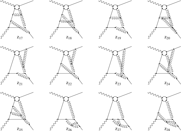
Figure 7: Non-Abelian diagrams.

This discussion now has been set up for generalization to all orders.

3.4 Generalization to higher orders

We see that the cancellation at the 3 loop level discussed in the previous subsection relies on the following: (1) the soft approximation,(2) algebraic identities like

$${1\over-p\cdot k_{1}}+{1\over p\cdot k_{1}}=0$$ (84)

$${1\over-p\cdot k_{1}}{1\over-p\cdot(k_{1}+k_{2})}+{1\over p\cdot k_{1}}{1\over-p\cdot k_{2}}+{1\over p\cdot(k_{1}+k_{2})}{1\over p\cdot k_{2}}=0,$$

and that diagrams in the same group are related by a cyclic permutation of the gluon lines. In the above, $p$ is a generic hard momentum and $k_{i}$ are the soft ones. The soft approximation essentially tells us that a soft gluon does not see spin and more explicitly if $p$ generically denotes a hard fermion momentum then we can consistently use,${i\over 2p\cdot k}$ for the hard propagator and $2p^{\mu}$ for the vertex factors. This will ensure the equalities like $M^{3}=M^{4}$ needed for the cancellations to occur for our process. As far as the algebraic identities are concerned, they are in fact special cases of the Sterman-Libby identities [18]. These identities obtained by considering diagrams related by cyclic permutations of the gluon lines read in general:

$$\sum_{m=0}^{n}\prod_{i=0}^{m-1}{1\over p\cdot q_{m}-p\cdot q_{i}}\prod_{j=m+1}^{n}{1\over p\cdot q_{m}-p\cdot q_{j}}=0$$ (85)

In the above, $q_{i}\equiv k_{1}+k_{2}+.....+k_{i}$ and $q_{i=0}\equiv 0$. These identities are easily seen to reduce to Eqs.(84) for the cases $n=1,2$. Thus we see each of the technical ingredients have a generalization to higher loop orders. The physics of the dipole mechanism and the color singlet nature of the final (and initial) states combined with the above guarantee the cancellations needed to all orders.

Figure 8: The general mechanism of the DL cancellation is the dipole interaction of a collinear pair of quarks with many soft gluons.

4 Contributing diagrams at the next-to-leading logarithmic order

The goal of this section is to identify those diagrams that either vanish or cancel some other diagrams at next-to-leading logarithmic order. The diagrams left over are then just those needed in the discussion in Section 2.3. Our explicit analysis is only at the two loop level and at the end we argue that the results hold to NLL accuracy. In the first subsection, we discuss the regime contributing to the next-to-leading logarithms. We then introduce a power counting technique that enables us to discover the non-vanishing diagrams and make appropriate approximations. Armed with these two techniques, we are able to exclude a set of diagrams without actually carrying out the loop integrations. We remind the reader that we work throughout in the Feynman gauge. In this gauge we will see that for the process under consideration, the additional logarithms at the NLL level must be of collinear origin.

4.1 Sources of single logarithms

In a two-particle scattering process, all momenta lie in the same plane. We can take two of the independent momenta, $k_{1}$ and $k_{2}$, as ’+’ and ’-’ direction, and denote the third momentum as $p$ ($p$ could be either $p_{1}$ or $p_{2}$). The loop momentum $l$ can be expressed in terms of light cone variables

$$l=\alpha k_{1}+\beta k_{2}+l_{\perp}.$$ (86)

We note that the following integral in the soft regime

$$\int d\alpha d\beta\frac{1}{\alpha^{i}}\frac{1}{\beta^{j}}\Theta(s\alpha\beta-m^{2}),i,j=...,-2,-1,0,1,2,...,$$ (87)

gives terms like $\log^{2}\frac{s}{m^{2}}$, $(\frac{m^{2}}{s})^{n}\log\frac{s}{m^{2}}$ or $(\frac{m^{2}}{s})^{n}$. In other words, the soft regime cannot give rise to a single logarithm at the one-loop level.

Consider an n-loop Feynman integral with loop momenta $l_{i},1\leq i\leq n$. We can decompose $l_{i}$ in terms of ’external momenta’ $k_{1}$ and $k_{2}$,

$$l_{i}=\alpha_{i}k_{1}+\beta_{i}k_{2}+l_{i\perp}.$$ (88)

In the soft region, $|\alpha_{i}|,|\beta_{i}|,\frac{|l_{i\perp}^{2}|}{s}\ll 1$, the Feynman integral does not give the next-to-leading logarithm, $\log^{2n-1}\frac{m^{2}}{s}$. This is because, intuitively, each integration over the light cone variables $\alpha$ and $\beta$ gives either a logarithm or a power suppression, as exemplified in the previous paragraph. We now prove this statement more rigorously.

We first note the following replacement for loop momenta corresponding to a soft line,

$$\frac{1}{l_{i}^{2}-m_{i}^{2}+i\epsilon}\rightarrow-i\pi\delta(s\alpha_{i}\beta_{i}+l_{i\perp}^{2}-m_{i}^{2}).$$ (89)

The rest of the propagators can be categorized into hard, collinear and soft ones. The hard propagators are irrelevant to the infrared sensitivity. The remaining possibilities are collinear to $k_{1}$ or $k_{2}$, soft or collinear to $p$. We discuss them in turn.

(1) Collinear to $k_{1}$ or $k_{2}$. A boson that is parallel to $k_{1}$ has a propagator that can be written as

$$\frac{1}{(k_{1}+\sum_{i}u_{i}l_{i})^{2}} = \frac{1}{(1+\sum_{i}u_{i}\alpha_{i})(\sum_{i}u_{i}\beta_{i})s/2}$$ (90)

$$\rightarrow \frac{2}{s}\frac{1}{\sum_{i}u_{i}\beta_{i}}.$$

The fermionic propagator can be expressed as

$$\frac{1}{(/\kern-6.0ptk_{1}+\sum_{i}u_{i}/\kern-4.0ptl_{i})-m} = \frac{(/\kern-6.0ptk_{1}+\sum_{i}u_{i}/\kern-4.0ptl_{i})-m}{(k_{1}+\sum_{i}u_{i}l_{i})^{2}-m^{2}}$$ (91)

$$\rightarrow \frac{/\kern-6.0ptk_{1}}{(\sum_{i}u_{i}\beta_{i})s/2}$$

(2) Soft. A bosonic propagator

$$\frac{1}{(\sum_{i}u_{i}l_{i})^{2}}=\frac{1}{(\sum_{i}u_{i}\alpha_{i})(\sum_{i}u_{i}\beta_{i})s+(\sum_{i}u_{i}l_{i\perp})^{2}}$$ (92)

Using $\delta(s\alpha_{i}\beta_{i}+l_{i\perp}^{2}-m_{i}^{2})$, and $2\sqrt{(\alpha_{i}\beta_{j})(\alpha_{j}\beta_{i})}\leq\alpha_{i}\beta_{j}+\alpha_{j}\beta_{i}$, it is easy to show

$$|(\sum_{i}u_{i}\alpha_{i})(\sum_{i}u_{i}\beta_{i})s|>(\sum_{i}u_{i}l_{i\perp})^{2}.$$ (93)

Hence, the expansion below,

$$\frac{1}{(\sum_{i}u_{i}\alpha_{i})(\sum_{i}u_{i}\beta_{i})s}\left[1-\frac{(\sum_{i}u_{i}l_{i\perp})^{2}}{(\sum_{i}u_{i}\alpha_{i})(\sum_{i}u_{i}\beta_{i})s}-\cdots\right],$$ (94)

converges. The fermionic propagator has a term proportional to $l_{i}^{\mu}$, in addition to the expansion above.

(3) Collinear to $p$. Again, the bosonic propagator can be expanded as

$$\frac{1}{(p+\sum_{i}u_{i}l_{i})^{2}-m_{i}^{2}} \rightarrow \frac{1}{\sum_{i}u_{i}(\alpha_{i}+\beta_{i})|t|/2+\sum_{i}u_{i}(p_{\perp}\cdot l_{i\perp})}$$ (95)

$$= \frac{1}{\sum_{i}u_{i}(\alpha_{i}+\beta_{i})|t|/2}\left[1-\frac{\sum_{i}u_{i}(p_{\perp}\cdot l_{i\perp})}{\sum_{i}u_{i}(\alpha_{i}+\beta_{i})|t|/2}-\cdots\right]$$

The fermionic propagator may give rise to an additional $l_{i}^{mu}$ in the numerator.

First, we only include the first term in the series in eq.(94, 95) and apply the following trick

$$\frac{1}{\alpha}\frac{1}{\beta}\frac{1}{\alpha+\beta}=\left(\frac{1}{\alpha}-\frac{1}{\alpha+\beta}\right)\frac{1}{\beta^{2}}.$$ (96)

This trick reduces the number of different combinations of $\alpha$’s and $\beta$’s while splitting one term into two.

Therefore, when the propagators in case (1) and only the first terms in the expansions of the soft and collinear-to-$p$ propagators are included, the integral can be reduced to a finite sum of the type

$$\int_{\mathrm{soft\ regime}}\prod_{i}^{2n}d\sigma_{i}\frac{1}{\sigma^{m_{i}}},$$ (97)

where $\sigma$’s represent $\alpha$’s, $\beta$’s or the combinations thereof. It is evident that an integration over each $\sigma$ gives either a logarithm or a power suppression $m^{2}/s$. No next-to-leading logarithm can arise in the soft regime.

We now include the whole series in eq.(94, 95), as well as their fermionic counterpart whenever appropriate. The denominators are polynomials of $\alpha_{i}$ and $\beta_{i}$,

$$\frac{1}{\sum_{i}u_{i}\alpha_{i}},\frac{1}{\sum_{i}u_{i}\beta_{i}},\frac{1}{\sum_{i}u_{i}(\alpha_{i}+\beta_{i})}$$ (98)

The numerators consists of terms proportional to $p^{\mu}$ and $l_{i}^{\nu}$. The Feynman integral is thus of the following form

$$\int\prod d\alpha_{i}d\beta_{i}d^{2}l_{i\perp}\frac{\bar{f_{1}}(\alpha_{i},\beta_{i},p_{\perp}\cdot l_{i\perp},l_{i\perp}\cdot l_{j\perp})\prod l_{j\perp}^{\mu_{j}}}{\bar{f_{2}}(\alpha_{i},\beta_{i})},$$ (99)

where $\bar{f_{1}}$ and $\bar{f_{2}}$ are both polynomial functions of their arguments and the spinor structure is not interesting. Since $p_{\perp}$ is the only vector in the integrand which is not the integration variable, the integral of interest can further be reduced to

$$\int\prod d\alpha_{i}d\beta_{i}d^{2}l_{i\perp}\frac{\bar{f_{1}}(\alpha_{i},\beta_{i},p_{\perp}\cdot l_{i\perp},l_{i\perp}\cdot l_{j\perp})}{\bar{f_{2}}(\alpha_{i},\beta_{i})},$$ (100)

where we have further left out the tensorial structure of $p_{\perp}^{\mu}$ and $g^{\mu\nu}$.

By noting

$$l_{i\perp}\cdot l_{j\perp} = \sqrt{l_{i\perp}^{2}}\sqrt{l_{j\perp}^{2}}\cos(\theta_{i}-\theta_{j})$$

$$p_{\perp}\cdot l_{i\perp} = \sqrt{p_{\perp}^{2}}\sqrt{l_{i\perp}^{2}}\cos\theta_{i}$$ (101)

where the angles $\theta_{i}$ are relative to the vector $\vec{p_{\perp}}$, the integral can be cast into

$$\int\prod d\alpha_{i}d\beta_{i}dl_{i\perp}^{2}\frac{f_{1}(\alpha_{i},\beta_{i},p_{\perp}\cdot l_{i\perp},l_{i\perp}\cdot l_{j\perp})}{f_{2}(\alpha_{i},\beta_{i})}\int\prod d\theta_{i}f_{3}(\theta).$$

$$\rightarrow \int\prod d\alpha_{i}d\beta_{i}\sum\frac{P(\sqrt{\alpha_{i}},\sqrt{\beta_{i}},\sqrt{\sum(u_{i}\alpha_{i}+v_{j}\beta_{j})})}{Q(\alpha_{i},\beta_{i})}$$ (102)

where $\bar{P}$ and $\bar{Q}$ are polynomial functions of their arguments. We have used the $\delta$ function (eq.(89)) to perform the integration over $l_{i\perp}^{2}$ and implicitly included the resulting $\Theta$ functions in the ’polynomials’ $\bar{P}$. The summation in the second line is due to the expansions in the soft and collinear-to-$p$ propagators. It is a convergent series.

Now we examine the arguments of the polynomial $\bar{P}$ in eq.(102). The $\sqrt{\sum(u_{i}\alpha_{i}+v_{j}\beta_{j})}$ represents various combinations of $\alpha_{i}$ and $\beta_{j}$ that may appear. For such a combination, we split the integration region

$$\sqrt{\alpha_{i}+\beta_{j}}=\left\{\begin{array}[]{ll}\sqrt{\alpha_{i}}\left(1+\frac{1}{2}\frac{\beta_{j}}{\alpha_{i}}+\cdots\right),&\alpha_{i}>\beta_{j}\\ \sqrt{\beta_{j}}\left(1+\frac{1}{2}\frac{\alpha_{i}}{\beta_{j}}+\cdots\right),&\alpha_{i}<\beta_{j}\end{array}\right.$$ (103)

After such maniputions, we obtain a convergent series

$$\int\prod d\alpha_{i}d\beta_{i}\sum\frac{P(\sqrt{\alpha_{i}},\sqrt{\beta_{i}})}{Q(\alpha_{i},\beta_{i})}$$ (104)

with P and Q polynomial functions of $\sqrt{\alpha_{i}}$ and $\sqrt{\beta_{i}}$. In order to obtain the next-to-leading logarithm, $2n-1$ of the integrations have to give logarithm while the last one gives a constant of order 1. This is impossible for the above integral in the soft region. It follows that at least one of the loop momenta has to be taken out of soft region to correctly reproduce the next to leading logarithmic behavior in the Feynman gauge.

4.2 A power counting technique

In order to identify the regime contributing to the next-to-leading logarithmic order at two-loop level, we consider inserting a gluon into the one-loop box diagram. From the previous subsection, we know the inserted gluon has to be collinear. Therefore, we will consider in turn the three topologies with an additional collinear gluon inserted to each of them.

Throughout the following subsections, we always denote the soft loop momentum by $l$ and that of the collinear gluon by $k$.

We take two momenta $p$ and $\bar{p}$ as the basis to decompose the momentum $k$ of the collinear gluon,

$$k=\alpha p+\beta\bar{p}+k_{\perp}.$$ (105)

The generic momenta $p$ and $\bar{p}$ can be any two of the external momenta $k_{1}$, $k_{2}$, $p_{1}$ and $p_{2}$.

In the so-called collinear region, without loss of generality, we assume $k$ parallel to $p$ such that

$$|\alpha|\sim 1,|\beta|\sim\sqrt{\frac{k_{\perp}^{2}}{s}}\ll 1.$$ (106)

In general, all the propagators in a Feynman diagram can be characterized as hard (off-shell), soft or collinear (to a certain direction). In order to get the next-to-leading logarithm at two-loop level, which is a double logarithm multiplied with a single logarithm, a Feynman diagram has to contain at least four collinear and one soft propagators. Specifically, the double logarithmic form factor arises from a soft virtual particle ’interacting’ with two (nearly) on-shell particles that are flying apart along two different directions. On the other hand, the interaction between two collinearly flying virtual particles gives rise to the single logarithmic form factor.

As a result, whenever we have less than four collinear propagators, we can immediately conclude that the Feynman diagram does not contribute at the next-to-leading logarithmic level. When we have exactly four collinear and a soft propagator, we only keep terms proportional to $\alpha$ in the numerator. The $\beta$ term can be dropped because it cancels a $\beta$ in the denominator and effectively ’removes’ a collinear propagator. An example of such a collinear propagator is

$$\frac{1}{(p+k)^{2}-m^{2}}=\frac{1}{(1+\alpha)\beta(2p\cdot\bar{p})+k_{\perp}^{2}+p^{2}+\bar{p}^{2}-m^{2}}.$$ (107)

And when we carry out the integration over $k$, we can pick up a pole from an ’on-shell’ propagator as the above one. It follows that $\beta s\sim k_{\perp}^{2}$ and $k_{\perp}^{2}$ should also be dropped. If we get more than four collinear propagators, we will keep all the terms. However, in general the terms proportional to $\alpha$ are suppressed by $m^{2}$ and thus leave $\beta$ and $k_{\perp}^{2}$ the leading terms.

4.3 Vertex functions

When inserting a gluon into a box diagram, we will obtain one-loop vertex subdiagrams inside four of the resulting two-loop diagrams. Two of the vertex corrections each have two legs (nearly) on-shell and the other soft. There is no large scale of order $s$, other than that from the UV cutoff, in such a sub-diagram. Therefore, these two vertex functions contain no infrared logarithms.

The other two vertex function subdiagrams have two (nearly) on-shell and one off-shell legs each. They do contribute single logarithms in all the three topologies. Such vertex corrections are shown in Fig.9(g, h), 11(g, h), 12(e, f) and 13(e, f). Self energy corrections are understood and not explicitly drawn.

Hereafter, we will omit the diagrams (and regions of diagram) that give rise to large logarithms only of ultraviolet origin, until we are ready to run the relevant parameters using the RGE.

4.4 Contributing diagrams in topology A

We show some of the diagrams relevant to the next-to-leading logarithms of Topology A in Fig.9. The shorter fermion lines in the box subdiagrams represent the off-shell propagators, which characterize the Topology A. Note Fig.9(a) and (b) represent different regions of the same diagram, where the soft gluons are labeled by $l$ and the collinear gluons by $k$. The same comments apply to Fig.9(c) and (d). (We will follow the conventions that the characteristic off-shell propagator is denoted by the shorter line, $l$ for the soft momentum and $k$ for collinear momentum throughout the rest of this article.)

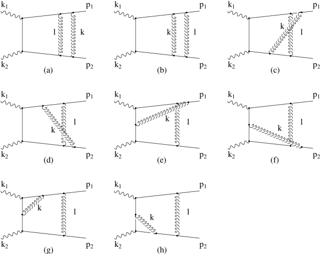
Figure 9: Diagrams relevant to the next-to-leading logarithms in Topology A. The diagrams dependent only on $C_{F}$ are shown here.

The reduced diagram for the first six diagrams, Fig.9(a) through (f), all consist of a hard vertex with four jets attached to it, as shown in Fig.10. The two jets eventually emerge as quark and antiquark further interact with each other via a soft diagram (the gluon with momentum $l$). One of them consists of the collinear gluon and the quark or antiquark. In addition, these subset of diagrams are gauge invariant, since the reciprocal subset (consisting of vertex correction and self-energy subdiagrams) are gauge invariant. We can now invoke results from a general power counting analysis of infrared sensitive contributions (both soft and collinear) to a typical wide-angle scattering process [19, 20]. It was shown there that the logarithmic configuration requires that jet lines are attached to hard vertices by a single line, otherwise there is power suppression. The analysis of [19, 20] was made in a physical gauge, but it obviously holds for the gauge invariant set discussed above. Hence, the sum of Fig.9(a) through (f) does not contain infrared logarithms.

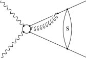
Figure 10: Jet diagram for topology A

The remaining diagrams are Fig.9(b) and (h), which contribute to the next-to-leading logarithmic order. These are just the diagrams proportional only to $C_{F}$ contributing to on-shell Sudakov form factor to NLL accuracy which is extensively discussed in [14]

4.5 Contributing diagrams in topology B

Now we turn to the diagrams in Fig.(11). In Fig.(11e), the collinear gluon, labeled by $k$, can be parallel to $p_{1}$, $k_{1}$ or $k_{2}$. We discuss them in turn.

Figure 11: Diagrams relevant to the next-to-leading logarithms in Topology B. The t-channel diagrams dependent only on $C_{F}$ are shown here.

i) Parallel to $p_{1}$ ($k\|p_{1}$). There are only three collinear propagators left. This region can be excluded by power counting.

ii) Parallel to $k_{1}$ ($k\|k_{1}$). The soft fermion is the one labeled by $l$, while the fermion labeled by $k+l$ is collinear to $k_{1}$. And the fermion with momentum $k+p_{1}$ is off-shell. There are exactly four collinear and one soft propagator left. Hence we only keep the component of $k$ that is parallel to $k_{1}$. The numerator of the diagram here is,

$$N \propto (/\kern-6.0ptk_{1}+/\kern-6.0ptk+/\kern-4.0ptl)\epsilon\kern-6.0pt/(/\kern-6.0ptk_{1})(/\kern-6.0ptk+/\kern-4.0ptl)$$ (108)

$$\propto /\kern-6.0ptk_{1}\epsilon\kern-6.0pt/(/\kern-6.0ptk_{1})/\kern-6.0ptk_{1}=0,$$

which implies a vanishing contribution to the next-to-leading logarithmic order from this region.

iii) The last possible region is $k\|k_{2}$, which vanishes due to the similar reason as in ii).

Therefore, Fig.11(e) vanishes as well as Fig.11(f). Diagrams Fig.11(a) - (d) can be shown to factorize. Take Fig.11(d) as an example, the numerator of the amplitude is

$$N_{16d} = \bar{u}(p_{1})\gamma^{\alpha}(/\kern-6.0ptk_{1}+/\kern-4.0ptl+/\kern-6.0ptk)\gamma^{\mu}(/\kern-6.0ptk_{1}+/\kern-4.0ptl)\epsilon\kern-6.0pt/(k_{1})m\epsilon\kern-6.0pt/(k_{2})(-/\kern-6.0ptk_{2}+/\kern-4.0ptl)\gamma_{\alpha}(-p\kern-5.0pt/_{2}+/\kern-6.0ptk)\gamma_{\mu}v(p_{2})$$ (111)

$$= \left\{\begin{array}[]{ll}\bar{u}(p_{1})\gamma^{\alpha}(/\kern-6.0ptk_{1}+/\kern-4.0ptl)\epsilon\kern-6.0pt/(k_{1})m\epsilon\kern-6.0pt/(k_{2})(-/\kern-6.0ptk_{2}+/\kern-4.0ptl)\gamma_{\alpha}\left[-4p_{2}\cdot(k_{1}+k)\right]v(p_{2}),&k\|k_{1}\\ \bar{u}(p_{1})\gamma^{\alpha}\left[4k_{1}\cdot(-p_{2}+k)\right](/\kern-6.0ptk_{1}+/\kern-4.0ptl)\epsilon\kern-6.0pt/(k_{1})m\epsilon\kern-6.0pt/(k_{2})(-/\kern-6.0ptk_{2}+/\kern-4.0ptl)\gamma_{\alpha}v(p_{2}),&k\|p_{2}\end{array}\right.$$

The factorization is evident now. Similar results hold for the other three diagrams. However, they do not contain any large single logarithms.

The remaining diagrams, Fig.11(g) and (h) are just the ones included in the resummation discussed in Section 2.3 to this order.

4.6 Contributing diagrams in topology C

In topology C, the two-loop s-channel diagrams only proportional to $C_{F}$ are shown in Fig.(12). The regions contributing to the next-to-leading logarithmic approximation for Fig.(12a, b, c) are both the gluons being parallel to $p_{2}$.

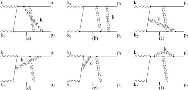
Figure 12: Diagrams relevant to the next-to-leading logarithms in Topology C. The s-channel diagrams dependent only on $C_{F}$ are shown here.

Note the ’incoming’ quark and the ’outgoing’ gluon of the hard subprocess $\gamma q\rightarrow qg$ are nearly on shell. In addition, the gluon labeled by $k$ in the three diagrams are nearly on-shell too. We can expect the contributions only proportional to $C_{F}$ of the three diagrams to cancel to the leading order, in the same manner as discussed earlier in Section 3.

In order to show the cancellation, we decompose

$$k=\alpha_{k}k_{2}+\beta_{k}p_{2}+k_{\perp}.$$ (112)

Each of the three amplitude takes on the form

$$M_{i} = \bar{M_{i}}^{\mu}\frac{1}{-p\kern-5.0pt/_{2}-/\kern-6.0ptk}\gamma_{\mu}v(p_{2})$$

$$= -\bar{M_{i}}^{\mu}\frac{\alpha_{k}/\kern-6.0ptk_{2}+(1+\beta_{k})p\kern-5.0pt/_{2}+/\kern-6.0ptk_{\perp}}{(p_{2}+k)^{2}}\gamma_{\mu}v(p_{2}),$$

with $M_{i}$, $i=1,2,3$, representing amplitudes of Fig.(12a, b, c) respectively. In this subsection, integrations over $l$ and $k$ should be understood in the amplitudes. We consistently omit common numerical factors for simplicity. To the single logarithmic approximation, $\alpha_{k}$ and $k_{\perp}$ terms in the numerators can be neglected. Hence,

$$M_{i} = -\bar{M_{i}}_{\mu}\frac{(1+\beta_{k})p_{2}^{\mu}}{(p_{2}+k)^{2}}v(p_{2})$$

$$= -\frac{1+\beta_{k}}{\beta_{k}}\bar{M_{i}}_{\mu}k^{\mu}\frac{1}{(p_{2}+k)^{2}}v(p_{2})$$

and we have put back the $\alpha_{k}k_{2}+k_{\perp}$ in the second line.

The summation of $k^{\mu}\bar{M_{i}}_{\mu}$ in the three amplitudes closely follows the earlier proof using the Ward Identity (see section 3.1). We obtain (for the piece proportional only to $C_{F}$)

$$M_{1}+M_{2}+M_{3}= -\frac{1+\beta_{k}}{\beta_{k}}[\bar{u}(p_{1})p\kern-5.0pt/_{1}\gamma^{\lambda}\frac{1}{/\kern-6.0ptk_{1}+/\kern-6.0ptk_{2}+/\kern-4.0ptl}\epsilon\kern-6.0pt/(k_{1})\frac{1}{/\kern-6.0ptk_{2}+/\kern-4.0ptl}-\bar{u}(p_{1})\gamma^{\lambda}\frac{1}{/\kern-6.0ptk_{1}+/\kern-6.0ptk_{2}+/\kern-4.0ptl+/\kern-6.0ptk}\epsilon\kern-6.0pt/(k_{1})\frac{1}{/\kern-6.0ptk_{2}+/\kern-6.0ptk+/\kern-4.0ptl}]$$

$$\cdot\epsilon\kern-6.0pt/(k_{2})\frac{1}{/\kern-4.0ptl-m}\gamma_{\lambda}v(p_{2})\frac{1}{(p_{2}+k)^{2}}\frac{1}{k^{2}}\frac{1}{(p_{2}+k+l)^{2}}.$$

The first term is suppressed by the quark mass, while the second one vanishes in the single logarithmic approximation by simple power counting. Therefore, the contributing diagram in Fig.12 are d, e, and f.

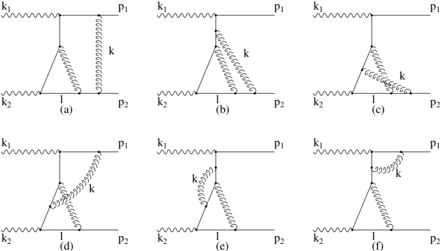
Figure 13: Diagrams relevant to the next-to-leading logarithms in Topology C. The u-channel diagrams dependent only on $C_{F}$ are shown here.

Similarly, the diagrams with the u-channel hard subprocess also include six diagrams. Noteworthy is that Fig.13(a) can also be drawn as a vertex correction to the s-channel diagrams, with the triangle subdiagram being the vertex correction therein. However, we notice they represent different regions. In Fig.13(a), the quark labeled by $l$ is soft, whereas in the s-channel diagram, the corresponding one is collinear to $k_{2}$. A similar remark applies to Fig.13(b). Here, it can be viewed as a vertex correction to the u-channel diagram, which in turn represents a different region. As a summary, the two diagrams shown in Fig.13(a, b) represent the region that both the virtual gluons are parallel to $p_{2}$, while in their counterparts, the two virtual gluons are parallel to $k_{2}$ and $p_{2}$ respectively. Obviously, the sum of Fig.13(a, b, c) vanishes to the next-to-leading logarithmic approximation in exactly the same way Fig.12(a, b, c) do.

Therefore, the contributing diagrams of the Topology C at the two-loop level include Fig.12(d, e, f) and Fig.13(d, e, f) only. We note the diagrams contributing to the “hard” off-shell Sudakov form factor in this topology are mostly non-abelian which are of Sudakov type. Some of these are shown in Fig.14. This completes our argument justifying that the only source of logarithm at this order are of the “Sudakov” type.

Figure 14: Some of the diagrams proportional to $C_{A}$ in topology C.

4.7 Extension to higher loops

In this section, we argue without detailed proof that the above results hold to the full NLL accuracy. We consider only topologies B and C, since topology A, which corresponds to the on-shell Sudakov form factor, has been discussed in detail in [14].

For topologies B and C, consider the insertions of a gluon into the bare diagram. There are two cases:
i) The gluon momentum is in the soft region. The analysis in Section 3 can be applied and it can be factored out.
ii) If the gluon momentum is in collinear region, the analysis in the previous subsections apply and again, factorization results.

All subsequent insertions of gluons in case (ii) must be restricted to the soft region. Therefore, for these the analysis of section 3 apply. In case (i), we keep inserting gluons and apply the same analysis until we encounter a collinear gluon. Then case (ii) applies.

Hence we can conclude that to NLL accuracy, the relevant diagrams are all of the Sudakov type.

5 Summary and Discussions

In this paper we have studied the resummation up to the next to leading logarithmic level of the QCD radiative corrections to $\bar{b}b$ production by photon photon collisions. Apart from the phenomenological applications, this problem has inherent interest in providing a theoretical laboratory to study QCD effects. We showed that to the accuracy considered all logarithms are of the Sudakov type. On a diagram by diagram basis other types of diagrams do give rise to next to leading logarithms but they cancel amongst each other by the dipole mechanism. We explicitly showed how the dipole mechanism works to 3 loops and outlined an all orders generalization. At the NLL level we found that in the Feynman gauge the only new logarithms are of collinear origin. The final expression for the resummed amplitude is given in section 2, eq.(26) together with eq.(41,42,2.3).

6 Acknowledgments

We would like to thank G. Sterman for discussions. This work was supported by the US Department of Energy.

References

• [1] J.F. Gunion, H.E. Haber, G. Kane, and S. Dawson, The Higgs Hunter’s Guide (Addison-Wesley, Reading, MA, 1990).
• [2] J. F. Gunion and H. E. Haber, Phys. Rev. D 48, 5109 (1993).
• [3] K. Hagiwara et al. [Particle Data Group Collaboration], Phys. Rev. D 66, 010001 (2002).
• [4] K. Melnikov and O. Yakovlev, Phys. Lett.  B312, 179 (1993) [hep-ph/9302281].
A. Djouadi, M. Spira, J. J. van der Bij and P. M. Zerwas, Phys. Lett.  B257, 187 (1991).
J. G. Korner, K. Melnikov and O. I. Yakovlev, Phys. Rev.  D53, 3737 (1996) hep-ph/9508334].
K. Melnikov, M. Spira and O. Yakovlev, Z. Phys.  C64, 401 (1994)
• [5] I. F. Ginzburg, G. L. Kotkin, V. G. Serbo and V. I. Telnov, Nucl. Instrum. Meth.  205, 47 (1983).
• [6] V. Telnov, Nucl. Instrum. Meth. A 355, 3 (1995).
• [7] V. S. Fadin, V. A. Khoze and A. D. Martin, Phys. Rev. D 56, 484 (1997) [arXiv:hep-ph/9703402].
• [8] D. L. Borden, V. A. Khoze, W. J. Stirling and J. Ohnemus, Phys. Rev. D 50, 4499 (1994) [arXiv:hep-ph/9405401].
• [9] G. Jikia and A. Tkabladze, Phys. Rev. D 54, 2030 (1996) [arXiv:hep-ph/9601384].
• [10] M. Melles and W. J. Stirling, Phys. Rev. D 59, 094009 (1999) [arXiv:hep-ph/9807332].
• [11] V. V. Sudakov, Sov. Phys. JETP 3, 65 (1956) [Zh. Eksp. Teor. Fiz.  30, 87 (1956)].
• [12] V. G. Gorshkov, V. N. Gribov, L. N. Lipatov and G. V. Frolov, Sov. J. Nucl. Phys.  6, 95 (1968) [Yad. Fiz.  6, 129 (1967)].
• [13] J. Carazzone, E. C. Poggio and H. R. Quinn, Phys. Lett. B 57, 161 (1975).
• [14] J. C. Collins, Adv. Ser. Direct. High Energy Phys.  5, 573 (1989).
• [15] A. V. Smilga, Nucl. Phys. B 161, 449 (1979).
• [16] R. Akhoury, H. Wang and O. I. Yakovlev, Phys. Rev. D 64, 113008 (2001) [arXiv:hep-ph/0102105].
• [17] G. Sterman, An Introduction to Quantum Field Theory, Cambridge University Press, 1993.
• [18] S. B. Libby and G. Sterman, Phys. Rev. D 19, 2468 (1979).
V. Ganapathi and G. Sterman, Phys. Rev. D 23, 2408 (1981).
• [19] R. Akhoury, Phys. Rev. D 19, 1250 (1979).
• [20] G. Sterman, Phys. Rev. D 17, 2773 (1978).