BA-TH/02-451

CERN-TH/2002-352

hep-ph/0212112

Constraints on pre-big bang parameter space
from CMBR anisotropies

V. Bozza^a,b,c, M. Gasperini^d,e, M. Giovannini^c and G. Veneziano^c

^a Dipartimento di Fisica “E. R. Caianiello”, Università di Salerno, 84081 Baronissi, Italy

^b INFN, Sezione di Napoli, Gruppo Collegato di Salerno, Salerno, Italy

^c Theoretical Physics Division, CERN, CH-1211 Geneva 23, Switzerland

^d Dipartimento di Fisica, Università di Bari, Via G. Amendola 173, 70126 Bari, Italy

^e INFN, Sezione di Bari, Bari, Italy

The so-called curvaton mechanism –a way to convert isocurvature perturbations into adiabatic ones– is investigated both analytically and numerically in a pre-big bang scenario where the rôle of the curvaton is played by a sufficiently massive Kalb–Ramond axion of superstring theory. When combined with observations of CMBR anisotropies at large and moderate angular scales, the present analysis allows us to constrain quite considerably the parameter space of the model: in particular, the initial displacement of the axion from the minimum of its potential and the rate of evolution of the compactification volume during pre-big bang inflation. The combination of theoretical and experimental constraints favours a slightly blue spectrum of scalar perturbations, and/or a value of the string scale in the vicinity of the SUSY-GUT scale.

I Introduction

At present, the largest-scale temperature fluctuations of the Cosmic Microwave Background radiation (CMBR) are consistent with a (quasi) scale-invariant spectrum of Gaussian primordial curvature fluctuations [1, 2, 3]. The analysis of the first acoustic oscillations occurring on shorter angular scales adds the information that such curvature fluctuations should be predominantly adiabatic [4, 5, 6, 7]. Although sufficiently small amounts of non-Gaussianity and/or isocurvature perturbations are not excluded, the above-mentioned observational features represent an important constraint for any scenario trying to model the initial stages of our Universe. In a previous Letter [8] we tried to confront the pre-big bang scenario [9, 10, 11] with these constraints. The present paper contains a full description of that analysis and completes it.

Let us recall that, during the pre-big bang phase, the quantum fluctuations of all the light modes present in the low energy effective action are parametrically amplified. Nonetheless, sizeable large-scale adiabatic fluctuations are not easily produced from the initial vacuum through the usual mechanism of parametric amplification. In particular, both tensor and scalar-metric fluctuations are amplified with very steep spectra [12, 13], resulting in adiabatic modes which are far too small to explain the observed level of large-scale CMBR anisotropies [14].

However, not all the primordial spectra of pre-big bang cosmology are blue. For instance, in a pure gravi-dilaton background, the pseudo-scalar supersymmetric partner of the dilaton in the dimensionally-reduced string effective action, the so-called Kalb–Ramond axion, emerges from the pre-big bang phase with a fluctuation spectrum whose tilt depends on the rate of change of the compactification volume [15, 16]. Depending on this, the axion tilt can be negative (red spectrum), positive (blue spectrum), or zero (scale-invariant spectrum). However, since the homogeneous (background) component of the axion is trivial, such a spectrum does not affect directly the metric, hence no curvature perturbation is generated at this primordial level. In other words, the axion perturbations are entropic, isocurvature perturbations. This feature persists, unfortunately, under $S$-duality transformations [15, 16]. If such an axion is massless, or at least light enough not to have decayed yet , the induced CMBR fluctuations on large scales can fit the COBE normalization [17, 18, 19, 20], but, being neither adiabatic nor Gaussian [21], they are not able to fit the observed structure of the first few acoustic peaks.

A possible way out of this problem [8, 10, 22, 23, 24] is offered by the alternative scenario of a massive axion, initially displaced from the minimum of its non-perturbative potential. In that case axion perturbations couple to scalar metric perturbations through the non-vanishing axion’s VEV. Eventually, the axion relaxes toward the minimum of the potential and then, if heavy enough, decays prior to nucleosynthesis. During the relaxation process the dominant source of energy undergoes a drastic change: it consists of the radiation produced at the end of the pre-big bang evolution, and later becomes the pressureless fluid corresponding to the damped coherent oscillations of the axion. This non-trivial evolution results in a non-adiabatic pressure perturbation which, in turn, is well known [25, 26] to induce curvature perturbations on constant energy (or comoving) hypersurfaces even on superhorizon scales.

The interplay of such different sources of inhomogeneity, throughout the different stages of the background evolution, eventually determines the spectral amplitude of scalar curvature perturbations right after matter-radiation equality, when all the scales of interest for the CMBR data are still outside the horizon. This conversion of isocurvature into adiabatic perturbations, originally suggested in a different context by Mollerach [27], also applies to more general cases [23, 24].

Depending upon the initial value $\sigma_{\rm i}$ of the Kalb–Ramond background, different post-big bang histories are possible. If $\bar{\sigma}<\sigma_{\rm i}\ll 1$ in Planck units (see below, Eq. (3.7), for the definition of $\bar{\sigma}$), the axion oscillates for a long time before becoming dominant and eventually decays. For $\sigma_{\rm i}<\bar{\sigma}$ it may never fully dominate the energy density before decaying. If, instead, $\sigma_{\rm i}\gg 1$ the axion will dominate before oscillating and a slow-roll (low-scale) inflationary phase could take place in that epoch. As we shall see, of all these possibilities CMBR observations seem to favour the “natural” one, $\sigma_{\rm i}\sim 1$. In any case, even if different post-big bang histories will lead to different spectral amplitudes of the Bardeen potential, adiabatic scalar metric perturbations will always be present at some level outside the horizon, prior to decoupling.

The purpose of the present paper is to report on the calculation of the spectral amplitude of the induced adiabatic metric perturbations, and on the comparison of the predictions of the pre-big bang scenario with the observations coming from the physics of the CMBR anisotropies. In order to achieve this goal it is mandatory to have a good understanding both of the axion relaxation mechanism and of the evolution of the inhomogeneities. Hence analytical results will be supported with numerical examples and vice versa. We will present, in particular, a full derivation of the results for the final adiabatic spectrum of the Bardeen potential (some of these results have been summarized already in [8]).

The paper is organized as follows. In Section II the basic equations describing the post-big bang evolution of the inhomogeneities and of the background geometry will be introduced. In Section III the physics of the different post-big bang histories will be analysed. In Section IV the evolution of the background and of its perturbations will be discussed for the case in which the amplitude of the initial axion background is smaller than $1$ in Planck units, $\sigma_{\rm i}<1$. In Section V we will discuss the evolution of the system in the complementary case $\sigma_{\rm i}>1$. Section VI is devoted to the phenomenological implications of the large-scale adiabatic perturbations produced through the relaxation of the axionic background. The obtained results will be compared with observations. Constraints on the pre-big bang parameters will be derived. Section VII contains our concluding remarks while, in the Appendix, a self-contained derivation of the axionic spectra produced by the pre-big bang evolution has been included.

II Background and perturbation equations

As already mentioned, we shall start our analysis at some time $\eta_{\rm i}$ in the post-big bang epoch, assuming that the axion field has inherited from the preceding epoch appreciable large–scale fluctuations, while other sources of energy as well as the metric are exactly homogeneous. It will also be assumed that, initially, the dominant source of energy is in the form of radiation. The post-big bang dynamics takes place, in the present analysis, when the curvature scale has fallen to a sufficiently small value (in string units) so that the use of the low-energy effective action is appropriate. Furthermore, for $\eta>\eta_{\rm i}$ the dilaton is assumed to be frozen already at its present value.

Under these assumptions, the evolution of the geometry is determined by the Einstein equations, supplemented by the conservation equations determining the dynamics of the sources:

$$R_{\alpha}^{\beta}-\frac{1}{2}\delta_{\alpha}^{\beta}R=\frac{1}{2}\biggl{(}T_{\alpha}^{\beta}(\sigma)+{\cal T}_{\alpha}^{\beta}\biggr{)},$$ (2.1)

$$g^{\alpha\beta}\nabla_{\alpha}\nabla_{\beta}\sigma+\frac{\partial V}{\partial\sigma}=0,$$ (2.2)

where $T_{\alpha}^{\beta}(\sigma)$ and ${\cal T}_{\alpha}^{\beta}$ are, respectively, the energy-momentum tensors of the axionic background and of the matter fluid. Notice that the covariant conservation of $T_{\alpha}^{\beta}(\sigma)$ is dynamically equivalent to the evolution equation of the axionic field, i.e. Eq. (2.2), and implies, through the contracted Bianchi identities:

$$\nabla_{\alpha}{\cal T}_{\beta}^{\alpha}=0.$$ (2.3)

In a conformally flat background geometry,

$$ds^{2}=a^{2}(\eta)[d\eta^{2}-d\vec{x}^{2}],$$ (2.4)

Eqs. (2.1)–(2.3) lead to a set of three independent equations, whose specific form is dictated by the fluid content of the primordial plasma. In the case of a radiation fluid we have

$${\cal T}_{0}^{0}=\rho_{\rm r},~{}~{}~{}~{}~{}{\cal T}_{i}^{j}=-p_{\rm r}\delta_{i}^{j},~{}~{}~{}~{}~{}p_{\rm r}=\frac{\rho_{\rm r}}{3},$$ (2.5)

and Eqs. (2.1)–(2.3) lead to

$${\cal H}^{\prime}=-\frac{a^{2}}{6}\biggl{[}\rho_{\rm r}+\frac{{\sigma^{\prime}}^{2}}{a^{2}}-V\biggr{]},$$ (2.6)

$$\sigma^{\prime\prime}+2{\cal H}\sigma^{\prime}+a^{2}\frac{\partial V}{\partial\sigma}=0,$$ (2.7)

$$\rho_{\rm r}^{\prime}+4{\cal H}\rho_{\rm r}=0.$$ (2.8)

Here the prime denotes the derivation with respect to the conformal time coordinate $\eta$, and ${\cal H}=(\ln{a})^{\prime}$. For future convenience we also recall that the connection between ${\cal H}$ and the Hubble parameter is $H={\cal H}/a$. The effective energy and pressure densities of $\sigma$ will be given by

$$\rho_{\sigma}=\frac{{\sigma^{\prime}}^{2}}{2a^{2}}+V,~{}~{}~{}~{}~{}~{}~{}~{}p_{\sigma}=\frac{{\sigma^{\prime}}^{2}}{2a^{2}}-V.$$ (2.9)

The set of dynamical equations (2.6)–(2.8) is supplemented by the Hamiltonian constraint

$${\cal H}^{2}=\frac{a^{2}}{6}\biggl{[}\rho_{\rm r}+\frac{{\sigma^{\prime}}^{2}}{2a^{2}}+V\biggr{]},$$ (2.10)

which imposes a specific relation on the set of initial data and is required, in particular, for the numerical integration of the background evolution.

During the post big-bang phase, the first order perturbation of Eqs. (2.1)–(2.3) provides the linear (coupled) system of evolution equations of the inhomogeneities. To first order in the scalar metric fluctuations, the line element (2.4) can be written as [26]

$$ds^{2}=a^{2}(\eta)\{(1+2\phi)d\eta^{2}-2\partial_{i}Bdx^{i}d\eta^{2}-[(1-2\psi)\delta_{ij}+2\partial_{i}\partial_{j}E]dx^{i}dx^{j}\}.$$ (2.11)

Since there are two gauge transformations preserving the scalar nature of the above metric fluctuations $(\psi,\phi,E,B)$, two gauge-invariant (Bardeen) potentials can be defined [26, 28]:

$$\Phi=\phi+\frac{1}{a}[(B-E^{\prime})a]^{\prime},$$ (2.12)

$$\Psi=\psi-{\cal H}(B-E^{\prime}).$$ (2.13)

Appropriate gauge-invariant variables can also be defined for the perturbations of the sources, in such a way that

$$\chi^{(\rm gi)}=\delta\sigma+\sigma^{\prime}(B-E^{\prime}),$$ (2.14)

$$\delta\rho^{(\rm gi)}_{\rm r}=\delta\rho_{\rm r}+\rho_{\rm r}^{\prime}(B-E^{\prime}),$$ (2.15)

$$v_{\rm r}^{(\rm gi)}=v_{\rm r}+(B-E^{\prime}),$$ (2.16)

whose physical interpretation is particularly simple in the so-called longitudinal gauge [26] in which $E=0=B$. Here $\delta{\cal T}_{0}^{0}=\delta\rho_{\rm r}$, and the velocity potential is defined by the off-diagonal fluctuations of the radiation energy-momentum tensor as

$$\delta{\cal T}_{i}^{0}=(p_{\rm r}+\rho_{\rm r})u^{0}\delta u_{i},$$ (2.17)

where $u^{0}=1/a$ and, in the longitudinal gauge, $\delta u_{i}=a\partial_{i}v_{\rm r}$.

By perturbing the diagonal components of $T_{\mu}^{\nu}(\sigma)$, and using Eqs. (2.12) and (2.14), the fluctuations of the axionic energy and pressure densities can be expressed in a fully gauge-invariant way as follows :

$$\delta\rho_{\sigma}=\frac{1}{a^{2}}\biggl{[}-\Phi{\sigma^{\prime}}^{2}+\sigma^{\prime}\chi^{\prime}+\frac{\partial V}{\partial\sigma}a^{2}\chi\biggr{]},$$ (2.18)

$$\delta p_{\sigma}=\frac{1}{a^{2}}\biggl{[}-\Phi{\sigma^{\prime}}^{2}+\sigma^{\prime}\chi^{\prime}-\frac{\partial V}{\partial\sigma}a^{2}\chi\biggr{]}.$$ (2.19)

The variables characterizing the gauge-invariant fluctuations of the sources can be defined in different, but equivalent, ways [25, 29]. For instance, it is sometimes useful (especially in the case of fluids with constant speed of sound) to write equations for the combination $(\delta\rho_{r}/\rho_{r}-4\Phi)$, whose evolution greatly simplifies at large scales.

The fluctuations of the off-diagonal (space-like) components of Eq. (2.1) imply that $\Phi=\Psi$. Hence, in terms of the variables defined in Eqs. (2.12)–(2.19), the ($00$) and ($0i$) components of the perturbed Einstein equations (acting as Hamiltonian and momentum constraints for the evolution of the Bardeen potential) can be written in terms of the gauge-invariant velocity potentials $v_{\rm r}$, $v_{\sigma}$, and of the radiation and axion density contrasts $\delta_{\rm r}=\delta\rho_{\rm r}/\rho_{\rm r}$, $\delta_{\sigma}=\delta\rho_{\sigma}/\rho_{\sigma}$, as follows:

$$\nabla^{2}\Phi-3{\cal H}({\cal H}\Phi+\Phi^{\prime})=\frac{a^{2}}{4}\biggl{(}\rho_{{\rm r}}\delta_{\rm r}+\rho_{\sigma}\delta_{\sigma}\biggr{)},$$ (2.20)

$${\cal H}\Phi+\Phi^{\prime}=\frac{a^{2}}{4}\biggl{[}(\rho_{\rm r}+p_{\rm r})v_{\rm r}+(\rho_{\sigma}+p_{\sigma})v_{\sigma}\biggr{]},$$ (2.21)

Here the axion velocity potential, $v_{\sigma}$, is defined by

$$v_{\sigma}=\frac{\chi}{a\sqrt{p_{\sigma}+\rho_{\sigma}}}$$ (2.22)

and is the axionic counterpart of the velocity potential introduced for the radiation fluid.

The constraints (2.20) and (2.21) are to be supplemented by the dynamical equations coming from the perturbation of the ($ii$) components of Einstein’s equations (2.1), of the axion equation (2.2) and of the continuity equation (2.3). For the gauge-invariant quantities defined above, such dynamical equations are, respectively:

$$\Phi^{\prime\prime}+3{\cal H}\Phi^{\prime}+({\cal H}^{2}+2{\cal H}^{\prime})\Phi=\frac{a^{2}}{12}\rho_{\rm r}\delta_{\rm r}+\frac{a^{2}}{4}\delta p_{\sigma},$$ (2.23)

$$\chi^{\prime\prime}+2{\cal H}\chi^{\prime}-\nabla^{2}\chi+\frac{\partial^{2}V}{\partial\sigma^{2}}a^{2}\chi-4\sigma^{\prime}\Phi^{\prime}+2\frac{\partial V}{\partial\sigma}a^{2}\Phi=0,$$ (2.24)

$$\delta_{\rm r}^{\prime}-4\Phi^{\prime}-\frac{4}{3}\nabla^{2}v_{\rm r}=0,$$ (2.25)

$$v_{\rm r}^{\prime}-\frac{1}{4}\delta_{\rm r}-\Phi=0.$$ (2.26)

Finally, the perturbation of the covariant conservation of the axionic energy-momentum tensor leads to two useful equations:

$$\rho_{\sigma}\delta_{\sigma}^{\prime}-(p_{\sigma}+\rho_{\sigma})\nabla^{2}v_{\sigma}-3{\cal H}p_{\sigma}\delta_{\sigma}-3\Phi^{\prime}(p_{\sigma}+\rho_{\sigma})+3{\cal H}\delta p_{\sigma}=0,$$ (2.27)

$$v_{\sigma}^{\prime}+\biggl{(}4{\cal H}+\frac{p_{\sigma}^{\prime}+\rho_{\sigma}^{\prime}}{p_{\sigma}+\rho_{\sigma}}\biggr{)}v_{\sigma}-\frac{\delta p_{\sigma}}{p_{\sigma}+\rho_{\sigma}}-\Phi=0,$$ (2.28)

which are implied, as it should be, by Eqs. (2.23)–(2.26) when the background equations (2.6)–(2.7) are used.

It is also useful to notice that, by combining Eqs. (2.10) and (2.23), we can eliminate the fluid variables, and we obtain

$$\Phi^{\prime\prime}+4{\cal H}\Phi^{\prime}+2({\cal H}^{2}+{\cal H}^{\prime})\Phi-\frac{1}{3}\nabla^{2}\Phi=-\frac{{\sigma^{\prime}}^{2}}{6}\Phi+\frac{\sigma^{\prime}}{6}\chi^{\prime}-\frac{1}{3}\frac{\partial V}{\partial\sigma}a^{2}\chi,$$ (2.29)

which, together with Eq. (2.24), provides a closed system of equations for $\Phi$ and $\chi$. Of course, the velocity potential and the density contrast of the fluid do not disappear from the physics of our problem, and have to be directly computed using the Hamiltonian and momentum constraints of Eqs. (2.20) and (2.21).

A Curvature perturbations from non adiabaticity

Given the system of Eqs. (2.23)–(2.26), supplemented by the constraints (2.20)–(2.21), it is sometimes appropriate to select variables obeying simple evolution equations in the long-wavelength limit, in which the spatial gradients are negligible. For this purpose, a particular combination of Eqs. (2.20) and (2.23) will be considered, and the fluctuations in the total energy and pressure densities will be defined:

$$\delta\rho_{\rm tot}=\delta\rho_{\sigma}+\delta\rho_{\rm r},~{}~{}~{}~{}~{}~{}~{}~{}~{}~{}~{}\delta p_{\rm tot}=\delta p_{\sigma}+\delta p_{\rm r}.$$ (2.30)

In terms of the quantities defined in Eq. (2.30), the evolution of the Bardeen potential can be formally written in terms of a single equation

$$\Phi^{\prime\prime}+3{\cal H}(1+c_{s}^{2})\Phi^{\prime}+[2{\cal H}^{\prime}+{\cal H}^{2}(1+3c_{s}^{2})]\Phi-c_{s}^{2}\nabla^{2}\Phi=\frac{a^{2}}{4}[\delta p_{\rm tot}-c_{s}^{2}\delta\rho_{\rm tot}],$$ (2.31)

where $c_{s}$ is the speed of sound for the total system, defined by

$$c_{s}^{2}=\frac{p_{\rm tot}^{\prime}}{\rho_{\rm tot}^{\prime}}\equiv\frac{p_{\sigma}^{\prime}+p_{\rm r}^{\prime}}{\rho_{\sigma}^{\prime}+\rho_{\rm r}^{\prime}},$$ (2.32)

or, using the explicit form of the background equations,

$$c_{s}^{2}=\frac{1}{3}\biggl{\{}\frac{\rho_{\rm r}+\frac{9}{4}(p_{\sigma}+\rho_{\sigma})+\frac{3}{2}\frac{\sigma^{\prime}}{{\cal H}}V_{,\sigma}}{\rho_{\rm r}+\frac{3}{4}(p_{\sigma}+\rho_{\sigma})}\biggr{\}},$$ (2.33)

where $V_{,\sigma}\equiv\partial V/\partial\sigma$.

The left-hand side of Eq. (2.31) (except for the Laplacian term) can now be expressed as the time derivative of a single gauge-invariant function $\zeta$, namely

$$\zeta=-\biggl{[}\Phi+\frac{4{\cal H}}{a^{2}}\biggl{(}\frac{{\cal H}\Phi+\Phi^{\prime}}{\rho_{\rm tot}+p_{\rm tot}}\biggr{)}\biggr{]}\equiv-\biggl{(}\Phi+{\cal H}\frac{{\cal H}\Phi+\Phi^{\prime}}{{\cal H}^{2}-{\cal H}^{\prime}}\biggr{)},$$ (2.34)

where the second equality follows by using the background equations of motion (2.6)–(2.10). By using this variable, Eq. (2.31) can be written as

$$\frac{d\zeta}{d\eta}=-\frac{{\cal H}}{p_{\rm tot}+\rho_{\rm tot}}\delta p_{\rm nad}-\frac{4{\cal H}c_{s}^{2}}{a^{2}(\rho_{\rm tot}+p_{\rm tot})}\nabla^{2}\Phi.$$ (2.35)

where we have defined

$$\delta p_{\rm nad}=\delta p_{\rm tot}-c_{s}^{2}\delta\rho_{\rm tot}.$$ (2.36)

As noticed long ago [25, 28, 30], the variable $\zeta$ represents the inhomogeneities in the spatial part of the space-time curvature, measured with respect to comoving hypersurfaces ($\sigma={\rm constant}$). Using Eq. (2.21), the variable $\zeta$ can also be usefully related to the total velocity potential as

$$\zeta=-(\Phi+{\cal H}v_{\rm tot}),$$ (2.37)

where

$$(p_{\rm tot}+\rho_{\rm tot})v_{\rm tot}=(p_{\rm r}+\rho_{\rm r})v_{\rm r}+(p_{\sigma}+\rho_{\sigma})v_{\sigma}.$$ (2.38)

In our specific case, using the full set of background and perturbation equations in the long-wavelength limit, where $\delta_{\rm r}\sim 4\Phi$ according to Eq. (2.25), the expression for $\zeta$ can be written in the following convenient form

$$\zeta=-\frac{\frac{3}{4}(p_{\sigma}+\rho_{\sigma})\delta_{\rm r}-\rho_{\sigma}\delta_{\sigma}}{4\rho_{\rm r}+3(p_{\sigma}+\rho_{\sigma})}.$$ (2.39)

As we will discuss in detail in Sect. V, in the absence of a dominant radiation fluid $\delta p_{\rm nad}$ is zero at large scales, i.e. up to terms containing the Laplacian of $\Phi$. However, in a radiation dominated regime, $\delta p_{\rm nad}\neq 0$ and Eq. (2.35) implies $\zeta^{\prime}\neq 0$ even in the long-wavelength limit. Let us then compute the general form of $\delta p_{\rm nad}$, for the full system of axion plus fluid perturbations. By using the previous definitions we obtain

$$\delta p_{\rm nad}=\rho_{\rm r}\biggl{(}\frac{1}{3}-c_{s}^{2}\biggr{)}\delta_{\rm r}+\Phi(c_{s}^{2}-1)(p_{\sigma}+\rho_{\sigma})+\frac{\sigma^{\prime}\chi^{\prime}}{a^{2}}(1-c_{s}^{2})-\frac{\partial V}{\partial\sigma}\chi(1+c_{s}^{2}).$$ (2.40)

On the other hand, using Eqs. (2.20) and (2.21), we can write

$$\Phi(p_{\sigma}+\rho_{\sigma})=-\frac{4}{a^{2}}\nabla^{2}\Phi+3{\cal H}\frac{\sigma^{\prime}\chi}{a^{2}}+4{\cal H}\rho_{\rm r}v_{\rm r}+\rho_{\rm r}\delta_{\rm r}+\biggl{[}\frac{\sigma^{\prime}\chi^{\prime}}{a^{2}}+\frac{\partial V}{\partial\sigma}\chi\biggr{]}.$$ (2.41)

Thus (neglecting the spatial gradient of $\Phi$) we get

$$\delta p_{\rm nad}=-\frac{2}{3}\rho_{\rm r}\delta_{\rm r}-2\frac{\partial V}{\partial\sigma}\chi+4{\cal H}\rho_{\rm r}v_{\rm r}(c_{s}^{2}-1)+3{\cal H}(c_{s}^{2}-1)\frac{\sigma^{\prime}\chi}{a^{2}}.$$ (2.42)

The above equations are useful to compute, in some specific phase of the dynamical evolution, the source term of Eq. (2.35) whose integration allows us to obtain the explicit time dependence of $\zeta$. In [8] we have determined the evolution of the fluctuations by following the $\zeta$ variable. In the present investigation we will solve the perturbation equations both in terms of $\Phi$ and $\zeta$, checking numerically the consistency of the two approaches.

III Post big-bang histories

At the beginning of the post-big bang evolution the background is characterized by a “maximal” curvature scale $H_{1}$, whose finite value regularizes the big bang singularity of the standard cosmological scenario, and provides a natural cutoff for the spectrum of quantum fluctuations amplified by the phase of pre-big bang inflation (see below, in particular Section VI). In string cosmology models such an initial curvature scale is at most of the order of the string mass scale, i.e. $H_{1}~{}\raise 1.72218pt\hbox{$<$}\kern-8.00003pt\lower 2.6694pt\hbox{$\sim$}~{}M_{\rm s}\sim 10^{17}$ GeV.

The Kalb–Ramond axion has gravitational coupling to photons and to the QCD topological current but it is not necessarily identified with the invisible axion [32] usually invoked in the explanation of the strong CP problem via an initial misalignment of the QCD vacuum angle $\vartheta$ [33]. The potential of Kalb–Ramond axion is, strictly speaking, periodic. The periodicity of the potential occurs whenever a Peccei–Quinn symmetry is spontaneously broken down to a discrete symmetry corresponding to shifting the $\vartheta$ angle by multiples of $2\pi$ (see, for instance, [34]). However, close to the minimum of the potential (i.e. sufficiently late in the process of relaxation) the potential can be assumed to be quadratic. Such an approximation is expected to be realistic for values of $\sigma$ that are small compared to its periodicity. Unfortunately, translating periodicity in $\vartheta$ into periodicity in $\sigma$ involves a normalization factor that is unknown in the strong-coupling region where the dilaton is supposed to be frozen at late times. For this reason, we shall keep the initial dispacement in Planck units, $\sigma_{\rm i}$, as a free parameter.

We start our study of the background and perturbation evolution at an initial curvature scale $H_{\rm i}\leq H_{1}$, when the energy density of the background is mainly stored in the radiation fluid, while the energy density of the axion is dominated by the potential:

$$\rho_{\rm r}(\eta_{\rm i})\gg\rho_{\sigma}(\eta_{\rm i})\simeq V(\eta_{\rm i}).$$ (3.1)

During the first stages of the evolution $\sigma$ remains approximately fixed at the initial value $\sigma_{\rm i}$ up to corrections ${\cal O}(V_{,\sigma})$. In the course of such a “slow-roll” phase, the curvature scale of the background decreases, until it becomes comparable with the curvature of the potential. The axion background will then start oscillating, at a typical scale

$$H_{\rm osc}\sim m$$ (3.2)

(note that, as already mentioned, we are assuming that the potential is quadratic). At the curvature scale

$$H_{\sigma}\sim m\sigma(t),$$ (3.3)

the axion field will dominate the background. The specific value of the scale $H_{\sigma}$ depends upon $\sigma_{\rm i}$ and also upon the evolution after $\eta_{\rm i}$. In fact, during the oscillatory phase the axionic energy density decreases, on the average, as $a^{-3}$, i.e. slower than the energy of the radiation background, $\rho_{\rm r}\simeq a^{-4}$. From Eqs. (3.2) and (3.3) it is then clear that, depending on the initial value of $\sigma$, the oscillations of the axionic background may arise either before or after the phase of $\sigma$-dominance.

Irrespectively of its initial value, the coupling of $\sigma$ to photons is gravitational, i.e. suppressed by the Planck mass. The decay takes place when the curvature scale is of the same order as the decay rate, namely when

$$H\sim H_{\rm d}\sim\frac{m^{3}}{M_{\rm P}^{2}}.$$ (3.4)

The late decay of $\sigma$ is in general associated to a significant entropy release, which has to be carefully constrained [35, 36, 37] not to spoil the light nuclei abundances and the baryon asymmetry generated, respectively, by primordial nucleosynthesis and baryogenesis.

In our context, for typical values of $H_{1}$, and for a realistic scenario, the decay of $\sigma$ is constrained to occur prior to nucleosynthesis, i.e. at a scale $H_{\rm d}>H_{\rm N}\sim(1{\rm MeV})^{2}/M_{\rm P}$, which implies $m~{}\raise 1.72218pt\hbox{$>$}\kern-6.99997pt\lower 2.6694pt\hbox{$\sim$}~{}10$ TeV. The lower bound on the axion mass is even larger if we require that the decay occurs prior to baryogenesis at the electroweak scale (characterized by a temperature of the cosmological plasma of order $0.1$ TeV), which implies $m~{}\raise 1.72218pt\hbox{$>$}\kern-6.99997pt\lower 2.6694pt\hbox{$\sim$}~{}10^{4}$ TeV. If, on the contrary, baryogenesis occurs at a large enough scale preceeding the phase of axion dominance and decay, then the minimal value of $m$ allowed by the entropy constraints [35, 36, 37] is, in general, $\sigma_{\rm i}$-dependent. In that case, however, the resulting lower bound is strongly dependent on the given model of baryogenesis, and can be somewhat relaxed by various mechanisms. In the rest of this paper we will thus adopt a conservative approach, by taking the nucleosynthesis bound $m~{}\raise 1.72218pt\hbox{$>$}\kern-6.99997pt\lower 2.6694pt\hbox{$\sim$}~{}10^{-14}M_{\rm P}$ as a typical reference value.

A Late dominance of the axion: $\sigma_{\rm i}<1$

If $\sigma(\eta_{\rm i})=\sigma_{\rm i}<1$, then the axionic background first experiences a phase of radiation-dominated oscillations, from $H_{\rm osc}$ down to $H_{\sigma}$. The duration of this phase depends upon $\sigma_{\rm i}$, since $(a_{\rm osc}/a_{\sigma})\sim\sigma_{\rm i}^{2}$, and it may be rather long, if $\sigma_{\rm i}\ll 1$. During this phase the axion potential energy decreases as $a^{-3}$. Consequently, the typical scale of axion dominance is, from Eq. (3.3),

$$H_{\sigma}\simeq m\sigma_{\rm i}^{4}.$$ (3.5)

From $H_{\sigma}$ down to $H_{\rm d}$, i.e. inside the regime of axion-dominated oscillations, the effective equation of state of the gravitational sources, averaged over one oscillation, mimics that of dusty matter, with $\langle p_{\sigma}\rangle=0$. During this regime the scale factor and the Hubble parameter also have oscillating corrections, which vanish on the average, and decay away for large times. It should be stressed, however, that the effective equation of state of the axion background, for curvature scales smaller than $H_{\sigma}$, depends upon the curvature of the potential around the minimum. If, for instance, the potential is not quadratic, but quartic, the coherent oscillations will lead to an effective equation of state that simulates a radiation fluid, i.e. $3\langle p_{\sigma}\rangle=\langle\rho_{\sigma}\rangle$ [38].

The occurrence of the axion-dominated phase requires

$$H_{\rm d}<H_{\sigma},$$ (3.6)

which imposes a lower bound on the initial axionic amplitude, namely

$$1>\sigma_{\rm i}>\sqrt{{m}/{M_{P}}}\equiv\bar{\sigma}.$$ (3.7)

This constraint, however, is not so demanding, given the generous lower bound on $m$ (in Planck units) allowed by nucleosynthesis and baryogenesis. Finally, after the axion decay, the Universe enters a subsequent radiation-dominated epoch. From this moment on, the evolution of the background fields is standard.

B Early dominance of the axion: $\sigma_{\rm i}>1$

If $\sigma(\eta_{\rm i})=\sigma_{\rm i}>1$, then the axion, right after the onset of the radiation-dominated epoch, starts again rolling down its potential. This initial part of the evolution is completely analogous to that of the $\sigma_{\rm i}<1$ case. However, for $\sigma_{\rm i}>1$, the axion dominance will occur before the onset of the axion oscillating phase, i.e.

$$H_{\rm osc}<H_{\sigma},$$ (3.8)

where, for a generic potential,

$$H_{\sigma}\sim\sqrt{V(\sigma_{\rm i})}$$ (3.9)

(since the kinetic energy of the axion is negligible during the slow-roll evolution). At $H=H_{\sigma}$ the Universe enters a phase of accelerated expansion (slow-roll inflation) whose duration, for a quadratic potential, is given by

$$Z_{\sigma}=\frac{a_{\rm final}}{a_{\rm initial}}=\exp\left[{\frac{1}{8}(\sigma_{\rm initial}^{2}-\sigma_{\rm final}^{2})}\right].$$ (3.10)

This inflationary phase will last until $H=H_{\rm osc}\sim m$, $\sigma_{\rm final}\simeq 1$ (if we assume, again, that close to its minimum the potential is quadratic). For $H<H_{\rm osc}$ the background will be dominated by the coherent oscillations of the axion, whose decay will eventually produce a second radiation-dominated phase (in full analogy with the case $\sigma_{\rm i}<1$).

This scenario requires, for consistency, that

$$H_{\sigma}<H_{\rm i}\leq H_{1}\leq M_{\rm s},$$ (3.11)

which, in the case of a quadratic potential, amounts to require

$${H_{1}}/{m}\geq{H_{\rm i}}/{m}~{}\raise 1.72218pt\hbox{$>$}\kern-6.99997pt\lower 2.6694pt\hbox{$\sim$}~{}\sigma_{\rm i}>1.$$ (3.12)

As in the case of Eq. (3.7), this bound is not so restrictive, given the limits on the axion mass. Indeed, in the case $\sigma_{\rm i}>1$, the most stringent constraints are coming not from the evolution of the background geometry but, as we shall see, from the evolution of the fluctuations that forbid too large values of $\sigma_{\rm i}$. One is then left with a situation where $\sigma_{\rm i}\simeq 1$ and $H_{\sigma}\simeq H_{\rm osc}$. In such a case, the phase of axion-dominated oscillations will take place right after the radiation-dominated period of slow-roll, without a long intermediate epoch of inflation.

C Initial conditions for the fluctuations

Given the coupled system of gauge-invariant perturbation equations, the initial conditions for the Bardeen potential, for the perturbed radiation density and for the radiation velocity field, will be imposed as follows

$$\Phi_{k}(\eta_{\rm i})=0,~{}~{}~{}~{}~{}\delta_{\rm r}(\eta_{\rm i},k)=0,~{}~{}~{}~{}v_{\rm r}(\eta_{\rm i},k)=0,$$ (3.13)

assuming that no appreciable amount of adiabatic metric perturbations has been directly generated (on large scales) by the pre-big bang dynamics. The only non-vanishing initial fluctuations are the (isocurvature) axionic seeds, amplified from the vacuum during the pre-big bang evolution:

$$\chi_{k}(\eta_{\rm i})=\chi_{\rm i}(k)\neq 0,$$ (3.14)

so that, from Eq. (2.18), $\delta_{\sigma}(\eta_{\rm i},\vec{x})\neq 0$.

In the present analysis we shall assume that the amplitude of the initial axion fluctuations is smaller (for all modes) than $\sigma_{\rm i}$, i.e.

$$k^{3/2}|\chi_{\rm i}(k)|<\sigma_{\rm i}.$$ (3.15)

In the opposite case, $k^{3/2}|\chi_{\rm i}(k)|>\sigma_{\rm i}$, we are led to the case already analysed in [17, 18, 19, 21] where $\sigma_{\rm i}$ was assumed to be zero, and the obtained large-scale fluctuations are of the isocurvature type, and strongly non-Gaussian. If $\sigma_{\rm i}>\bar{\sigma}$, the non-Gaussianity is rather small, but can be enhanced if the axion does not dominate at decay ($\sigma_{\rm i}<\bar{\sigma}$) [23, 39].

IV Background and perturbation evolution for $\sigma_{\i}<1$

In view of the forthcoming phenomenological applications, the main quantity that we need to compute is the spectral amplitude of the Bardeen potential after axion decay, during the subsequent radiation-dominated evolution, as a function of the spectral amplitude of the axion fluctuations amplified by the phase of pre-big bang inflation. It is important, for this purpose, to have a reasonably accurate control on the evolution of the background and of the fluctuations. Using different approximations, motivated by the hierarchy of scales discussed in the previous section, we will first analytically determine the evolution of the system through the different cosmological stages. Numerical integrations will then be used in order to check the analytical results in the cross-over regimes connecting the different phases of the background evolution.

A The radiation-dominated slow-roll regime

During the first stage of evolution, $\rho_{\rm r}(\eta_{\rm i})\gg V(\eta_{\rm i})$. In this limit, Eqs. (2.6)–(2.8) and (2.10) simplify to:

$${\cal H}^{2}=\frac{a^{2}}{6}\rho_{\rm r},$$ (4.1)

$$\rho_{\rm r}^{\prime}+4{\cal H}\rho_{\rm r}=0,$$ (4.2)

$$\sigma^{\prime\prime}+2{\cal H}\sigma^{\prime}+a^{2}\frac{\partial V}{\partial\sigma}=0.$$ (4.3)

Equations (4.1) and (4.2) imply that ${\cal H}a$ is constant. Furthermore, since the kinetic energy of $\sigma$ is subleading with respect to the potential, the axionic field slowly rolls down the potential. In such a situation a systematic expansion in the gradient of the potential, $V_{,\sigma}$, can be developed, and the background evolution is adequately described by the following approximate equation

$$\sigma^{\prime}=-\frac{1}{5}\frac{a^{2}}{\cal H}V_{,\sigma},$$ (4.4)

which can be integrated to give

$$\sigma\simeq\sigma_{\rm i}-\frac{1}{20}\biggl{(}\frac{V_{,\sigma}}{H^{2}}-\left.\frac{V_{,\sigma}}{H^{2}}\right|_{\rm i}\biggr{)},$$ (4.5)

i.e. $\sigma$ is approximately constant up to corrections that depend upon the specific form of the potential, and which induce a slight decrease of the axion background.

In order to solve the Hamiltonian constraint (2.20) it is now convenient to work in terms of the Fourier components of the perturbation variables, $\Phi_{k},\delta_{\rm r}(k)$, and so on. Since we are interested in large scale inhomogeneities we first obtain, from Eq. (2.25),

$$\delta_{\rm r}(k)\simeq 4\Phi_{k},$$ (4.6)

where the integration constants vanish because of Eq. (3.13). Consequently, using Eq. (2.18), the Hamiltonian constraint (2.20) can be written as

$$-3{\cal H}({\cal H}\Phi_{k}+\Phi_{k}^{\prime})-\Phi_{k}\biggl{[}a^{2}\rho_{\rm r}-\frac{{\sigma^{\prime}}^{2}}{4}\biggr{]}=\frac{1}{4}\biggl{[}\sigma^{\prime}\chi_{k}^{\prime}+V_{,\sigma}a^{2}\chi_{k}\biggr{]},$$ (4.7)

where the spatial gradients have been consistently neglected. Using Eq. (4.1),

$$\Phi_{k}^{\prime}+3{\cal H}\Phi_{k}\simeq-\frac{1}{12{\cal H}}\biggl{[}\sigma^{\prime}\chi_{k}^{\prime}+\frac{\partial V}{\partial\sigma}a^{2}\chi_{k}\biggr{]}.$$ (4.8)

On the other hand, from Eq. (2.24), the evolution of $\chi_{k}$ is approximately given by

$$\chi_{k}^{\prime}\simeq-\frac{1}{5}V_{,\sigma\sigma}\frac{a^{2}}{{\cal H}}\chi_{k}.$$ (4.9)

The first term on the r.h.s. of Eq. (4.8) thus contains three derivatives of the potential, and it is subleading with respect to the second term. Direct integration of Eq. (4.8) then gives

$$\Phi_{k}(\eta)=-\frac{1}{84}\frac{a^{2}}{{\cal H}^{2}}V_{,\sigma}\chi_{k}+{\cal O}(V_{,\sigma}^{2})\simeq-\frac{1}{14~{}\rho_{\rm r}}V_{,\sigma}\chi_{k}+{\cal O}(V_{,\sigma}^{2}).$$ (4.10)

As a consequence, from Eqs. (2.25) and (2.26) we can determine $\delta_{\rm r}$ and $v_{\rm r}$ as

$$\delta_{\rm r}(k,\eta)=-\frac{1}{21}\frac{a^{2}}{{\cal H}^{2}}V_{,\sigma}\chi_{k}+{\cal O}(V_{,\sigma}^{2}),~{}~{}~{}~{}v_{\rm r}(k,\eta)=-\frac{1}{210}\frac{a^{2}}{{\cal H}^{3}}V_{,\sigma}\chi_{k}+{\cal O}(V_{,\sigma}^{2}).$$ (4.11)

Inserting now the obtained solutions in the remaining equations (2.21) and (2.23) (not used for the above derivation), we can see that they are satisfied with the same accuracy.

The time evolution of $\zeta_{k}$ in the radiation-dominated, slow-roll regime can finally be determined from Eq. (2.34):

$$\zeta_{k}(\eta)\simeq\frac{1}{4\rho_{\rm r}}\frac{\partial V}{\partial\sigma}\chi_{k}+{\cal O}(V_{,\sigma}^{2}),$$ (4.12)

so that $\Phi_{k}$ and $\zeta_{k}$ obey the following simple relation

$$\Phi_{k}(\eta)\simeq-(2/7)\zeta_{k}(\eta)+{\cal O}(V_{,\sigma}^{2}).$$ (4.13)

It should be appreciated that Eq. (4.12) can also be obtained by direct integration of Eq. (2.35). In the limit $(p_{\sigma}+\rho_{\sigma})\ll\rho_{\rm r}$, Eq. (2.33) implies indeed

$$c_{s}^{2}\simeq\frac{1}{3}+\frac{1}{2\rho_{\rm r}}\frac{\sigma^{\prime}}{{\cal H}}V_{,\sigma}.$$ (4.14)

On the other hand, from Eqs. (2.40) and (4.6), the approximate form of $\delta p_{\rm nad}(k)$ is

$$\delta p_{\rm nad}(k)\simeq-\frac{4}{3}V_{,\sigma}\chi_{k}+{\cal O}(V_{,\sigma}^{2})$$ (4.15)

(again, terms with more than one derivative of the potential have been neglected). By inserting this result into Eq. (2.35) we are led to the equation

$$\frac{d\zeta_{k}}{d\ln{a}}=\frac{V_{,\sigma}\chi_{k}}{\rho_{\rm r}},$$ (4.16)

whose direct integration (recall that $\rho_{\rm r}\sim a^{-4}$) leads, as expected, to Eq. (4.12).

The above approximate results for $\Phi_{k}$ and $\zeta_{k}$ hold for a generic (flat enough) potential. However, in order to check the correctness of our approximations numerically, it is useful to consider the simple case of a quadratic potential:

$$V(\sigma)=\frac{m^{2}}{2}\sigma^{2}.$$ (4.17)

In that case, Eqs. (4.4), (4.9), (4.10), (4.12) lead to

$$\sigma(\tau)\simeq\sigma_{\rm i}\left[1-\frac{\mu^{2}}{20}\left(\tau^{4}-1\right)+{\cal O}(\mu^{4}\tau^{8})\right],$$ (4.18)

$$\chi_{k}(\tau)\simeq\chi_{\rm i}(k)\left[1-\frac{\mu^{2}}{20}\left(\tau^{4}-1\right)+{\cal O}(\mu^{4}\tau^{8})\right],$$ (4.19)

$$\Phi_{k}(\tau)\simeq-\frac{\sigma_{\rm i}\chi_{\rm i}(k)}{84}\left[\mu^{2}\left(\tau^{4}-1\right)+{\cal O}(\mu^{4}\tau^{8})\right],$$ (4.20)

$$\zeta(\tau)\simeq\frac{\sigma_{\rm i}\chi_{\rm i}(k)}{24}\left[\mu^{2}\left(\tau^{4}-1\right)+{\cal O}(\mu^{4}\tau^{8})\right],$$ (4.21)

where $\chi_{\rm i}(k)$ is the initial spectrum of the axionic fluctuations, and we have defined the (dimensionless) rescaled mass and conformal time coordinate:

$$\tau=\frac{\eta}{\eta_{\rm i}},~{}~{}~{}~{}~{}\mu=m\,\eta_{\rm i}\,a_{\rm i}=m/H_{\rm i}.$$ (4.22)

The time $\eta_{\rm i}$ is the initial integration time and $a_{\rm i}$ the initial normalization of the scale factor. These rescalings are useful in order to compare the numerical results with the analytical calculations.

We have performed a numerical integration by choosing initial conditions at sub-Planckian curvature scales, i.e.

$$H_{\rm i}=\frac{{\cal H}_{\rm i}}{a_{\rm i}}\ll 1,~{}~{}~{}~{}~{}~{}~{}\eta_{\rm i}\gg 1$$ (4.23)

(in Planck units), and setting $a_{\rm i}=1$. Given a value of $\sigma_{\rm i}$ compatible, for a given mass, with Eq. (3.7), the constraint (2.10) fixes the initial radiation background $\rho_{\rm r}(\eta_{\rm i})$ to a value much larger than the axionic potential. Similarly, the initial values of the derivatives of $\Phi_{k}$ and $\chi_{k}$ are obtained by imposing, on the initial data (3.13)–(3.15), the Hamiltonian and momentum constraints of Eqs. (2.20) and (2.21). It has been checked that all the constraints (both for the background and for the fluctuations) are satisfied at every time all along the numerical integration. The system describing the evolution of the fluctuations, in particular, can be integrated in two different (and complementary) ways. We could either use Eqs. (2.23)–(2.26) and follow the evolution of all variables, or use Eqs. (2.24)–(2.29) and integrate the system only in terms of $\Phi_{k}$ and $\chi_{k}$. We have performed the numerical integration in both ways, and checked that the results are the same.

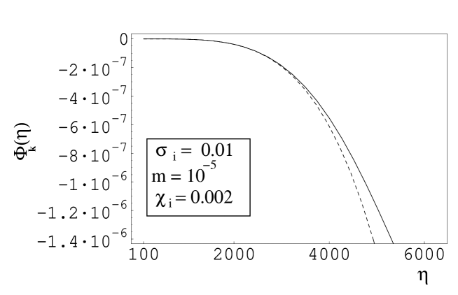
FIG. 1.: The full curve shows the result of a numerical integration for the case ${\cal H}_{\rm i}=0.01$, and for the set of parameters reported in the figure. The dashed curve shows the approximate analytical solution based on Eqs. (4.10) and (4.20).

In Figs. 1, 2 and 3 we report, as full curves, the results of the numerical integration for a quadratic potential. The analytical results of Eqs. (4.18)–(4.21), based on the slow-roll approximation, are also illustrated, for comparison, by the dashed curves.

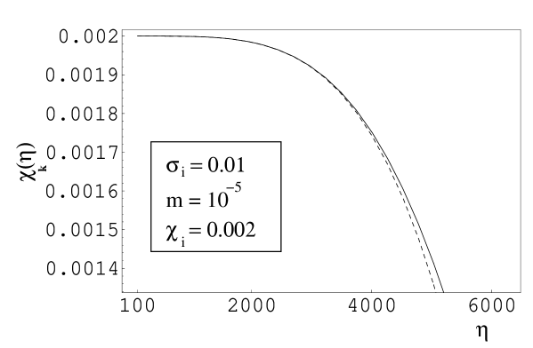
FIG. 2.: Evolution of $\chi_{k}$, reported for the same set of parameters as in Fig. 1. The dashed curve corresponds to the approximate analytical result of Eq. (4.19).

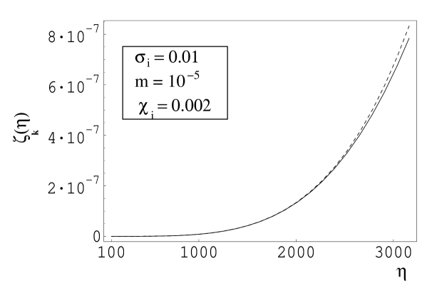
FIG. 3.: Evolution of $\zeta_{k}$, for the same set of parameters as in Figs. 1 and 2. The numerical result (full curve) is compared with the approximate analytical result of Eq. (4.21) (dashed curve).

B Radiation-dominated oscillations

During the radiation-dominated regime, and for a quadratic potential, the axion evolution equation (2.7) can be written as

$$\frac{d^{2}g}{d\tau^{2}}+\mu^{2}\tau^{2}g=0,~{}~{}~{}~{}~{}g=\sigma a,$$ (4.24)

and its exact solution can be given in terms of Bessel functions [40] as

$$g(\tau)=\sqrt{\tau}{\cal C}_{1/4}\bigg{(}\frac{\mu\tau^{2}}{2}\biggr{)},$$ (4.25)

where ${\cal C}_{1/4}$ is a linear combination (with constant coefficients) of Bessel functions of order $1/4$ and $\mu\tau^{2}/2\sim m(t-t_{\rm i})$. By imposing the correct boundary conditions and normalization, in such a way that $\sigma(\tau)\to\sigma_{\rm i}$ for $\tau\to 1$, we obtain

$$\sigma(\tau)=\frac{\sigma_{\rm i}}{\sqrt{\tau}}\frac{1}{J_{1/4}(\mu/2)}J_{1/4}\biggl{(}\frac{\mu}{2}\tau^{2}\biggr{)},~{}~{}~{}~{}\eta_{\rm i}<\eta<\eta_{\sigma},$$ (4.26)

where $J_{1/4}$ is the first-kind Bessel function. Notice that the small argument limit of this equation, for $\mu\ll 1$ and $\tau\rightarrow 1$, exactly gives the result (4.18), obtained in the slow-roll approximation. This exact analytical solution can also be used as a consistency check of the quadratic approximations when the potential, during slow-roll, has a more complicated analytical form.

The onset of the axion oscillations can be determined from the first zero of $J_{1/4}(\mu\tau^{2}/2)$, which occurs for

$$\frac{\mu\tau^{2}}{2}\simeq 2.78,$$ (4.27)

namely for

$$\tau_{\rm m}=\frac{\epsilon_{1}}{\sqrt{\mu}},~{}~{}~{}~{}~{}\epsilon_{1}\simeq 2.35.$$ (4.28)

Different definitions of the oscillation starting time, for instance related to the breakdown of the slow-roll approximation, would lead to similar numerical values, i.e. to Eq. (4.28) with $\epsilon_{1}\simeq(12)^{1/4}$. In the large argument limit ($\mu/2\tau^{2}\gg 1$) of Eq. (4.26) the solution finally describes the oscillating regime,

$$\sigma(\tau)\simeq\frac{2\sigma_{\rm i}}{\tau^{3/2}\sqrt{\pi\mu}J_{1/4}(\mu/2)}\cos{\biggl{(}\frac{\mu\tau^{2}}{2}-\frac{3}{8}\pi\biggr{)}},~{}~{}~{}~{}\eta_{\rm osc}<\eta<\eta_{\sigma},$$ (4.29)

where the phase and amplitude of oscillations are fixed by the initial conditions.

An approximate solution of Eq. (2.24), similar to Eq. (4.26), holds for the axion fluctuations, namely

$$\chi_{k}(\tau)\simeq\frac{\chi_{\rm i}(k)}{\sqrt{\tau}}\frac{1}{J_{1/4}(\mu/2)}J_{1/4}\biggl{(}\frac{\mu}{2}\tau^{2}\biggr{)},~{}~{}~{}~{}~{}~{}\eta_{\rm i}<\eta<\eta_{\sigma},$$ (4.30)

whose small and large argument limits lead, respectively, to

$$\chi_{k}(\tau)\simeq\chi_{\rm i}(k)\left[1-\frac{\mu^{2}}{20}\left(\tau^{4}-1\right)\right],$$ (4.31)

$$\chi_{k}(\tau)\simeq\frac{2\chi_{\rm i}(k)}{\tau^{3/2}\sqrt{\pi\mu}J_{1/4}(\mu/2)}\cos{\biggl{(}\frac{\mu\tau^{2}}{2}-\frac{3}{8}\pi\biggr{)}}.$$ (4.32)

We notice that Eq. (4.30) is obtained by solving the approximate evolution equation

$$\chi_{k}^{\prime\prime}+2{\cal H}\chi_{k}^{\prime}+m^{2}a^{2}\chi_{k}\simeq 0,$$ (4.33)

i.e. neglecting the terms containing the Bardeen potentials in Eq. (2.24). In the slow-roll approximation, as previously stressed, these terms can be neglected for a generic potential term. However, they can also be neglected in the oscillating phase, provided the potential is well approximated by a quadratic form. We have explicitly checked that the exact analytical solutions (4.26) and (4.30) are in perfect agreement with the results of a numerical integration performed with a quadratic potential.

Thus, for a potential which is generic during the slow-roll phase (but still quadratic during the oscillating regime) it will be sufficient to work out the slow-roll solutions specific to that potential, from Eqs. (4.4), (4.9), and match them (with their first derivative) to the WKB solutions of Eqs. (4.24) and (4.33), namely

$$\sigma(\tau)\simeq\frac{\sigma_{2}}{\sqrt{2a_{\rm i}^{2}\mu\tau^{3}}}\cos{\biggl{(}\frac{\mu\tau^{2}}{2}+\beta\biggr{)}},$$ (4.34)

$$\chi_{k}(\tau)\simeq\frac{\chi_{2}(k)}{\sqrt{2a_{\rm i}^{2}\mu\tau^{3}}}\cos{\biggl{(}\frac{\mu\tau^{2}}{2}+\gamma\biggr{)}}.$$ (4.35)

The matching will allow a determination of the precise amplitudes and phases of $\sigma$ (and $\chi_{k}$) in terms of $\sigma_{\rm i}$ (and $\chi_{\rm i}(k)$).

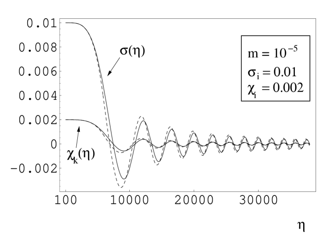
FIG. 4.: The exact, numerical evolution of $\sigma$ and $\chi_{k}$ (full curves) is compared with the interpolating solution (dashed curves) obtained by matching the slow-roll solutions (4.18) and (4.19) with the WKB approximated solutions (4.34) and (4.35), valid during the radiation-dominated oscillations of the axion.

As an application of this technique let us consider the example of the quadratic potential, using the slow-roll solutions for $\tau<\tau_{\rm m}$. The result of this exercise is reported in Fig. 4 where, with the full curves, we illustrate the numerical results (coinciding exactly with the analytical solutions). With the dashed curves we show the interpolating solutions obtained by matching Eqs. (4.18) and (4.19) (obtained in the slow-roll approximation) with the WKB solutions (4.34) and (4.35), valid in the oscillating regime.

The time evolution of $\sigma(\eta)$ and $\chi_{k}(\eta)$ explains why, for $\tau\geq\tau_{\rm m}$ (i.e. after the slow-roll regime where $\Phi_{k}\sim a^{4}$ according to Eq. (4.10)), the Bardeen potential enters a phase of linear evolution (in conformal time). This feature is illustrated in Fig. 5, where we report the numerical results for the evolution of the Bardeen potential, computed for different values of the axion mass.

An analytical estimate of the slope of the linear regression for $\Phi_{k}$, after the end of the radiation-dominated slow roll, can be obtained from the Hamiltonian constraint (2.20), which can be recast in the following form:

$$\frac{\partial}{\partial\tau}(\tau^{3}\Phi_{k})=-\frac{\tau^{4}}{12}\biggl{[}\frac{\partial\sigma}{\partial\tau}\frac{\partial\chi_{k}}{\partial\tau}+\mu^{2}\tau^{2}\sigma\chi_{k}\biggr{]},$$ (4.36)

where we only assumed a quadratic form for the axion potential. By using the WKB solutions (4.34) and (4.35) we obtain

$$\Phi_{k}=-\frac{\sigma_{2}\chi_{2}(k)}{96a_{\rm i}^{2}}~{}\mu\tau-\frac{\sigma_{2}\chi_{2}(k)}{384a_{\rm i}^{2}\mu\tau^{3}}\biggl{[}-12\cos{(2\gamma+\mu\tau^{2})}+18\int^{\mu\tau^{2}/2}\frac{dx}{x}\cos{(x+\gamma)}\biggr{]},$$ (4.37)

where the integral can be expressed in terms of ${\rm Ci}(w)=-\int_{w}^{\infty}\frac{\cos{x}}{x}dx$ and ${\rm Si}(w)=\int_{0}^{w}\frac{\sin{x}}{x}dx$, and we have assumed $\beta=\gamma$. The oscillating terms are suppressed by $\tau^{-3}$ and can be neglected (in agreement with the numerical results of Fig. 5), since we are considering the regime $\tau>\tau_{\rm m}\gg 1$. On top of the oscillating terms, the amplitude of the term responsible for the linear growth can be extracted from the numerical solutions by fitting their asymptotic behaviour with the line

$$\Phi_{k}(\eta)=\sigma_{\rm i}\chi_{\rm i}[-\epsilon_{2}-\epsilon_{3}\sqrt{\mu}\tau],~{}~{}~{}~{}~{}~{}\tau>\tau_{\rm m}.$$ (4.38)

In the case of a quadratic potential we obtain

$$\epsilon_{2}\simeq 0.001,~{}~{}~{}~{}~{}~{}~{}~{}~{}~{}~{}\epsilon_{3}\simeq 0.0437.$$ (4.39)

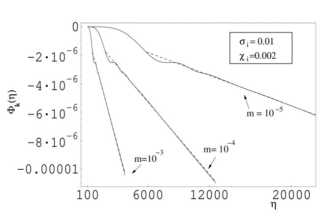
FIG. 5.: The results of the numerical integrations for the Bardeen potential are illustrated by the full curves for a quadratic potential and for different values of the mass. The dashed lines represent the linear fit of Eq. (4.38).

The accuracy of this result can be appreciated from Fig. 5, where the dashed lines (barely distinguishable from the numerical solutions) are plotted according to Eqs. (4.38), (4.39). A different form of the potential will not affect the angular coefficient of the regression (which is determined by the phase of the radiation-dominated oscillations), but only the constant $\epsilon_{2}$.

It may be interesting to look also at the analytical estimate of $\epsilon_{3}$, for a quadratic potential. The initial amplitudes $\sigma_{2}$ and $\chi_{2}(k)$ of Eq. (4.37) are determined by the large argument limit of the exact solutions, Eqs. (4.29) and (4.32). In this case we get

$$\epsilon_{3}^{\rm th}=\frac{\Gamma^{2}(5/4)}{6\pi}=0.0435,$$ (4.40)

in excellent agreement with (4.39). For a generic potential, we could also determine $\epsilon_{3}$ by adopting an approximate procedure, i.e. by taking the slow-roll solutions for $\chi_{k}$ and $\sigma$ from Eqs. (4.4) and (4.9), and matching them in $\tau_{\rm m}$ to the WKB solutions (4.34) and (4.35), in order to determine amplitude and phase.

The linear growth of the Bardeen potential continues until $\rho_{\sigma}$, decreasing as $a^{-3}$, equals $\rho_{\rm r}$. This happens at a time $\tau_{\sigma}$ such that

$$12{\cal H}^{2}\simeq a^{2}m^{2}\sigma^{2}.$$ (4.41)

The expansion of Eq. (4.29) for $\mu\ll 1$ then gives

$$\tau_{\sigma}=\frac{\epsilon_{4}}{\sigma_{\rm i}^{2}~{}\sqrt{\mu}},~{}~{}~{}~{}~{}~{}~{}~{}~{}~{}~{}~{}\epsilon_{4}=\frac{3\pi}{2\Gamma^{2}(5/4)}\simeq 5.74.$$ (4.42)

From Eq. (4.38) we can then finally obtain the value of the Bardeen potential, at the onset of the phase of $\sigma$-dominated oscillations. By using the value of $\tau_{\sigma}$ given by Eq. (4.42), the result is

$$\Phi_{k}(\eta_{\sigma})\simeq\epsilon_{5}\frac{\chi_{\rm i}(k)}{\sigma_{\rm i}},~{}~{}~{}~{}~{}\epsilon_{5}=\epsilon_{4}\epsilon_{3}\simeq 0.25.$$ (4.43)

C The axion-dominated oscillations

Using standard techniques suitable for the oscillating regime [38, 26], Eqs. (2.10) and (2.7) can be solved and, in the case of a quadratic potential, the oscillating terms lead to a geometry that reproduces (but only on the average) a matter-dominated Universe. The oscillating corrections will be suppressed for large (cosmic or conformal) times, and can be easily computed in the cosmic-time gauge, where:

$$\dot{H}=-\frac{1}{4}\dot{\sigma}^{2},$$ (4.44)

$$H^{2}=\frac{1}{12}\biggl{[}\dot{\sigma}^{2}+m^{2}\sigma^{2}\biggr{]},$$ (4.45)

$$\ddot{\sigma}+3H\dot{\sigma}+m^{2}\sigma=0.$$ (4.46)

Using the auxiliary variable $Z=d\sigma/d\ln{a}$, which satisfies

$$\frac{dZ}{d\sigma}=-3\bigg{(}1-\frac{Z^{2}}{12}\biggr{)}\biggl{(}1+4\frac{Z}{\sigma}\biggr{)},$$ (4.47)

and defining two angular variables $(r,\theta)$,

$$Z=\sqrt{12}\sin{\theta},~{}~{}~{}~{}\sigma=r\cos{\theta},$$ (4.48)

(such that $H=mr/\sqrt{12}$), the following two equations are obtained:

$$\dot{\theta}=-\frac{\sqrt{3}}{4}mr\sin{2\theta}-m,~{}~{}~{}~{}~{}~{}~{}~{}~{}~{}~{}\dot{r}=-\frac{\sqrt{3}}{2}mr^{2}\sin^{2}{\theta}.$$ (4.49)

They can be solved, and the solutions expanded for large times at any order in $1/t$.

A similar procedure can be carried out in conformal time. Equations (2.7)–(2.10) are equivalent to the following set of equations

$$r^{\prime}=-\frac{\sqrt{3}}{2}ma_{\rm f}\eta^{2}r^{2}\sin^{2}{\biggl{(}\frac{ma_{f}\eta^{3}}{3}\biggr{)}},~{}~{}~{}~{}~{}~{}~{}~{}~{}\sigma=r\cos{\biggl{(}\frac{ma_{f}\eta^{3}}{3}\biggr{)}}$$ (4.50)

(where $a_{f}$ is an appropriate dimensionful integration constant), and their solution leads to the expansion

$$a(\eta)\simeq a_{\rm f}\biggl{[}\eta^{2}-\frac{3}{2a_{\rm f}^{2}m^{2}\eta^{4}}\cos{\biggl{(}\frac{2~{}ma_{\rm f}\eta^{3}}{3}\biggr{)}}+{\cal O}(\frac{1}{\eta^{5}})\biggr{]},$$ (4.51)

$${\cal H}(\eta)\simeq\biggl{[}\frac{2}{\eta}+\frac{3}{ma_{\rm f}\eta^{4}}\sin{\biggl{(}\frac{2~{}ma_{\rm f}\eta^{3}}{3}\biggr{)}}+{\cal O}(\frac{1}{\eta^{5}})\biggr{]},$$ (4.52)

$$\sigma(\eta)\simeq\frac{4\sqrt{3}}{ma_{\rm f}\eta^{3}}\cos{\biggl{(}\frac{ma_{\rm f}\eta^{3}}{3}\biggr{)}}+{\cal O}(\frac{1}{\eta^{5}}).$$ (4.53)

A posteriori, as a cross-check, Eqs. (4.53) can be inserted into Eqs. (2.6)–(2.10), to see that all terms up to ${\cal O}(1/\eta^{5})$ cancel, as expected.

In the phase dominated by the oscillating axion the effective gravitational source is pressureless, on the average. By inserting the condition $\langle p_{\sigma}\rangle=0$ into the background and perturbation equations, we get

$$\langle\delta_{\sigma}(k)\rangle\sim-2\langle\Phi_{k}\rangle,~{}~{}~{}~{}~{}~{}~{}~{}~{}~{}~{}\langle\delta_{\rm r}(k)\rangle\sim-2\langle\delta_{\sigma}(k)\rangle,$$ (4.54)

which can be inserted into Eq. (2.39), obtaining

$$\langle\zeta_{k}\rangle\simeq\frac{5}{6}\langle\delta_{\sigma}(k)\rangle\simeq-\frac{5}{3}\langle\Phi_{k}\rangle.$$ (4.55)

when $\langle p_{\sigma}\rangle\sim 0$ and $\rho_{\sigma}\gg\rho_{\rm r}$.

Since $p_{\sigma}$ vanishes only on the average, more accurate solutions have to be supplemented by oscillating corrections. Using Eqs. (4.53) an approximate form of the perturbations in the oscillating regime can be obtained. One finds that $\delta_{\sigma}(k)$ and $\Phi_{k}$ are almost constant (up to oscillations), i.e.

$$\delta_{\sigma}(\eta)\simeq-\frac{1}{2}\Phi_{0}(k)\biggl{[}1-\cos{\biggl{(}\frac{2a_{\rm f}m\eta^{3}}{3}\biggr{)}}\biggr{]},$$ (4.56)

$$\Phi_{k}(\eta)\simeq\Phi_{0}(k)\biggl{[}1-\frac{1}{ma_{\rm f}\eta^{3}}\sin{\biggl{(}\frac{2}{3}ma_{\rm f}\eta^{3}\biggr{)}}-\frac{4}{(ma_{\rm f}\eta^{3})^{2}}\cos{\biggl{(}2\frac{ma_{f}\eta^{3}}{3}\biggr{)}}\biggr{]},$$ (4.57)

$$\chi_{k}(\eta)\simeq\chi_{0}(k)\biggl{[}\sin{\biggl{(}\frac{ma_{\rm f}\eta^{3}}{3}\biggr{)}}+\frac{3}{ma_{\rm f}\eta^{3}}\cos{\biggl{(}\frac{ma_{\rm f}\eta^{3}}{3}\biggr{)}}\biggr{]},$$ (4.58)

where

$$\Phi_{0}(k)=\langle\Phi_{k}(\eta)\rangle,~{}~{}~{}~{}~{}~{}~{}~{}~{}\eta_{\sigma}<\eta<\eta_{\rm d},$$ (4.59)

and

$$\chi_{0}(k)=-\frac{4}{\sqrt{3}}\Phi_{0}(k).$$ (4.60)

The above solutions satisfy the evolution equations of the fluctuations up to ${\cal O}(\eta^{-5})$.

D The axion decay and the subsequent radiation-dominated phase

When the decay rate of the axion equals the cosmological expansion rate, energy is transferred from the coherent oscillations of $\sigma$ to the radiation produced by the axion decay. The radiation produced thanks to the decay of the axion will quickly dominate the expansion and the second radiation-dominated phase will take place.

The Bardeen potential prior to decay is given by Eq. (4.57) while, after the decay, its evolution equation (2.29) reduces to

$$\Phi^{\prime\prime}+4{\cal H}\Phi^{\prime}+2({\cal H}^{2}+{\cal H}^{\prime})\Phi-\frac{1}{3}\nabla^{2}\Phi=0,~{}~{}~{}~{}~{}~{}\eta>\eta_{\rm d},$$ (4.61)

and the corresponding exact solution can be expressed as [26]

$$\Phi_{k}(\eta)=\frac{1}{\eta^{3}}\biggl{[}B_{1}(k)(\omega\eta\cos{\omega\eta}-\sin{\omega\eta})+B_{2}(k)(\omega\eta\sin{\omega\eta}+\cos{\omega\eta})\biggr{]},~{}~{}~{}\eta>\eta_{\rm d},$$ (4.62)

where $\omega=k/\sqrt{3}$. In the sudden approximation, the two (dimensional) arbitrary constants $B_{1}(k)$ and $B_{2}(k)$ can be uniquely fixed by matching, at the decay time $\eta_{\rm d}$, the solutions (4.57) and (4.62) together with their first derivatives. The terms containing $(k\eta_{\rm d})$ are small and negligible for modes that are outside the horizon at the time of the axion decay, i.e. for the ones relevant to the physics of the observed CMBR anisotropies. Furthermore, terms proportional to inverse powers of $m/H_{\rm d}\sim M_{\rm P}^{2}/m^{2}$ are also small and can be consistently neglected. Hence, up to subleading terms, the final value of the Bardeen potential can be written as

$$\Phi_{k}(\eta)=\Phi_{0}(k)\left[2\cos{\left(\frac{2\beta}{3}\right)}-3\right]\biggl{[}\frac{\cos{\omega\eta}}{(\omega\eta)^{2}}-\frac{\sin{\omega\eta}}{(\omega\eta)^{3}}\biggr{]},$$ (4.63)

where $\beta=m\eta_{\rm d}a(\eta_{\rm d})\sim m/H_{\rm d}\sim M_{\rm P}^{2}/m^{2}$. The $\beta$-dependent prefactor is a consequence of the approximation of sudden decay where the axion field is assumed to decay at a specific time $\eta_{\rm d}$. This sudden approximation also neglects the possible (exponential) damping of the oscillations in $\Phi_{k}$ arising in Eq. (4.57).

It will now be shown that the $\beta$-dependent prefactor is an artefact of the sudden approximation. In a realistic model of decay, in fact, the energy-momentum tensors of the radiation fluid and of the axion will not be separately conserved, because of their relative coupling induced by the friction term $\Gamma(\sigma^{\prime}/a)^{2}$, which leads, in cosmic time, to the generalized conservation equations:

$$\dot{\rho}_{\sigma}+(3H+\Gamma)(\rho_{\sigma}+p_{\sigma})=0,$$ (4.64)

$$\dot{\rho}_{\rm r}+4H\rho_{\rm r}-\Gamma(\rho_{\sigma}+p_{\sigma})=0.$$ (4.65)

The fluctuations $\chi_{k}$ will experience a similar damping,

$$\chi^{\prime\prime}+(2{\cal H}+\Gamma a)\chi^{\prime}-\nabla^{2}\chi+\frac{\partial^{2}V}{\partial\sigma^{2}}a^{2}\chi-4\sigma^{\prime}\Phi^{\prime}+2\frac{\partial V}{\partial\sigma}a^{2}\Phi=0,$$ (4.66)

while the $\Phi_{k}$ evolution will still be described by Eq. (2.29). This treatment of the damping of the fluctuations was suggested in [8] (see also [41]). The effect of $\Gamma$ is, primarily, to induce a damping in the oscillations of the background and of the axion fluctuations according to Eqs. (4.65) and (4.66). Moreover, the (damped) fluctuations of the axionic field will also influence the dynamics of $\Phi_{k}$ according to Eq. (2.29). The time-dependent oscillations of Eq. (4.57) (occurring in the absence of friction) will then be further suppressed if $\Gamma\neq 0$ (more details will be given in the following section). As a consequence, the $\beta$-dependent correction tends to disappear from Eq. (4.63), leading to the final result

$$\Phi_{k}(\eta)=3\Phi_{0}(k)\biggl{[}\frac{\sin{\omega\eta}}{(\omega\eta)^{3}}-\frac{\cos{\omega\eta}}{(\omega\eta)^{2}}\biggr{]}.$$ (4.67)

In the equation for $\Phi_{k}$ the effect of the finite duration $\Gamma^{-1}$ is then equivalent to averaging over the decay time. At the end of the following section, numerical examples of the decay will be discussed in detail.

V Background and perturbation equations for $\sigma_{\i}>1$

If $\sigma_{\rm i}>1$, the epoch of axion domination precedes the oscillation epoch. The previous solutions for the slow-roll regime are still valid, and the axion starts dominating when

$$\rho_{\rm r}a^{2}=6{\cal H}^{2}\simeq Va^{2},$$ (5.1)

i.e., for a quadratic potential, when

$$\tau=\tau_{\sigma}\simeq\frac{(12)^{1/4}}{\sqrt{\mu\sigma_{\rm i}}}.$$ (5.2)

If $\sigma_{\rm i}\simeq 1$, then

$$\tau_{\rm m}\simeq\tau_{\sigma},$$ (5.3)

the axion oscillates almost immediately after becoming dominant, and the amplitude of the Bardeen potential at the onset of the oscillatory phase is obtained from Eq. (4.20) as

$$\Phi_{k}(\eta_{\rm m})\simeq-\frac{\mu^{2}}{84}\chi_{\rm i}(k)\sigma_{\rm i}\tau_{\rm m}^{4}=-{1\over 7}{\chi_{\rm i}(k)\over\sigma_{\rm i}}\simeq-{1\over 7}\chi_{\rm i}(k).$$ (5.4)

If the initial value $\sigma_{\rm i}$ is larger than $1$, but not too large, then Eqs. (5.3) and (4.20) are still valid, but Eq. (5.4) is to be multiplied by the factor $\sigma_{\rm i}^{2}$, arising from a short period of axion dominance toward the end of the slow-roll evolution (see below). This effect, for moderate values of $\sigma_{\rm i}$, is illustrated in Fig 6 where, for the given parameters of the plot, the final amplitude of the Bardeen potential is estimated as

$$\Phi_{k}(\eta_{\rm m})\simeq-\epsilon_{6}\chi_{\rm i}(k)\sigma_{\rm i},~{}~{}~{}~{}~{}~{}~{}~{}~{}~{}~{}\epsilon_{6}=0.143$$ (5.5)

still in good agreement with the approximate value $1/7$ of Eq. (5.4).

FIG. 6.: The full curves are the results of numerical integrations for the case $\sigma_{\rm i}>1$. The dashed curves correspond to the approximated results of Eqs. (4.20) and (5.5).

If $\sigma_{\rm i}\gg 1$, then $\tau_{\rm m}\gg\tau_{\sigma}$, and a phase of inflationary expansion dominated by the axion potential will take place between $\tau_{\sigma}$ and $\tau_{\rm m}$. During this phase the axion slowly rolls, the radiation energy-density is quickly diluted as $\rho_{\rm r}\sim a^{-4}$, and the time evolution of the fluctuations is correspondingly modified. The Hamiltonian and momentum constraints (2.20) and (2.21) can now be combined to give

$$4\nabla^{2}\Phi_{k}=3{\cal H}\sigma^{\prime}\chi_{k}-\Phi_{k}{\sigma^{\prime}}^{2}+\sigma^{\prime}\chi_{k}^{\prime}+V_{,\sigma}a^{2}\chi_{k},$$ (5.6)

and the speed of sound of Eq. (2.33) becomes

$$c_{s}^{2}\simeq 1+\frac{2a^{2}}{3{\cal H}\sigma^{\prime}}V_{,\sigma},$$ (5.7)

from which, using Eq. (2.40),

$$\delta p_{\rm nad}=\frac{2V_{\sigma}}{3{\cal H}\sigma^{\prime}}\biggl{[}\Phi_{k}{\sigma^{\prime}}^{2}+\sigma^{\prime}\chi_{k}^{\prime}-3{\cal H}\sigma^{\prime}\chi_{k}-a^{2}V_{,\sigma}\chi_{k}\biggr{]}.$$ (5.8)

The combination of Eqs. (5.6) and (5.8) leads to

$$\delta p_{\rm nad}=\frac{8V_{,\sigma}}{3{\cal H}\sigma^{\prime}}\nabla^{2}\Phi_{k}.$$ (5.9)

Hence, from Eq. (2.35), we get that $\zeta_{k}^{\prime}\sim 0$ at large scales.

According to its definition, on the other hand, the constancy of $\zeta_{k}$ implies, in cosmic time, that

$$\Phi_{k}\biggl{(}\frac{2+\alpha_{1}}{1+\alpha_{1}}\biggr{)}+\frac{\dot{\Phi}_{k}}{H}\frac{1}{1+\alpha_{1}}$$ (5.10)

is also a constant, where

$$\alpha_{1}=-{\dot{H}}/{H^{2}}.$$ (5.11)

It follows that, during inflation, we can parametrize the evolution of $\Phi_{k}$, to lowest order, as

$$\Phi_{k}=A\biggl{(}{\dot{H}}/{H^{2}}\biggr{)},$$ (5.12)

where $A$ is a constant controlled by the value of the Bardeen potential at the beginning of inflation. Assuming a quadratic potential for $\tau<\tau_{\sigma}$ we have, from Eq. (5.4), $A\simeq-(1/7)(\chi_{\rm i}(k)/\sigma_{\rm i})(H^{2}/\dot{H})_{\tau_{\sigma}}$. By using the dynamics of slow-roll inflation,

$$H^{2}\simeq\frac{m^{2}}{12}\sigma^{2},$$ (5.13)

$$\dot{\sigma}\simeq-\frac{m^{2}}{3H}\sigma,$$ (5.14)

we can deduce that

$$\frac{\dot{H}}{H^{2}}\simeq-\frac{4}{\sigma^{2}}.$$ (5.15)

Using Eq. (5.15) we finally obtain the Bardeen potential at the onset of the phase of $\sigma$-dominated oscillations:

$$\Phi_{k}(\tau_{\rm m})\sim\sigma_{\rm i}\chi_{\rm i}(k),$$ (5.16)

where we used the expression for $A$ given above and the fact that $\sigma(\tau_{\sigma})=\sigma_{\rm i}$ and $\sigma(\tau_{\rm m})\sim{\cal O}(1)$. For $\tau>\tau_{\rm m}$ the axion eventually oscillates, and the subsequent evolution has the same features as already discussed in the previous section, for the case $\sigma_{\rm i}<1$.

In the following, the dynamics of the decay will be investigated numerically, and Eq. (2.29) will be solved together with Eqs. (4.65) and (4.66). In order to illustrate the results let us recall that, in the absence of friction ($\Gamma=0$ in Eqs. (4.66)), the evolution of $\chi_{k}$ and $\Phi_{k}$, during the axion-dominated oscillations, is given by Eqs. (4.57) and (4.58). In particular,

$$\Phi_{k}(\eta)\simeq\Phi_{0}(k)+\delta\Phi_{k}(\eta),$$ (5.17)

where $\delta\Phi_{k}(\eta)$ is an oscillating function decaying as $\eta^{-3}\sim t^{-1}$. The frequency of oscillation of $\delta\Phi_{k}$ is controlled by the axion mass. In analogy with Eq. (5.17) we can also define $\delta\chi_{k}$ which, for $\Gamma=0$, corresponds to the oscillating function appearing in Eq. (4.58). The evolution of $t\delta\Phi_{k}$ and of $\delta\chi_{k}$, for $\Gamma=0$, is represented by the full bold curves of Figs. 7 and 8. Notice that $\delta\Phi_{k}$ and $\delta\chi_{k}$ oscillate very fast and that, for our illustrative purpose, we have plotted their amplitudes calculated as the average of the semi-difference between the maximum and the minimum of each oscillation, and the semi-difference between the successive maximum and the same minimum.

If the oscillations of $\delta\Phi_{k}$ are only suppressed by a power-law function of time, we have seen that there are mass-dependent terms that appear in the amplitude of the Bardeen potential after the decay. The integration of Eqs. (2.29) and of (4.65) and (4.66) shows however that, with the inclusion of the appropriate friction terms (due to the decay) into the energy-momentum conservation equations, the oscillations in $\delta\Phi_{k}$ and $\delta\chi_{k}$ are exponentially suppressed and, in such a case, no mass-dependent correction is left in the amplitude of the Bardeen potential (the asymptotic, constant value of $\Phi_{k}$ is however unaffected by such a damping mechanism). The damping of the oscillations, on a time scale of order $\Gamma^{-1}$, is illustrated by the dashed curves of Figs. 7 and 8.

FIG. 7.: Time evolution of the amplitude of the $\delta\Phi_{k}$ oscillations (multiplied by $t$ in cosmic time), with and without the damping term due to the axion decay.

If we compare the sudden-decay approximation, discussed in the previous section, with the numerical results of Figs. 7 and 8, we see that the finite duration of the decay process can be physically represented as a dynamical average to zero of the oscillatory terms in the evolution of $\Phi_{k}$. In view of these results, when matching $\Phi_{k}$ to the post-decay phase, we should take into account the fact that all the derivatives of $\Phi_{k}$ are exponentially suppressed with respect to $\Phi_{k}/t_{\rm d}$, and thus can be safely neglected. This leads to the result reported in Eq. (4.67).

FIG. 8.: Time evolution of the amplitude of the $\delta\chi_{k}$ oscillations, with and without the damping term due to the axion decay.

VI Large-scale adiabatic fluctuations

In order to discuss the direct impact of our results on the possible generation of the observed CMBR anisotropies, the evolution of the large-scale metric fluctuations should be followed down to the matter-dominated phase, for all times $\eta>\eta_{\rm eq}$. In particular, the phase and the amplitude of the Bardeen potential prior to $\eta_{\rm eq}$ will fix the initial conditions for the subsequent evolution of the inhomogeneities, and will be crucial to determine whether they are of adiabatic or isocurvature nature.

We recall that, after the axion decay, the amplitude of the Bardeen potential has been computed as

$$\Phi_{k}(\eta)=3\Phi_{0}(k)\biggl{[}\frac{\sin{\omega\eta}}{(\omega\eta)^{3}}-\frac{\cos{\omega\eta}}{(\omega\eta)^{2}}\biggr{]},~{}~{}~{}~{}~{}\eta\leq\eta_{\rm eq},$$ (6.1)

where, as in the previous section, $\omega=k/\sqrt{3}$. For $\eta>\eta_{\rm eq}$, matter domination sets in, the background satisfies $2{\cal H}^{\prime}+{\cal H}^{2}=0$, so that the evolution of the Bardeen potential (outside the horizon) is described by

$$\Phi_{k}^{\prime\prime}+3{\cal H}\Phi_{k}^{\prime}=0,~{}~{}~{}~{}~{}{\cal H}=\frac{2}{\eta},$$ (6.2)

whose solution can be written as

$$\Phi_{k}(\eta)=A(k)+\frac{B(k)}{\eta^{5}},~{}~{}~{}~{}\eta\geq\eta_{\rm eq}.$$ (6.3)

Imposing the continuity of the solutions (6.1) and (6.3) and of their first derivatives at $\eta=\eta_{\rm eq}$ one obtains:

$$A(k)=\frac{3\Phi_{0}(k)}{5x_{\rm eq}^{3}}[-2x_{\rm eq}\cos{x_{\rm eq}}+(x_{\rm eq}^{2}+2)\sin{x_{\rm eq}}],$$ (6.4)

$$B(k)=\frac{3\Phi_{0}(k)\eta_{\rm eq}^{5}}{5x_{\rm eq}^{3}}[3x_{\rm eq}\cos{x_{\rm eq}}+(x_{\rm eq}^{2}-3)\sin{x_{\rm eq}}],$$ (6.5)

where $x_{\rm eq}=\omega\eta_{\rm eq}\equiv k\eta_{\rm eq}/\sqrt{3}$. For scales that are outside the horizon prior to decoupling, $x_{\rm eq}\ll 1$, and Eq. (6.3) becomes

$$\Phi_{k}(\eta)=\Phi_{0}(k)\biggl{[}1+\frac{(k\eta_{\rm eq})^{2}}{75}\biggl{(}\frac{\eta_{\rm eq}}{\eta}\biggr{)}^{5}\biggr{]},~{}~{}~{}~{}~{}~{}~{}\eta>\eta_{\rm eq}.$$ (6.6)

For $\eta>\eta_{\rm eq}$ the decaying mode is highly suppressed, and we are then in the situation of constant Bardeen potential right after equality, with an amplitude $\Phi_{0}(k)$, which (recalling the previous results (4.43), (5.4), (5.16)) is completely determined by the axion spectrum and by the initial conditions of the axion background. More precisely, the final amplitude can be parametrized as follows

$$\Phi_{0}(k)\equiv\Phi_{k}(\eta_{\rm d})\equiv-f(\sigma_{\rm i})\chi_{\rm i}(k),$$ (6.7)

where

$$f(\sigma_{\rm i})=c_{1}\sigma_{\rm i}+\frac{c_{2}}{\sigma_{\rm i}}-c_{3},$$ (6.8)

and

$$c_{1}\simeq 0.13,~{}~{}~{}~{}~{}~{}~{}c_{2}\simeq 0.25,~{}~{}~{}~{}~{}~{}~{}c_{3}\simeq 0.01.$$ (6.9)

The above coefficients $c_{i}$ have been obtained by integrating numerically the evolution equations of the background and of the fluctuations for different values of $\sigma_{\rm i}$ (both larger and smaller than $1$). Then, following the hint of the analytical results obtained by solving the evolution piece-wise, the final value of $\Phi_{k}(\eta)$ has been fitted with Eq. (6.8), and the values reported in Eq. (6.9) have been determined.

The value (6.8) of the Bardeen potential provides the initial condition for the subsequent hydrodynamical evolution. Such evolution will allow us to determine, in turn, the precise value of the temperature fluctuations through the Sachs–Wolfe effect. In particular, the modes that are outside the horizon for $\eta_{\rm eq}<\eta<\eta_{\rm dec}$ will determine the large-scale temperature fluctuations relevant to the COBE observations.

By perturbing the corresponding conservation equations on a matter-dominated background, we obtain:

$$\delta_{\rm r}^{\prime}-\frac{4}{3}\nabla^{2}v_{\rm r}-4\Phi^{\prime}=0,$$ (6.10)

$$v_{\rm r}^{\prime}-\frac{1}{4}\delta_{\rm r}-\Phi=0,$$ (6.11)

$$\delta_{\rm m}^{\prime}-\nabla^{2}v_{\rm m}-3\Phi^{\prime}=0,$$ (6.12)

$$v_{\rm m}^{\prime}+{\cal H}v_{\rm m}-\Phi=0,$$ (6.13)

where $\delta_{\rm m}=\delta\rho_{\rm m}/\rho_{\rm m}$ and $v_{\rm m}$, following the notation of the previous sections, are the gauge-invariant density contrast and velocity potential of the matter fluctuations. Also, in the above equations,

$${\cal H}=\frac{2}{\eta},~{}~{}~{}~{}~{}\rho_{\rm m}a^{2}=\frac{24}{\eta^{2}}.$$ (6.14)

As already stressed at the beginning of this section, $\Phi$ is constant during the matter-dominated phase. Using this property we can now work out the specific relations between the different fluid variables, for modes that are outside the horizon right after equality, so as to explicitly check the adiabaticity of the fluid perturbations.

The system of Eqs. (6.10)–(6.13) can be easily solved by going to Fourier space. For $v_{\rm m}$ we have

$$kv_{\rm m}(k)\simeq\frac{k\eta}{3}\Phi_{0}(k),~{}~{}~{}~{}~{}~{}~{}k\eta\ll 1.$$ (6.15)

Since $\vec{\nabla}v_{\rm m}$ (evaluated outside the horizon) contributes directly to the Sachs–Wolfe effect, it is important to notice that this term is subleading with respect to the other contributions arising in the case of adiabatic fluctuations. We will indeed show that, unlike $\vec{\nabla}v_{\rm m}$, which is suppressed, the contrast $\delta_{\rm r}$ is instead constant outside the horizon, and proportional to $\Phi_{0}(k)$.

Inserting $v_{\rm r}$ from Eq. (6.10) into Eq. (6.11) we get a decoupled equation for $\delta_{\rm r}$, namely,

$$\delta_{\rm r}^{\prime\prime}+\frac{k^{2}}{3}\delta_{\rm r}=-\frac{4}{3}k^{2}\Phi_{0}(k).$$ (6.16)

The general solution is

$$\delta_{\rm r}(k\eta)=A_{1}\cos{\omega\eta}+B_{1}\sin{\omega\eta}+4\Phi_{0}(k)[\cos{\omega\eta}-1],$$ (6.17)

and the constants $A_{1}$ and $B_{1}$ can be determined by consistency with the other equations and with the Hamiltonian constraint (2.20) written in the case of a matter-radiation fluid. The final result is:

$$\delta_{\rm r}(k,\eta)=\frac{4}{3}\Phi_{0}(k)\biggl{[}\cos{\omega\eta}-3\biggr{]}$$ (6.18)

$$kv_{\rm r}(k,\eta)=\frac{\Phi_{0}(k)}{\sqrt{3}}\sin{\omega\eta},$$ (6.19)

$$\delta_{\rm m}(k,\eta)=-2\Phi_{0}(k)-\frac{\Phi_{0}(k)}{6}(k\eta)^{2},$$ (6.20)

$$kv_{\rm m}(k,\eta)=\frac{(k\eta)}{3}\Phi_{0}(k).$$ (6.21)

Notice that, outside the horizon, $kv_{\rm m}\equiv kv_{\rm r}$ as required by local thermodynamical equilibrium. Furthermore, for $k\eta\ll 1$, the velocities of the two fluids are proportional to $(k\eta)$. When the modes are outside the horizon, Eqs. (6.18) and (6.20) imply that the density contrasts $\delta_{\rm r}$ and $\delta_{\rm m}$ are both constant and proportional according to

$$\delta_{\rm r}\simeq(4/3)\delta_{\rm m}.$$ (6.22)

This result has a simple physical interpretation, and implies the adiabaticity of the fluid perturbations. The entropy per matter particle is indeed proportional to $S=T^{3}/n_{\rm m}$, where $n_{\rm m}$ is the number density of matter particles and $T$ is the radiation temperature. The associated entropy fluctuation, $\delta S$, satisfies

$$\frac{\delta S}{S}=\frac{3}{4}\delta_{\rm r}-\delta_{\rm m},$$ (6.23)

where we used the fact that $\rho_{\rm r}\sim T^{4}$ and that $\rho_{\rm m}=mn_{\rm m}$, where $m$ is the typical mass of the particles in the matter fluid. Equation (6.22) thus implies $\delta S/S=0$, in agreement with the adiabaticity of the fluctuations.

A Sachs-Wolfe effect and COBE scales

The fluctuations of the Bardeen potential and of the radiation density contrast are sources of a slight temperature difference between photons coming from different sky directions. This is the essence of the Sachs–Wolfe effect [42]. In terms of the gauge-invariant variables introduced in the present analysis, the various contributions to the Sachs–Wolfe effect, along the $\vec{n}$ direction, can be written as [26, 29]

$$\frac{\Delta T}{T}(\vec{n},\eta_{0},x_{0})=\biggl{[}\frac{\delta_{\rm r}}{4}+\vec{n}\cdot\vec{\nabla}v_{\rm b}+\Phi\biggr{]}(\eta_{\rm dec},\vec{x}(\eta_{\rm dec}))-\int_{\eta_{0}}^{\eta_{\rm dec}}(\Phi^{\prime}+\Psi^{\prime})(\eta,\vec{x}(\eta))d\eta,$$ (6.24)

where $\eta_{0}$ is the present time, and $\vec{x}(\eta)=\vec{x}_{0}-\vec{n}(\eta-\eta_{0})$ is the unperturbed photon position at the time $\eta$ for an observer in $\vec{x}_{0}$. The term $\vec{v}_{\rm b}$ is the peculiar velocity of the baryonic matter component. We are preliminarily interested in the effects of scales still outside the horizon at the time of the matter-radiation equality, which are the scales relevant to the observations of the COBE-DMR experiment [14, 43]. In order to correctly take into account the constraints imposed by the COBE normalization on the spectral amplitude of the Bardeen potential, let us compare the relative weight of the different terms appearing in the Sachs-Wolfe formula (6.24).

From Eq. (6.19) we can see that, for our adiabatic initial conditions, the fluctuation in the matter velocity potential is subleading for superhorizon scales, suppressed by the term $k\eta\ll 1$ with respect to the constant values of $\delta_{\rm r}$ and $\Phi_{k}$. Furthermore, since $\Phi^{\prime}\simeq 0$ and $\Psi=\Phi$, the integrated Sachs–Wolfe effect can also be neglected. By inserting Eq. (6.18) into Eq. (6.24) we thus obtain the usual result for adiabatic fluctuations, namely

$$\frac{\Delta T}{T}(\vec{n},\eta_{0},x_{0})=\frac{1}{3}\Phi(\eta_{\rm dec},\vec{x}(\eta_{\rm dec})),$$ (6.25)

to be used for the comparison of our theoretical predictions with the COBE normalization.

On the other hand, by taking the Legendre transform at the present time $\eta_{0}$, the temperature fluctuations of Eq. (6.24) can be generally expanded into spherical harmonic functions, $Y_{\ell m}$, as

$$\frac{\Delta T}{T}(\vec{x}_{0},\vec{n},\eta_{0})=\sum_{\ell,m}a_{\ell m}(\vec{x}_{0})Y_{\ell m}(\vec{n}),$$ (6.26)

where the coefficients $a_{\ell m}$ define the angular power spectrum $C_{\ell}$ by

$$\biggl{\langle}a_{\ell m}\cdot a_{\ell^{\prime}m^{\prime}}^{*}\biggr{\rangle}=\delta_{\ell\ell^{\prime}}\delta_{mm^{\prime}}C_{\ell},$$ (6.27)

and determine the two-point correlation function of the temperature fluctuations, namely

$$\left\langle{\delta T\over T}(\vec{n}){\delta T\over T}(\vec{n}^{\prime})\right\rangle_{{~{}}_{\!\!(\vec{n}\cdot\vec{n}^{\prime}=\cos\vartheta)}} = \sum_{\ell\ell^{\prime}mm^{\prime}}\biggl{\langle}a_{\ell m}a_{\ell^{\prime}m^{\prime}}^{*}\biggr{\rangle}Y_{\ell m}(\vec{n})Y_{\ell^{\prime}m^{\prime}}^{*}(\vec{n^{\prime}})$$ (6.28)

$$= {1\over 4\pi}\sum_{\ell}(2\ell+1)C_{\ell}P_{\ell}(\cos\vartheta).$$ (6.29)

These coefficients $C_{\ell}$, in turn, are related through Eq. (6.25), to the power spectrum of $\Phi_{0}(k)$, and for $2\leq\ell\ll 100$ they can be expressed as [44]

$$C_{\ell}\simeq\frac{2}{9\pi}\int_{0}^{\infty}\frac{dk}{k}\biggl{\langle}|\Phi_{0}(k)|^{2}\biggr{\rangle}k^{3}j_{\ell}^{2}[k(\eta_{0}-\eta_{\rm dec})].$$ (6.30)

As already stressed, the spectrum of the Bardeen potential is fully determined, in our context, by the initial spectrum of axionic fluctuations amplified by the pre-big bang dynamics. A self-contained derivation of such a spectrum, including the mass contribution, is presented in Appendix A. Consider first the case of minimal pre-big bang models, whose related spectrum is reported in Eq. (A.14). The spectrum of curvature perturbations will then be, at large scales,

$$k^{3}\left|\Phi_{0}(k)\right|^{2}=f^{2}(\sigma_{\rm i})k^{3}\left|\chi_{k}\right|^{2}=f^{2}(\sigma_{\rm i})\biggl{(}\frac{H_{1}}{M_{\rm P}}\biggr{)}^{2}\left(k\over k_{1}\right)^{n-1},~{}~{}~{}~{}~{}~{}k<k_{1},$$ (6.31)

where $k_{1}$ is the maximal amplified comoving frequency, i.e., in our conventions, the frequency at which only one axion per cell of phase-space is produced. From $k_{1}$, a typical curvature scale $H_{1}$ (which can be, at most, of the order of the string mass) can be obtained:

$$H_{1}=\frac{k_{1}}{a_{1}}\leq M_{\rm s}.$$ (6.32)

The particular value of the scale $H_{1}$ may be regarded as a phenomenological parameter of the chosen model of pre-big bang evolution. Even assuming, according to the standard lore [45], that $M_{\rm s}\sim 10^{-1}~{}M_{\rm P}$, still the exact relation of $H_{1}$ to $M_{\rm s}$ depends on the detailed dynamics of a highly curved and strongly coupled background. The approach of the present investigation has been to include all the theoretical indetermination into $H_{1}$, trying to have a reasonable control of all the other numerical factors associated with the post-big bang evolution. In Eq. (6.31) the particular value of $n$ depends upon the specific model of pre-big bang evolution [15, 21]. In the case of a ten-dimensional model with an isotropic six-dimensional internal space, the line element can be written as

$$ds^{2}=dt^{2}-a^{2}(t)\gamma_{ij}dx^{i}dx^{j}-b^{2}(t)\gamma_{ab}dy^{a}dy^{b},$$ (6.33)

where $i,j$ run over the three external space-like dimensions and $a,b$ run over the six internal dimensions. Defining as

$$r=\frac{\dot{V}_{6}V_{3}}{2V_{6}\dot{V}_{3}}$$ (6.34)

the relative rate of variation of the external $V_{3}=a^{3}$ and internal $V_{6}=b^{6}$ volumes, the spectral index $n$ can be expressed as [21]

$$n=\frac{4+6r^{2}-2\sqrt{3+6r^{2}}}{1+3r^{2}}.$$ (6.35)

The case of flat spectrum (i.e. $n=1$) corresponds to the case $r=\pm 1$. If internal dimensions are static (i.e. $r=0$), then $n=4-2\sqrt{3}\simeq 0.53$. Blue spectra are allowed when the rate of variation of the external volume is much smaller than the internal one. The maximal $n$ achievable in this case is $n=2$, corresponding to the case of static external manifold ($r\to\infty$).

Bearing in mind Eqs. (6.32) and (6.35), we can use Eq. (6.31) and perform the integral of Eq. (6.30). For $-3<n<3$ the integral appearing in Eq. (6.30) can be done analytically [44] and the result is

$$C_{\ell}^{(SW)}=\frac{2^{n}}{72}~{}f^{2}(\sigma_{\rm i})\biggl{(}\frac{H_{1}}{M_{P}}\biggr{)}^{2}\biggl{(}\frac{\omega_{0}}{\omega_{1}}\biggr{)}^{n-1}\frac{\Gamma(3-n)\Gamma(\ell-\frac{1}{2}+\frac{n}{2})}{\Gamma^{2}(2-\frac{n}{2})\Gamma(\ell+\frac{5}{2}-\frac{n}{2})}.$$ (6.36)

Here $\omega_{0}\simeq 10^{-18}$ Hz and $\omega_{1}(t_{0})=H_{1}a_{1}/a_{0}$ are, respectively, the proper frequencies corresponding to the present horizon scale and to the present value of the cut-off scale $k_{1}$:

$$\omega_{1}(t_{0})=(H_{1}~{}H_{\rm eq})^{1/2}\biggl{(}\frac{\Gamma}{m}\biggr{)}^{1/6}\sigma_{\rm i}^{-2/3}z_{\rm eq}^{-1},~{}~{}~{}~{}~{}~{}~{}~{}~{}~{}~{}\sigma_{\rm i}<1,$$ (6.37)

$$\omega_{1}(t_{0})=(H_{1}~{}H_{\rm eq})^{1/2}\biggl{(}\frac{\Gamma}{m}\biggr{)}^{1/6}\sigma_{\rm i}^{1/2}Z_{\sigma}^{-1}z_{\rm eq}^{-1},~{}~{}~{}~{}~{}~{}\sigma_{\rm i}>1.$$ (6.38)

(we have rescaled $\omega_{1}$ taking into account the kinematics of the various cosmological phases from $t_{1}$ down to $t_{0}$). The factor $Z_{\sigma}=(a_{\rm osc}/a_{\sigma})$ denotes the amplification of the scale factor during the phase of axion-dominated, slow-roll inflation, for the case $\sigma_{\rm i}>1$. Notice that $\omega_{1}(t_{0})$ depends on the mass, on the initial amplitude of the axion background and on the axion decay rate. If the axion decays at a typical scale fixed by Eq. (3.4), Eqs. (6.37) and (6.38) lead to

$$\omega_{1}(t_{0}) \simeq 10^{29}\omega_{0}\left(H_{1}\over M_{\rm P}\right)^{1/2}\left(m\over\sigma_{\rm i}^{2}M_{\rm P}\right)^{1/3},~{}~{}~{}~{}~{}~{}~{}~{}~{}~{}~{}~{}~{}~{}~{}~{}~{}~{}~{}\sigma_{\rm i}<1,$$ (6.39)

$$\simeq 10^{29}\omega_{0}\left(\sigma_{\rm i}H_{1}\over M_{\rm P}\right)^{1/2}\left(m\over\ M_{\rm P}\right)^{1/3}Z_{\sigma}^{-1},~{}~{}~{}~{}~{}~{}~{}~{}~{}~{}~{}~{}~{}~{}\sigma_{\rm i}>1$$ (6.40)

(we have used $H_{0}\simeq 10^{-6}H_{\rm eq}\simeq 10^{-60}M_{\rm P}$). Hence, in spite of the fact that the initial axionic spectrum does not have any mass dependence, the mass appears again when computing the amplitude of the spectrum at the present horizon scale $\omega_{0}$.

The amplitude of the Bardeen potential, on the other hand, is constrained by the COBE normalization of the quadrupole coefficient $C_{2}$, which in our case is given by

$$C_{2}=\alpha^{2}_{n}f^{2}(\sigma_{\rm i})\left(H_{1}\over M_{\rm P}\right)^{2}\left(\omega_{0}\over\omega_{1}\right)^{n-1},$$ (6.41)

where

$$\alpha_{n}^{2}=\frac{2^{n}}{72}{\Gamma(3-n)\Gamma\left({3+n\over 2}\right)\over\Gamma^{2}\left({4-n\over 2}\right)\Gamma\left({9-n\over 2}\right)}.$$ (6.42)

Using the experimental result [46]

$$C_{2}=(1.9\pm 0.23)\times 10^{-10},$$ (6.43)

we are thus led to the bounds

$$\alpha^{2}_{n}f^{2}(\sigma_{\rm i})\sigma_{\rm i}^{2(n-1)/3}\left(H_{1}\over M_{\rm P}\right)^{(5-n)/2}\left(m\over M_{\rm P}\right)^{-(n-1)/3}10^{-29(n-1)}\simeq 1.9\times 10^{-10},~{}~{}~{}~{}\sigma_{\rm i}<1,$$ (6.44)

$$\alpha^{2}_{n}f^{2}(\sigma_{\rm i})Z_{\sigma}^{n-1}\sigma_{\rm i}^{(1-n)/2}\left(H_{1}\over M_{\rm P}\right)^{(5-n)/2}\left(m\over M_{\rm P}\right)^{-(n-1)/3}10^{-29(n-1)}\simeq 1.9\times 10^{-10},\,~{}~{}\sigma_{\rm i}>1.$$ (6.45)

These constraints, imposed by the COBE normalization, will be discussed at the end of the present section, and combined with other theoretical constraints pertaining to the various models of background evolution.

B Acoustic peak region

In the previous discussion of the modes that are outside the horizon before decoupling, we have completely neglected the possible scattering of radiation with baryons. In fact, if we move to smaller angular scales (i.e. typically to $\ell~{}\raise 1.72218pt\hbox{$>$}\kern-6.99997pt\lower 2.6694pt\hbox{$\sim$}~{}100$), the main contribution to the CMBR temperature fluctuations comes from the oscillations of the various plasma quantities, the so-called Sakharov oscillations [47]. A correct approach to this problem is then to perturb consistently the Boltzmann equations for the different species of the plasma [48, 49, 50]. Furthermore it can be relevant to discuss the case of a smooth transition between radiation and matter dominated epochs. In such a context it becomes difficult to provide an analytical description of the system and, in order to compute the patterns of the acoustic oscillations, we will indeed present some numerical examples in the third part of the present section.

It is however useful to emphasize that the phases of the Bardeen potential for the adiabatic mode of Eq. (6.1) determine not only the relative weight of the Sachs–Wolfe contributions, but also the specific phase of the oscillatory patterns at small scales in the temperature fluctuations. For scales $\ell~{}\raise 1.72218pt\hbox{$>$}\kern-6.99997pt\lower 2.6694pt\hbox{$\sim$}~{}100$ the contribution to the temperature perturbations given in Eq. (6.24) is dominated by acoustic oscillations. This aspect can be appreciated by looking at Eqs. (6.18)–(6.21) in the limit $k\eta>1$, where the peculiar velocity of baryonic matter does not oscillate. Instead, from Eq. (6.18), we find that the terms $\delta_{\rm r}/4$ and $\Phi$, appearing in Eq. (6.24), combine to give a single term oscillating like a cosine:

$$\frac{\Delta T}{T}(k,\eta_{0},\eta_{\rm dec})\simeq\frac{1}{4}\delta_{\rm r}(k,\eta_{\rm dec})+\Phi_{0}(k)\sim\frac{\Phi_{0}(k)}{3}\cos{\omega\eta_{\rm dec}}.$$ (6.46)

In this argument the interactions of baryons with the radiation fluid have been neglected. The dynamics of $(\Delta T/T)_{k}$ can be obtained from an exact Boltzmann equation with source term provided by Compton scattering coupled to the continuity and Euler equations for the fluid variables. Before recombination, Compton scattering is very rapid and therefore the Boltzmann, Euler and continuity equations for the photon–baryon system can be expanded in powers of the Compton scattering time [49, 50]. Within this approximation the baryon velocity field is damped and $(\Delta T/T)_{k}$ oscillates as a cosine for adiabatic initial conditions. In the approximation of [49, 50], the oscillations in $(\Delta T/T)_{k}$ have an amplitude proportional to $(1+R)^{-1/4}$ where $R(\eta)=3\rho_{\rm b}/(4\rho_{\rm r})$. This result simply tells that the baryonic content of the plasma determines the height of the first peak. Notice that this is in sharp contrast with what happens in the case of light axions [17, 18], where the Bardeen potential is quadratic in the axion fluctuations, and the initial conditions for the hydrodynamical evolution are of the isocurvature type. This implies, in particular, that the oscillatory patterns of the CMBR anisotropies will be shifted by $\pi/2$ if compared with the case discussed in the present paper.

C Constraints on pre-big bang models

In this subsection we will discuss the bounds imposed by the COBE normalization, together with other constraints following from the evolution of the background geometry. Let us start with the axion spectrum of minimal pre-big bang models, Eq. (6.31). In such a case, and for a flat Harrison–Zeldovich spectrum (i.e. $n=1$), the COBE normalization is inconsistent with a cut-off $H_{1}$ at the standard value $M_{\rm s}\sim 10^{-1}~{}M_{\rm P}$ of the string mass scale [45]. By using $n=1$, and taking for $\sigma_{\rm i}$ the value minimizing $f(\sigma_{\rm i})$,

$$\sigma_{\rm i}^{\rm min}=\sqrt{\frac{c_{2}}{c_{1}}}\simeq 1.38,~{}~{}~{}~{}~{}~{}~{}~{}f(\sigma_{\rm i}^{\min})\simeq 0.34,$$ (6.47)

we have indeed, from Eqs. (6.41)–(6.43),

$$H_{1}\simeq 5.2\times 10^{-4}~{}M_{\rm P}.$$ (6.48)

However, the precise value of $H_{1}$ is one of the main uncertainties of pre-big bang models. As we shall see in a moment, the value $H_{1}=M_{\rm s}$ (or $H_{1}=M_{\rm GUT}$) may become consistent with the COBE normalization for non-flat (blue) spectra, and even for a strictly flat spectrum in the case of non-minimal implementations of the pre-big bang scenarios.

Let us first recall the various constraints to be imposed on the spectrum. The condition (6.44) is to be combined with the constraint (3.7), the condition (6.45) with the constraint (3.12), which are required for the consistency of the corresponding classes of background evolution. Both conditions are to be intersected with the experimentally allowed range of the spectral index. We will use (as a reference value) the generous upper bound [1], $n~{}\raise 1.72218pt\hbox{$<$}\kern-8.00003pt\lower 2.6694pt\hbox{$\sim$}~{}1.4$. Also, for our illustrative purpose, we will take the maximally extended range of allowed values of the axion mass, satisfying the nucleosynthesis constraint $m~{}\raise 1.72218pt\hbox{$>$}\kern-6.99997pt\lower 2.6694pt\hbox{$\sim$}~{}10$ TeV.

We will assume, finally, that in the case $\sigma_{\rm i}>1$ the axion-driven inflation is short enough, to avoid a possible contribution to $C_{\ell}$ arising from the metric fluctuations directly amplified from the vacuum during such a phase of axionic inflation. This requires that the smallest amplified frequency mode $\omega_{\sigma}$, crossing the horizon at the beginning of inflation, at decoupling be still larger than the Hubble horizon at the corresponding epoch. This imposes the condition $\omega_{\sigma}(t_{0})=H_{\sigma}(a_{\sigma}/a_{0})>\omega_{\rm dec}(t_{0})=H_{\rm dec}(a_{\rm dec}/a_{0})$ , namely

$$Z_{\sigma}~{}\raise 1.72218pt\hbox{$<$}\kern-8.00003pt\lower 2.6694pt\hbox{$\sim$}~{}10^{27}\sigma_{\rm i}\left(m\over M_{\rm P}\right)^{5/6},$$ (6.49)

to be added to the constraint (3.12) for $\sigma_{\rm i}>1$.

The allowed region in the plane $\{\log\sigma_{\rm i},\log(m/M_{\rm P})\}$ is illustrated in Fig. 9 for $H_{1}=10^{-2}M_{\rm P}$, using for the inflation factor the parametrization $Z_{\sigma}=\exp((\sigma_{\rm i}^{2}-1)/8)$. Along the thin full curves the parameters satisfy the COBE normalization, for fixed values of $n$, ranging from $1.1$ to $1.4$ (the condition (6.49), in this case, is always automatically satisfied). A growing (“blue”) spectrum is thus allowed even if $H_{1}\sim M_{\rm s}$, for a wide range of axion masses, and for a (narrower) range of values of $\sigma_{\rm i}$. In particular, for the case $H_{1}=10^{-2}M_{\rm P}$, we find $1~{}\raise 1.72218pt\hbox{$>$}\kern-6.99997pt\lower 2.6694pt\hbox{$\sim$}~{}\sigma_{\rm i}~{}\raise 1.72218pt\hbox{$>$}\kern-6.99997pt\lower 2.6694pt\hbox{$\sim$}~{}10^{-4}$, for $\sigma_{\rm i}<1$. For $\sigma_{\rm i}>1$ the results are complementary for the spectral index, but there are much more stringent bounds on $\sigma_{\rm i}$, because the inflationary red-shift factor $Z_{\sigma}$ grows exponentially with $\sigma_{\rm i}^{2}$. As a consequence, the allowed region for $\sigma_{\rm i}>1$ is distorted and compressed, as illustrated in Fig. 9.

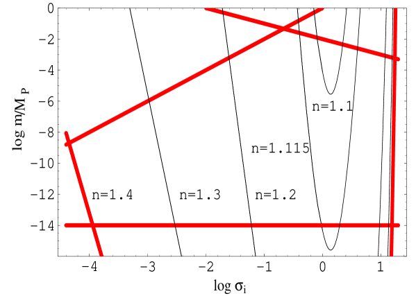
FIG. 9.: Allowed values of $\sigma_{\rm i}$ and $m$ (in Planck units) according to Eqs. (6.44), (6.45), with $H_{1}=10^{-2}M_{\rm P}$. The allowed region (within the thick lines) is bounded by the condition $n<1.4$ (left and right bold lines), by the nuclesosynthesis constraint $m>10$ TeV (lower bold line), by the condition (3.7) (upper left bold line) and (3.12) (upper right bold line).

The allowed region may be further extended if the inflation scale $H_{1}$ is lowered (see for instance [51]), and a flat ($n=1$) or almost flat spectrum may become possible if $c_{2}\alpha_{1}H_{1}~{}\raise 1.72218pt\hbox{$<$}\kern-8.00003pt\lower 2.6694pt\hbox{$\sim$}~{}10^{-5}M_{\rm P}\sigma_{\rm i}$, for $\sigma_{\rm i}<1$, and if $c_{1}\alpha_{1}H_{1}~{}\raise 1.72218pt\hbox{$<$}\kern-8.00003pt\lower 2.6694pt\hbox{$\sim$}~{}10^{-5}M_{\rm P}/\sigma_{\rm i}$, for $\sigma_{\rm i}>1$ (see Eqs. (6.44), (6.45)). The corresponding allowed values of $H_{1}$ and $\sigma_{\rm i}$ are illustrated in Fig. 10 for $m=10^{-9}M_{\rm P}$, and for three different values of $n$ around $1$.

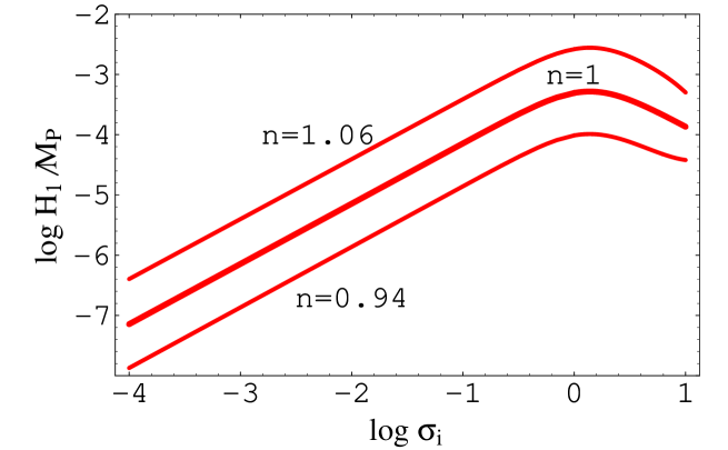
FIG. 10.: Allowed values of $H_{1}$ as a function of $\sigma_{\rm i}$ for different values of the spectral index and for $m=10^{-9}M_{\rm P}$.

However, a flat spectrum may be allowed even keeping pre-big bang inflation at the string scale ($H_{1}\sim M_{\rm s}$), provided we consider a non-minimal pre-big bang scenario. In that context, in fact, the high-frequency branch of the axionic spectrum may be modified, getting steeper enough to match the string-scale normalization at the end-point of the spectrum, while the low-frequency branch remains flat (or quasi-flat, see Appendix), to agree with large-scale observations. Examples of realistic pre-big bang backgrounds producing such an axion spectrum have been presented already in [19].

A non-minimal spectrum can be parametrized by the Bogoliubov coefficients (which will be given in Eq. (A.17)), in terms of a generic break-scale $k_{s}$ and of the high-frequency slope parameter $\delta$. In that case, for a long and/or steep enough high-frequency branch of the spectrum, the large-scale amplitude may be suppressed sufficiently to allow flat (or even red) spectra at the COBE scale. In fact, for the non-minimal spectrum (A.17), the normalization condition (6.41) becomes

$$C_{2}=\alpha^{2}_{n}f^{2}(\sigma_{\rm i})\left(H_{1}\over M_{\rm P}\right)^{2}\left(\omega_{0}\over\omega_{1}\right)^{n-1}\left(\omega_{s}\over\omega_{1}\right)^{\delta}.$$ (6.50)

Flat or red spectra ($n\leq 1$) are thus possible even for $H_{1}~{}\raise 1.72218pt\hbox{$>$}\kern-6.99997pt\lower 2.6694pt\hbox{$\sim$}~{}10^{-2}M_{\rm P}$, provided

$$\alpha^{2}_{1}f^{2}(\sigma_{\rm i})\left(\omega_{s}\over\omega_{1}\right)^{\delta}~{}\raise 1.72218pt\hbox{$<$}\kern-8.00003pt\lower 2.6694pt\hbox{$\sim$}~{}10^{-6}.$$ (6.51)

In order to illustrate this possibility we will choose a specific model of background by identifying $k_{s}$ with the equilibrium scale $k_{\rm eq}$, in such a way that $n$ corresponds to the spectral index of all scales relevant to the CMBR anisotropies, while $n+\delta$ provides the average spectral index for all other scales, up to $k_{1}$. We will also assume for the axion background the “natural” initial value $\sigma_{\rm i}=1$, so that

$$\frac{\omega_{1}}{\omega_{s}}=\frac{\omega_{1}}{\omega_{\rm eq}}\simeq 10^{27}\biggl{(}\frac{H_{1}}{M_{\rm P}}\biggr{)}^{1/2}\biggl{(}\frac{m}{M_{\rm P}}\biggr{)}^{1/3}.$$ (6.52)

The COBE normalization can then be written explicitly as

$$C_{2}=\alpha_{n}^{2}f^{2}(1)\biggl{(}\frac{H_{1}}{M_{P}}\biggr{)}^{(5-n-\delta)/2}\biggl{(}\frac{m}{M_{P}}\biggr{)}^{-(n-1+\delta)/3}10^{-[27\delta+29(n-1)]}.$$ (6.53)

By using the experimental value of $C_{2}$ given in Eq. (6.43) we can now obtain a relation between the high-frequency slope parameter $\delta$ and the spectral index $n$ at the COBE scale, for any given value of $H_{1}$ and $m$. In Fig. 11 we illustrate such a relation for different (realistic) values of $H_{1}$, and for a typical axion mass $m=10^{-9}M_{\rm P}$. It should be stressed that, for $n\simeq 1$, and $\sigma_{\rm i}$ of order 1 (i.e. near the minimum of $f(\sigma_{\rm i})$), the curves at constant $H_{1}$ are almost insensitive to the values of $m$, and remain stable even if we change $m$ by various orders of magnitude, as illustrated in Fig. 12.

We have also reported, in Fig. 11, the (present) most stringent bounds on $n$, obtained by a recent analysis of the CMBR anisotropies and large-scale structures [55, 56], i.e. $0.87\leq n\leq 1.06$. They are all compatible with $H_{1}\simeq M_{\rm s}$, provided we allow for a small break of the minimal spectrum, with $\delta\simeq 0.2$–$0.3$. On the other hand, as already stressed, no break at all is needed (i.e. $\delta=0$) if, for some dynamical mechanism (see for instance [51]) the string mass is lowered down to the GUT scale, i.e. $H_{1}\simeq 10^{-3}M_{\rm P}$.

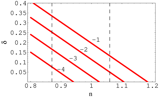
FIG. 11.: Relation between $\delta$ and $n$ for different values of $H_{1}$ (in Planck units), for $m=10^{-9}M_{\rm P}$, and for $\sigma_{\rm i}=1$. The vertical dashed lines denote the experimentally allowed range $0.87\leq n\leq 1.06$.

In Fig. 12 we have plotted the same curves of Fig. 11 for two, very different values of the axion mass, $10^{-9}M_{\rm P}$ (bold curves) and $10^{-14}M_{\rm P}$ (thin dashed curves). As clearly illustrated by the figure, the dependence on the mass is very mild, and it becomes practically inappreciable (for the given range of parameters) when $H_{1}$ approaches $M_{\rm GUT}$.

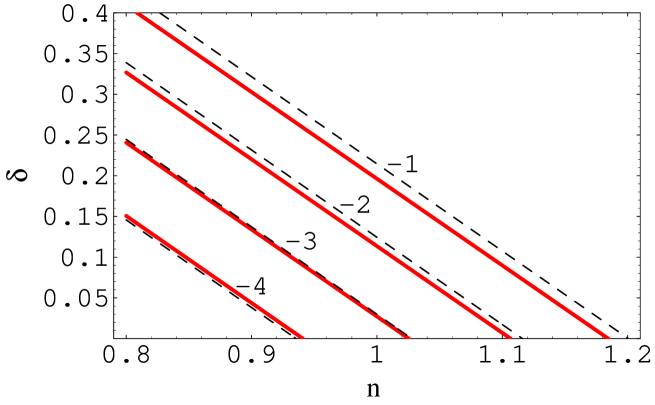
FIG. 12.: Stability of the curves of Fig. 10 for two different choices of the axion mass, $10^{-9}M_{\rm P}$ (bold curves) and $10^{-14}M_{\rm P}$ (thin dashed curves).

Having discussed the constraints imposed by the COBE normalization we can present now the plots of the angular coefficients $C_{\ell}$ for the scalar spectrum, in the case of a spatially flat background and for few relevant choices of the spectral index. In Figs. 13 and 14 the (scalar) angular power spectrum defined in Eq. (6.27) is reported for a flat, slightly red and slightly blue spectrum. In order to obtain the results of Figs. 13 and 14 we used the latest release of CMBFAST, relaxing the strict COBE normalization at $\ell=10$, in favour of a better general agreement of the overall fit.

In Figs. 13 and 14 we used the following values of the cosmological parameters, selected according to fits of CMBR anisotropy experiments [56]: $h_{0}=0.65$, $\Omega_{\Lambda}=0.7$, and $h_{0}^{2}\Omega_{b}=0.02$. The selected value of $h_{0}^{2}\Omega_{b}$ is rather robust, even if no final consensus has been reached on the second significant figure beyond $0.02$. We have also assumed the simplest scenario for the late-time cosmological evolution, with no significant effects of reionization.

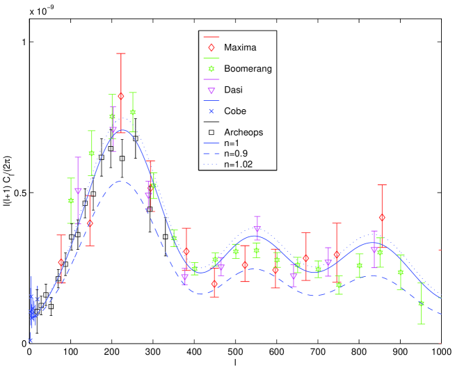
FIG. 13.: The spectrum of $C_{\ell}$ is illustrated for a fiducial set of parameters ($h_{0}=0.65$, $\Omega_{\rm b}=0.04733$, $\Omega_{\Lambda}=0.7$, $\Omega_{\rm m}=0.25267$) and for flat (full line, $n=1$), slightly red (dashed line, $n=0.9$) and slightly blue (dotted line, $n=1.02$) spectral indices.

In Fig. 13 the $C_{\ell}$ are plotted on a linear scale, whereas in Fig. 14 we present the same plot with a semi-logarithmic scale, in such a way that the region relevant to the COBE observations is less compressed. We recall, finally, that the flat, red and blue spectral indices may correspond to particular combinations of the parameters $H_{1},m,\delta$ and $\sigma_{\rm i}$, chosen in such a way as to satisfy the COBE normalization, Eq. (6.50).

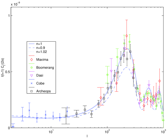
FIG. 14.: The same plot as in Fig. 13, but on a semi-logarithmic scale.

The data points reported in Figs. 13 and 14 are those from COBE [1, 2], BOOMERANG [4], DASI [5], MAXIMA [6] and ARCHEOPS [7]. Notice that the data reported in [7] fill the “gap” between the last COBE points and the points of [4, 5, 6]. Therefore, one could think of normalizing the spectra not to COBE but directly to ARCHEOPS. In spite of this possibility, the forthcoming MAP data will give even more accurate determination of the $C_{\ell}$ spectra. It will then be interesting to use these data in order to make more consistent and accurate determinations of the pre-big bang parameter space.

VII Concluding remarks

In the present paper the possible conversion of isocurvature, primordial axionic fluctuations into adiabatic, large-scale metric perturbations has been discussed in the context of the pre-big bang scenario. Depending upon the specific relaxation of the axionic background toward the minimum of the potential, a constant (and large enough) mode in the Bardeen potential can be generated, for scales that are still outside the horizon right after matter-radiation equality.

After analysing the dynamics of the background and of its fluctuations, the final amplitude and spectrum of the Bardeen potential has been related to the initial axion spectrum directly arising from the vacuum fluctuations amplified during the pre-big bang epoch. Our goal has been to include, with reasonable accuracy, the details of the post-big bang evolution, in such a way that the pre-big bang parameters could be directly constrained by the COBE normalization, and by the analysis of the Doppler-peak structure. All the theoretical uncertainty reflects in our lack of knowledge of $H_{1}$ which determines the end point of the primordal axion spectrum.

The main conclusion of this work is that a phenomenologically appealing spectrum of adiabatic scalar perturbations can naturally emerge from the simplest pre-big bang scenario through a conversion of the initial isocurvature perturbations of the Kalb-Ramond axion. Since, at the large scales tested by CMBR experiments, the above conversion preserves the scale-dependence of the original spectrum, it is important for the latter to be quasi-scale-invariant at large scales. This can be achieved, for instance, if the very early stages of pre-big bang cosmology at weak coupling involve a symmetric evolution of all $9$ spatial dimensions (modulo $T$-duality). Since the constant mode of the curvature fluctuations leads to adiabatic initial conditions for the fluid evolution after matter-radiation equality, the location of the Doppler peak is correctly reproduced.

On the other hand, the absolute normalization of fluctuations at large scales (say those relevant for COBE) depend on several details of the model. Indeed, the axion spectrum is naturally normalized at its end-point, given by our parameter $H_{1}$. If one takes, naively, $H_{1}\sim M_{\rm s}\sim 10^{17}~{}{\rm GeV}$ and assumes a flat spectrum one finds values of $\Delta T/T$ that are a couple of orders of magnitude too large when compared with COBE’s data. However, one can think of many (individual or combined) effects that can bring down our normalization to agree with the data, e.g.

• A slight (blue) tilt to the spectrum;

• A blue spectrum just at high frequency (i.e. for scales that exit late, during the strongly coupled regime);

• A lower $H_{1}/M_{\rm s}$ ratio;

• A lower $M_{\rm s}/M_{\rm P}$ ratio.

In the near future we hope to extend the present discussion to forthcoming CMBR anisotropy data at even smaller angular scales. It would be interesting to see if a combined analysis of the experimental data may give further useful hints on the parameter space of the scenario explored in the present investigation.

A Axionic spectra

During the pre-big bang phase the quantum mechanical fluctuations of the axionic field will be amplified from the initial vacuum state. The obtained spectrum provides the initial condition for the evolution of the axion fluctuations in the post-big bang phase. At very large-scales, such a spectrum will not depend so much upon the details of the pre-big bang evolution. At smaller scales, however, it can be strongly affected by specific dynamics of the strong coupling and high-curvature regime. In spite of the fact that the spectral slope at large scales is not affected by high energy corrections, the large scale amplitude is affected and, in particular, a steeper slope at small scales has important consequences for the normalization of the low-frequency branch of the spectrum. In this appendix we will consider, separately, the axion spectrum obtained in the case of minimal and non-minimal pre-big bang models.

1 Minimal pre-big bang models

The linearized evolution of massive axion inhomogeneities $\chi_{k}$, neglecting their coupling to scalar metric perturbations, in a spatially flat cosmological background, is described in general by the equation

$$\psi_{k}^{\prime\prime}+\biggl{[}k^{2}+m^{2}a^{2}-\frac{z^{\prime\prime}}{z}\biggr{]}\psi_{k}=0,$$ (A.1)

where

$$z=a~{}e^{\varphi/2},~{}~{}~{}~{}\psi_{k}=z\chi_{k}.$$ (A.2)

In the pre-big bang phase ($\eta<\eta_{1}$) the axion is massless. In the post-big bang, radiation-dominated phase, taking place for $\eta>\eta_{1}$, the gauge coupling freezes ($\varphi=$ const) and the axion acquires a mass. The produced axion spectrum, in principle, has a relativistic and a non-relativistic branch: this is because, in the radiation era, the proper momentum is red-shifted with respect to the rest mass, and the whole spectrum, mode by mode, tends to become non-relativistic. The spectral slope of the relativistic and non-relativistic branches of the spectrum are in general different. However, if the axion modes, as in the present case, become non-relativistic when they are still outside the horizon, the solution is then exactly the same as in the relativistic limit.

Consider first the relativistic branch of the spectrum. For $\eta<\eta_{1}$ the solution of Eq. (A.1) can be expressed in terms of the second-kind Hankel functions [40] as:

$$\psi_{k}(\eta)=\eta^{1/2}H_{\mu}^{(2)}(k\eta),$$ (A.3)

where $\mu$ depends on the parameters controlling the kinematics of the pre-big bang background (a specific example will be given below, see Eqs. (A.7) and (6.35)). In the radiation era, $\eta>\eta_{1}$, one has $z^{\prime\prime}/z=0$, and the evolution equation of $\psi_{k}$ acquires a massive correction:

$$\psi_{k}^{\prime\prime}+\left(k^{2}+m^{2}a^{2}\right)\psi_{k}=0,$$ (A.4)

Assuming that the axion mass is negligible at the transition epoch $\eta_{1}$, the solution (A.3) can be matched to the plane-wave solution

$$\psi_{k}={1\over\sqrt{k}}\left[c_{+}(k)e^{-ik\eta}+c_{-}(k)e^{ik\eta}\right],$$ (A.5)

and the final result for $\chi_{k}$ is

$$\chi_{k}(\eta)={c(k)\over a\sqrt{k}}\sin(k\eta),$$ (A.6)

where

$$c(k)\simeq\biggl{(}\frac{k}{k_{1}}\biggr{)}^{\frac{n-5}{2}},$$ (A.7)

with $n=4-2|\mu|$ . Note that the expression of the Bogoliubov coefficient $c(k)$ and of the mean number of produced axions, $\overline{n}_{k}=|c(k)|^{2}$, contains different numerical factors of order $1$. At the same time the maximal amplified momentum $k_{1}$ can be defined in different ways, all equivalent up to numerical factors. In the present analysis we will define the maximal scale $k_{1}$ as the energy scale where one axion is produced per unit volume of phase-space.

Consider now the non–relativistic spectrum in the case when the mode becomes non–relativistic while it is still outside the horizon. Defining as $k_{m}$ the limiting comoving frequency of a mode that becomes non-relativistic ($k_{m}=ma_{m}$) at the time it re-enters the horizon ($k_{m}=H_{m}a_{m}$), we find, in the radiation era [18, 19],

$$k_{m}=k_{1}\left(m\over H_{1}\right)^{1/2}.$$ (A.8)

We are thus considering modes with $k\ll k_{m}$. In order to estimate the spectrum, in this limit, let us write Eq. (A.4) in a form suitable for comparison with known results of parabolic cylinder equations:

$${d^{2}\psi_{k}\over dx^{2}}+\left({x^{2}\over 4}-b\right)\psi_{k}=0,~{}~{}~{}~{}~{}x=\eta(2\alpha)^{1/2},~{}~{}~{}~{}-b=k^{2}/2\alpha,$$ (A.9)

where

$$m^{2}a^{2}=\alpha^{2}\eta^{2},~{}~{}~{}~{}~{}~{}~{}~{}~{}~{}~{}~{}~{}~{}~{}~{}\alpha=mH_{1}a_{1}^{2},$$ (A.10)

and where $a\sim\eta$ has been assumed. The corresponding general solution can be written as

$$\psi=Ay_{1}(b,x)+By_{2}(b,x)~{},$$ (A.11)

where $y_{1}$ and $y_{2}$ are the even and odd parts of the parabolic cylinder functions [40]. The normalization to Eq. (A.6) in the relativistic limit (i.e. $x\to 0$) gives $A=0$ and

$$\psi_{k}\simeq c(k)\left(k\over 2\alpha\right)^{1/2}y_{2}(b,x).$$ (A.12)

Outside the horizon, $k\eta\ll 1$, and for non-relativistic modes, $k\ll ma$, we take (respectively) the limits $-bx^{2}\ll 1$ and $-b\ll x^{2}$, the solution can be expanded as $y_{2}\sim x\sim\eta\sqrt{2\alpha}$, so that the mass disappears from the amplitude:

$$|\chi_{k}|\simeq{|c(k)|k^{1/2}\over a_{1}\eta_{1}}.$$ (A.13)

The insertion of the spectrum (A.7), using $k_{1}=a_{1}H_{1}$, leads to the final result

$$k^{3/2}|\chi_{k}|\simeq H_{1}\biggl{(}\frac{k}{k_{1}}\biggr{)}^{\frac{n-1}{2}}.$$ (A.14)

2 Non-minimal pre-big bang evolution and spectral breaks

Equation (A.14) holds in the case of minimal pre-big bang models, where the dynamical evolution of the dilaton field is dictated by the solution of the low-energy equations of motion. However, when the dilaton enters the strong coupling regime, different types of scenarios may emerge. In particular, relation (A.2) defining the form of the axion pump field, may change in the infinite bare string-coupling limit, as suggested by the arguments recently developed in [51]. In the framework of [51] the axion coupling function, as well as the other coupling functions pertaining to fields of different spin, may have a finite limit for infinite bare string coupling. Hence, toward the end of the pre-big bang phase (i.e. when strong coupling is presumably reached),

$$z\sim a[c_{z}+{\cal O}(e^{-\varphi/2})],$$ (A.15)

where $c_{z}$ is a constant. Since the axionic pump field now depends only on the scale factor, it will naturally be steeper for small length scales. A complementary possibility, discussed in [19], is the presence of an intermediate high-energy phase, which precedes the standard radiation era, and which is still part of the accelerated pre-big bang regime, but in which the kinematics of the (usual) canonical pump field is significantly different from its low-energy behaviour.

In all these cases the obtained spectra, at small scales, are possibly steeper than in the case of minimal pre-big bang models. In the simplest case the spectrum will have only one break, at a momentum scale that will be conventionally denoted by $k_{s}$, and the Bogoliubov coefficients can be written in the form

$$|c_{k}|^{2} = \left(k\over k_{1}\right)^{n-5+\delta},~{}~{}~{}~{}~{}~{}~{}~{}~{}~{}~{}~{}~{}~{}~{}~{}~{}~{}~{}~{}~{}~{}k_{s}<k<k_{1},$$ (A.16)

$$= \left(k_{s}\over k_{1}\right)^{n-5+\delta}\left(k\over k_{s}\right)^{n-5},~{}~{}~{}~{}~{}~{}~{}~{}~{}~{}~{}~{}~{}~{}k<k_{s}.$$ (A.17)

Here $\delta>0$ parametrizes the slope of the break at high frequency, while $n$ is the usual spectral index appearing at large scales and computed on the basis of the perturbative evolution of the dilaton field. From Eq. (A.17) it can be argued that the steeper and/or the longer the high-frequency branch of the spectrum, the larger the suppression at low-frequency scales.

REFERENCES

- [1] C. L. Bennet et al., Astrophys. J. Lett. 464, L1 (1996).
- [2] M. Tegmark, Astrophys. J. Lett. 464, L35 (1996).
- [3] E. Gawiser and J. Silk, Phys. Rept. 333, 245 (2000).
- [4] C. B. Netterfield et al., Astrophys. J. 571, 604 (2002).
- [5] N. W. Halverson et al., Astrophys. J. 568, 38 (2002).
- [6] A. T. Lee et al., Astrophys. J. 561, L1 (2001).
- [7] A. Benoît et al., astro-ph/0210305.
- [8] V. Bozza, M. Gasperini, M. Giovannini and G. Veneziano, Phys. Lett. B543, 14 (2002).
- [9] G. Veneziano, Phys. Lett. B265, 287 (1991); M. Gasperini and G. Veneziano, Astropart. Phys. 1, 317 (1993).
- [10] J. E. Lidsey, D. Wands and E. J. Copeland, Phys. Rep. 337, 343 (2000).
- [11] M. Gasperini and G. Veneziano, Phys. Rep. 373, 1 (2003).
- [12] M. Gasperini and G. Veneziano, Phys. Rev. D50, 2519 (1994).
- [13] R. Brustein, M. Gasperini, M. Giovannini, V. Mukhanov and G. Veneziano, Phys. Rev. D51, 6744 (1995).
- [14] G. F. Smoot et al., Astrophys. J. 396, L1 (1992).
- [15] E. J. Copeland, R. Easther and D. Wands, Phys. Rev. D56, 874(1997).
- [16] E. J. Copeland, J. E. Lidsey and D. Wands, Nucl. Phys. B506, 407 (1997).
- [17] R. Durrer, M. Gasperini, M. Sakellariadou, and G. Veneziano, Phys. Lett. B436, 66 (1998).
- [18] R. Durrer, M. Gasperini, M. Sakellariadou, and G. Veneziano, Phys. Rev. D59, 43511 (1999).
- [19] M. Gasperini and G. Veneziano, Phys. Rev. D59, 43503 (1999).
- [20] M. Giovannini, Phys. Rev. D 59, 063503 (1999).
- [21] A. Melchiorri, F. Vernizzi, R. Durrer, and G. Veneziano, Phys. Rev. Lett. 83, 4464 (1999); F. Vernizzi, A. Melchiorri and R. Durrer, Phys. Rev. D63, 063501 (2001).
- [22] K. Enqvist and M. S. Sloth, Nucl. Phys. B626, 395 (2002).
- [23] D. H. Lyth and D. Wands, Phys. Lett. B524, 5 (2002).
- [24] T. Moroi and T. Takahashi, Phys. Lett. B522, 215 (2001) and Phys. Rev. D66, 063501 (2002).
- [25] H. Kodama and M. Sasaki, Prog. Theor. Phys. Suppl. 78, 1 (1984).
- [26] V.F. Mukhanov, H.A. Feldman, and R. H. Brandenberger, Phys. Rep. 215, 203 (1992).
- [27] S. Mollerach, Phys. Rev. D42, 313 (1990).
- [28] J. M. Bardeen, Phys. Rev. D22, 1882 (1980).
- [29] R. Durrer, Fund. of Cosmic Physics 15, 209 (1994).
- [30] D. H. Lyth, Phys. Rev. D31, 1792 (1984).
- [31] A. Liddle and D. Lyth, Phys. Rep. 231, 1 (1993).
- [32] K. Kim, Phys. Rev. Lett. 43, 103 (1979); M. Dine, W. Fischler and M. Srednicki, Phys. Lett. B104, 199 (1981).
- [33] J. Preskill, M. Wise and F. Wilczek, Phys. Lett. B120, 127 (1983).
- [34] P. Di Vecchia and G. Veneziano, Nucl. Phys. B171, 253 (1980).
- [35] J. Ellis, D. V. Nanopoulos and M. Quiros, Phys. Lett. B174, 176 (1986).
- [36] J. Ellis, C. Tsamish and M. Voloshin, Phys. Lett. B194, 291 (1987).
- [37] M. Gasperini, Phys. Lett. B327, 214 (1994).
- [38] M. S. Turner, Phys. Rev. D28, 1243 (1983).
- [39] D. Lyth, C. Ungarelli and D. Wands, astro-ph/0208055.
- [40] M. Abramowitz and I. A. Stegun, Handbook of mathematical functions (Dover, New York, 1972).
- [41] K. A. Malik, D. Wands, and C. Ungarelli, astro-ph/0211602.
- [42] R. K. Sachs and A. M. Wolfe, Astrophys. J. 147, 73 (1967).
- [43] G. Hinshaw et al., Astrophys. J. 464, L17 (1996).
- [44] R. Durrer, J. Phys. Stud. 5, 177 (2001).
- [45] V. Kaplunovsky, Phys. Rev. Lett. 55, 1036 (1985).
- [46] A. J. Banday et al., Astrophys. J. 475, 393 (1997).
- [47] A. D. Sakharov, Sov. Phys. JETP 22, 241 (1965).
- [48] H. Kodama and M. Sasaki, Int. J. Mod. Phys. A1, 265 (1986).
- [49] W. Hu and N. Sugiyama, Astrophys. J. 444, 489 (1995).
- [50] W. Hu and N. Sugiyama, Astrophys. J. 471, 542 (1996).
- [51] G. Veneziano, JHEP 0206, 051 (2002).
- [52] M. Gasperini, in String theory in curved space times, ed. N. Sanchez (World Scientific, Singapore 1998), p. 333.
- [53] A. Buonanno, K. A. Meissner, C. Ungarelli and G. Veneziano, JHEP 9801, 004 (1998).
- [54] D. Babusci and M. Giovannini, Int. J. Mod. Phys. D10, 477 (2001); Class. Quant. Grav. 17, 2621 (2000).
- [55] P. de Bernardis et al., Astrophys. J. 564, 559 (2002).
- [56] X. Wang, M. Tegmark and M. Zaldarriaga, Phys. Rev. D65, 123001 (2002).