Dynamical renormalization group approach to transport in ultrarelativistic plasmas:
the electrical conductivity in high temperature QED

Abstract

The DC electrical conductivity of an ultrarelativistic QED plasma is studied in real time by implementing the dynamical renormalization group. The conductivity is obtained from the real-time dependence of a dissipative kernel closely related to the retarded photon polarization. Pinch singularities in the imaginary part of the polarization are manifest as secular terms that grow in time in the perturbative expansion of this kernel. The leading secular terms are studied explicitly and it is shown that they are insensitive to the anomalous damping of hard fermions as a result of a cancellation between self-energy and vertex corrections. The resummation of the secular terms via the dynamical renormalization group leads directly to a renormalization group equation in real time, which is the Boltzmann equation for the (gauge invariant) fermion distribution function. A direct correspondence between the perturbative expansion and the linearized Boltzmann equation is established, allowing a direct identification of the self-energy and vertex contributions to the collision term. We obtain a Fokker-Planck equation in momentum space that describes the dynamics of the departure from equilibrium to leading logarithmic order in the coupling. This equation determines that the transport time scale is given by $t_{\mathrm{tr}}=\frac{24\,\pi}{e^{4}T\ln(1/e)}$. The solution of the Fokker-Planck equation approaches asymptotically the steady-state solution as $\sim e^{-t/(4.038\ldots\,t_{\mathrm{tr}})}$. The steady-state solution leads to the conductivity $\sigma=\frac{15.698\,T}{e^{2}\ln(1/e)}$ to leading logarithmic order. We discuss the contributions beyond leading logarithms as well as beyond the Boltzmann equation. The dynamical renormalization group provides a link between linear response in quantum field theory and kinetic theory.

I Introduction

Transport phenomena play a fundamental role in the dynamics of the formation and evolution of an ultrarelativistic quark-gluon plasma as well as in electromagnetic plasmas in the early universe. The viscosity of a quark-gluon plasma enters in a hydrodynamic description hydrobooks ; hydro and energy losses depend in general on transport coefficients of the plasma loss . In early universe cosmology the electric conductivity plays a fundamental role in the formation and decay (diffusion) of primordial magnetic fields magfields .

A reliable calculation of transport coefficients in QED and QCD requires a deeper understanding of screening by the medium in order to treat the infrared properties of gauge theories systematically. A study of transport coefficients for hot and dense QED and QCD plasmas in kinetic theory including screening corrections has been presented in Refs. baym ; heiselberg . In these references transport coefficients are computed by solving the Boltzmann kinetic equation for the single particle distribution functions with a collision term that includes screening corrections. In an ultrarelativistic plasma the propagators for soft quasiparticles have to include nonperturbative resummations in terms of hard thermal loops (HTL) brapis ; book:lebellac . This resummation includes consistently Debye screening for the longitudinal component of the gauge field (Coulomb interaction) and dynamical screening by Landau damping for the transverse component brapis ; book:lebellac . Screening via the HTL resummation of the propagators for gauge fields renders the transport cross sections infrared finite baym ; heiselberg .

The program of calculating transport coefficients from a kinetic Boltzmann equation with HTL corrections to the collisional cross sections has been pursued further, and a number of transport coefficients have been calculated to leading logarithmic order in the coupling constant or in the limit of the large number of flavors arnold . An alternative approach to transport from a more microscopic point of view is based on Kubo’s linear response formulation kubo . In this formulation, transport coefficients are related to two-point correlation functions of composite operators in the long-wavelength, low-frequency limit hosoya ; jeon . This approach provides a direct link to transport phenomena from the underlying microscopic quantum field theory, and formally a correspondence between Kubo’s linear response and the Boltzmann equation has been established in the literature for some scalar field theories jeon ; kuboltz .

The calculation of transport coefficients from a microscopic quantum field theory at finite temperature or density involves non-perturbative resummations jeon of a select type of Feynman diagrams. As discussed in Ref. jeon for scalar theories this resummation is necessary because in the limit of vanishing external momentum and frequency, there emerges pinch singularities corresponding to the propagation of on-shell intermediate states over arbitrarily long times and distances. This propagation will be damped by collisional processes which result in a perturbative width in the propagators. Each order in the perturbative expansion which would be naively suppressed by another power of the coupling, introduces a small denominator that is controlled by the width, thus cancelling the powers of the coupling in the numerators. Therefore, all terms in the perturbative expansion from a select group of ladder-type diagrams contribute at the same order jeon . The sum of ladder diagrams leads to an integral equation which is similar to a Boltzmann equation for the single-particle distribution function in scalar theories jeon ; kuboltz ; jakovac , a result that was anticipated in Ref. holstein within the context of transport in electron-phonon systems.

Whereas the Boltzmann equation is a very efficient method to extract transport coefficients without complicated resummations, few attempts had been made to understand transport phenomena and to extract transport coefficients directly from the underlying microscopic quantum field theory in gauge theories. Recently, Kubo’s formulation and the sum of ladder diagrams with a width for the fermion propagator was carried out for the case of the color conductivity basagoiti1 confirming the results obtained via the kinetic approach seli . This program was extended to study the electric conductivity in an ultrarelativistic QED plasma basagoiti2 ; aarts . In Ref. basagoiti2 it was shown that the sum of ladder diagrams is equivalent to the steady-state form (i.e., no time derivatives) of the linearized Boltzmann equation obtained in Refs. baym ; arnold in the leading logarithmic approximation. This result was confirmed in Ref. aarts , where it was also shown that new diagrams must be included to fulfill the Ward identities, but that these diagrams do not contribute to leading logarithmic order. While the important contributions of Refs. basagoiti1 ; basagoiti2 ; aarts established the equivalence between the ladder resummation and the steady-state form of the Boltzmann equation, a direct relationship between linear response, the quantum field theoretical approach to resummation of pinch singularities in real time and the time dependent Boltzmann equation in gauge field theories was not yet available.

There is a fundamental interest in transport phenomena in ultrarelativistic plasmas which warrants an understanding of the main physical phenomena from different points of view. There are systematic resummation schemes in quantum field theory which could provide an alternative to the kinetic description or lead to a systematic calculation of higher order effects that are not captured by the kinetic approach. Furthermore, a microscopic approach should allow a clear understanding of when a kinetic description is valid, and also provide a framework to study strongly out of equilibrium phenomena outside of the realm of validity of kinetic theory. A resummation program that begins from the equations of motion for correlation function is the Schwinger-Dyson approach which leads to a hierarchy of equations for higher order correlation functions. Suitable truncations of this hierarchy justified by the particular physical case would lead to a systematic calculation of transport coefficients. Such program was initiated in Ref. mottola for the case of the DC electrical conductivity in a high temperature QED plasma.

An alternative program to study relaxation and transport is based on a real-time implementation of the renormalization group boyanqed ; scalar . Just as in the usual renormalization group, this approach is based on a wide separation of scales. In real-time these scales are the microscopic and the transport time scales, which are widely separated in weakly coupled theories. The dynamical renormalization group equations determine the evolution of correlation functions and expectation values on the long time scales. In particular, the Boltzmann kinetic equation can be interpreted as a renormalization group equation for the single-particle distribution function where the renormalization group parameter is real time scalar ; boyanqed . In Refs. boyanqed ; scalar it was pointed out that the pinch singularities that are ubiquitous in finite temperature field theory and that require the resummation of the perturbative expansion are manifest in real time as secular terms, namely terms that grow in time in the perturbative expansion of real-time kernels. The resummation of these pinch singularities in the Fourier transform of the correlation functions in the limit of small momentum and frequency leads to integral equations jeon ; jakovac , while directly in real time this resummation is achieved by the dynamical renormalization group boyanqed ; scalar .

The main point of the dynamical renormalization group (DRG) approach is that time acts as an infrared cutoff, the correlation functions do not have singularities at any finite time since singularities only arise in the infinite time limit. In transport phenomena, as discussed above, pinch singularities arise from the propagation of on-shell intermediate states over arbitrarily long time (or distances). In the same manner as the usual renormalization group resums the infrared behavior of correlation functions in critical phenomena, the dynamical renormalization group resums the long-time behavior of correlators or expectation values scalar . In the case of the single-particle distribution functions, the DRG equation has been shown to be the Boltzmann equation scalar ; boyanqed .

In this article we begin a program to study transport phenomena directly from the underlying quantum field theory in real time. The main goal of the program is to provide an understanding of transport and relaxation implementing concepts and ideas from the renormalization group description (either in real time or frequency and momentum space). Such program will lead to a description of transport phenomena much in the same manner as in critical phenomena and in deep-inelastic scattering, where physics at widely different scales is studied via the renormalization group. An example of this interpretation has been recently provided in the identification of the Altarelli-Parisi-Lipatov equations, which describe the evolution of parton distribution functions in invariant momentum transfer $Q^{2}$, as DRG (or Boltzmann) equations boydglap . Thus the dynamical renormalization group links transport phenomena with critical phenomena. Furthermore, a description of transport phenomena directly from the underlying quantum field theory in real time lead to further understanding of the validity of the kinetic description as well as to deal with strongly out of equilibrium phenomena where a kinetic description may not be suitable or reliable.

Goals and main results of this article. In this article we focus on studying the DC electrical conductivity in an ultrarelativistic QED plasma. We study transport phenomena directly from quantum field theory in real time by implementing a resummation of the perturbative expansion via the dynamical renormalization group. This program allows to establish a direct relationship between linear response, the resummation of pinch singularities and the time-dependent Boltzmann equation. The solution of the linearized dynamical renormalization group equation leads to the transport coefficients, in this case the DC electric conductivity. Along the way this program also establishes several important aspects: (i) a direct relationship between pinch singularities in the perturbative expansion in linear response and their resummation via the Boltzmann equation in real time, (ii) a direct identification of the single-particle distribution function with the nonequilibrium expectation value of a gauge invariant bilinear operator, (iii) the relevant approximations that determine the validity of the kinetic description, (iv) a direct identification of the self-energy and vertex corrections in quantum field theory and the different terms in the linearized Boltzmann equation, highlighting that the transport time scale is a consequence of the cancellation of the anomalous damping rate between the self-energy and vertex corrections, and (v) a pathway to include corrections to the leading logarithmic approximation and to the Boltzmann equation, with a firm ground on quantum field theory.

The main results of this article are summarized as follows.

• We begin by studying the real-time dynamics of an initially prepared magnetic field fluctuation as an initial value problem in linear response. We relate the DC conductivity to the time integral of a kernel closely related to the retarded photon polarization. A perturbative evaluation of this kernel in real time reveals secular terms, namely terms that grow in time and invalidate the perturbative expansion. These secular terms are a manifestation of pinch singularities in the Fourier transform of this kernel. We highlight how these secular terms are manifest in the perturbative solution of the Boltzmann equation in real time. This is an important and revealing aspect of the study of quantum field theory in real time that establishes a direct link between perturbation theory in the quantum field theoretical approach, secular terms (pinch singularities) and perturbation theory at the level of the Boltzmann equation. This study also illuminates the resummation of secular terms performed by the Boltzmann equation.

• In early studies of the DC conductivity in QED plasmas it was recognized that a subtle cancellation between self-energy and vertex corrections makes the conductivity insensitive to the anomalous fermion damping rate lebedev . This cancellation for a QED plasma, originally noted in Ref. lebedev has since been found in many other contexts carrington ; kraemmer ; aurenche ; gale and was explicitly shown to occur in the ladder resummation approach to extract the conductivity basagoiti2 ; aarts . Here we study the cancellation between the self-energy and vertex corrections with HTL photon propagators for the DC conductivity and transport phenomena directly in real time. An important consequence of the perturbative approach in real time is that the secular terms directly indicate at which time scale perturbation theory breaks down. This time scale is associated with the transport time scale scalar ; boyanqed beyond which a resummation program like the DRG must be used. Our analysis in real time clearly indicates that the cancellation of the contribution from ultrasoft photon exchange between the self-energy and vertex corrections makes the transport time scale insensitive to the anomalous damping rate of hard fermions lebedev . Within the framework of transport phenomena this cancellation is at the heart of the distinction between the quasiparticle relaxation time scale and the transport time scale, which makes the calculation of the DC electrical conductivity much more subtle and complicated than that for the color conductivity in QCD. For color transport there is no such cancellation and the leading contribution to the color conductivity arises from the anomalous damping of the hard quarks basagoiti1 .

• From the study in linear response, we identify the quantum field theoretical equivalent of the gauge invariant single-particle distribution function whose equation of motion is related to the dissipative kernel that leads to the conductivity. We obtain the equation of motion for this distribution function in perturbation theory and show that its solution features secular terms at large times. We then implement the dynamical renormalization group to resume the leading secular terms. The dynamical renormalization group equation for the single-particle distribution function is recognized as the time-dependent Boltzmann equation. Furthermore, we show that the anomalous damping of hard fermions is manifest as anomalous secular terms in the perturbative solution of the Boltzmann equation in the relaxation time approximation. The perturbative solution of the linearized time-dependent Boltzmann equation is shown to feature exactly the same linear secular terms as those found in the perturbative evaluation of the dissipative kernel. This study clarifies the cancellation of the anomalous damping between the different contributions in the linearized Boltzmann equation, and confirms the identification of the various terms in the linearized collision term with the self-energy and vertex corrections to the dissipative kernel in perturbation theory. This is yet another link between the perturbative framework in quantum field theory and that at the level of the Boltzmann equation, establishing directly the resummation implied by the Boltzmann equation. Our study clarifies directly in real time how the Boltzmann equation resums the pinch singularities found in perturbation theory. This detailed and clear link between quantum field theory and the Boltzmann equation cannot be extracted from the simplified equivalence between ladder diagrams and the steady-state Boltzmann equation and requires the time-dependent Boltzmann equation.

• After recognizing that the leading logarithmic contribution to the collision term of the linearized Boltzmann equation is dominated by the kinematic region of momentum exchange $eT\lesssim q\lesssim T$ between particles with typical momenta $p\gtrsim T$, we expand the collision kernel in powers of $q/p$ to obtain a Fokker-Planck equation which describes the time and momentum evolution of the departure from equilibrium of the distribution function in the linearized approximation. The time dependent Fokker-Planck equation is solved by expanding in the eigenfuntions of a positive definite Hamiltonian. For late times, its solution approaches asymptotically the steady-state solution as $\sim e^{-t/(4.038\ldots\,t_{\mathrm{tr}})}$, where $t_{\mathrm{tr}}=\frac{24\,\pi}{e^{4}T\ln(1/e)}$. We solved analytically the steady-state Fokker-Planck equation for small and large momenta which describes the small- and large-momentum behavior of the departure from equilibrium in the steady state. We use these analytic asymptotic solutions to calculate numerically the DC conductivity. We find the leading logarithmic expression for the DC conductivity which agrees to within less than $0.1\,\%$ with the results of Ref. arnold . Furthermore, the Fokker-Planck equation allows to establish contact with the variational formulation used in Ref. arnold .

• We discuss the diagrams that are necessary to be included in the collision term to next to leading logarithmic order in the coupling, and the range of validity of the Boltzmann equation. It is pointed out that in order to go beyond the simple Boltzmann equation, terms that describe spin precession must be included in the set of kinetic equations.

The article is organized as follows. In Sec. II we introduce the real-time approach to extract the DC conductivity from the hydrodynamic relaxation of long-wavelength magnetic fields. The DC conductivity is determined by the time integral of a dissipative kernel directly related to the photon polarization. This kernel will provide the link between quantum field theory and kinetic theory. In Sec. III we analyze the kernel that defines the conductivity to lowest order in the hard-thermal-loop approximation and describe the strategy to resum the perturbative series by extracting the leading secular terms in time. Then we study in detail the resummed one-loop self-energy and vertex in the hydrodynamic limit. In this section we make a connection with the results of Refs. blaizot ; boyanqed ; scalar for the real-time behavior of the fermion propagator and its anomalous damping in order to identify the secular terms in the dissipative kernel associated with the anomalous fermion damping. The Ward identity between the self-energy and vertex is shown to be fulfilled in this approximation. In Sec. IV we compute the imaginary part of the resummed two-loop transverse photon polarization using the resummed self-energy and vertex obtained above. We extract the hydrodynamic poles (or pinch denominators) which in real time are manifest as secular terms that grow in time. Then we analyze the cancellation alluded to above and extract the leading logarithmic behavior in the gauge coupling of the leading secular terms. We discuss in detail which diagrams and which region of the exchanged momentum contribute to the leading secular term to leading logarithmic accuracy.

In Sec. V we establish contact with the Boltzmann equation approach by identifying the single-particle distribution functions and obtain their equations of motion in perturbation theory. The perturbative solutions to these equations feature secular terms. The dynamical renormalization group is introduced to resum the perturbative equation of motion, and the DRG equation is identified with the Boltzmann equation. We establish direct contact between the linearized Boltzmann equation and the results obtained from the perturbative quantum field theory of the previous section. We obtain a Fokker-Planck equation, we solve it in an eigenfunction expansion and find its asymptotic late time behavior yielding a steady-state solution. ¿From it we extract the leading logarithmic contribution to the DC conductivity. In this section we also discuss the regime of validity of the Boltzmann approach and the contributions that must be included to go beyond leading logarithmic order as well as beyond the Boltzmann equation. Finally, we present our conclusions and a discussion of future avenues in Sec. VI. Two appendices are devoted to summarizing the imaginary-time and real-time propagators used in the main text.

II Linear response

In this section we relate the conductivity to the relaxation of the gauge mean field as well as to the current induced by an external electric field using linear response. The reason for delving on linear response is to recognize the main real-time quantity that leads to the conductivity and is the link between Kubo’s linear response, the dynamical renormalization group and the Boltzmann approach.

The Lagrangian density of QED, the theory under consideration, is given by

$$\mathcal{L}=\bar{\psi}(i\!\not\!\partial-e\not\!\!A)\psi-\frac{1}{4}F_{\mu\nu}F^{\mu\nu}\;,$$ (1)

where the zero-temperature mass of the fermion $m$ has been neglected in the high temperature limit $T\gg m$. We begin by casting our study directly in a manifestly gauge invariant form (see also Ref. scalar ). In the Abelian case it is straightforward to reduce the Hilbert space to the gauge invariant states and to define gauge invariant fields. This is best achieved within the canonical Hamiltonian formulation in terms of primary and secondary class constraints. In the Abelian case there are two first class constraints:

$$\pi_{0}=0\;,\quad\bm{\nabla}\cdot\bm{\pi}=-e\,\psi^{\dagger}\psi\;,$$ (2)

where $\pi_{0}$ and $\bm{\pi}=-\mathbf{E}$ are the canonical momenta conjugate to $A^{0}$ and $\mathbf{A}$, respectively. Physical states are those which are simultaneously annihilated by the first class constraints and physical operators commute with the first class constraints. Writing the gauge field in terms of transverse and longitudinal components as $\mathbf{A}=\mathbf{A}_{L}+\mathbf{A}_{T}$ with $\bm{\nabla}\times\mathbf{A}_{L}=\bm{\nabla}\cdot\mathbf{A}_{T}=0$ and defining

$$\Psi(x)=\psi(x)\;e^{ie\int d^{3}y\bm{\nabla}_{\mathbf{x}}G(\mathbf{x}-\mathbf{y})\cdot\mathbf{A}_{L}(y)}\;,$$ (3)

where $G(\mathbf{x}{}-\mathbf{y})$ the Coulomb Green’s function satisfying $\bm{\nabla}_{\mathbf{x}{}}^{2}G(\mathbf{x}{}-\mathbf{y})=\delta^{3}(\mathbf{x}{}-\mathbf{y})$, after some algebra using the canonical commutation relations one finds that $\mathbf{A}_{T}(x)$ and $\Psi(x)$ are gauge invariant field operators.

The Hamiltonian can now be written solely in terms of these gauge invariant operators and when acting on gauge invariant states the resulting Hamiltonian is equivalent to that obtained in Coulomb gauge. However we emphasize that we have not fixed any gauge, this treatment, originally introduced by Dirac is manifestly gauge invariant. The instantaneous Coulomb interaction can be traded for a gauge invariant Lagrange multiplier field which we call $A^{0}$, leading to the following Lagrangian densityboyanqed

$$\mathcal{L}=\bar{\Psi}(i\!\not\!\partial-e\gamma^{0}A^{0}+e\bm{\gamma}\cdot\mathbf{A}_{T})\Psi+\frac{1}{2}\left[(\partial_{\mu}\mathbf{A}_{T})^{2}+(\bm{\nabla}A^{0})^{2}\right]\;.$$ (4)

We emphasize that $A^{0}$ should not be confused with the temporal gauge field component.

The main reason to introduce the gauge invariant formulation is that we will establish contact with the Boltzmann equation for the single particle distribution function which must be defined in a gauge invariant manner.

II.1 Relaxation of gauge mean field

The strategy is first to prepare the system at equilibrium in the remote past and then to introduce an adiabatic external source $\mathbf{J}_{\mathrm{ext}}$ coupled to the transverse gauge field $\mathbf{A}_{T}$. The external source will induce an expectation value for the gauge field, representing a small departure from equilibrium. The external field is switched-off at $t=0$ and the induced expectation value relaxes then towards equilibrium. The real-time dynamics of relaxation is studied as an initial value problem and the conductivity is extracted from the relaxation rate of long-wavelength perturbations. This approach has already been used in Refs. boyanqed ; scalar , where more details can be found.

Introducing an external source $\mathbf{J}_{\mathrm{ext}}$ with the following time dependence

$$J^{i}_{\mathrm{ext}}(\mathbf{x}{},t{})=J^{i}_{\mathrm{ext}}(\mathbf{x}{})\;e^{\epsilon t}\;\Theta(-t)\;,$$ (5)

we find the equation of motion for the expectation value $\mathbf{a}_{T}(\mathbf{x}{},t{})=\langle\mathbf{A}_{T}(\mathbf{x}{},t{})\rangle_{J_{\mathrm{ext}}}$ to be given by boyanqed

$$\ddot{a}^{i}_{T}(\mathbf{x}{},t{})-\bm{\nabla}^{2}{a}^{i}_{T}(\mathbf{x}{},t{})+\int d^{4}x^{\prime}\;\Pi^{ij}_{\mathrm{ret}}(\mathbf{x}{}-\mathbf{x}{}^{\prime},t-t^{\prime})\;{a}^{j}_{T}(\mathbf{x}{}^{\prime},t^{\prime})=J^{i}_{\mathrm{ext}}(\mathbf{x}{})\;e^{\epsilon t}\;\Theta(-t)\;,$$ (6)

where $\Pi^{ij}_{\mathrm{ret}}(\mathbf{x}{}-\mathbf{x}{}^{\prime},t-t^{\prime})$ is the retarded polarization boyanqed

$$\Pi^{ij}_{\mathrm{ret}}(\mathbf{x}{}-\mathbf{x}{}^{\prime},t-t^{\prime}) = -i\,\langle\left[J^{i}(\mathbf{x}{},t{}),J^{j}(\mathbf{x}{}^{\prime},t^{\prime})\right]\rangle\,\Theta(t-t^{\prime})$$ (7)

$$= i\int^{+\infty}_{-\infty}\frac{d\omega}{\pi}\;\mathrm{Im}\Pi^{ij}(\omega,k)\;e^{-i[\omega(t-t^{\prime})-\mathbf{k}\cdot(\mathbf{x}{}-\mathbf{x}{}^{\prime})]}\;\Theta(t-t^{\prime})\;,$$

where $\mathbf{J}=e\bar{\Psi}\bm{\gamma}\Psi$ is the electromagnetic current and $k=|\mathbf{k}|$. Using the Fourier representation of $\Theta(t-t^{\prime})$, we find that the spatial and temporal Fourier transform of the retarded polarization can be written in the form

$${\Pi}^{ij}(\omega,k)=\int^{+\infty}_{-\infty}\frac{dk_{0}}{\pi}\frac{\mathrm{Im}{\Pi}^{ij}(k_{0},k)}{k_{0}-\omega-i0}\;.$$ (8)

Taking the spatial Fourier transform of the equation of motion (6) and denoting the spatial Fourier transforms of the expectation value of the gauge field and the external source term as $\mathbf{a}_{T}(\mathbf{k},t)$ and $\mathbf{J}_{\mathrm{ext}}(\mathbf{k},t)$, respectively, we find that for $t<0$ the solution of the equation of motion (6) with the source eq. (5) is given by

$$\mathbf{a}_{T}(\mathbf{k},t<0)=\mathbf{a}_{T}(\mathbf{k},0)\;e^{\epsilon t}\;,$$ (9)

where $\mathbf{a}_{T}(\mathbf{k},0)$ and $\mathbf{J}_{\mathrm{ext}}(\mathbf{k})$ are related by eq. (6) for $t<0$. In the limit $\epsilon\to 0$ this solution entails that $\dot{\mathbf{a}}_{T}(\mathbf{k},t\leqslant 0)=0$. Introducing the function,

$$\mathcal{G}^{ij}(k,t)\equiv\frac{1}{\pi}\int^{+\infty}_{-\infty}\frac{dk_{0}}{k_{0}}\;\mathrm{Im}{\Pi}^{ij}(k_{0},k)\;e^{-ik_{0}t}\;,$$ (10)

carrying out an integration by parts in the last term of the equation of motion (6) and changing variables $t-t^{\prime}\to t^{\prime}$ we find that for $t>0$ the equation of motion (6) becomes

$$\ddot{a}^{i}_{T}(\mathbf{k},t)+\left[k^{2}\delta^{ij}+\mathcal{G}^{ij}(k,0)\right]a^{j}_{T}(\mathbf{k},t)-\int^{t}_{0}dt^{\prime}\;\mathcal{G}^{ij}(k,t^{\prime})\;\dot{a}^{j}_{T}(\mathbf{k},t-t^{\prime})=0\;,$$ (11)

where we have used $\dot{\mathbf{a}}_{T}(\mathbf{k},t\leq 0)=0$ in the limit $\epsilon\rightarrow 0$. Eq. (11) manifestly describes the dynamics of the induced expectation value as an initial value problem in real time, which can be solved via Laplace transform once the kernel $\mathcal{G}^{ij}(k,t)$ is determined. An important aspect of this equation is that it illuminates the connection with relaxation and dissipation.

If the kernel $\mathcal{G}^{ij}(k,t)$ is localized in time in the region $0<t<t_{\mathrm{mem}}(k)$, where $t_{\mathrm{mem}}(k)$ determines the memory of the kernel, then for $t\gg t_{\mathrm{mem}}(k)$ we can expand in derivatives $\dot{\mathbf{a}}_{T}(\mathbf{k},t-t^{\prime})=\dot{\mathbf{a}}_{T}(\mathbf{k},t)-\ddot{\mathbf{a}}_{T}(\mathbf{k},t)\;t^{\prime}+\cdots$ and the equation of motion (6) becomes an infinite series of higher time derivatives,

$$\ddot{a}^{i}_{T}(\mathbf{k},t)+\left[k^{2}\delta^{ij}+\mathcal{G}^{ij}(k,0)\right]a^{j}_{T}(\mathbf{k},t)+\sigma^{ij}(k)\,\dot{a}^{j}_{T}(\mathbf{k},t)+\sigma_{1}^{ij}(k)\,\ddot{a}^{j}_{T}(\mathbf{k},t)+\cdots=0\;.$$ (12)

In the above expression we have introduced,

$$\sigma^{ij}(k)=-\int_{0}^{\infty}dt\;\mathcal{G}^{ij}(k,t)\;,\quad\sigma_{1}^{ij}(k)=\int_{0}^{\infty}dt^{\prime}\;t^{\prime}\;\mathcal{G}^{ij}(k,t^{\prime})\;,$$ (13)

where the upper limit in the time integrals is taken to infinity since by assumption $t\gg t_{\mathrm{mem}}(k)$.

We will now focus on the relaxation of gauge mean field in the long-wavelength limit. For $k\to 0$ we expect that $\mathcal{G}^{ij}(0,t)=\mathcal{G}(t)\;\delta^{ij}$, with $\mathcal{G}(t)=\frac{1}{3}\sum_{i=1}^{3}\mathcal{G}^{ii}(0,t)$. Hence, we define the DC electrical conductivity as

$$\sigma=\frac{1}{3}\lim_{k\to 0}\sum_{i=1}^{3}\sigma^{ii}(k)=-\int_{0}^{\infty}dt^{\prime}\;\mathcal{G}(t^{\prime})\;.$$ (14)

The function $\mathcal{G}^{ij}(k,0)$ has a simple interpretation $\mathcal{G}^{ij}(k,0)=\mathrm{Re}\Pi^{ij}(0,k)$, which can be understood from the spectral representation of the Fourier transform of the polarization eq. (8). In the Matsubara representation, the inverse transverse photon propagator in the static limit ($\omega_{n}=0$) is given by $k^{2}+\Pi_{T}(k,0)$. Thus the fact that there is no magnetic mass in thermal QED book:lebellac entails that $\lim_{k\to 0}\mathrm{Re}\Pi_{T}(0,k)=0$. As a result we can neglect $\mathcal{G}^{ij}(k,0)$ in eq. (12) since only its transverse component enters the equation of motion for $\mathbf{a}_{T}$. Therefore, eq. (12) becomes

$$\ddot{\mathbf{a}}_{T}(\mathbf{k},t)+\sigma\;\dot{\mathbf{a}}_{T}(\mathbf{k},t)+k^{2}\;\mathbf{a}_{T}(\mathbf{k},t)=0\;,$$ (15)

with the solution for the long-time relaxation of small departures from equilibrium for transverse gauge fields of long wavelengths $k\ll\sigma$,

$$\mathbf{a}_{T}(\mathbf{k},t)\sim e^{-k^{2}t/\sigma}\;.$$ (16)

This purely diffusive relaxation is the hallmark of slow decay of magnetic fields in the hydrodynamic limit, an important aspect of the generation and evolution of cosmic magnetic fields magfields .

The validity of the derivative expansion leading to the local equation of motion (15) can now be assessed. Since $\ddot{\mathbf{a}}_{T}=-(k^{2}/\sigma)^{2}\;\mathbf{a}_{T}$, the term $\ddot{\mathbf{a}}_{T}(\mathbf{k},t)$ in eq. (15) is subleading for $k\ll\sigma$. Furthermore, the coefficient of the second derivative term in the derivative expansion eq. (12) is given by

$$\int^{\infty}_{0}dt\;t\;\mathcal{G}^{ij}(k,t)\sim\sigma^{ij}(k)\;t_{\mathrm{mem}}(k)\;.$$ (17)

Hence, the second derivative term in the derivative expansion will be much smaller than the first derivative term displayed in eq. (12) when

$$\frac{k^{2}\;t_{\mathrm{mem}}(k)}{\sigma}\ll 1\;.$$ (18)

Anticipating that after a resummation program and up to logarithms of the electromagnetic coupling $\sigma\propto T/\alpha$ and that $t_{\mathrm{mem}}$ is the transport relaxation time (to be confirmed later) with $t_{\mathrm{mem}}\propto 1/\alpha^{2}T$, the validity of the derivative expansion is warranted for long wavelength $k\ll eT$. In this regime we can also drop the usual kinetic (second derivative) term since $k\ll\sigma$ and the long-time limit is completely determined by the hydrodynamic form eq. (16). The conductivity $\sigma$ is also identified with the inverse of the magnetic diffusion coefficient, which in turn determines the Reynolds number in the equations of magnetohydrodynamics and the decay of magnetic fields in cosmology.

Introducing a convergence factor $\epsilon\to 0^{+}$ in the definition of $\sigma_{k}$ in eq. (13), we find

$$\sigma^{ij}(k)=-\int^{\infty}_{0}dt\;\mathcal{G}^{ij}(k,t)\;e^{-\epsilon t}=i\int^{+\infty}_{-\infty}\frac{dk_{0}}{\pi}\;\frac{\mathrm{Im}{\Pi}^{ij}(\mathbf{k},k_{0})}{k_{0}(k_{0}-i\epsilon)}\;.$$ (19)

Using the dispersive representation eq. (8) for the retarded polarization, we find that

$$\sigma^{ij}(k)=\left.\frac{i}{\omega}\left[{\Pi}^{ij}(\omega,k)-{\Pi}^{ij}(\mathbf{k},0)\right]\right|_{\omega=0}.$$ (20)

Since $\mathrm{Im}{\Pi}(\omega,k)$ and $\mathrm{Re}{\Pi}(\omega,k)$ are odd and even in $\omega$, respectively, we find,

$$\sigma^{ij}(k)=-\left.\frac{\mathrm{Im}{\Pi}^{ij}(\omega,k)}{\omega}\right|_{\omega=0},\quad\sigma=\frac{1}{3}\lim_{k\to 0}\sum_{i=1}^{3}\sigma^{ii}(k)\;.$$ (21)

Eq. (21) is the well known result of Kubo’s linear response, and the main point of revisiting it here is the relationship between the usual result and the time integral of the kernel $\mathcal{G}$ which will be shown to have a simple correspondence with the Boltzmann approach.

II.2 Induced current

Consider introducing an external electric field $\bm{\mathcal{E}}=-\dot{\bm{\mathcal{A}}_{T}}$ with $\bm{\mathcal{A}}_{T}$ switched-on adiabatically

$$\mathcal{A}^{i}(\mathbf{x}{},t{})=\mathcal{A}^{i}(\mathbf{x}{})\;e^{\epsilon t}\;\Theta(-t)\quad\mathrm{for}\;t<0\;,$$ (22)

in the Lagrangian density this corresponds to the shift $\mathbf{A}_{T}\to\mathbf{A}_{T}+\bm{\mathcal{A}}_{T}$. In linear response, the induced current is given by

$$\langle J^{i}(\mathbf{x}{},t{})\rangle=i\int d^{4}x^{\prime}\;\langle\left[J^{i}(\mathbf{x}{},t{}),J^{j}(\mathbf{x}{}^{\prime},t^{\prime})\right]\rangle\;\mathbf{\mathcal{A}}^{j}_{T}(\mathbf{x}{}^{\prime},t^{\prime})\;\Theta(t-t^{\prime})\;.$$ (23)

In terms of the polarization eq. (7), integrating by parts in time and taking the spatial Fourier transform on both sides we find

$$\langle J^{i}(k,t)\rangle=-\int_{-\infty}^{t}dt^{\prime}\;\mathcal{G}^{ij}(k,t-t^{\prime})\;\mathcal{E}^{j}(k,t^{\prime})\;.$$ (24)

Since the background gauge field $\bm{\mathcal{A}}_{T}$ is switched-on adiabatically, the external electric field $\bm{\mathcal{E}}$ vanishes for $t<0$. Furthermore assuming that the external electric field is constant in time for $t>0$, we find

$$\langle J^{i}(k,t)\rangle=-\int_{0}^{t}dt^{\prime}\;\mathcal{G}^{ij}(k,t^{\prime})\;\mathcal{E}^{j}(k)\;,$$ (25)

where we have relabelled $t^{\prime}\to t-t^{\prime}$. At this stage it is convenient to define

$$J^{i}(t)\equiv\langle J^{i}(k=0,t)\rangle\;,\quad\mathcal{G}^{ij}(t)\equiv\mathcal{G}^{ij}(k=0,t)\;,\quad\mathcal{E}^{i}\equiv\mathcal{E}^{i}(k=0)\;,$$ (26)

hence for a spatially constant external electric field the induced drift current at asymptotically long times is given by

$$J^{i}(t\to\infty)=\sigma\;\mathcal{E}^{i}\;,$$ (27)

where we have used eq. (14). The important aspect of eq. (25) is that

$$\frac{d}{dt}J^{i}(t)=-\mathcal{G}^{ij}(t)\;\mathcal{E}^{j}\;,$$ (28)

a relation that will allow us to establish contact with the Boltzmann equation (see Sec. V). In the limit $k\to 0$, it must be that

$$\mathcal{G}^{ij}(t)=\delta^{ij}\;\mathcal{G}(t)\;,\quad\mathcal{G}(t)=\frac{1}{3}\;\mathcal{G}^{ii}(t)\;,$$ (29)

in terms of which one obtains

$$\sigma=-\int^{\infty}_{0}\mathcal{G}(t)\;dt\;.$$ (30)

The linear response analysis both for the relaxation of a gauge mean field as well as for the induced current clearly suggests that the important quantity to study in real time is the long time behavior of the kernel $\mathcal{G}^{ij}(k,t)$ which in fact will be the link with the kinetic approach to be studied later.

II.3 Strategy to extract DC conductivity

Eq. (21) is the usual definition of the conductivity via Kubo’s linear response kubo ; baym . The computation of the conductivity extracted from the long-wavelength and low-frequency limit of the imaginary part of the polarization features infrared divergences in perturbation theory. These divergences are manifest as pinch singularities and are a consequence of the propagation of intermediate states nearly on-shell for arbitrarily long time and distance jeon . Including a width for the particles via a partial resummation of the perturbative series regulates these pinch singularities but each power of the coupling constant is compensated by powers of the (perturbative width) in the denominator implying the non-perturbative nature of the transport coefficient and requiring a resummation scheme jeon ; basagoiti1 ; basagoiti2 .

Instead of following this route, we propose here a different approach. The discussion above highlights that in the real-time framework to extract the relaxation of long-wavelength fields the important quantity is the kernel $\mathcal{G}(k,t)$ defined by eq. (10). In particular the DC conductivity eq. (14) will be finite if the asymptotic long time behavior of $\mathcal{G}(k,t)$ is such that the total time integral is finite for $k\to 0$. This requires that the kernel $\mathcal{G}(k,t)$ be localized in time, namely it has short memory in the long-wavelength limit. The important aspect of focusing on the kernel $\mathcal{G}(k,t)$ is that it is finite for any finite $k$ and $t$. Infrared divergences can only appear in the infinite time limit which will result in an infinite integral in time. The finite time argument plays the role of a regulator, in fact for finite time, the intermediate states can only propagate during this finite duration of time and the pinch singularities are therefore regulated scalar ; boyanqed . These singularities will emerge in the long-time limit in the form of secular terms, i.e., terms in the perturbative expansion that grow in time scalar ; boyanqed . This situation is similar to that in critical phenomena and in field theory, the perturbative series for the $n$-point functions is finite for a finite momentum cutoff, only when the cutoff is taken to be very large does the perturbative expansion diverges.

The dynamical renormalization group introduced in Refs. scalar ; boyanqed provides a resummation of the secular terms and leads to an improved asymptotic long-time behavior of real time quantities (see Refs. scalar ; boyanqed for details and examples). Thus the strategy that we propose is the following: (i) We first obtain the perturbative expansion of $\mathrm{Im}\Pi^{ij}(\omega,k)/\omega$ for $\omega,k\to 0$. This perturbative expansion will feature singular denominators of the form $(\mathbf{k}\cdot\widehat{\mathbf{p}}-\omega)^{-n}$, where $\mathbf{p}$ is some loop momentum to be integrated out and $n\geq 1$. The Fourier transform in time to obtain $\mathcal{G}^{ij}(k,t)$ of these denominators will feature terms of the form $t^{n-1}$ which are secular for $n=2,3,\dots$, signalling the breakdown of the perturbative expansion at long times. Thus the kernel $\mathcal{G}(k,t)$ is finite for any finite time and the pinch singularities are manifest in the infinite time limit. (ii) After extracting the leading secular terms (terms that grow the fastest in time at a given order in perturbation theory), we will use the dynamical renormalization group resummation introduced in Refs. scalar ; boyanqed to resum these secular terms and improve the asymptotic long-time behavior. After this real time renormalization group resummation the kernel $\mathcal{G}(k,t)$ will have an improved and bound long-time behavior and the conductivity can now be extracted via the time integral of the kernel in the zero-momentum limit. This is akin to the resummation and improvement of the perturbative series provided by the usual renormalization group in field theory and critical phenomena.

As we will see in detail below, the resummation of the secular terms via the dynamical renormalization group provides the bridge between linear response and the Boltzmann equation in real time. We now carry out this program, first by extracting the leading secular terms in perturbation theory and then invoking the dynamical renormalization group resummation, which will lead to the Boltzmann equation.

III Perturbation theory

This section is devoted to analyzing the HTL contribution to the photon polarization and the one-loop hard fermion self-energy, hard fermion-soft photon vertex with HTL-resummed soft internal propagator as well as the corresponding Ward identity in the hydrodynamic limit.

III.1 Polarization in the hard thermal loop approximation

While there are several alternative methods to obtain the imaginary part of the polarization, we will carry out our perturbative study in the imaginary-time (Matsubara) formulation of finite temperature field theory book:lebellac . The most transparent manner to compute higher order corrections is to introduce dispersive representations for propagators and self-energies. To one-loop order, the leading order in the high temperature limit (hard thermal loop) contribution is obtained by using the free field fermion propagators in the one-loop polarization. The polarization is found to be given by

$$\Pi^{ij}(i\nu_{k},k)=e^{2}T\sum_{\omega_{m}}\mathrm{Tr}\int\frac{d^{3}p}{(2\pi)^{3}}\;\gamma^{i}\;S(P)\;\gamma^{j}\;S(P+K)\;,$$ (31)

where $K=(i\nu_{k},\mathbf{k})$ and $P=(i\omega_{m},\mathbf{p})$ with $\nu_{k}$ and $\omega_{m}$ being the bosonic and fermionic Matsubara frequencies, respectively (see Appendix A for notations) . Performing the Matsubara frequency sums (see Appendix A) and then taking the analytic continuation $i\nu_{k}\to\omega+i0$, we find in the HTL limit $k,\omega\ll T$

$$\mathrm{Im}\Pi^{\mathrm{HTL},ij}(\omega,k)=2\pi e^{2}\omega\int\frac{d^{3}p}{(2\pi)^{3}}\;\frac{dn_{F}(p)}{dp}\;\hat{p}^{i}\;\hat{p}^{j}\;[\delta(\mathbf{k}\cdot\hat{\mathbf{p}}-\omega)+\delta(\mathbf{k}\cdot\hat{\mathbf{p}}+\omega)]\;,$$ (32)

where in the product of fermionic spectral functions only the terms of the form $\rho_{+}\;\rho_{+}$ and $\rho_{-}\;\rho_{-}$ [see eq. (187)] contribute in the limit $k,\omega\to 0$. Hence, we find in the HTL approximation

$$\mathcal{G}^{\mathrm{HTL},ij}(t)=4\;e^{2}\int\frac{d^{3}p}{(2\pi)^{3}}\frac{dn_{F}(p)}{dp}\;\hat{p}^{i}\;\hat{p}^{j}=-\delta_{ij}\;\frac{e^{2}\,T^{2}}{9}\;.$$ (33)

¿From the linear response relation eq. (28), we find in the hard thermal loop approximation

$$\frac{d}{dt}J^{i}(t)=-4e^{2}\int\frac{d^{3}p}{(2\pi)^{3}}\;\hat{p}^{i}\;\bm{\mathcal{E}}\cdot\!\bm{\nabla}_{\mathbf{p}}n_{F}(p)=\frac{e^{2}\,T^{2}}{9}\;\bm{\mathcal{E}}^{i}\;.$$ (34)

It is clear that to this order the induced drift current will grow linearly in time. This is a result of the fact that this lowest order approximation does not include collisions. As we will see later, this low order result will emerge also in the Boltzmann equation (see Sec. V).

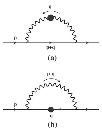
Figure 1: Resummed one-loop hard fermion self-energy with (a) soft internal photon and (b) soft internal fermion. The line with a dot denotes the HTL-resummed propagator.

III.2 Resummed one-loop self-energy of hard fermions

For massless fermions, it proves convenient to decompose the self-energy into positive and negative helicity components as

$$\Sigma(p_{0},p)=\gamma_{-}(\widehat{\mathbf{p}})\;\Sigma_{+}(p_{0},p)+\gamma_{+}(\widehat{\mathbf{p}})\;\Sigma_{-}(p_{0},p)\quad,\quad\Sigma_{\pm}(p_{0},p)=\frac{1}{2}\mathrm{Tr}[\gamma_{\pm}(\widehat{\mathbf{p}})\;\Sigma(p_{0},p)]\;,$$ (35)

where $\gamma_{\pm}(\widehat{\mathbf{p}})=(\gamma^{0}\mp\bm{\gamma}\cdot\widehat{\mathbf{p}})/2$ are the positive and negative helicity projectors, respectively. The resummed one-loop self-energy $\Sigma(P)$ of a hard fermion with momentum $p\sim T$, as depicted in Fig. 1, it receives contributions arising from soft internal photon and soft internal fermion lines. Let us write

$$\Sigma(P)=\Sigma^{\mathrm{sp}}(P)+\Sigma^{\mathrm{sf}}(P)\;,$$ (36)

where the superscripts ‘sp’ and ‘sf’ denote the soft-photon and soft-fermion contributions, respectively. Using the imaginary time propagators given in Appendix A, we find

$$\Sigma^{\mathrm{sp}}(P) = e^{2}\;T\sum_{\nu_{n}}\int\frac{d^{3}q}{(2\pi)^{3}}[\gamma^{0}\;S(P+Q)\gamma^{0}\;{}^{\ast}\!D_{L}(Q)+\gamma^{i}\;S(P+Q)\;\gamma^{j}\;{}^{\ast}\!D_{T}(Q)\;\mathcal{P}_{T}^{ij}(\widehat{\mathbf{q}})]\;,$$ (37)

$$\Sigma^{\mathrm{sf}}(P) = e^{2}\;T\sum_{\omega_{n}}\int\frac{d^{3}q}{(2\pi)^{3}}[\gamma^{0}\;{}^{\ast}\!S(Q^{\prime})\;\gamma^{0}\;D_{L}(P-Q^{\prime})+\gamma^{i}\;{}^{\ast}\!S(Q^{\prime})\;\gamma^{j}\;D_{T}(P-Q^{\prime})\;\mathcal{P}_{T}^{ij}(\widehat{\mathbf{p}-\mathbf{q}})]\;,$$ (38)

where $P=(i\omega_{m},\mathbf{p})$ with $p\sim T$, $Q=(i\nu_{n},\mathbf{q})$, $Q^{\prime}=(i\omega_{n},\mathbf{q})$ with $q\ll T$, and $\mathcal{P}_{T}^{ij}(\widehat{\mathbf{q}})=\delta^{ij}-\hat{q}^{i}\hat{q}^{j}$ is the transverse projector. For later convenience, we have assigned the loop momentum $Q$ to the soft internal propagators. Furthermore, we will neglect the instantaneous Coulomb interaction here and henceforth since it does not contribute to the imaginary part. After performing the Matsubara frequency sums, we can rewrite the self-energy as a spectral representation

$$\Sigma(i\omega_{m},p)=\int^{+\infty}_{-\infty}\frac{dp_{0}}{\pi}\;\frac{\mathrm{Im}\Sigma(p_{0},p)}{p_{0}-i\omega_{m}}\;,$$ (39)

This spectral representation will be useful to carry out the Matsubara sums when the self-energy is inserted in the polarization. Decomposing $\mathrm{Im}\Sigma(p_{0},p)$ onto $\gamma_{\pm}(\mathbf{p})$ analogous to eq. (35) and using the properties (see Appendix A for the spectral densities) ${}^{\ast}\!\rho_{L,T}(-q_{0},q)=-{}^{\ast}\!\rho_{L,T}(q_{0},q)$, ${}^{\ast}\!\rho_{\pm}(-q_{0},q)={}^{\ast}\!\rho_{\mp}(q_{0},q)$, $n_{B}(-q_{0})=-[1+n_{B}(q_{0})]$ and $n_{F}(-q_{0})=1-n_{F}(q_{0})$, we obtain

$$\mathrm{Im}\Sigma_{\pm}(p_{0},p)=\mathrm{Im}\Sigma^{\mathrm{sp}}_{\pm}(p_{0},p)+\mathrm{Im}\Sigma^{\mathrm{sf}}_{\pm}(p_{0},p)\;,$$ (40)

where

$$\mathrm{Im}\Sigma^{\mathrm{sp}}_{\pm}(p_{0},p) = \pi e^{2}\int\frac{d^{3}q}{(2\pi)^{3}}\int^{+\infty}_{-\infty}dq_{0}\;[n_{B}(q_{0})+n_{F}(|\mathbf{p}+\mathbf{q}|)]$$ (41)

$$\times\bigl{\{}\big{[}K^{\pm}_{1}(\mathbf{p},\mathbf{q})\;{}^{\ast}\!\rho_{L}(q_{0},q)+K^{\pm}_{2}(\mathbf{p},\mathbf{q})\;{}^{\ast}\!\rho_{T}(q_{0},q)\big{]}\;\delta(p_{0}+q_{0}-|\mathbf{p}+\mathbf{q}|)$$

$$+\big{[}K^{\mp}_{1}(\mathbf{p},\mathbf{q})\;{}^{\ast}\!\rho_{L}(q_{0},q)+K^{\mp}_{2}(\mathbf{p},\mathbf{q})\;{}^{\ast}\!\rho_{T}(q_{0},q)\big{]}\;\delta(p_{0}-q_{0}+|\mathbf{p}+\mathbf{q}|)\bigr{\}}\;,$$

$$\mathrm{Im}\Sigma^{\mathrm{sf}}_{\pm}(p_{0},p) = \pi e^{2}\int\frac{d^{3}q}{(2\pi)^{3}}\int^{+\infty}_{-\infty}dq_{0}\frac{1+n_{B}(|\mathbf{p}-\mathbf{q}|)-n_{F}(q_{0})}{2|\mathbf{p}-\mathbf{q}|}$$ (42)

$$\times\big{[}K^{\pm}_{3}(\mathbf{p},\mathbf{q})\;{}^{\ast}\!\rho_{+}(q_{0},q)+K^{\mp}_{3}(\mathbf{p},\mathbf{q})\;{}^{\ast}\!\rho_{-}(q_{0},q)\big{]}\;\delta(p_{0}-q_{0}-|\mathbf{p}+\mathbf{q}|)$$

$$+\big{[}K^{\mp}_{3}(\mathbf{p},\mathbf{q})\;{}^{\ast}\!\rho_{+}(q_{0},q)+K^{\pm}_{3}(\mathbf{p},\mathbf{q})\;{}^{\ast}\!\rho_{-}(q_{0},q)\big{]}\;\delta(p_{0}+q_{0}+|\mathbf{p}+\mathbf{q}|)\big{\}}\;,$$

with

$$K^{\pm}_{1}(\mathbf{p},\mathbf{q}) = \frac{1}{2}\;[1\pm\widehat{\mathbf{p}}\cdot\widehat{\mathbf{p}+\mathbf{q}}]\;,\;K^{\pm}_{2}(\mathbf{p},\mathbf{q})=1\mp(\widehat{\mathbf{p}}\cdot\widehat{\mathbf{q}})(\widehat{\mathbf{p}+\mathbf{q}}\cdot\widehat{\mathbf{q}})\;,\;K^{\pm}_{3}(\mathbf{p},\mathbf{q})=1\mp(\widehat{\mathbf{p}}\cdot\widehat{\mathbf{p}-\mathbf{q}})(\widehat{\mathbf{q}}\cdot\widehat{\mathbf{p}-\mathbf{q}})\;.$$ (43)

¿From the above expressions, one finds that $\mathrm{Im}\Sigma_{\pm}(-p_{0},p)=\mathrm{Im}\Sigma_{\mp}(p_{0},p)$. If $\mathrm{Im}\Sigma(p_{0},p)$ is finite on the particle and antiparticle mass shells $p_{0}=\pm p$, respectively, then $\Gamma(p)=\mathrm{Im}\Sigma_{\pm}(\pm p,p)$ is the damping rate for the hard (anti)fermion book:lebellac .

III.3 Anomalous damping of fermions

The leading contribution to the imaginary part of the hard fermion self-energy arises from the ultrasoft region of the transverse photon exchange for which $q\ll eT$ blaizot ; boyanqed ; scalar . This is so because in a high temperature QED plasma the fermionic excitation receives an effective thermal mass $m_{f}=eT/\sqrt{8}$ and the instantaneous Coulomb interaction is Debye screened by the electric (or Debye) mass $\omega_{D}=eT/\sqrt{3}$, whereas the magnetic interaction is only dynamically screened by Landau damping. Hence, we will focus only on the soft-photon contribution $\mathrm{Im}\Sigma^{\mathrm{sp}}_{\pm}$ in this subsection.

In the ultrasoft region of the loop momentum $q$, $q_{0}\ll eT$ in eq. (41), we can approximate the distribution $n_{B}(q_{0})+n_{F}(|\mathbf{p}+\mathbf{q}|)\simeq T/q_{0}$ and the HTL spectral function for the transverse photon blaizot ; boyanqed ; scalar

$$\frac{{}^{\ast}\!\rho_{T}(q_{0},q)}{q_{0}}\simeq\frac{\delta(q_{0})}{q^{2}}\;,$$ (44)

which as pointed out in Ref. blaizot can be interpreted as the exchange of a magnetostatic transverse photon. Furthermore, in this ultrasoft limit and for hard fermion momentum $p\gtrsim T$ we can replace $\widehat{\mathbf{p}+\mathbf{q}}\simeq\widehat{\mathbf{p}}$. After some algebra, we find near the particle and antiparticle mass shells $p_{0}\sim\pm p$ blaizot ; boyanqed

$$\mathrm{Im}\Sigma^{\mathrm{sp}}_{\pm}(p_{0}\approx\pm p,p)=\alpha T\int^{\omega_{D}}_{0}dq\int_{-1}^{1}dx\;(1-x^{2})\;\delta(p_{0}\mp p-qx)\;,$$ (45)

where $x=\widehat{\mathbf{p}}\cdot\widehat{\mathbf{q}}$. The integration is straightforward and yields the following leading order result

$$\mathrm{Im}\Sigma^{\mathrm{sp}}_{\pm}(p_{0}\approx\pm p,p)=\alpha T\ln\left|\frac{\omega_{D}}{p_{0}\mp p}\right|+{\cal O}\left(|{p_{0}\mp p}|^{0}\right)\;.$$ (46)

While the fermion damping rate is ill-defined, several resummation schemes, either based on the thermal eikonal (Bloch-Nordsieck) approximation that sums rainbow diagrams blaizot or via the dynamical renormalization group boyanqed ; scalar , lead to the conclusion that the fermion propagator at large times decays in real time as

$$\langle\Psi(\mathbf{x}{},t{})\bar{\Psi}(\mathbf{0},0)\rangle\propto e^{-\alpha\;T\;t\;\ln(\omega_{D}t)}\;,$$ (47)

which corresponds to an inverse relaxation time scale for the hard fermion

$$\Gamma=\alpha\;T\;\ln(1/e)\;.$$ (48)

This is known as the anomalous fermion damping lebedev and is determined by the kinematic region of ultrasoft transverse photon exchange with momentum $q\ll eT$. The region $q\gtrsim eT$ of transverse photon exchange leads to a subleading contribution to the damping of hard fermions of the order $\alpha^{2}T$ blaizot ; basagoiti2 ; aarts .

The reasons to repeat this analysis here are twofold: (i) to clarify in real time that the anomalous damping rate eq. (48) does not contribute to the conductivity, as a consequence of a cancellation between self-energy and vertex corrections as anticipated in Ref. lebedev , and (ii) we will study the solution of the Boltzmann equation in the relaxation time approximation which will also feature the anomalous time dependence.

As it will be discussed in detail below in Sec. IV.4, there is a precise cancellation of the contribution from ultrasoft photon momentum exchange between the self-energy and the vertex corrections to the polarization in perturbation theory. This cancellation will also be manifest in the linearized Boltzmann equation, and the analysis presented above will lead us to a direct identification of self-energy and vertex contributions in the linearized Boltzmann equation.

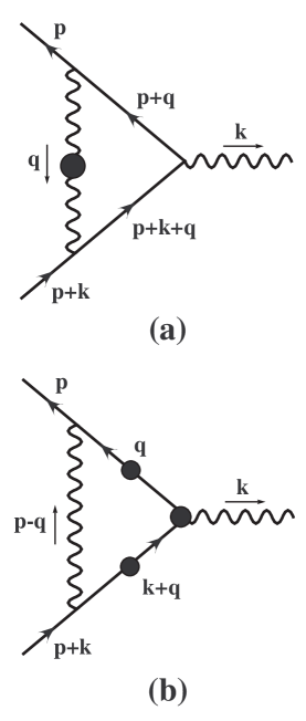
Figure 2: Resummed one-loop hard fermion-soft photon vertex with (a) soft internal photon and (b) soft internal fermion. The line (vertex) with a dot denotes the HTL-resummed propagator (vertex).

III.4 Resummed one-loop fermion-photon vertex

We now evaluate the resummed one-loop hard fermion-soft photon vertex, which consistently with the Ward identityaarts also receives contributions from soft internal photon and soft internal fermion (see Fig. 2). Writing,

$$\Gamma^{\mu}(P+K,P)=\Gamma^{\mathrm{sp},\mu}(P+K,P)+\Gamma^{\mathrm{sf},\mu}(P+K,P)\;,$$ (49)

we find in the imaginary time formalism,

$$e\;\Gamma^{\mathrm{sp},\mu}(P+K,P) = e^{3}\;T\sum_{\nu_{n}}\int\frac{d^{3}q}{(2\pi)^{3}}\,\big{[}\gamma^{0}\;S(P+Q)\;\gamma^{\mu}\;S(P+K+Q)\;\gamma^{0}\;{}^{\ast}\!D_{L}(Q)+$$ (50)

$$+\,\gamma^{i}\;S(P+Q)\;\gamma^{\mu}\;S(P+K+Q)\;\gamma^{j}\;{}^{\ast}\!D_{T}(Q)\;\mathcal{P}_{T}^{ij}(\widehat{\mathbf{q}})\big{]}\;,$$

$$e\;\Gamma^{\mathrm{sf},\mu}(P+K,P) = e^{3}\;T\sum_{\omega_{n}}\int\frac{d^{3}q}{(2\pi)^{3}}\,\big{[}\gamma^{0}\;{}^{\ast}\!S(Q^{\prime})\;{}^{\ast}\Gamma^{\mu}(Q^{\prime}+K,Q^{\prime})\;{}^{\ast}\!S(Q^{\prime}+K)\;\gamma^{0}\;D_{L}(P-Q^{\prime})+$$ (51)

$$+\,\gamma^{i}\;{}^{\ast}\!S(Q^{\prime})\;{}^{\ast}\Gamma^{\mu}(Q^{\prime}+K,Q^{\prime})\;{}^{\ast}\!S(Q^{\prime}+K)\;\gamma^{j}\;D_{T}(P-Q)\;\mathcal{P}_{T}^{ij}(\widehat{\mathbf{p}-\mathbf{q}})\big{]}\;,$$

where ${}^{\ast}\Gamma^{\mu}$ is the HTL-resummed fermion-photon vertex, $K=(i\nu_{k},\mathbf{k})$ with $k\ll T$, and the rest of the four-momenta are the same as those defined for the self-energy.

Indeed, using the Ward identities satisfied by the respective free and HTL-resummed quantities book:lebellac

$$K_{\mu}\gamma^{\mu}=S^{-1}(Q)-S^{-1}(K+Q)\;,\quad K_{\mu}\;{}^{\ast}\Gamma^{\mu}(Q^{\prime}+K,Q^{\prime})={}^{\ast}\!S^{-1}(Q^{\prime})-{}^{\ast}\!S^{-1}(Q^{\prime}+K)\;,$$ (52)

and the expressions for the vertices given by eqs. (50) and (51), one can easily show that the resummed one-loop self-energy and vertex satisfy the Ward identities

$$K_{\mu}\;\Gamma^{\mathrm{sp},\mu}(P+K,P)=\Sigma^{\mathrm{sp}}(P+K)-\Sigma^{\mathrm{sp}}(P)\;,\quad K_{\mu}\;\Gamma^{\mathrm{sf},\mu}(P+K,P)=\Sigma^{\mathrm{sf}}(P+K)-\Sigma^{\mathrm{sf}}(P)\;,$$ (53)

hence

$$K_{\mu}\;\Gamma^{\mu}(P+K,P)=\Sigma(P+K)-\Sigma(P).$$ (54)

We note that these Ward identities for the resummed one-loop self-energy and vertex are exact in the kinematic region under consideration $p\sim T$ and $k\ll T$.

Let us first concentrate on the soft-photon contribution $\Gamma^{\mathrm{sp},\mu}$. The sum over the Matsubara frequencies can be done straightforwardly. Using the identity

$$\frac{1}{ab}=\mathrm{PV}\left(\frac{1}{b-a}\right)\left(\frac{1}{a}-\frac{1}{b}\right),$$ (55)

where the principal value (PV) prescription is necessary to define the limit $b-a\to 0$, we find that,

$$\Gamma^{\mathrm{sp},\mu}(P+K,P) = e^{2}\int\frac{d^{3}q}{(2\pi)^{3}}\int^{+\infty}_{-\infty}dq_{0}\int^{+\infty}_{-\infty}dp_{0}\int^{+\infty}_{-\infty}ds_{0}\big{[}\gamma^{i}\;\rho_{F}(p_{0},\mathbf{p}+\mathbf{q})\;\gamma^{\mu}\;\rho_{F}(s_{0},\mathbf{p}+\mathbf{k}+\mathbf{q})\;\gamma^{j}\;$$ (56)

$$\times\,{}^{\ast}\!\rho_{T}(q_{0},q)\;\mathcal{P}_{T}^{ij}(\widehat{\mathbf{q}})+\gamma^{0}\;\rho_{F}(p_{0},\mathbf{p}+\mathbf{q})\;\gamma^{\mu}\;\rho_{F}(s_{0},\mathbf{p}+\mathbf{k}+\mathbf{q})\gamma^{0}\;{}^{\ast}\!\rho_{L}(q_{0},q)\big{]}$$

$$\times\,\frac{1}{s_{0}-p_{0}-i\nu_{k}}\left[\frac{n_{B}(q_{0})+n_{F}(p_{0})}{p_{0}-q_{0}-i\omega_{m}}-\frac{n_{B}(q_{0})+n_{F}(s_{0})}{s_{0}-q_{0}-i\omega_{m}-i\nu_{k}}\right]\;,$$

where the denominator $1/(s_{0}-p_{0}-i\nu_{k})$ in the above expression should be understood with the principal value prescription as in eq. (55).

The kinematic region of interest for the polarization and the conductivity corresponds to hard external fermion $p\sim T$ and soft external photon $k\ll T$. Furthermore after the analytic continuation of the external photon frequency $i\nu_{k}\to\omega+i0$ we need $\omega\ll T$, and eventually we will take the long-wavelength, low-frequency limit $\omega,k\to 0$.

The form of the free fermion spectral function $\rho_{F}$ suggests that the above result can be written as a sum of the products $\rho_{+}\;\rho_{+}$, $\rho_{-}\;\rho_{-}$, $\rho_{+}\;\rho_{-}$ and $\rho_{-}\;\rho_{+}$, where $\rho_{\pm}$ are the respective spectral functions for free fermion and antifermion [see eq. (187)]. The integrals over the dispersive variables $p_{0}$ and $s_{0}$ can be done trivially using the spectral functions for free fermions. For hard external fermion $p\sim T$ and soft external photon $k\ll T$ we can make the following kinematic approximations

$$|\mathbf{p}+\mathbf{k}+\mathbf{q}|-|\mathbf{p}+\mathbf{q}| \simeq \widehat{\mathbf{p}+\mathbf{q}}\cdot\mathbf{k}\sim k\;,\quad|\mathbf{p}+\mathbf{k}+\mathbf{q}|+|\mathbf{p}+\mathbf{q}|\simeq 2|\mathbf{p}+\mathbf{q}|\sim T\;.$$ (57)

After the analytic continuation of the external photon frequency $i\nu_{k}\to\omega+i0$ with $\omega\sim k\ll T$, we find the products $\rho_{\pm}\rho_{\pm}$ lead to denominators of the form

$$\frac{1}{\widehat{\mathbf{p}+\mathbf{q}}\cdot\mathbf{k}\mp\omega}\;,$$ (58)

whereas the products $\rho_{\pm}\rho_{\mp}$ lead to denominators of the form

$$\frac{1}{2|\mathbf{p}+\mathbf{q}|\mp\omega}\sim\frac{1}{T}\;.$$ (59)

Hence in the long-wavelength, low-frequency (or hydrodynamic) limit of the external photon $k$, $\omega\to 0$, the products $\rho_{\pm}\rho_{\pm}$ lead to singular denominators (pinch singularities) which furnish the leading contributions, whereas products of the form $\rho_{\pm}\rho_{\mp}$ lead to contributions that are suppressed by inverse powers of the temperature. We note that in our notation the pole-like singularities of the form given by eq. (58) must be understood with a principal value prescription as discussed above. Since these poles emerge in the hydrodynamic limit and play an important role in our discussion below, hereafter we will refer to them as hydrodynamic poles.

Keeping only terms with the products $\rho_{\pm}\rho_{\pm}$ that eventually lead to hydrodynamic poles, we find after some algebra that $\Gamma^{\mathrm{sp},\mu}(P+K,P)$ in the hydrodynamic limit can be written in the spectral representation as

$$\Gamma^{\mathrm{sp},\mu}(P+K,P)=\int^{+\infty}_{-\infty}ds_{0}\left[\frac{\digamma^{\mu}(s_{0},\mathbf{p};i\nu_{k},\mathbf{k})}{s_{0}-i\omega_{m}}-\frac{\digamma^{\mu}(s_{0},\mathbf{p}+\mathbf{k};i\nu_{k},\mathbf{k})}{s_{0}-i\omega_{m}-i\nu_{k}}\right]\;,$$ (60)

where

$$\digamma^{\mu}(s_{0},\mathbf{p};k_{0},\mathbf{k})=\gamma_{-}(\widehat{\mathbf{p}})\;\digamma_{+}^{\mu}(s_{0},\mathbf{p};k_{0},\mathbf{k})+\gamma_{+}(\widehat{\mathbf{p}})\;\digamma_{-}^{\mu}(s_{0},\mathbf{p};k_{0},\mathbf{k})\;.$$ (61)

The components $\digamma_{\pm}^{\mu}$ are given by

$$\digamma_{\pm}^{\mu}(s_{0},\mathbf{p};i\nu_{k},\mathbf{k}) = e^{2}\int\frac{d^{3}q}{(2\pi)^{3}}\int^{+\infty}_{-\infty}dq_{0}\,\bigg{\{}\frac{L^{\mu}_{+}(\widehat{\mathbf{p}+\mathbf{q}})}{\widehat{\mathbf{p}+\mathbf{q}}\cdot\mathbf{k}-i\nu_{k}}\big{[}K^{\pm}_{1}(\mathbf{p},\mathbf{q})\;{}^{\ast}\!\rho_{L}(q_{0},q)+K^{\pm}_{2}(\mathbf{p},\mathbf{q})\;{}^{\ast}\!\rho_{T}(q_{0},q)\big{]}$$ (62)

$$\times\,\delta(|\mathbf{p}+\mathbf{q}|-q_{0}-s_{0})-\frac{L^{\mu}_{-}(\widehat{\mathbf{p}+\mathbf{q}})}{\widehat{\mathbf{p}+\mathbf{q}}\cdot\mathbf{k}+i\nu_{k}}\big{[}K^{\mp}_{1}(\mathbf{p},\mathbf{q})\;{}^{\ast}\!\rho_{L}(q_{0},q)+K^{\mp}_{2}(\mathbf{p},\mathbf{q})\;{}^{\ast}\!\rho_{T}(q_{0},q)\big{]}$$

$$\times\,\delta(|\mathbf{p}+\mathbf{q}|-q_{0}+s_{0})\bigg{\}}\;[n_{B}(q_{0})+n_{F}(|\mathbf{p}+\mathbf{q}|)]\;,$$

with $L_{\pm}(\widehat{\mathbf{p}})=(1,\pm\widehat{\mathbf{p}})$ being lightlike four-vectors.

The soft-fermion contribution to the vertex has been studied in detail in Ref. aarts . The conclusion of the detailed study of the vertex is that whereas the soft-fermion contribution is needed to fulfill the Ward identity, its contribution to the polarization is subleading aarts . Anticipating that in agreement with this conclusion that the soft-fermion contribution to the vertex will not contribute at leading logarithmic order, we will neglect this contribution for the moment and postpone a detailed discussion until we study the vertex corrections to the resummed two-loop photon polarization (see Sec. IV.3).

III.5 Resummed one-loop Ward identity in the hydrodynamic limit

In the program that we advocate here, namely the implementation of a resummation of the secular terms via the dynamical renormalization group in real time, we must confirm that the main ingredients in such a resummation fulfill the Ward identity, which guarantees that the result of the resummation will be gauge invariant.

While eqs. (52)-(53) and (54) assert the fulfillment of the Ward identities, our focus below will be to extract the secular terms that are associated with hydrodynamic poles of the form $(\mathbf{k}\cdot\widehat{\mathbf{p}}-\omega)^{-n}$ in the limit $\mathbf{k};\omega\rightarrow 0$. These poles are the manifestation of the pinch singularities and in real time they lead to secular terms in the perturbative expansion as discussed above. To lowest order with HTL resummed propagators these poles correspond to $n=1,2$. As it will become clear in the detailed discussion below, the dynamical renormalization group will provide a resummation of the leading order secular terms. Thus the building blocks of the resummation program are precisely these singular terms arising from the insertions of one loop self-energy and vertex with HTL resummed propagators.

Thus we must confirm that the Ward identity between the resummed one-loop self-energy and vertex is fulfilled for these singular contributions. Once the Ward identity of these building blocks is confirmed, the dynamical renormalization group program that leads to a resummation of these leading order singular contribution is gauge invariant.

As per the discussion above we will neglect the soft-fermion contribution to the vertex in the analysis that follows since its contribution to the polarization is subleading aarts (see below). The spectral representation of $\Gamma^{\mathrm{sp},\mu}$ given by eqs. (60)–(62) is particularly useful to establish the Ward identity between the resummed one-loop self-energy and vertex in the hydrodynamic limit. With the spectral representation for the self-energy eq. (39) in terms of $\mathrm{Im}\Sigma^{\mathrm{sp}}$ given by eq. (41) and the above spectral representation for the vertex $\Gamma^{\mathrm{sp},\mu}$, it is straightforward to check that the resummed one-loop Ward identity

$$K_{\mu}\Gamma^{\mathrm{sp},\mu}(P+K,P)=\int^{+\infty}_{-\infty}\frac{ds_{0}}{\pi}\bigg{[}\frac{\mathrm{Im}\Sigma^{\mathrm{sp}}(s_{0},\mathbf{p}+\mathbf{k})}{s_{0}-i\omega_{m}-i\nu_{k}}-\frac{\mathrm{Im}\Sigma^{\mathrm{sp}}(s_{0},\mathbf{p})}{s_{0}-i\omega_{m}}\bigg{]}=\Sigma^{\mathrm{sp}}(P+K)-\Sigma^{\mathrm{sp}}(P)$$ (63)

is fulfilled in the hydrodynamic limit. The next step in the program is to insert the resummed one-loop self-energy and vertex in the transverse photon polarization, the fulfillment of the Ward identity between the self-energy and the vertex will ensure current conservation and gauge invariance.

IV Resummed two-loop transverse photon polarization

At two-loop order the calculation of the photon self-energy involves two kinds of topologically different diagrams, namely the self-energy and vertex correction diagrams as depicted in Figs. 3 and 4, respectively. Similar diagrams have been studied for a hot QCD plasma within the context of photon or dilepton production diagrams and more recently in Ref. gale but in a very different kinematic region. The color algebra, which introduces important differences, and the very different kinematic region of interest for dilepton production, which is not the relevant for transport phenomena, make these previous calculations not useful for the purpose of studying transport coefficients in the hot QED plasma.

IV.1 The self-energy contribution

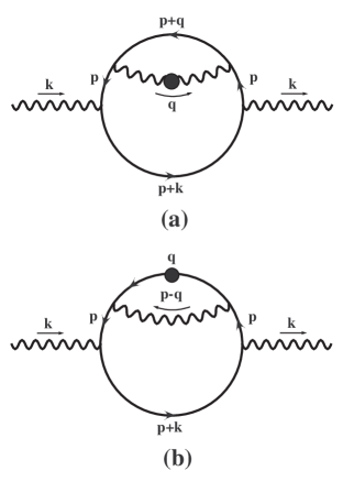
Figure 3: Resummed two-loop photon polarization with the fermion self-energy correction.

The two-loop diagrams for the fermion self-energy contribution to the transverse polarization are depicted in Fig. 3. In the imaginary-time formalism the self-energy correction to the polarization is given by

$$\Pi^{\mathrm{SE},ij}(K)=e^{2}T\sum_{\omega_{m}}\mathrm{Tr}\int\frac{d^{3}p}{(2\pi)^{3}}\;[\gamma^{i}\;S(P)\;\Sigma(P)\;S(P)\;\gamma^{j}\;S(P+K)+\gamma^{i}\;S(P)\;\gamma^{j}\;S(P+K)\;\Sigma(P+K)\;S(P+K)]\;,$$ (64)

where $\Sigma(P)$ is one-loop resummed fermion self-energy in the spectral representation given by eq. (39) and for later convenience we have written down explicitly the self-energy insertion for each fermion line. The Matsubara sum over the internal fermion frequency can be performed easily following the method illustrated in the previous section. After using the identity eq. (55) we obtain

$$\Pi^{\mathrm{SE},ij}(K) = \frac{e^{2}}{\pi}\,\mathrm{Tr}\int\frac{d^{3}p}{(2\pi)^{3}}\int^{+\infty}_{-\infty}dp_{0}\int^{+\infty}_{-\infty}dq_{0}\int^{+\infty}_{-\infty}ds_{0}\int^{+\infty}_{-\infty}dt_{0}\bigg{\{}\gamma^{i}\;\rho_{F}(p_{0},\mathbf{p})\;\mathrm{Im}\Sigma(q_{0},p)\;\rho_{F}(s_{0},\mathbf{p})\;\gamma^{j}$$ (65)

$$\times\,\rho_{F}(t_{0},\mathbf{p}+\mathbf{k})\bigg{[}\frac{n_{F}(t_{0})-n_{F}(p_{0})}{(p_{0}-s_{0})(p_{0}-q_{0})(t_{0}-p_{0}-i\nu_{k})}+\frac{n_{F}(t_{0})-n_{F}(s_{0})}{(s_{0}-p_{0})(s_{0}-q_{0})(t_{0}-s_{0}-i\nu_{k})}+$$

$$+\,\frac{n_{F}(t_{0})-n_{F}(q_{0})}{(q_{0}-p_{0})(q_{0}-s_{0})(t_{0}-q_{0}-i\nu_{k})}\bigg{]}+\gamma^{i}\;\rho_{F}(t_{0},\mathbf{p})\;\gamma^{j}\;\rho_{F}(p_{0},\mathbf{p}+\mathbf{k})\;\mathrm{Im}\Sigma(q_{0},p+k)$$

$$\times\,\rho_{F}(s_{0},\mathbf{p}+\mathbf{k})\bigg{[}\frac{n_{F}(t_{0})-n_{F}(p_{0})}{(p_{0}-s_{0})(p_{0}-q_{0})(t_{0}-p_{0}+i\nu_{k})}+\frac{n_{F}(t_{0})-n_{F}(s_{0})}{(s_{0}-p_{0})(s_{0}-q_{0})(t_{0}-s_{0}+i\nu_{k})}+$$

$$+\,\frac{n_{F}(t_{0})-n_{F}(q_{0})}{(q_{0}-p_{0})(q_{0}-s_{0})(t_{0}-q_{0}+i\nu_{k})}\bigg{]}\bigg{\}}\;,$$

where $\mathrm{Im}\Sigma(q_{0},p)$ is given by eq. (40) and all the frequency denominators are understood with the principal value prescription.

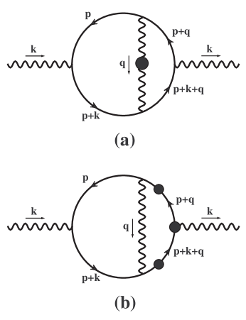
Figure 4: Resummed two-loop photon polarization with the fermion-photon vertex correction.

The imaginary part $\mathrm{Im}\Pi^{\mathrm{SE},ij}(\omega,k)$ is obtained through the analytical continuation $i\nu_{k}\to\omega+i0$ and can be interpreted as cutting the photon self-energy diagrams in Fig. 3 in all possible manners. However, just as in the discussion of the vertex above, terms with products of the form $\rho_{\pm}\rho_{\pm}\rho_{\pm}$ give the leading contributions that feature hydrodynamic poles (or pinch denominators) in the hydrodynamic limit, while terms that involve mixed products of $\rho_{\pm}$ will be subleading by powers of $1/T$. Therefore, only the products with the same particle or antiparticle components in all fermionic lines will yield the leading contribution.

Focusing only on the leading contributions arising from terms where the fermion spectral functions are either all particle ($\rho_{+}$) or all antiparticle ($\rho_{-}$) [see eq. (187)], we find

$$\mathrm{Im}\Pi^{\mathrm{SE},ij}(\omega,k) = \pi e^{2}\,\mathrm{PV}\int\frac{d^{3}p}{(2\pi)^{3}}\int^{+\infty}_{-\infty}dp_{0}\int^{+\infty}_{-\infty}dq_{0}\int^{+\infty}_{-\infty}ds_{0}\int^{+\infty}_{-\infty}dt_{0}\;\frac{n_{F}(t_{0})-n_{F}(q_{0})}{(q_{0}-p_{0})(q_{0}-s_{0})}$$ (66)

$$\times\,\mathrm{Tr}\left[\gamma^{i}\;\rho_{F}(p_{0},\mathbf{p})\;\mathrm{Im}\Sigma(q_{0},p)\;\rho_{F}(s_{0},\mathbf{p})\;\gamma^{j}\;\rho_{F}(t_{0},\mathbf{p}+\mathbf{k})\;\delta(t_{0}-q_{0}-\omega)\right.$$

$$\left.-\,\gamma^{i}\;\rho_{F}(t_{0},\mathbf{p})\;\gamma^{j}\;\rho_{F}(p_{0},\mathbf{p}+\mathbf{k})\;\mathrm{Im}\Sigma(q_{0},p+k)\;\rho_{F}(s_{0},\mathbf{p}+\mathbf{k})\;\delta(t_{0}-q_{0}+\omega)\right]\;,$$

where the fermion spectral functions are either all particle or antiparticle contributions. Since the dispersive variable $q_{0}$ is constrained by the delta functions $\delta(t_{0}-q_{0}\mp\omega)$, the leading terms that feature hydrodynamic poles are obtained from cutting the polarization diagrams in Fig. 3 through the fermion self-energy and hence the internal soft photon line. The other possible cuts do not lead to hydrodynamic poles, hence no secular terms arise from the other cuts.

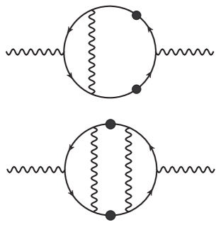
Figure 5: Diagrams corresponding to the resummed two-loop photon polarization in Fig. 4(b).

Performing the integrals over $p_{0}$, $q_{0}$, $s_{0}$, and $t_{0}$ by using the delta functions, we find the leading terms in $k$, $\omega\to 0$ limit to be given by

$$\mathrm{Im}\Pi^{\mathrm{SE},ij}(\omega,k)=2\pi\;e^{2}\;\omega\;\mathrm{PV}\int\frac{d^{3}p}{(2\pi)^{3}}\frac{dn_{F}(p)}{dp}\;\hat{p}^{i}\;\hat{p}^{j}\;\bigg{[}\frac{\mathrm{Im}\Sigma_{+}(|\mathbf{p}+\mathbf{k}|-\omega,p)+\mathrm{Im}\Sigma_{+}(p+\omega,|\mathbf{p}+\mathbf{k}|)}{(\mathbf{k}\cdot\widehat{\mathbf{p}}-\omega)^{2}}+(\omega\to-\omega)\bigg{]}\;,$$ (67)

where we have used the property $\mathrm{Im}\Sigma_{-}(-\omega,p)=\mathrm{Im}\Sigma_{+}(\omega,p)$. The above expression shows clearly that in $k$, $\omega\to 0$ limit the leading contributions to $\mathrm{Im}\Pi^{\mathrm{SE},ij}(\omega,k)$ arise from terms that feature hydrodynamic poles of the form

$$\frac{1}{(\mathbf{k}\cdot\widehat{\mathbf{p}}\mp\omega)^{2}}.$$ (68)

which will lead to linear secular terms in time. For $k,\omega\ll p\sim T$ we see that the imaginary parts of the fermion self-energy in eq. (67) above are nearly on the mass shell of fermions or antifermions, the off-shellness being of order $|\omega-\mathbf{k}\cdot\widehat{\mathbf{p}}|$. Upon inserting $\mathrm{Im}\Sigma_{+}$ given by eq. (41) into eq. (67) and noticing that for $q\ll T$ the second delta functions in eq. (41) cannot be satisfied near the fermion mass shell, we obtain

$$\mathrm{Im}\Pi^{\mathrm{SE},ij}(\omega,k)=2\pi^{2}e^{4}\omega\,\mathrm{PV}\int\frac{d^{3}p}{(2\pi)^{3}}\frac{dn_{F}(p)}{dp}\;\hat{p}^{i}\;\hat{p}^{j}\;\int\frac{d^{3}q}{(2\pi)^{3}}\int^{+\infty}_{-\infty}dq_{0}\;\bigg{\{}[n_{B}(q_{0})+n_{F}(|\mathbf{p}+\mathbf{q}|)]$$

$$\times\big{[}K^{+}_{1}(\mathbf{p},\mathbf{q})\;{}^{\ast}\!\rho_{L}(q_{0},q)+K^{+}_{2}(\mathbf{p},\mathbf{q})\;{}^{\ast}\!\rho_{T}(q_{0},q)\big{]}+\frac{1}{2|\mathbf{p}-\mathbf{q}|}[1+n_{B}(|\mathbf{p}-\mathbf{q}|)-n_{F}(q_{0})]$$ (69)

$$\times\,\big{[}K^{+}_{3}(\mathbf{p},\mathbf{q})\;{}^{\ast}\!\rho_{+}(q_{0},q)+K^{-}_{3}(\mathbf{p},\mathbf{q})\;{}^{\ast}\!\rho_{-}(q_{0},q)\big{]}\bigg{\}}\bigg{[}\frac{\delta(\widehat{\mathbf{p}}\cdot\mathbf{q}-q_{0}-\mathbf{k}\cdot\widehat{\mathbf{p}}+\omega)+\delta(\widehat{\mathbf{p}}\cdot\mathbf{q}-q_{0}+\mathbf{k}\cdot\widehat{\mathbf{p}}-\omega)}{(\mathbf{k}\cdot\widehat{\mathbf{p}}-\omega)^{2}}+(\omega\to-\omega)\bigg{]}\;.$$

As will be shown below, the hydrodynamic poles in $\mathrm{Im}\Pi^{\mathrm{SE},ij}(\omega,k)$ correspond to secular terms in time in the function $\mathcal{G}^{ij}(t)$ and signal the need for resummation in real time.

IV.2 Anomalous secular term from the self-energy

At this stage we can begin establishing a connection with the program of resummation in real time by analyzing the leading secular terms arising in the perturbative expansion. As analyzed in detail in Sec. III.3, the leading contribution to the imaginary part of the self-energy near the fermion (or antifermion) mass shell is determined by the exchange of an ultrasoft transverse photon with momentum $q\ll eT$. Keeping only this leading contribution for the moment, we find that for $k\ll p$ [see eq. (46)]

$$\mathrm{Im}\Sigma^{\mathrm{sp}}_{+}(|\mathbf{p}+\mathbf{k}|-\omega,p)=\mathrm{Im}\Sigma^{\mathrm{sp}}_{+}(p+\omega,|\mathbf{p}+\mathbf{k}|)=-\alpha\;T\;\ln\left|\frac{\omega-\mathbf{k}\cdot\widehat{\mathbf{p}}}{\omega_{D}}\right|\;.$$ (70)

Introducing this leading estimate for the imaginary part of the fermion (antifermion) self-energy into eq. (67), we obtain

$$\mathrm{Im}\Pi^{\mathrm{SE},ij}(\omega,k)=-4e^{2}\alpha T\omega\,\mathrm{PV}\int\frac{d^{3}p}{(2\pi)^{3}}\frac{dn_{F}(p)}{dp}\left[\frac{\hat{p}^{i}\hat{p}^{j}}{(\omega-\mathbf{k}\cdot\widehat{\mathbf{p}})^{2}}\ln\left|\frac{\omega-\mathbf{k}\cdot\widehat{\mathbf{p}}}{\omega_{D}}\right|+(\omega\to-\omega)\right]\;.$$ (71)

We now compute the function $\mathcal{G}^{ij}(k,t)$ by performing the Fourier transform in $\omega$ as per eq. (10). Using the properties of the principal value, we find

$$\mathcal{G}^{\mathrm{SE},ij}(t)=-2\alpha\,\mathcal{G}^{\mathrm{HTL},ij}\int^{+\infty}_{-\infty}\frac{1-\cos(yt)}{\pi y^{2}}\;\ln\left|\frac{y}{\omega_{D}}\right|\;,$$ (72)

where $\mathcal{G}^{\mathrm{HTL},ij}(t)$ is given by eq. (33). With the help of the results established in Refs. boyanqed ; scalar , we find the asymptotic long time limit to be given by

$$\mathcal{G}^{\mathrm{SE},ij}(t)=\mathcal{G}^{\mathrm{HTL},ij}\;\left[-2\alpha Tt\ln(\omega_{D}t)+\mathrm{non~{}secular~{}terms}\right]\;.$$ (73)

Therefore combining the one-loop (HTL) result with the leading contribution from ultrasoft transverse photon exchange in the resummed self-energy correction to the two-loop polarization, we find

$$\mathcal{G}^{ij}(t)=\mathcal{G}^{\mathrm{HTL},ij}\;\left[1-2\alpha Tt\ln(\omega_{D}t)+\mathrm{non~{}secular~{}terms}\right]\;.$$ (74)

Let us assume for a moment that the exponentiation of the leading secular term in the form

$$\mathcal{G}^{ij}(t)=\mathcal{G}^{\mathrm{HTL},ij}(t)\;e^{-2\alpha Tt\ln(\omega_{D}t)}=-\delta_{ij}\;\frac{e^{2}\,T^{2}}{9}\;e^{-2\alpha Tt\ln(\omega_{D}t)}\;,$$ (75)

and explore the consequences of this result. [We used here eq. (33)]. Such exponentiation would be justified considering only the self-energy insertion on both fermionic lines in the loop and on the basis of the resummed form of the propagator eq. (47) blaizot ; boyanqed since the function $\mathcal{G}(k,t)$ behaves as the square of the propagator. Furthermore, as it has become customary in the literature, let us approximate

$$e^{-2\alpha Tt\ln(\omega_{D}\;t)}\approx e^{-2\Gamma t}\;,$$ (76)

with the anomalous damping rate given by eq. (48). The time integral of $\mathcal{G}^{ij}(t)$ [see eq. (30)] to obtain the conductivity can now be done in closed form and we find

$$\sigma\approx\frac{e^{2}T^{2}}{18\,\Gamma}=\frac{2\pi}{9}\frac{T}{\ln(1/e)}+\mathrm{subleading}\;.$$ (77)

This discussion highlights several important points:

• In the limit $k$, $\omega\to 0$ the hydrodynamic poles of the form $1/(\omega\mp\mathbf{k}\cdot\widehat{\mathbf{p}})^{2}$, which are a consequence of the pinch terms jeon , result in secular perturbations for $\mathcal{G}(k,t)$, i.e., terms that grow in time. The relation between pinch singularities and secular terms in perturbative theory and their resummation via the dynamical renormalization group has been previously discussed in Refs. boyanqed ; scalar .

  ¿From eq. (72) and the results obtained in Refs. boyanqed ; scalar we see that the hydrodynamic pole $1/(\omega-\mathbf{k}\cdot\widehat{\mathbf{p}})^{2}$ leads to a secular term linear in $t$, while the threshold singularity $\ln|\omega-\mathbf{k}\cdot\widehat{\mathbf{p}}|$ leads to the $\ln(\omega_{D}\,t)$ enhancement of the secular term. Thus, the extra logarithmic contribution to the secular term originates in the ultrasoft momentum region $q\ll eT$ of the exchanged transverse photon, which is only dynamically screened by Landau damping. Without this infrared, logarithmic enhancement the hydrodynamic pole would lead to a secular term linear in time. This observation will be important when we combine the contributions from the self-energy and vertex.

• If the imaginary part of the fermion self-energy on the mass shell were a finite constant $\Gamma\ll T$ a Dyson resummation of self-energy insertions would lead to a Breit-Wigner form for the fermion and antifermion spectral functions near the mass shell, namely

  $$\rho_{\pm}(p_{0},p)=\frac{1}{\pi}\frac{\Gamma}{(p_{0}\mp p)^{2}+\Gamma^{2}}\;.$$ (78)

  Using these spectral functions to compute the imaginary part of the polarization to one-loop order, keeping only the products $\rho_{\pm}\;\rho_{\pm}$ and taking the limits $k$, $\omega\to 0$, it is straightforward to find that the conductivity is independent of these limits and given by

  $$\sigma=\frac{e^{2}T^{2}}{18\,\Gamma}\;.$$ (79)

  This simple exercise shows that the resummation of the secular terms in eq. (75) by taking the coefficient of $t$ to be a constant $2\Gamma$ gives the correct answer for the conductivity in the case where the damping rate is a finite constant and the spectral function near the quasiparticle poles is of the Breit-Wigner form, providing a reassuring check in a simpler case.

• In order to avoid confusion, we want to stress that the eqs. (77)-(79) are a result of the self-energy correction only. As will be discussed in detail below, the vertex correction cancels the ultrasoft photon exchange contribution from the self-energy and as a result the eqs. (77)-(79) do not apply to the hot QED plasma. The correct expression is given by eq. (185). The main point of the derivation of eqs. (77)-(79) is the following: (a) to illustrate what would be the result if only the self-energy correction is taken into account but without the vertex correction, (b) as we will show below that this approximation is equivalent to the relaxation time approximation in the Boltzmann equation.

As it will be seen in detail later when we implement the dynamical renormalization group the resummed form of $\mathcal{G}(t)$ with only self-energy correction is much more subtle than the simple exponentiation assumed above in eq. (75). While the result obtained above is correct for a constant damping rate, the anomalous logarithmic time dependence will prevent the existence of a drift current at long times leading to a vanishing conductivity from only self-energy corrections from ultrasoft photon exchange. We will discuss these issues in more detail in Sec. V.2, where we introduce the dynamical renormalization group equation in the relaxation time approximation.

While this discussion has highlighted these important points, keeping only the self-energy corrections is not consistent with the Ward identities and the vertex correction must be included. As advanced in Ref. lebedev and discussed explicitly below in Sec. IV.4, the contribution from the anomalous damping to the conductivity is in fact cancelled by the vertex correction. This cancellation, which will also be made manifest in the Boltzmann equation below is the reason that the conductivity is determined not by the quasiparticle relaxation time scale but by the transport time scale.

IV.3 The vertex contribution

The vertex corrections to the photon polarization are displayed in Fig. 4. We focus first on the vertex correction with hard thermal loop resummed photon exchange, displayed in Fig. 4(a).

In the imaginary-time formulation the contribution to the polarization from this diagram is given by

$$\Pi_{a}^{\mathrm{V},ij}(K)=e^{2}T\sum_{\omega_{m}}\mathrm{Tr}\int\frac{d^{3}p}{(2\pi)^{3}}\;\gamma^{i}\;S(P)\;\Gamma^{j}(P+K,P)\;S(P+K)\;,$$ (80)

where $\Gamma^{j}(P+K,P)$ is one-loop resummed fermion-photon vertex in the spectral representation given by eq. (60). The Matsubara sum over the internal fermion frequency is facilitated by the dispersive representation of the vertex $\Gamma^{j}(P+K,P)$ and of the fermion propagators. After using the summation formula eq. (195) and the identity eq. (55) repeatedly to combine factors, we obtain

$$\Pi_{a}^{\mathrm{V},ij}(K) = -e^{2}\,\mathrm{Tr}\int\frac{d^{3}p}{(2\pi)^{3}}\int^{+\infty}_{-\infty}dp_{0}\int^{+\infty}_{-\infty}ds_{0}\int^{+\infty}_{-\infty}dt_{0}\;\gamma^{i}\,\rho_{F}(p_{0},\mathbf{p})$$

$$\times\,\bigg{\{}\bigg{[}\frac{n_{F}(t_{0})-n_{F}(s_{0})}{t_{0}-s_{0}-i\nu_{k}}+\frac{n_{F}(p_{0})-n_{F}(t_{0})}{t_{0}-p_{0}-i\nu_{k}}\bigg{]}\frac{\digamma^{j}(s_{0},\mathbf{p};i\nu_{k},\mathbf{k})}{s_{0}-p_{0}}+$$

$$+\,\bigg{[}\frac{n_{F}(t_{0})-n_{F}(p_{0})}{t_{0}-p_{0}-i\nu_{k}}+\frac{n_{F}(p_{0})-n_{F}(s_{0})}{s_{0}-p_{0}-i\nu_{k}}\bigg{]}\frac{\digamma^{j}(s_{0},\mathbf{p}+\mathbf{k};i\nu_{k},\mathbf{k})}{s_{0}-t_{0}}\bigg{\}}\;\rho_{F}(t_{0},\mathbf{p}+\mathbf{k})\;,$$

where $\digamma^{j}(s_{0},\mathbf{p};i\nu_{k},\mathbf{k})$ is given by eqs. (61) and (62) and all the frequency denominators without $i\nu_{k}$ should be understood with the principal value prescription.

Upon the analytic continuation $i\nu_{k}\to\omega+i0$, the imaginary parts of the polarization arise from the following contributions: (i) The imaginary part of the denominator (delta functions) multiplies the real part of the function $\digamma^{j}$. (ii) The real part of the denominator multiplies the imaginary part of the function $\digamma^{j}$. We begin by analyzing the first contribution, namely those arising from the imaginary part of the denominators in the square brackets in eq. (IV.3):

• Terms proportional to $\delta(t_{0}-s_{0}-\omega)$ and $\delta(s_{0}-p_{0}-\omega)$. These terms arise from cutting the polarization diagram in Fig. 4(a) through the internal soft photon line because the dispersive variable $s_{0}$ is constrained. For $\omega\ll T$ the delta functions will have support only for the products $\rho_{\pm}\;\rho_{\pm}$. For such products of fermion spectral functions $\rho_{\pm}\rho_{\pm}$ the denominator $s_{0}-p_{0}=t_{0}-p_{0}-\omega$ and $s_{0}-t_{0}=p_{0}-t_{0}+\omega$ lead to the hydrodynamic pole of the form $1/(\omega\mp\mathbf{k}\cdot\widehat{\mathbf{p}})$ since $p_{0}=\pm p$ and $t_{0}=\pm|\mathbf{p}+\mathbf{k}|$ for these products of fermion (or antifermion) spectral functions. Thus these discontinuities will lead to secular terms.

• Terms proportional to $\delta(t_{0}-p_{0}-\omega)$. These term arise from cutting the polarization diagram in Fig. 4(a) only through the internal fermion lines because the dispersive variable $s_{0}$ is not constrained. Again the delta function will have support only for the products $\rho_{\pm}\;\rho_{\pm}$ in which case the contribution of this cut is of the form

  $$\omega\frac{dn_{F}(p)}{dp}\bigg{[}\frac{\mathrm{Re}\digamma^{j}(s_{0},\mathbf{p};\omega,\mathbf{k})}{s_{0}\mp p}-\frac{\mathrm{Re}\digamma^{j}(s_{0},\mathbf{p}+\mathbf{k};\omega,\mathbf{k})}{s_{0}\mp|\mathbf{p}+\mathbf{k}|}\bigg{]}\;,$$ (82)

  where we have integrated over dispersive variables $p_{0}$ and $t_{0}$. Since the only hydrodynamic pole appears in the function $F$ and is a single pole, these discontinuities will not lead to secular terms. Furthermore, upon relabelling $\mathbf{p}\to\mathbf{p}+\mathbf{k}$ in the first term in the momentum integral, we find that these contributions cancel each other.

We now analyze the second contribution, namely those arising from of the imaginary part of the function $\digamma^{j}$. The imaginary part of the function $\digamma^{j}$ is obtained by replacing $\widehat{\mathbf{p}+\mathbf{q}}\cdot\mathbf{k}\mp k_{0}\to\pm i\pi\delta(\widehat{\mathbf{p}+\mathbf{q}}\cdot\mathbf{k}\mp\omega)$. The terms that can give rise to hydrodynamic poles of the form $1/(\mathbf{k}\cdot\widehat{\mathbf{p}}\mp\omega)$ are the second and third terms in eq. (IV.3) when the product of fermion spectral functions is either $\rho_{+}\;\rho_{+}$ or $\rho_{-}\;\rho_{-}$. Combining these two terms we obtain contributions of the form

$$\frac{dn_{F}(p)}{dp}\frac{\mathbf{k}\cdot\widehat{\mathbf{p}}}{\omega\mp\mathbf{k}\cdot\widehat{\mathbf{p}}}\left[\frac{\mathrm{Im}\digamma^{j}(s_{0},\mathbf{p};\omega,\mathbf{k})}{s_{0}-p}-\frac{\mathrm{Im}\digamma^{j}(s_{0},\mathbf{p}+\mathbf{k};k_{0},\mathbf{k})}{s_{0}-|\mathbf{p}+\mathbf{k}|}\right]\;.$$ (83)

There is a single hydrodynamic denominator in this expression since the hydrodynamic denominator in $\digamma^{j}$ became a delta function. Hence there is no secular term arising from this discontinuity. Furthermore, upon relabelling $\mathbf{p}\to\mathbf{p}+\mathbf{k}$ with $k\ll p$ in the first term in the momentum integral, we find that these contributions vanish and hence they do not contribute in the limit $k\to 0$.

After this analysis, we conclude that the leading contributions from the vertex correction in Fig. 4(a) that feature hydrodynamic poles leading to secular terms and therefore contribute to the conductivity are given by

$$\mathrm{Im}\Pi_{a}^{\mathrm{V},ij}(\omega,k)=-\pi e^{2}\,\mathrm{Tr}\int\frac{d^{3}p}{(2\pi)^{3}}\int^{+\infty}_{-\infty}dp_{0}\int^{+\infty}_{-\infty}ds_{0}\int^{+\infty}_{-\infty}dt_{0}\;\gamma^{i}\;\rho_{F}(p_{0},\mathbf{p})\;\rho_{F}(t_{0},\mathbf{p}+\mathbf{k})$$ (84)

$$\times\bigg{[}\frac{n_{F}(t_{0})-n_{F}(s_{0})}{s_{0}-p_{0}}\,\mathrm{Re}\digamma^{j}(s_{0},\mathbf{p};\omega,\mathbf{k})\;\delta(t_{0}-s_{0}-\omega)+\,\frac{n_{F}(p_{0})-n_{F}(s_{0})}{s_{0}-t_{0}}\,\mathrm{Re}\digamma^{j}(s_{0},\mathbf{p}+\mathbf{k};\omega,\mathbf{k})\,\delta(s_{0}-p_{0}-\omega)\bigg{]}\;,$$

where $\mathrm{Re}\digamma^{j}(s_{0},\mathbf{p};\omega,\mathbf{k})$ can be extracted from eqs. (61) and (62) through the analytical continuation $i\nu_{k}\to\omega+i0$ and all frequency denominators [including those in $\mathrm{Re}\digamma^{j}(s_{0},\mathbf{p};\omega,\mathbf{k})$] should be understood as the principal values. Furthermore, the fermionic spectral functions in the above expression are both $\rho_{+}$ or both $\rho_{-}$ since only these products lead to the hydrodynamic poles.

Using the delta functions to perform the integrals over the dispersive variables $s_{0}$, $p_{0}$, and $t_{0}$, we find the leading terms in $k$, $\omega\to 0$ limit to be given by

$$\mathrm{Im}\Pi_{a}^{\mathrm{V},ij}(\omega,k) = -2\pi e^{2}\omega\,\mathrm{PV}\int\frac{d^{3}p}{(2\pi)^{3}}\;\frac{dn_{F}(p)}{dp}\bigg{\{}\frac{\hat{p}^{i}}{\mathbf{k}\cdot\widehat{\mathbf{p}}-\omega}\,\big{[}\mathrm{Re}\digamma_{+}^{j}(|\mathbf{p}+\mathbf{k}|-\omega,\mathbf{p};\omega,\mathbf{k})$$ (85)

$$+\,\mathrm{Re}\digamma_{+}^{j}(p+\omega,\mathbf{p}+\mathbf{k};\omega,\mathbf{k})\big{]}+(\omega\to-\omega)\bigg{\}}\;,$$

where we have used the property $\mathrm{Re}\digamma_{-}(-s_{0},\mathbf{p};\omega,\mathbf{k})=\mathrm{Re}\digamma_{+}(s_{0},\mathbf{p};-\omega,\mathbf{k})$. Upon inserting $\mathrm{Re}\digamma_{+}$ obtained from eqs. (61) and (62) and keeping in $\mathrm{Re}\digamma_{+}$ only the delta functions that can be satisfied for $\omega,k\to 0$, we find

$$\mathrm{Im}\Pi_{a}^{\mathrm{V},ij}(\omega,k) = -2\pi e^{4}\omega\,\mathrm{PV}\int\frac{d^{3}p}{(2\pi)^{3}}\frac{dn_{F}(p)}{dp}\int\frac{d^{3}q}{(2\pi)^{3}}\int^{+\infty}_{-\infty}{dq_{0}}\left[n_{B}(q_{0})+n_{F}(|\mathbf{p}+\mathbf{q}|)\right]$$ (86)

$$\times\,\hat{p}^{i}\;\widehat{p+q}^{j}\big{[}K^{+}_{1}(\mathbf{p},\mathbf{q})\;{}^{\ast}\!\rho_{L}(q_{0},q)+K^{+}_{2}(\mathbf{p},\mathbf{q})\;{}^{\ast}\!\rho_{T}(q_{0},q)\big{]}$$

$$\times\bigg{[}\frac{\delta(\widehat{\mathbf{p}}\cdot\mathbf{q}-q_{0}-\mathbf{k}\cdot\widehat{\mathbf{p}}+\omega)+\delta(\widehat{\mathbf{p}}\cdot\mathbf{q}-q_{0}+\mathbf{k}\cdot\widehat{\mathbf{p}}-\omega)}{(\mathbf{k}\cdot\widehat{\mathbf{p}}-\omega)(\mathbf{k}\cdot\widehat{\mathbf{p}+\mathbf{q}}-\omega)}+(\omega\to-\omega)\bigg{]}\;.$$

The contribution from the diagram in Fig. 4(b) to the resummed two-loop photon polarization corresponds to those from the two diagrams displayed in Fig. 5, which can be now calculated handily by writing each one-loop vertex in terms of the spectral representation similar to that given by eq. (60) but with the free photon spectral functions replacing those in eq. (62). In order to simplify the computation we will set the external photon momentum $k=0$. The sum over the Matsubara frequency in the soft fermion loop can be easily done. The resulting expression is rather lengthy but the imaginary part can be computed straightforwardly following the analysis presented above. In the limit $\omega\rightarrow 0$, we find

$$\mathrm{Im}\Pi_{b}^{\mathrm{V},ij}(\omega,k=0)=-e^{2}\omega\int\frac{d^{3}p}{(2\pi)^{3}}\int^{+\infty}_{-\infty}dp_{0}\int^{+\infty}_{-\infty}ds_{0}\int^{+\infty}_{-\infty}dt_{0}\;\mathrm{Re}\widetilde{\digamma}^{i}_{+}(s_{0},\mathbf{p})\;{}^{\ast}\!\rho_{+}(p_{0},p)\;{}^{\ast}\!\rho_{+}(t_{0},p)$$

$$\times\bigg{\{}\frac{\hat{p}^{j}}{\omega}\bigg{(}\frac{1}{t_{0}-p_{0}-\omega}-\frac{1}{t_{0}-p_{0}+\omega}\bigg{)}\;\frac{dn_{F}(s_{0})}{ds_{0}}\;[\delta(p_{0}-s_{0})+\delta(t_{0}-s_{0})]+\,2\int^{+\infty}_{-\infty}du_{0}\;\mathrm{Re}\widetilde{\digamma}^{j}_{+}(u_{0},\mathbf{p})$$

$$\times\bigg{[}\frac{2}{\omega^{2}}\frac{\delta(u_{0}-s_{0})}{(t_{0}-s_{0})(p_{0}-s_{0})}\;\frac{dn_{F}(s_{0})}{ds_{0}}-\frac{1}{\omega(u_{0}-s_{0})^{2}}\;\bigg{(}\frac{1}{t_{0}-p_{0}-\omega}-\frac{1}{t_{0}-p_{0}+\omega}\bigg{)}$$

$$\times\bigg{(}\frac{dn_{F}(p_{0})}{dp_{0}}\;[\delta(p_{0}-s_{0})+\delta(p_{0}-u_{0})]+\,\frac{dn_{F}(t_{0})}{dt_{0}}[\delta(t_{0}-s_{0})+\delta(t_{0}-u_{0})]\bigg{)}\bigg{]}\bigg{\}}\;,$$ (87)

where $\widetilde{\digamma}^{j}_{\pm}(s_{0},\mathbf{p})\equiv\omega\,\digamma^{j}_{\pm}(s_{0},\mathbf{p};\omega,\mathbf{0})$ and $\digamma^{j}_{\pm}(s_{0},\mathbf{p};\omega,\mathbf{0})$ is given by eq. (62) but with the replacement ${}^{\ast}\!\rho_{T}\to\rho_{B}$ and ${}^{\ast}\!\rho_{L}\to 0$. In obtaining the above expression, we have used the property $\widetilde{\digamma}^{j}_{-}(-s_{0},\mathbf{p})=-\widetilde{\digamma}^{j}_{+}(s_{0},\mathbf{p})$, ${}^{\ast}\!\rho_{-}(-p_{0},p)={}^{\ast}\!\rho_{+}(p_{0},p)$ and safely set $\omega=0$ inside the arguments of the delta functions and in the denominators which do not vanish in this limit.

Let us first focus on terms proportional to $1/(t_{0}-p_{0}\mp\omega)$ in eq. (87). Whereas there are pole-pole, pole-cut and cut-cut contributions in the product ${}^{\ast}\!\rho_{+}(t_{0},p)\;{}^{\ast}\!\rho_{+}(p_{0},p)$, only the pole-pole contribution will lead to pinch denominators. However, upon inspecting the support of the delta functions in $\widetilde{\digamma}$ [see eq. (62) and recall the above-mentioned replacement], it becomes clear that the pole-pole contribution vanishes because the quasiparticle pole $\omega_{+}(p)$ lies above the light cone but the delta functions in $\widetilde{\digamma}$ only have support below the light cone. Thus only the terms proportional to $1/\omega^{2}$ feature pinch denominator and hence lead to linear secular terms in $\mathcal{G}(t)$. However, will argue below that these linear secular terms are subleading in the leading logarithmic approximation. Therefore, we conclude that while the contribution from the diagram in Fig. 4(b) is necessary to fulfill the Ward identity, it actually does not contribute to leading logarithmic order in agreement with the conclusion of Ref. aarts .

IV.4 The cancellation between vertex and self-energy leading contributions and the extraction of leading secular terms

Gathering the above results for the self-energy and vertex contributions [see eqs. (IV.1) and (86)], we find that the resummed two-loop photon polarization $\mathrm{Im}\Pi^{ij}(\omega,k)$ can be written in a compact form as

$$\mathrm{Im}\Pi^{\text{2-loop},ij}(\omega,k) = \mathrm{Im}\Pi^{\mathrm{SE},ij}(\omega,k)+\mathrm{Im}\Pi^{\mathrm{V},ij}(\omega,k)$$ (88)

$$= -2\pi e^{4}\omega\,\mathrm{PV}\int\frac{d^{3}p}{(2\pi)^{3}}\frac{dn_{F}(p)}{dp}\int\frac{d^{3}q}{(2\pi)^{3}}\int^{+\infty}_{-\infty}dq_{0}\bigg{\{}\bigg{[}\big{[}\mathcal{F}^{ij}(\omega,\mathbf{k},\mathbf{p},\mathbf{q})-\mathcal{F}^{ij}(\omega,\mathbf{k},\mathbf{p},\mathbf{0})\big{]}$$

$$\times\left[n_{B}(q_{0})+n_{F}(|\mathbf{p}+\mathbf{q}|)\right]\big{[}K^{+}_{1}(\mathbf{p},\mathbf{q})\;{}^{\ast}\!\rho_{L}(q_{0},q)+K^{+}_{2}(\mathbf{p},\mathbf{q})\;{}^{\ast}\!\rho_{T}(q_{0},q)\big{]}-\frac{\mathcal{F}^{ij}(\omega,\mathbf{k},\mathbf{p},\mathbf{0})}{2|\mathbf{p}-\mathbf{q}|}$$

$$\times\,[1+n_{B}(|\mathbf{p}-\mathbf{q}|)-n_{F}(q_{0})]\big{[}K^{+}_{3}(\mathbf{p},\mathbf{q})\;{}^{\ast}\!\rho_{+}(q_{0},q)+K^{-}_{3}(\mathbf{p},\mathbf{q})\;{}^{\ast}\!\rho_{-}(q_{0},q)\big{]}\bigg{]}$$

$$\times[\delta(\widehat{\mathbf{p}}\cdot\mathbf{q}-q_{0}-\mathbf{k}\cdot\widehat{\mathbf{p}}+\omega)+\delta(\widehat{\mathbf{p}}\cdot\mathbf{q}-q_{0}+\mathbf{k}\cdot\widehat{\mathbf{p}}-\omega)]+(\omega\to-\omega)\bigg{\}}\;,$$

where

$$\mathcal{F}^{ij}(\omega,\mathbf{k},\mathbf{p},\mathbf{q})=\frac{\hat{p}^{i}\;\widehat{p+q}^{j}}{(\mathbf{k}\cdot\widehat{\mathbf{p}}-\omega)(\mathbf{k}\cdot\widehat{\mathbf{p}+\mathbf{q}}-\omega)}\;.$$ (89)

This expression makes clear that the region of ultrasoft photon momentum $q\ll eT\ll p\sim T$ which leads to the anomalous damping eq. (48) is cancelled between the contributions of the self-energy and those of the vertex to the polarization. This is the cancellation that was found in Ref. lebedev , which our analysis makes manifest in the perturbative framework. Whereas the region of ultrasoft photon momentum is suppressed in the electric conductivity as a result of the explicit cancellation between the self-energy and vertex corrections, there will be contributions to the conductivity from the region of exchanged momentum $eT\lesssim q\lesssim T$, which within our real-time framework will arise as linear secular terms in the perturbative expansion.

The analysis of the secular terms in the polarization studied in the case of the self-energy correction in Sec. IV.2 revealed that the hydrodynamic poles (or pinch denominators) of the form $\ln|\omega-\mathbf{k}\cdot\widehat{\mathbf{p}}|/(\omega-\mathbf{k}\cdot\widehat{\mathbf{p}})^{2}$ give rise to a secular term of the form $t\ln t$ in $\mathcal{G}(t)$. The logarithmic enhancement of such secular term is due to the logarithmic, infrared divergence in the self-energy that arises from the region of ultrasoft photon exchange $q\ll eT$. However, since the soft-photon contribution in eq. (88) involves the difference of the function $\mathcal{F}$ which vanishes for $q=0$, for $q\ll p$ we can expand the integrand in powers of $q/p$. Rotational invariance dictates that only even powers will survive the angular integration. Thus, the lowest order term in the $q$-integral will have an extra power of $q^{2}$ in the numerator which will render finite any potential logarithmic, infrared divergence that is responsible for the anomalous damping. This extra power of $q^{2}$ in the numerator is a manifestation of the fact that the electrical conductivity is determined by the transport time scale baym .

We can now proceed to calculate the corresponding $\mathcal{G}(k,t)$ function in the limit $k\to 0$. Since $\mathrm{Im}\Pi^{\text{2-loop},ij}(\omega,k)$ is free of logarithmic, infrared singularity responsible for the anomalous damping, the Fourier transform in eq. (10) can be performed easily by using contour integration. In particular, we need

$$\mathrm{PV}\int^{+\infty}_{-\infty}d\omega\,e^{-i\omega t}\;\frac{\delta(\widehat{\mathbf{p}}\cdot\mathbf{q}-q_{0}\mp\mathbf{k}\cdot\widehat{\mathbf{p}}\pm\omega)}{(\mathbf{k}\cdot\widehat{\mathbf{p}}-\omega)(\mathbf{k}\cdot\widehat{\mathbf{p}+\mathbf{q}}-\omega)} \simeq \frac{i\pi\;\delta(\widehat{\mathbf{p}}\cdot\mathbf{q}-q_{0})}{\mathbf{k}\cdot(\widehat{\mathbf{p}+\mathbf{q}}-\widehat{\mathbf{p}})}\;\big{[}e^{-i\,\mathbf{k}\cdot\widehat{\mathbf{p}}\,t}-e^{-i\,\mathbf{k}\cdot\widehat{\mathbf{p}+\mathbf{q}\,}t}\big{]}$$ (90)

$$\buildrel q\ll p\over{\simeq} -\pi\;t\;e^{-i\,\mathbf{k}\cdot\widehat{\mathbf{p}}\,t}\;\delta(\widehat{\mathbf{p}}\cdot\mathbf{q}-q_{0})\;,$$

where in the second approximation we have extracted the leading secular term in the small $k$, $q$ limit. We find to two-loop order with hard thermal loop propagators and in $k\to 0$ limit

$$\mathcal{G}^{\text{2-loop},ij}(t)=-8\pi\;e^{4}\;t\int\frac{d^{3}p}{(2\pi)^{3}}\frac{dn_{F}(p)}{dp}\int\frac{d^{3}q}{(2\pi)^{3}}\int^{+\infty}_{-\infty}dq_{0}\;\bigg{\{}(\hat{p}^{i}\hat{p}^{j}-\hat{p}^{i}\widehat{p+q}^{j})\;[n_{B}(q_{0})+n_{F}(|\mathbf{p}+\mathbf{q}|)]$$

$$\big{[}K^{+}_{1}(\mathbf{p},\mathbf{q})\;{}^{\ast}\!\rho_{L}(q_{0},q)+K^{+}_{2}(\mathbf{p},\mathbf{q})\;{}^{\ast}\!\rho_{T}(q_{0},q)\big{]}+\,\frac{\hat{p}^{i}\;\hat{p}^{j}}{2\;|\mathbf{p}-\mathbf{q}|}\big{[}K^{+}_{3}(\mathbf{p},\mathbf{q})\;{}^{\ast}\!\rho_{+}(q_{0},q)+K^{-}_{3}(\mathbf{p},\mathbf{q})\;{}^{\ast}\!\rho_{-}(q_{0},q)\big{]}$$

$$\times\,[1+n_{B}(|\mathbf{p}-\mathbf{q}|)-n_{F}(q_{0})]\bigg{\}}\;\delta(q_{0}-\widehat{\mathbf{p}}\cdot\mathbf{q})\;.$$ (91)

For soft momentum $q\ll p$ we can expand the integrand in powers of $q/p$. The cancellation between the self-energy and vertex for ultrasoft photon momentum transfer $q\to 0$ thus entails an extra power of $q^{2}$ in the soft-photon contribution to the integrand in eq. (91), which as remarked above is the origin of the transport time scale.

To compute $\sigma$ from eq. (30) we ultimately need $\mathcal{G}(t)=\sum_{i}\mathcal{G}^{ii}(t)/3$. We can obtain a reliable estimate for the leading logarithmic contribution by utilizing the following approximations. Since ${}^{\ast}\!\rho_{L,T}(q_{0},q)$ are odd functions in $q_{0}$, we approximate

$$n_{B}(q_{0})+n_{F}(|\mathbf{p}+\mathbf{q}|)\approx T/q_{0}\quad,\quad 1+n_{B}(|\mathbf{p}-\mathbf{q}|)-n_{F}(q_{0})\approx 1/2+n_{B}(p)\;.$$ (92)

Furthermore, following Baym et al. baym , we neglect the HTL contributions in the denominators of the respective HTL spectral functions

$${}^{\ast}\!\rho_{L}(q_{0},q) \simeq -\frac{1}{\pi}\frac{\mathrm{Im}\Pi^{\mathrm{HTL}}_{L}(q,q_{0})}{(q^{2})^{2}}=\frac{e^{2}T^{2}}{6q^{4}}\;\frac{q_{0}}{q}\;\Theta(q^{2}-q^{2}_{0})\;,$$

$${}^{\ast}\!\rho_{T}(q_{0},q) \simeq -\frac{1}{\pi}\frac{\mathrm{Im}\Pi^{\mathrm{HTL}}_{T}(q,q_{0})}{(q^{2}_{0}-q^{2})^{2}}=\frac{e^{2}T^{2}}{12q^{4}}\;\frac{q_{0}}{q}\;\frac{1}{1-\frac{q^{2}_{0}}{q^{2}}}\;\Theta(q^{2}-q^{2}_{0})\;,$$

$${}^{\ast}\!\rho_{\pm}(q_{0},q) \simeq -\frac{1}{\pi}\frac{\mathrm{Im}\Sigma^{\mathrm{HTL}}_{\pm}(q,q_{0})}{(q_{0}\mp q)^{2}}=\frac{e^{2}T^{2}}{16q^{3}}\;\frac{1}{1\mp\frac{q_{0}}{q}}\;\Theta(q^{2}-q^{2}_{0})\;.$$ (93)

Performing the trivial $q_{0}$ integral in eq. (91) and keeping the leading terms in $q/p$ in the integrand, we find that the leading logarithms arise from the momentum integral of the form $\int_{q_{\mathrm{min}}}^{q_{\mathrm{max}}}dq/q=\ln(q_{\mathrm{max}}/q_{\mathrm{min}})$, with the upper and lower momentum cutoffs $q_{\mathrm{max}}\sim T$ and $q_{\mathrm{min}}\sim eT$, respectively, which limit the validity of the approximations made. We thus see that the leading logarithmic terms emerge from the region of exchanged momentum $q_{\mathrm{min}}\lesssim q\lesssim q_{\mathrm{max}}$ and appears in the form $\ln(q_{\mathrm{max}}/q_{\mathrm{min}})\sim\ln(1/e)$. In particular, this entails that in order to extract the leading logarithms we can simply use the perturbative spectral functions.

Finally, upon collecting the results we find

$$\mathcal{G}^{\text{2-loop}}(t)=-\frac{32+3\pi^{2}}{128\pi^{3}}\;\mathcal{G}^{\mathrm{HTL}}\;e^{4}\;T\;\ln\left(\frac{1}{e}\right)\,t\;,$$ (94)

where [see eqs. (33) and (29)]

$$\mathcal{G}^{\mathrm{HTL}}=-\frac{e^{2}T^{2}}{18}\,.$$ (95)

Therefore, up to three-loop order we obtain that

$$\mathcal{G}(t)=\mathcal{G}^{\mathrm{HTL}}\left[1-\frac{32+3\pi^{2}}{128\pi^{3}}\;e^{4}\;T\;\ln\left(\frac{1}{e}\right)\,t+\cdots\right]\;.$$ (96)

This expression clearly displays the linear secular term arising from denominators of the form $1/(\omega-\mathbf{k}\cdot\widehat{\mathbf{p}})^{2}$ without the logarithm of time featured by the anomalous damping precisely because of the cancellation between self-energy and vertex for ultrasoft photon momentum transfer. It also highlights that the transport time scale is given by $t_{\mathrm{tr}}\sim[e^{4}T\ln(1/e)]^{-1}$, which is much longer than the fermionic quasiparticle relaxation time scale $t_{\mathrm{qp}}\sim[e^{2}T\ln(1/e)]^{-1}$. The origin of the logarithms in these expressions is also different: in the transport time scale the logarithm originates from momenta $eT\lesssim q\lesssim T$, while in the quasiparticle relaxation time scale it is momenta $e^{2}T\lesssim q\lesssim eT$ that lead to the logarithm. Our analysis reveals that this difference is a consequence of the cancellation between self-energy and vertex corrections for ultrasoft photon momentum transfer.

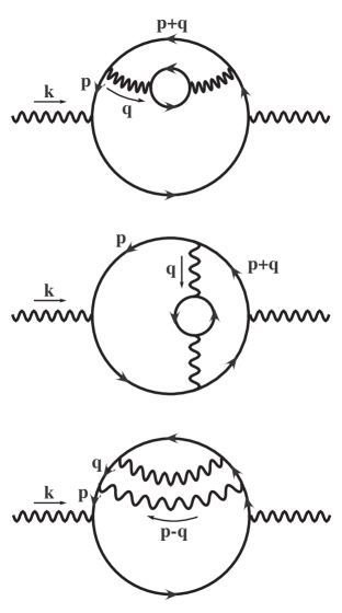
Figure 6: Three-loop diagrams for the photon polarization in the leading logarithmic approximation.

Origin of the leading logarithms

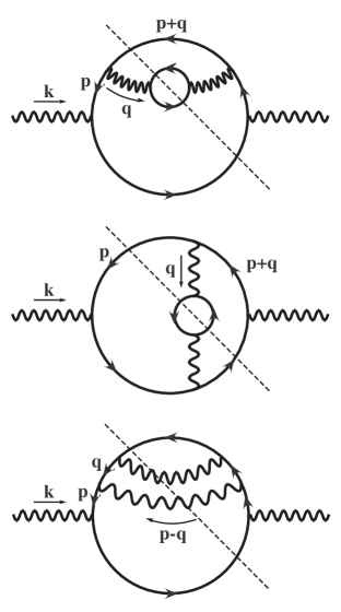
Figure 7: Cuts in the three-loop diagrams for the photon polarization in the leading logarithmic approximation that lead to the secular term. The dashed lines determine the cuts.

An important aspect gleaned from the above result is that the leading logarithmic correction can be extracted by using the perturbative spectral functions given by eq. (93) and by cutting off the integral over the transfer momentum $q$ with upper and lower cutoffs $q_{\mathrm{max}}\sim T$ and $q_{\mathrm{min}}\sim eT$, respectively. This simplification corresponds to computing the three-loop diagrams depicted in Fig. 6 with cutoff momentum integrals. The imaginary parts of the polarization that lead to the secular term and leading logarithmic contribution correspond to the cuts displayed in Fig. 7. The cut-diagrams with the photon self-energy correspond to Møller scattering $e^{\pm}\,e^{\pm}\rightarrow e^{\pm}\,e^{\pm}$, since the singular denominators that lead to secular terms arise from the products $\rho^{\pm}_{F}\;\rho^{\pm}_{F}$ and the photon spectral function below the light cone in the HTL approximation arises also from these type of products in the photon polarization bubble. The internal longitudinal (transverse) photon propagators with momentum $q$ contributes the factor $(q^{2})^{-2}$ [$(q^{2}_{0}-q^{2})^{-2}$] that leads to the logarithms. The cut-diagram with the fermion self-energy corresponds to Compton scattering $\gamma\,e^{\pm}\rightarrow\gamma\,e^{\pm}$ as well as pair annihilation and creation processes $e^{+}\,e^{-}\leftrightarrow\gamma+\gamma$, where the electrons, positrons and photons are all hard. The internal fermion propagators with momentum $q$ give rise the factor $(q_{0}\mp q)^{-2}$ that leads to the logarithms.

The diagrams that yield the leading logarithms in the coupling are formally corrections of $\mathcal{O}(e^{6})$ to the photon polarization. The logarithms arise from the free intermediate state propagators with momentum restricted by the upper and lower cutoffs $q_{\mathrm{max}}\sim T$ and $q_{\mathrm{\min}}\sim e~{}T$, respectively. Thus, only the polarization diagrams depicted in Fig. 7 with the simplified spectral functions eq. (93) and the upper and lower momentum cutoffs $q_{max}\sim T$, $q_{min}\sim e~{}T$ (or, alternatively, only the cut diagrams shown in Fig. 7 with restricted momentum transfer $eT\lesssim q\lesssim T$) contribute linear secular terms to leading logarithmic order. Such simplification in the leading logarithmic approximation has already been noticed in Ref. baym . In turn, this implies that both Debye screening for the longitudinal photon and dynamical screening by Landau damping for the transverse photon propagators are irrelevant to extract the leading logarithmic contribution and we can simply extract the leading secular terms to leading logarithmic accuracy by computing the three-loop corrections to the polarization with free vacuum photon propagators and upper and lower momentum cutoffs of order $T$ and $eT$, respectively. This observation will be important below where we establish the correspondence with the Boltzmann equation.

This analysis also allows to identify the diagrams in the perturbative expansion that yield the leading logarithmic contribution and the linear secular terms. To leading logarithmic order there are additional corrections to the polarization formally of $\mathcal{O}(e^{6})$, as depicted in Fig. 8. They correspond to a vertex correction to the fermion self-energy and a crossed ladder diagram. The calculation of these diagrams is very complicated and beyond the scope of this article. However, from the discussion above it is clear that these diagrams will feature a linear secular term but no logarithms of the coupling.

This above discussion highlights the origin of the leading logarithmic contributions and we can now argue firmly that the contribution from the diagram in Fig. 4(b) (or, equivalently, those depicted in Fig. 5) is subleading at leading logarithmic order. As argued after eq. (87), it is the term proportional to $1/\omega^{2}$ that can lead to secular terms. To leading order we can replace the HTL fermion spectral function ${}^{\ast}\!\rho_{+}(p_{0},p)$ in eq. (87) by that given in eq. (93). As a result, the contributions from the diagrams in Fig. 5 are of $\mathcal{O}(e^{8})$ and $\mathcal{O}(e^{10})$, respectively. Therefore, the soft-fermion contribution to the vertex is subleading in agreement with the conclusion of Ref. aarts .

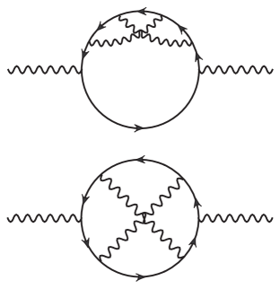
Figure 8: Three-loop photon polarization diagrams of $\mathcal{O}(e^{6})$ that feature a linear secular term but no logarithms in the coupling.

V Dynamical renormalization group and Boltzmann equation

In the previous sections we have extracted the corrections to the photon polarization that feature linear secular terms in time to leading logarithmic approximation. The next task is to sum the secular terms in the perturbative expansion by using the dynamical renormalization group approach introduced in Ref. boyanqed ; scalar . The dynamical renormalization group applies to the equation of motion of expectation values, either of the Heisenberg fields or of composite operators boyanqed ; scalar which lead to an initial value problem. Thus the first step is to obtain the corresponding equations of motion for $\mathcal{G}(t)$ or an alternative quantity from which it can be derived. In order to understand what are the equations of motion (and corresponding initial value problem) for $\mathcal{G}(t)$ (or a related quantity), we begin with equation eq. (28) which basically identifies $\mathcal{G}(t)$ with the time derivative of the expectation value of the current in the zero-momentum limit. Thus we now study the expectation value of the current to identify the proper equation of motion in order to implement the DRG resummation.

We begin the analysis by writing

$$\Psi(\mathbf{x}{},t{})=\sum_{\lambda}\int\frac{d^{3}p}{(2\pi)^{3}}\left[b_{\mathbf{p},\lambda}(t)\;u_{\mathbf{p},\lambda}\;e^{-i(pt-\mathbf{p}\cdot\mathbf{x}{})}+d^{\dagger}_{\mathbf{p},\lambda}(t)\;v_{\mathbf{p},\lambda}\;e^{i(pt-\mathbf{p}\cdot\mathbf{x}{})}\right]\;,$$ (97)

where $u$ and $v$ are the free massless Dirac spinors. The time evolution of the operators $b_{\mathbf{p},\lambda}(t)$ and $d_{\mathbf{p},\lambda}(t)$ is determined by the Heisenberg equations of motion. Here we have factored out the rapidly varying phases $e^{\mp ipt}$, therefore for momentum $p\sim T\gg m$ these operators vary slowly only due to the interaction. An important aspect of the gauge invariant formulation introduced earlier is that the operators $b$ and $d$ are manifestly gauge invariant, since the field operator $\Psi$ has been constructed to be manifestly gauge invariant.

Using the properties of the free massless Dirac spinors $u$ and $v$, we find that the zero momentum limit of the expectation value of the electromagnetic current is given by

$$J^{i}(t)=J^{i}_{c}(t)+J^{i}_{s}(t)\;,$$ (98)

with

$$J^{i}_{c}(t) = e\sum_{\lambda}\int\frac{d^{3}p}{(2\pi)^{3}}\;\hat{p}^{i}\;\Big{[}\langle b^{\dagger}_{\mathbf{p},\lambda}(t)\;b_{\mathbf{p},\lambda}(t)\rangle-\langle d_{-\mathbf{p},\lambda}(t)\;d^{\dagger}_{-\mathbf{p},\lambda}(t)\rangle\Big{]}\;,$$ (99)

$$J^{i}_{s}(t) = -ie\sum_{\lambda,\lambda^{\prime}}\int\frac{d^{3}p}{(2\pi)^{3}}\Big{[}\langle b^{\dagger}_{\mathbf{p},\lambda}(t)\;d^{\dagger}_{\mathbf{p},\lambda^{\prime}}(t)\rangle\;u^{\dagger}_{\mathbf{p},\lambda}\;(\mathbf{p}\times\!\bm{\Sigma})^{i}\;v_{-\mathbf{p},\lambda^{\prime}}\;e^{2ipt}\Big{]}+\mathrm{c.c.}\;,$$ (100)

where $\Sigma^{i}$ are the spin matrices. The term $\mathbf{J}_{c}(t)$ is the convection current and $\mathbf{J}_{s}(t)$ is the spin current. The convection current term is time independent in the free theory and is therefore varying slowly in the interacting theory, the time variation is solely due to the interactions. On the other hand, the spin current term mixes particles and antiparticles and oscillates very fast (even in free field theory), on time scales $p^{-1}\sim 1/T$. This term is responsible for the phenomenon of zitterbewegung associated with the mixture of positive and negative energy solutions in relativistic fermionic wave packets. Thus under the assumption that processes associated with photon exchange will not mix particles and antiparticles, namely that the exchanged photon momenta are $\ll T$, we can neglect the contribution from the spin current term since it oscillates very fast and will average out on time scales $\sim 1/T$.

Introducing the spatial Fourier transforms of the fermion fields

$$\Psi(\mathbf{x}{},t{})=\int\frac{d^{3}p}{(2\pi)^{3}}\;\Psi(\mathbf{p},t)\;e^{i\mathbf{p}\cdot\mathbf{x}{}}\;,\quad\Psi^{\dagger}(\mathbf{x}{},t{})=\int\frac{d^{3}p}{(2\pi)^{3}}\;\Psi^{\dagger}(\mathbf{p},t)\;e^{-i\mathbf{p}\cdot\mathbf{x}{}}\;,$$ (101)

we find the following expressions for the expectation values that enter in the convection current

$$\sum_{\lambda}\langle b^{\dagger}_{\mathbf{p},\lambda}(t)\;b_{\mathbf{p},\lambda}(t)\rangle=\langle\bar{\Psi}(\mathbf{p},t)\;\gamma_{-}(\widehat{\mathbf{p}})\;\Psi(\mathbf{p},t)\rangle\;,\quad\sum_{\lambda}\langle d_{-\mathbf{p},\lambda}(t)\;d^{\dagger}_{-\mathbf{p},\lambda}(t)\rangle=\langle\bar{\Psi}(\mathbf{p},t)\;\gamma_{+}(\widehat{\mathbf{p}})\;\Psi(\mathbf{p},t)\rangle\;.$$ (102)

These are identified as the contributions from positive and negative energy components to the convection current. Under the assumption that all the processes involved do not lead to a mixture of positive and negative energy components, the two contributions will not mix in any order of perturbation theory. This is manifest in the perturbative calculation of the previous section in that only products of spectral functions for particles or antiparticles enter in the secular terms. Thus the slowly varying part of the current at zero momentum is determined by the convection term and given by the expression

$$J^{i}_{c}(t)=e\int\frac{d^{3}p}{(2\pi)^{3}}\;\hat{p}^{i}\;\left[\langle\bar{\Psi}(\mathbf{p},t)\;\gamma_{-}(\widehat{\mathbf{p}})\;\Psi(\mathbf{p},t)\rangle-\langle\bar{\Psi}(\mathbf{p},t)\;\gamma_{+}(\widehat{\mathbf{p}})\;\Psi(\mathbf{p},t)\rangle\right]=e\int\frac{d^{3}p}{(2\pi)^{3}}\;\hat{p}^{i}\;\langle\bar{\Psi}(\mathbf{p},t)\;\bm{\gamma}\cdot\widehat{\mathbf{p}}\;\Psi(\mathbf{p},t)\rangle\;.$$ (103)

It proves convenient to introduce the spin-averaged expectation values of the number of particles and antiparticles as

$$f(\mathbf{p},t)=\frac{1}{2}\sum_{\lambda}\langle b^{\dagger}_{\mathbf{p},\lambda}(t)\;b_{\mathbf{p},\lambda}(t)\rangle\;,\quad\overline{f}(\mathbf{p},t)=\frac{1}{2}\sum_{\lambda}\langle d^{\dagger}_{\mathbf{p},\lambda}(t)\;d_{\mathbf{p},\lambda}(t)\rangle\;,$$ (104)

which as emphasized above are gauge invariant. In terms of these, the convection part of the current is given by

$$J^{i}_{c}(t)=2e\int\frac{d^{3}p}{(2\pi)^{3}}\,\hat{p}^{i}\left[f(\mathbf{p},t)+\overline{f}(-\mathbf{p},t)\right]\;,$$ (105)

which is the same form as that in kinetic theory, hence we call this the kinetic current. This analysis clearly highlights two important aspects: (i) The kinetic current is identified with the expectation value of the convection current in Dirac theory, this is the component that varies slowly on the time scale $1/T$, the contribution from the spin current averages out on time scales larger than $1/T$ provided there are no processes with transferred momenta $\sim 2T$ that can mix particles with antiparticles. (ii) The distribution functions $f$ and $\overline{f}$ are identified as the expectation values of the number operators for particles and antiparticles, respectively. Our gauge invariant formulation guarantees that these are indeed gauge invariant physical observables.

¿From now on we will refer to the current simply as the convection part and the discussion above clearly indicates that this is the kinetic current. Thus we can establish the following correspondence between the quantum field theory and the kinetic approach [see eq. (98)]:

$$J^{i}(t)=-ie\int\frac{d^{3}p}{(2\pi)^{3}}\;\hat{p}^{i}\;\mathrm{Tr}\left[\bm{\gamma}\cdot\widehat{\mathbf{p}}\;S^{<}(\mathbf{p};t,t)\right]\;,$$

$$\;f(\mathbf{p},t)=-\frac{i}{2}\mathrm{Tr}\left[\gamma_{-}(\widehat{\mathbf{p}})\;S^{<}(\mathbf{p};t,t)\right]\;,$$

$$\overline{f}(-\mathbf{p},t)=1+\frac{i}{2}\mathrm{Tr}\left[\gamma_{+}(\widehat{\mathbf{p}})\;S^{<}(\mathbf{p};t,t)\right]\;.$$ (106)

The correspondence given by eq. (106) makes manifest that the kinetic current is determined by the equal-time limit of the spatial Fourier transform of the full fermion propagator. The full fermion propagator is given by a Dyson sum

$$S=S_{0}+S_{0}\;\Sigma\;S_{0}+S_{0}\;\Sigma\;S_{0}\;\Sigma S_{0}+\cdots.$$ (107)

If an external electric field $\bm{\mathcal{E}}=-\dot{\bm{\mathcal{A}}_{T}}$ is present, then $S_{0}$ is the free propagator in the presence of the background gauge field $\bm{\mathcal{A}}_{T}$ but without corrections from interaction due to the fluctuating gauge fields, which are contained in the self-energy $\Sigma$. This observation for the kinetic current makes explicit that the collision term that enters the Boltzmann equation is determined by the fermion self-energy (see below).

Furthermore, at this stage we can make contact with the function $\mathcal{G}^{ij}(t)$ defined by the linear response relation eq. (28). For this purpose we define to linear order in the external electric field

$$f(\mathbf{p},t)=n_{F}(p)+\bm{\mathcal{E}}\cdot\widehat{\mathbf{p}}\;\Lambda(p,t)\;,\quad\overline{f}(-\mathbf{p},t)=n_{F}(p)+\bm{\mathcal{E}}\cdot\widehat{\mathbf{p}}\;\overline{\Lambda}(p,t)\;.$$ (108)

We therefore identify,

$$\mathcal{G}^{ij}(t)=-2e\int\frac{d^{3}p}{(2\pi)^{3}}\;\hat{p}^{i}\;\hat{p}^{j}\;\left[\dot{\Lambda}(p,t)+\dot{\overline{\Lambda}}(p,t)\right],$$ (109)

where the dot stands for derivative with respect to time. eq.(30) then leads to the following expression for the conductivity

$$\sigma=\frac{2e}{3}\int\frac{d^{3}p}{(2\pi)^{3}}\,\left[{\Lambda}(p,t=\infty)+{\overline{\Lambda}}(p,t=\infty)\right],$$ (110)

where we have used the initial condition ${\Lambda}(p,t=0)={\overline{\Lambda}}(p,t=0)=0$.

We now derive the Boltzmann equation for the distribution functions $f$ and $\overline{f}$ in the presence of the background gauge field by implementing the dynamical renormalization group. We first calculate the time derivative of these distribution functions to linear order in the background gauge field as in Sec. II.2 and extract the positive and negative energy components of the coefficient of $\hat{p}^{i}$ from the HTL photon polarization. As discussed in Sec. III.1 the polarization for small external frequency and momentum only receives contributions from the products of fermion spectral functions of the form $\rho_{+}\;\rho_{+}$ and $\rho_{-}\;\rho_{-}$, corresponding to the positive and energy fermion mass shells respectively. This explicitly shows that there is no mixing between positive and negative energy components in the small transferred momentum limit, thus justifying the neglect of the spin current contribution.

We assume that at a given time $t_{0}$ the initial density matrix is diagonal in the number basis and that the number operators for fermion and antifermion have respective expectation values $f(\mathbf{p},t_{0})$ and $\overline{f}(\mathbf{p},t_{0})$ as given by eq. (104). This choice of the initial density matrix entails that the fermion propagators have the free field form as given in Appendix B but in terms of the nonequilibrium distributions $f(\mathbf{p},t_{0})$ and $\overline{f}(\mathbf{p},t_{0})$ at time $t_{0}$ (see also Ref. boyanqed ). From the results of Sec. III.1 we find to lowest order in the background field and leaving the calculation of the collision terms (arising from the interaction with the photon fields, namely the self-energy corrections) for the moment, that the time derivative of the distribution functions are determined by the HTL photon polarization. Using the nonequilibrium fermion propagators given in Appendix B, we find

$$\frac{\partial}{\partial t}f(\mathbf{p},t)=-e\,\bm{\mathcal{E}}\cdot\!\bm{\nabla}_{\mathbf{p}}f(\mathbf{p},t_{0})+\mbox{collision~{}terms}\;,\quad\frac{\partial}{\partial t}\overline{f}(-\mathbf{p},t)=-e\,\bm{\mathcal{E}}\cdot\!\bm{\nabla}_{\mathbf{p}}\overline{f}(-\mathbf{p},t_{0})+\mbox{collision~{}terms}\;.$$ (111)

The next step is to obtain the contribution to the time derivative of the distribution functions from the interaction, namely the collision term. From the definition of the distribution functions eq. (104), it follows that their time derivatives are completely determined by the Heisenberg equations for the fermion fields, namely,

$$\frac{\partial}{\partial t}\Psi(\mathbf{p},t)=-i\,\bm{\alpha}\cdot\mathbf{p}\;\Psi(\mathbf{p},t)+ie\int\frac{d^{3}q}{(2\pi)^{3}}\left[\bm{\alpha}\cdot\mathbf{A}_{T}(\mathbf{q},t)-A^{0}(\mathbf{q},t)\right]\Psi(\mathbf{p}-\mathbf{q},t)\;.$$ (112)

Taking the time derivative of the distribution functions and using eq. (112), we find that the collision term for $f(\mathbf{p},t)$ is given by boyanqed

$$\frac{\partial f(\mathbf{p},t)}{\partial t}\bigg{|}_{\mathrm{coll}} = \frac{ie}{2}\int\frac{d^{3}q}{(2\pi)^{3}}\big{[}\big{\langle}\bar{\Psi}^{-}(\mathbf{p}+\mathbf{q},t)A^{0,-}(\mathbf{q},t)\gamma_{-}(\widehat{\mathbf{p}})\Psi^{+}(\mathbf{p},t)\big{\rangle}$$ (113)

$$-\big{\langle}\bar{\Psi}^{-}(\mathbf{p}+\mathbf{q},t)\bm{\gamma}\cdot\mathbf{A}^{-}_{T}(\mathbf{q},t)\gamma^{0}\gamma_{-}(\widehat{\mathbf{p}})\Psi^{+}(\mathbf{p},t)\big{\rangle}\big{]}+\mathrm{c.c.}\;,$$

where the superscripts ‘$\pm$’ refer to fields in the forward and backward branches in closed-time-path formalism, respectively (see  boyanqed for details) . The collision term for $\overline{f}(-\mathbf{p},t)$ has a similar expression but with $\gamma_{-}(\widehat{\mathbf{p}})\to-\gamma_{+}(\widehat{\mathbf{p}})$. The expectation values in these expressions are in an initial density matrix and can be systematically computed in perturbation theory. In order to compute the time derivative of the distribution function in eq. (113) we now follow the procedure outlined in Sec. IV B in Ref. boyanqed .

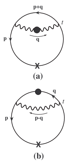
Figure 9: Diagrams corresponding to the collision term $\partial f(\mathbf{p},t)/\partial t|_{\mathrm{coll}}$ up to one-loop order: (a) the soft-photon contribution and (b) the soft-fermion contribution. The solid line denotes the free fermion propagator in the presence of the background gauge field. The heavy cross in the fermion line represents the insertion of $\gamma^{0}\gamma_{-}$ at the time $t$.

Up to one-loop order, as depicted in Fig. 9, the collision term receives contributions from soft internal photon and soft internal fermion

$$\frac{\partial f(\mathbf{p},t)}{\partial t}\bigg{|}_{\mathrm{coll}} = C[f(.,t_{0}),\overline{f}(.,t_{0}),t-t_{0}]\equiv C^{\mathrm{sp}}[f(.,t_{0}),\overline{f}(.,t_{0}),t-t_{0}]+C^{\mathrm{sf}}[f(.,t_{0}),\overline{f}(.,t_{0}),t-t_{0}]\;.$$ (114)

Following the steps detailed in Ref. scalar ; boyanqed with the propagators given in Appendix B, we find that the collision term can be written in an illuminating form which displays the familiar gain minus loss form as

$$C[f(.,t_{0}),\overline{f}(.,t_{0});t-t_{0}]=2\int^{+\infty}_{-\infty}dp_{0}\;\frac{\sin\left[(p-p_{0})(t-t_{0})\right]}{\pi(p-p_{0})}\left\{\left[1-f(\mathbf{p},t_{0})\right]\;\Sigma_{>}(p_{0},p)-f(\mathbf{p},t_{0})\Sigma_{<}(p_{0},p)\right\}\;,$$ (115)

where

$$\Sigma_{>}(p_{0},p)=\Sigma^{\mathrm{sp}}_{>}(p_{0},p)+\Sigma^{\mathrm{sf}}_{>}(p_{0},p)\;,\quad\Sigma_{<}(p_{0},p)=\Sigma^{\mathrm{sp}}_{<}(p_{0},p)+\Sigma^{\mathrm{sf}}_{<}(p_{0},p)\;,$$ (116)

with the following self-energy components

$$\Sigma^{\mathrm{sp}}_{>}(p_{0},p) = e^{2}\pi\int\frac{d^{3}q}{(2\pi)^{3}}\int^{+\infty}_{-\infty}dq_{0}\big{\{}\big{[}K^{+}_{1}(\mathbf{p},\mathbf{q})\;{}^{\ast}\!\rho_{L}(q_{0},q)+K^{+}_{2}(\mathbf{p},\mathbf{q})\;{}^{\ast}\!\rho_{T}(q_{0},q)\big{]}$$

$$\times\,f(\mathbf{p}+\mathbf{q},t_{0})\;n_{B}(q_{0})\;\delta(p_{0}-q_{0}-|\mathbf{p}+\mathbf{q}|)+\,\big{[}K^{-}_{1}(\mathbf{p},\mathbf{q})\;{}^{\ast}\!\rho_{L}(q_{0},q)+K^{-}_{2}(\mathbf{p},\mathbf{q})\;{}^{\ast}\!\rho_{T}(q_{0},q)\big{]}$$

$$\times\,[1-\overline{f}(-\mathbf{p}-\mathbf{q},t_{0})]\;n_{B}(q_{0})\;\delta(p_{0}-q_{0}+|\mathbf{p}+\mathbf{q}|)\big{\}}\;,$$

$$\Sigma^{\mathrm{sp}}_{<}(p_{0},p) = e^{2}\pi\int\frac{d^{3}q}{(2\pi)^{3}}\int^{+\infty}_{-\infty}dq_{0}\;\big{\{}\big{[}K^{+}_{1}(\mathbf{p},\mathbf{q})\;{}^{\ast}\!\rho_{L}(q_{0},q)+K^{+}_{2}(\mathbf{p},\mathbf{q})\;{}^{\ast}\!\rho_{T}(q_{0},q)\big{]}$$ (117)

$$\times\,[1-f(\mathbf{p}+\mathbf{q},t_{0})][1+n_{B}(q_{0})]\;\delta(p_{0}-q_{0}-|\mathbf{p}+\mathbf{q}|)+\,\big{[}K^{-}_{1}(\mathbf{p},\mathbf{q})\;{}^{\ast}\!\rho_{L}(q_{0},q)+K^{-}_{2}(\mathbf{p},\mathbf{q})\;{}^{\ast}\!\rho_{T}(q_{0},q)\big{]}$$

$$\times\,\overline{f}(-\mathbf{p}-\mathbf{q},t_{0})\;[1+n_{B}(q_{0})]\;\delta(p_{0}-q_{0}+|\mathbf{p}+\mathbf{q}|)\big{\}}\;,$$

and

$$\Sigma^{\mathrm{sf}}_{>}(p_{0},p) = \pi e^{2}\int\frac{d^{3}q}{(2\pi)^{3}}\frac{1}{2|\mathbf{p}-\mathbf{q}|}\int^{+\infty}_{-\infty}dq_{0}\;\big{\{}\big{[}K^{+}_{3}(\mathbf{p},\mathbf{q})\;{}^{\ast}\!\rho_{+}(q_{0},q)+K^{-}_{3}(\mathbf{p},\mathbf{q})\;{}^{\ast}\!\rho_{-}(q_{0},q)\big{]}$$

$$\times\,n_{F}(q_{0})\;n_{B}(|\mathbf{p}-\mathbf{q}|)\;\delta(p_{0}-q_{0}-|\mathbf{p}-\mathbf{q}|)+\,\big{[}K^{-}_{3}(\mathbf{p},\mathbf{q})\;{}^{\ast}\!\rho_{+}(q_{0},q)+K^{+}_{3}(\mathbf{p},\mathbf{q})\;{}^{\ast}\!\rho_{-}(q_{0},q)\big{]}$$

$$\times\,[1-n_{F}(q_{0})][1+n_{B}(|\mathbf{p}-\mathbf{q}|)]\;\delta(p_{0}+q_{0}+|\mathbf{p}-\mathbf{q}|)\big{\}}\;,$$

$$\Sigma^{\mathrm{sf}}_{<}(p_{0},p) = \pi e^{2}\int\frac{d^{3}q}{(2\pi)^{3}}\frac{1}{2|\mathbf{p}-\mathbf{q}|}\int^{+\infty}_{-\infty}dq_{0}\;\big{\{}\big{[}K^{+}_{3}(\mathbf{p},\mathbf{q})\;{}^{\ast}\!\rho_{+}(q_{0},q)+K^{-}_{3}(\mathbf{p},\mathbf{q})\;{}^{\ast}\!\rho_{-}(q_{0},q)\big{]}$$ (118)

$$\times\,[1-n_{F}(q_{0})][1+n_{B}(|\mathbf{p}-\mathbf{q}|)]\;\delta(p_{0}-q_{0}-|\mathbf{p}-\mathbf{q}|)$$

$$+\,\big{[}K^{-}_{3}(\mathbf{p},\mathbf{q})\;{}^{\ast}\!\rho_{+}(q_{0},q)+K^{+}_{3}(\mathbf{p},\mathbf{q}){}^{\ast}\!\rho_{-}(q_{0},q)\big{]}\;n_{F}(q_{0})\;n_{B}(|\mathbf{p}-\mathbf{q}|)\;\delta(p_{0}+q_{0}+|\mathbf{p}-\mathbf{q}|)\big{\}}\;.$$

For antiparticles we find that

$$\frac{\partial\overline{f}(\mathbf{p},t)}{\partial t}\bigg{|}_{\mathrm{coll}}=\overline{C}[f(.,t_{0}),\overline{f}(.,t_{0});t-t_{0}]\;,$$ (119)

where

$$\overline{C}[f(\mathbf{p},t_{0}),\overline{f}(-\mathbf{q},t_{0});t-t_{0}]=C[\overline{f}(-\mathbf{p},t_{0}),f(\mathbf{q},t_{0});t-t_{0}]\;,$$ (120)

which entails that $f(\mathbf{p},t)$ and $\overline{f}(-\mathbf{p},t)$ satisfy the same evolution equations. Since the evolution equation for antiparticles (with momentum $-\mathbf{p}$) is identical to that for particles (with momentum $\mathbf{p}$), we now focus solely on the particle distribution function, the steps can be repeated straightforwardly for the distribution of antiparticles.

V.1 DRG resummation of the secular terms

Combining eq. (111) with the collision term obtained above we find

$$\frac{\partial}{\partial t}f(\mathbf{p},t)=-e\,\bm{\mathcal{E}}\cdot\!\bm{\nabla}_{\mathbf{p}}f(\mathbf{p},t_{0})+C[f(.,t_{0}),\overline{f}(.,t_{0});t-t_{0}].$$ (121)

Notice that the right-hand side depends only on time through the sine functions in the collision term, and the distribution functions $f(\mathbf{p},t_{0})$ and $f(-\mathbf{p},t_{0})$ are fixed at the initial time [see eq. (115)]. Thus the evolution equation can be integrated to yield

$$f(\mathbf{p},t)=f(\mathbf{p},t_{0})-e\;\bm{\mathcal{E}}\cdot\!\bm{\nabla}_{\mathbf{p}}f(\mathbf{p},t_{0})\;(t-t_{0})+\int^{t}_{t_{0}}C[f(.,t_{0}),\overline{f}(.,t_{0});t^{\prime}-t_{0}]\;dt^{\prime}\;.$$ (122)

The last term gives upon integration on time,

$$\int^{t}_{t_{0}}C[f(.,t_{0}),\overline{f}(.,t_{0});t^{\prime}-t_{0}]\;dt^{\prime}=\int^{+\infty}_{-\infty}dp_{0}\;\frac{1-\cos[(p-p_{0})(t-t_{0})]}{\pi(p-p_{0})^{2}}\;\mathcal{K}(f(.,t_{0}),\overline{f}(.,t_{0});p_{0},p)\;,$$ (123)

with

$$\mathcal{K}(f(.,t_{0}),\overline{f}(.,t_{0});p_{0},p) = 2\left\{\left[1-f(\mathbf{p},t_{0})\right]\;\Sigma_{>}(p_{0},p)-f(\mathbf{p},t_{0})\Sigma_{<}(p_{0},p)\right\}\;.$$ (124)

In general the time integral of the collision term will feature secular terms, whose time dependence is determined by the behavior of the term that multiplies the cosine near the resonance $p=p_{0}$. For example, if the coefficient of the cosine term $\mathcal{K}(f(.,t_{0}),\overline{f}(.,t_{0});p_{0},p)$ is finite and does not feature any singularity as $p-p_{0}\to 0$ then we can use the long-time asymptotic expression scalar

$$\frac{1-\cos[(p-p_{0})(t-t_{0})]}{\pi(p-p_{0})^{2}}\to(t-t_{0})\;\delta(p-p_{0})$$ (125)

to extract the secular term, which in this case is linear in time as is the case in the usual Fermi’s Golden rule. However, if $\mathcal{K}(f(.,t_{0}),\overline{f}(.,t_{0});p_{0},p)$ either vanishes or features singularities near the resonance $p=p_{0}$ then one must be more careful in extracting the secular term. Such is the case with the anomalous logarithms that will emerge in the relaxation time approximation (see below). Whatever the form of these secular terms, their main feature is that they grow in time and invalidate the perturbative expansion, therefore they must be resummed. This resummation scheme in real time is the goal of the dynamical renormalization group program boyanqed ; scalar .

Just as the usual renormalization group absorbs the divergences into a renormalization of couplings at an arbitrary momentum scale, the dynamical renormalization group absorbs the secular terms into a finite renormalization of the distribution function at an arbitrary time scale $\tau$. Let us define

$$f(\mathbf{p},t_{0})=f(\mathbf{p},\tau)\;\mathcal{Z}(\mathbf{p},\tau,t_{0}),$$ (126)

where the renormalization constant $\mathcal{Z}$ will be chosen in an expansion in $\mathcal{E}$ and the coupling that enters in the collision term to cancel the secular terms in eq. (122) at the time $t=\tau$. Choosing to lowest order

$$\mathcal{Z}(\mathbf{p},\tau,t_{0})=1+\frac{e\,\bm{\mathcal{E}}\cdot\!\bm{\nabla}_{\mathbf{p}}f(\mathbf{p},\tau)}{f(\mathbf{p},\tau)}(\tau-t_{0})-\int^{\tau}_{t_{0}}\frac{C_{s}[f(.,\tau),\overline{f}(.,\tau);t^{\prime}-t_{0}]}{f(\mathbf{p},\tau)}\;dt^{\prime}+\mathcal{O}(\mathcal{E}^{2},C^{2}_{s},\mathcal{E}\;C_{s})\;,$$ (127)

where $C_{s}$ denotes the part of the collision term that leads to secular terms. Then to lowest order in the external background field and in the strength of the collision term we find

$$f(\mathbf{p},t)=f(\mathbf{p},\tau)-e\,\bm{\mathcal{E}}\cdot\!\bm{\nabla}_{\mathbf{p}}f(\mathbf{p},\tau)(t-\tau)-\int^{\tau}_{t}C_{s}[f(.,\tau),\overline{f}(.,\tau);t^{\prime}-t_{0}]\;dt^{\prime}+\mathcal{O}(\mathcal{E}^{2},C^{2}_{s},\mathcal{E}\;C_{s})+\mbox{non~{}secular~{}terms}\;,$$ (128)

Choosing the arbitrary scale $\tau$ near $t$, the perturbative expansion is now valid in a neighborhood of $t=\tau$ by renormalizing the distribution function.

However, the distribution function $f(\mathbf{p},t)$ cannot depend on the arbitrary time scale $\tau$, namely $df(\mathbf{p},t)/d\tau=0$ leads to the dynamical renormalization group equation to this order (after setting $\tau=t$)

$$\frac{\partial}{\partial t}f(\mathbf{p},t)+e\,\bm{\mathcal{E}}\cdot\!\bm{\nabla}_{\mathbf{p}}f(\mathbf{p},t)=C_{s}[f(.,t),\overline{f}(.,t);t]\;.$$ (129)

This dynamical renormalization group equation is recognized as the Boltzmann equation, where the collision term is the part of the original one that leads to secular terms. (See Ref. scalar for the scalar theory). Thus in order to write down the Boltzmann equation we must first work out $C_{s}$. As we shall see below in sec. V C, when $\mathcal{K}(f(.,t_{0}),\overline{f}(.,t_{0});p_{0},p)$ is regular at $p_{0}=p$, we simply find

$$C_{s}[f(.,t),\overline{f}(.,t);t]=\mathcal{K}(f(.,t),\overline{f}(.,t);p,p)\;.$$

V.2 Relaxation time approximation

In the relaxation time approximation only the particles with momentum $\mathbf{p}$ and the antiparticles with momentum $-\mathbf{p}$ are slightly distorted out of equilibrium, while particles and antiparticles with all other momenta are assumed to be in equilibrium. Hence, we write the particle distribution as

$$f(\mathbf{p},t_{0})=n_{F}(p)+\delta f(\mathbf{p},t_{0})\;,\quad f(\mathbf{p}+\mathbf{q},t_{0})=n_{F}(|\mathbf{p}+\mathbf{q}|)\;\;\mathrm{for}\;\;\mathbf{q}\neq 0\;,$$ (130)

and similarly for antiparticle distributions. With the above distributions the collision term given by eq. (115) simplifies to

$$C[f(.,t_{0}),\overline{f}(.,t_{0});t-t_{0}]=-2\;\delta f(\mathbf{p},t_{0})\int^{+\infty}_{-\infty}dp_{0}\;\Sigma_{+}(p_{0},p)\;\frac{\sin\left[(p-p_{0})(t-t_{0})\right]}{\pi(p-p_{0})}\;,$$ (131)

where we have used the fact that when evaluated with the equilibrium distribution ($n_{F}(p)$), $\mathcal{K}(n_{F}(.),n_{F}(.);p_{0},p)$ vanishes by virtue of detailed balance and $\Sigma_{>}(p_{0},p)+\Sigma_{<}(p_{0},p)=\Sigma_{+}(p_{0},p)$ with $\Sigma_{+}(p_{0},p)$ given by eq. (41).

As discussed in Sec. III.3, the self-energy $\Sigma_{+}(p_{0},p)$ near the fermion mass shell is dominated by the ultrasoft photon exchange that leads to anomalous damping. Using eq. (46) and the results quoted in Refs. boyanqed ; scalar , the time integral in eq. (122) to linear order in the external electric field and the departure of equilibrium (considered to be of the same order as the external electric field) is given by

$$\delta f(\mathbf{p},t)=\delta f(\mathbf{p},t_{0})-e\,\bm{\mathcal{E}}\cdot\!\bm{\nabla}_{\mathbf{p}}n_{F}(p)(t-t_{0})-2\alpha T\,(t-t_{0})\,\ln\left[(t-t_{0})\omega_{D}\right]\,\delta f(\mathbf{p},t_{0})+\mathrm{subleading}\;.$$ (132)

This expression clearly displays the anomalous logarithms as secular terms found previously in the perturbative expression eq. (73).

Following the steps described above by introducing the renormalization constant $\mathcal{Z}(\mathbf{p},\tau,t_{0})$:

$$\delta f(\mathbf{p},t_{0})=\mathcal{Z}(\mathbf{p},\tau,t_{0})\;\delta f(\mathbf{p},\tau)\;,$$ (133)

with

$$\mathcal{Z}(\mathbf{p},\tau,t_{0})=1+e\,\bm{\mathcal{E}}\cdot\!\bm{\nabla}_{\mathbf{p}}n_{F}(p)(\tau-t_{0})+2\alpha T\,(\tau-t_{0})\,\ln\left[\omega_{D}(\tau-t_{0})\right]+{\cal O}(\mathcal{E}^{2},e^{3})\;,$$ (134)

we are led to the following DRG equation

$$\frac{\partial}{\partial t}\delta f(\mathbf{p},t)+e\,\bm{\mathcal{E}}\cdot\!\bm{\nabla}_{\mathbf{p}}n_{F}(p)=-2\;\Gamma(t)\;\delta f(\mathbf{p},t)\;,$$ (135)

with $\Gamma(t)$ the time dependent relaxation rate, which in the leading logarithmic approximation is given by (for $t\gg t_{0}$)

$$\Gamma(t)=\alpha\;T\left[\ln(\omega_{D}t)+1\right]\;.$$ (136)

The equation for $\delta\overline{f}(-\mathbf{p},t)$ is the same as that above for particles. The DRG equation (135) is the Boltzmann equation in the relaxation time approximation.

If $\Gamma$ were a constant the solution to the above equation would be

$$\delta f(\mathbf{p},t)=-e\,\bm{\mathcal{E}}\cdot\!\bm{\nabla}_{\mathbf{p}}\;n_{F}(p)\;\frac{1-e^{-2\Gamma t}}{2\Gamma}\;.$$ (137)

Using the relations given by eqs. (108)-(109) with this solution we would then find

$$\mathcal{G}^{ij}(t)=-{4e^{2}}\int\frac{d^{3}p}{(2\pi)^{3}}\;\frac{dn_{F}(p)}{dp}\;\hat{p}^{i}\;\hat{p}^{j}\;e^{-2\Gamma t}=\delta_{ij}\;\frac{e^{2}\;T^{2}}{9}\;e^{-2\Gamma t}\;.$$ (138)

This is exactly the result that we would find if we considered the fermion propagator obtained from the Dyson resummation with a constant width, as discussed in Sec. IV.2. Thus we see that in the case in which the width is constant, the DRG resummation in the relaxation time approximation is equivalent to the Dyson resummation of the fermion propagator boyanqed ; scalar . The result (138) leads to a steady-state, drift current at long times given by

$$J^{i}=-\frac{4e^{2}}{2\Gamma}\int\frac{d^{3}p}{(2\pi)^{3}}\;\hat{p}^{i}\;\bm{\mathcal{E}}\cdot\!\bm{\nabla}_{\mathbf{p}}n_{F}(p)=\frac{e^{2}T^{2}}{18\,\Gamma}\;\mathcal{E}^{i}\;,$$ (139)

and to the electrical conductivity

$$\sigma=\frac{e^{2}T^{2}}{18\,\Gamma}\;,$$ (140)

which is in complete agreement with that of the analysis of Sec. IV.2 for constant $\Gamma$.

However, for $\Gamma(t)$ given by eq. (136) the dynamical renormalization group equation (135) leads to a very different picture. The solution of eq. (135) with eq. (136) is given by

$$\delta f(\mathbf{p},t)=-e\,\bm{\mathcal{E}}\cdot\!\bm{\nabla}_{\mathbf{p}}\;n_{F}(p)\;e^{-2\alpha Tt\ln(\omega_{D}t)}\int^{t}_{0}\;e^{2\alpha Tt^{\prime}\ln(\omega_{D}t^{\prime})}\;dt^{\prime}\;,$$ (141)

where we have assumed that the electric field was switched-on at $t=0$ and that $\delta f(\mathbf{p},t=0)=0$. Taking the time derivative of this expression, using the identifications eqs. (108)-(109) and that the Boltzmann equation for antiparticles (with momentum $-\mathbf{p}$) is the same as that for particles (with momentum $\mathbf{p}$), we find to $\mathcal{O}(\alpha)$

$$\mathcal{G}^{ij}(t)=4e^{2}\int\frac{d^{3}p}{(2\pi)^{3}}\frac{dn_{F}(p)}{dp}\;\hat{p}^{i}\;\hat{p}^{j}\;\left[1-2\alpha Tt\ln(\omega_{D}t)\right]=-\delta_{ij}\;\frac{e^{2}T^{2}}{9}\;\left[1-2\alpha Tt\ln(\omega_{D}t)\right]\;,$$ (142)

namely, the solution of the Boltzmann equation in the relaxation time approximation reproduces the leading secular term to $\mathcal{O}(\alpha)$ found in the perturbative expansion given by eq. (74).

Thus we reach an important result of this study: the relaxation time approximation in the Boltzmann equation is equivalent to only considering self-energy corrections to the internal fermion propagators in the photon polarization. This is a reassuring result and establishes a direct link between the perturbative expansion of self-energy corrections to the photon polarization and the Boltzmann equation in the relaxation time approximation.

Of course, these secular terms are an artifact of the approximation, the full solution given by eq. (141) is bound at all times. Its asymptotic long time behavior can be found as follows. First it is convenient to split the time integral in eq. (141) as $\int^{t}_{0}dt^{\prime}=\int^{1/\omega_{D}}_{0}dt^{\prime}+\int^{t}_{1/\omega_{D}}dt^{\prime}$. In the first integral $t^{\prime}\ln(\omega_{D}t^{\prime})<0$ hence we can replace $e^{2\alpha Tt\ln(\omega_{D}t)}\sim 1$, leading to an exponentially small contribution at asymptotically long time. The second integral can be computed by successive integration by parts which lead to the asymptotic expansion,

$$\delta f(\mathbf{p},t)=-\frac{e\,\bm{\mathcal{E}}\cdot\!\bm{\nabla}_{\mathbf{p}}n_{F}(p)}{2\alpha T\ln(\omega_{D}t)}\left[1+\frac{1}{2\alpha Tt\ln^{2}(\omega_{D}t)}+\cdots\right]\;,$$ (143)

namely the drift current vanishes asymptotically, hence the logarithmic anomalous damping leads to a vanishing electrical conductivity. The main result of this analysis is that while a constant damping rate $\Gamma$ would lead to a finite conductivity given by eq. (140), an anomalous logarithmic time dependence of the damping rate leads to a vanishing electrical conductivity in the asymptotic, long-time limit.

Again we highlight that the result given by eq. (143) is a consequence of the relaxation time approximation which is equivalent to keeping only self-energy corrections. This result does not apply to the hot QED plasma because the vertex corrections introduce the cancellation analyzed in the previous section. The correct expression is given below by eqs. (155) and (174). We derived here eq. (143) to show what would be the solution if the relation time approximation were valid, which is not the case here.

V.3 Full and linearized Boltzmann equation

The above discussion on the relaxation time approximation highlights that this approximation is equivalent to considering only the self-energy corrections to the photon polarization. This conclusion is based on the equivalence of the secular terms between the perturbative result (74) and the lowest order in $\alpha$ term in the exact solution of the Boltzmann equation in the relaxation time approximation (142). The anomalous logarithms in time are a consequence of ultrasoft photon exchange leading to the threshold infrared divergence.

Just as in the perturbative case we expect that the cancellation of infrared divergences between self-energy and vertex corrections will also be manifest in the Boltzmann equation. Thus, we assume for a moment, and will be confirmed below, that the coefficient of the cosine term $\mathcal{K}(f(.,t_{0}),\overline{f}(.,t_{0});p_{0},p)$ in eq. (123) is non-singular and finite at $p_{0}=p$ and use the result eq. (125) to extract the asymptotic long time limit. In this case the secular term is linear in time, and we recognize that the collision term that enters in the Boltzmann equation (129) is given by

$$C_{s}[f(.,t),\overline{f}(.,t)]=C^{\mathrm{sp}}_{s}[f(.,t),\overline{f}(.,t)]+C^{\mathrm{sf}}_{s}[f(.,t),\overline{f}(.,t)]\;,$$ (144)

where

$$C^{\mathrm{sp}}_{s}[f(.,t),\overline{f}(.,t)] = 2\pi e^{2}\int\frac{d^{3}q}{(2\pi)^{3}}\int^{+\infty}_{-\infty}dq_{0}\big{\{}\big{[}K^{+}_{1}(\mathbf{p},\mathbf{q})\;{}^{\ast}\!\rho_{L}(q_{0},q)+K^{+}_{2}(\mathbf{p},\mathbf{q})\;{}^{\ast}\!\rho_{T}(q_{0},q)\big{]}\;\delta(p-q_{0}-|\mathbf{p}+\mathbf{q}|)$$ (145)

$$\times\big{[}[1-f(\mathbf{p},t)]\;f(\mathbf{p}+\mathbf{q},t)\;n_{B}(q_{0})-f(\mathbf{p},t)[1-f(\mathbf{p}+\mathbf{q},t)]\;[1+n_{B}(q_{0})]\big{]}$$

$$+\big{[}K^{-}_{1}(\mathbf{p},\mathbf{q})\;{}^{\ast}\!\rho_{L}(q_{0},q)+K^{-}_{2}(\mathbf{p},\mathbf{q})\;{}^{\ast}\!\rho_{T}(q_{0},q)\big{]}\;\delta(p-q_{0}+|\mathbf{p}+\mathbf{q}|)$$

$$\times\big{[}[1-f(\mathbf{p},t)]\;[1-\overline{f}(-\mathbf{p}-\mathbf{q},t)]n_{B}(q_{0})-f(\mathbf{p},t)\overline{f}(-\mathbf{p}-\mathbf{q},t)[1+n_{B}(q_{0})]\big{]}\big{\}}\;,$$

$$C^{\mathrm{sf}}_{s}[f(.,t),\overline{f}(.,t)] = \pi e^{2}\int\frac{d^{3}q}{(2\pi)^{3}}\frac{1}{|\mathbf{p}-\mathbf{q}|}\int^{+\infty}_{-\infty}dq_{0}\big{\{}\big{[}K^{+}_{3}(\mathbf{p},\mathbf{q})\;{}^{\ast}\!\rho_{+}(q_{0},q)+K^{+}_{3}(\mathbf{p},\mathbf{q})\;{}^{\ast}\!\rho_{-}(q_{0},q)\big{]}\;\delta(p-q_{0}-|\mathbf{p}-\mathbf{q}|)$$ (146)

$$\times\big{[}[1-f(\mathbf{p},t)]\;n_{F}(q_{0})\;n_{B}(|\mathbf{p}-\mathbf{q}|)-f(\mathbf{p},t)\;[1-n_{F}(q_{0})]\;[1+n_{B}(|\mathbf{p}-\mathbf{q}|)]\big{]}+$$

$$+\big{[}K^{-}_{3}(\mathbf{p},\mathbf{q})\;{}^{\ast}\!\rho_{+}(q_{0},q)+K^{-}_{3}(\mathbf{p},\mathbf{q})\;{}^{\ast}\!\rho_{-}(q_{0},q)\big{]}\;\delta(p+q_{0}+|\mathbf{p}-\mathbf{q}|)$$

$$\times\big{[}[1-f(\mathbf{p},t)]\;[1-n_{F}(q_{0})]\;[1+n_{B}(|\mathbf{p}-\mathbf{q}|)]-f(\mathbf{p},t)\;n_{F}(q_{0})\;n_{B}(|\mathbf{p}-\mathbf{q}|)\big{]}\big{\}}\;.$$

The reason that in the soft-fermion contribution $C^{\mathrm{sf}}_{s}$ there appear the free fermion distribution functions $n_{F}(q_{0})$ and not $f$ is a consequence of the fact that the HTL correction to the vertex does not lead to secular terms to lowest order as discussed above and analyzed in detail in Ref. aarts . This will become clear below when we identify self-energy and vertex contributions in the collision kernel of the Boltzmann equation and we compare the perturbative solution of the Boltzmann equation with the perturbative expansion of the function $\mathcal{G}(t)$ studied in the previous sections.

We notice that the delta functions $\delta(p-q_{0}+|\mathbf{p}+\mathbf{q}|)$ in eq. (145), which multiplies terms that mix particles ($f$) with antiparticles ($\overline{f}$), and $\delta(p+q_{0}+|\mathbf{p}+\mathbf{q}|)$ in eq. (146) can only be satisfied if $q_{0}\sim T$ since $p\sim T$ and $q\sim eT$. However, in obtaining the kinetic current we have neglected precisely these type of processes which are responsible for very fast oscillations on time scales $\sim\mathcal{O}(1/T)$ [see discussion after eqs. (99) and (100)].

To be consistent with the kinetic description, we must consider only processes in which the transfer of energy and momentum is $q_{0}$, $q\ll T$ and hence neglect the second terms in eqs. (145) and (146). Therefore, the correct Boltzmann equation to this order is given by

$$\frac{\partial}{\partial t}f(\mathbf{p},t)+e\,\bm{\mathcal{E}}\cdot\!\bm{\nabla}_{\mathbf{p}}f(\mathbf{p},t) = 2\pi e^{2}\int\frac{d^{3}q}{(2\pi)^{3}}\int^{+\infty}_{-\infty}dq_{0}\bigg{\{}\big{[}K^{+}_{1}(\mathbf{p},\mathbf{q})\;{}^{\ast}\!\rho_{L}(q_{0},q)+K^{+}_{2}(\mathbf{p},\mathbf{q})\;{}^{\ast}\!\rho_{T}(q_{0},q)\big{]}$$ (147)

$$\times\,\big{[}[1-f(\mathbf{p},t)]\;f(\mathbf{p}+\mathbf{q},t)\;n_{B}(q_{0})-f(\mathbf{p},t)\;[1-f(\mathbf{p}+\mathbf{q},t)]\;[1+n_{B}(q_{0})]\big{]}$$

$$\times\,\;\delta(p-q_{0}-|\mathbf{p}+\mathbf{q}|)+\frac{1}{2|\mathbf{p}-\mathbf{q}|}\big{[}K^{+}_{3}(\mathbf{p},\mathbf{q})\;{}^{\ast}\!\rho_{+}(q_{0},q)+K^{-}_{3}(\mathbf{p},\mathbf{q})\;{}^{\ast}\!\rho_{-}(q_{0},q)\big{]}$$

$$\times\big{[}[1-f(\mathbf{p},t)]\;n_{F}(q_{0})\;n_{B}(|\mathbf{p}-\mathbf{q}|)-f(\mathbf{p},t)\;[1-n_{F}(q_{0})]\;[1+n_{B}(|\mathbf{p}-\mathbf{q}|)]\big{]}$$

$$\times\,\;\delta(p-q_{0}-|\mathbf{p}-\mathbf{q}|)\bigg{\}}\;.$$

The Boltzmann equation for antiparticles (with momentum $-\mathbf{p}$) is exactly the same as eq. (147) but with the replacement $f(\mathbf{p},t)\to\overline{f}(-\mathbf{p},t)$ on both sides of the equation.

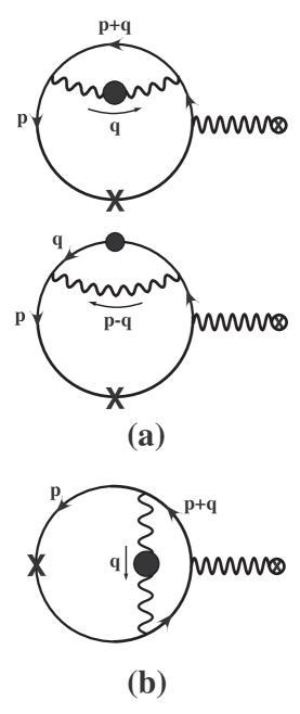
Figure 10: Diagrams contributing to the linearized Boltzmann equation. There are two diagrams of type (a) corresponding to insertions to each side of the self-energy. The solid line denotes the free fermion propagator without the background gauge field. The wiggly line with a circled cross attached to the end denotes to an insertion of the background gauge field. Otherwise, the notation is the same as that in Fig. 9.

The linearized approximation of the Boltzmann equation (147) can be obtained by setting

$$f(\mathbf{p},t)=n_{F}(p)+\delta f(\mathbf{p},t)\;,\quad\overline{f}(-\mathbf{p},t)=n_{F}(p)+\delta\overline{f}(-\mathbf{p},t)\;,$$ (148)

where $\delta f$ and $\delta\overline{f}$ are the departure from equilibrium, and keeping only terms linear in $\delta f$ and $\delta\overline{f}$ in the collision term. Since the collision term vanishes for the equilibrium distribution ($n_{F}$), we find the final form of the linearized Boltzmann equation

$$\frac{\partial}{\partial t}\delta f(\mathbf{p},t)+e\,\bm{\mathcal{E}}\cdot\!\bm{\nabla}_{\mathbf{p}}n_{F}(p) = -2\pi e^{2}\int\frac{d^{3}q}{(2\pi)^{3}}\int^{+\infty}_{-\infty}dq_{0}\bigg{\{}\big{[}K^{+}_{1}(\mathbf{p},\mathbf{q})\;{}^{\ast}\!\rho_{L}(q_{0},q)+K^{+}_{2}(\mathbf{p},\mathbf{q})\;{}^{\ast}\!\rho_{T}(q_{0},q)\big{]}$$ (149)

$$\times\big{[}\delta f(\mathbf{p},t)\;[1+n_{B}(q_{0})-n_{F}(|\mathbf{p}+\mathbf{q}|)]-\delta f(\mathbf{p}+\mathbf{q},t)\;[n_{B}(q_{0})+n_{F}(p)]\big{]}$$

$$\times\,\delta(p-q_{0}-|\mathbf{p}+\mathbf{q}|)+\frac{1}{2|\mathbf{p}-\mathbf{q}|}\big{[}K^{+}_{3}(\mathbf{p},\mathbf{q})\;{}^{\ast}\!\rho_{+}(q_{0},q)+K^{-}_{3}(\mathbf{p},\mathbf{q})\;{}^{\ast}\!\rho_{-}(q_{0},q)\big{]}$$

$$\times\,\delta f(\mathbf{p},t)\;[1+n_{B}(|\mathbf{p}-\mathbf{q}|)-n_{F}(q_{0})]\;\delta(p-q_{0}-|\mathbf{p}-\mathbf{q}|)\bigg{\}}\;.$$

The departure from equilibrium for antiparticles $\delta\overline{f}(-\mathbf{p},t)$ satisfies a similar equation but with the replacement $\delta f(\mathbf{p},t)\to\delta\overline{f}(-\mathbf{p},t)$. We note that the linearized approximation entails that $\delta f$, $\delta\overline{f}\propto\mathcal{E}$, hence the replacement $e\,\bm{\mathcal{E}}\cdot\!\bm{\nabla}_{\mathbf{p}}f(\mathbf{p},t)\to e\,\bm{\mathcal{E}}\cdot\!\bm{\nabla}_{\mathbf{p}}n_{F}(p)$ on the left-hand side of the Boltzmann equation is justified because the neglected term is of second order in $\mathcal{E}$.

V.4 Connection with perturbation theory: the emergence of secular terms

The linearization of the collision term in the Boltzmann equation has a simple and natural interpretation in terms of Feynman diagrams. We recall that the collision term to lowest order is given in Fig. 9, where the fermion propagators are those in the external background field. The linearization corresponds to expanding the propagators to linear order in the background. There are two types of insertions: (i) The external background field is inserted in the fermion lines outside the self-energy (two diagrams), this corresponds to the relaxation time approximation which is manifest by the first term in eq. (149) [proportional to $\delta f(\mathbf{p},t)$] and is depicted in Fig. 10(a). (ii) The insertion is in the fermion propagator inside the self-energy, which corresponds to the second term [proportional to $\delta f(\mathbf{p}+\mathbf{q},t)$] and is depicted in Fig. 10(b). Obviously this last term corresponds to the vertex correction. In fact these diagrams must be compared to those of the self-energy and vertex corrections in the perturbative expansion given in Figs. 3 and 4, respectively, with the external wiggle line in Fig. 10 corresponding to the external photon line in Figs. 3 and 4.

In order to see this relation more clearly, we now show that the perturbative expansion of the solution of the linearized Boltzmann equation (149) reproduces the perturbative results found in Sec. IV.4 above. Let us write the solution of the linearized Boltzmann equation in the following form

$$\delta f(\mathbf{p},t)=e\;\delta f^{(1)}(\mathbf{p},t)+e^{3}\;\delta f^{(2)}(\mathbf{p},t)+\cdots+e^{2n-1}\;\delta f^{(n)}(\mathbf{p},t)+\cdots,$$ (150)

then eq. (149) reduces to

$$\frac{\partial}{\partial t}\delta f^{(1)}(\mathbf{p},t) = -\bm{\mathcal{E}}\cdot\widehat{\mathbf{p}}\;n_{F}^{\prime}(p)\;,$$

$$\frac{\partial}{\partial t}\delta f^{(2)}(\mathbf{p},t) = \delta C[\delta f^{(1)}(\mathbf{p},t)]\;,$$

$$\vdots \vdots$$ (151)

$$\frac{\partial}{\partial t}\delta f^{(n)}(\mathbf{p},t) = \delta C[\delta f^{(n-1)}(\mathbf{p},t)]\;,$$

$$\vdots \vdots$$

where $n_{F}^{\prime}(p)=dn_{F}(p)/dp$ and $\delta C$ denotes the collision term of the linearized Boltzmann equation (149) divided by $e^{2}$. The set of equations (151) can be solved by iteration starting from the lowest order one. Up to order $e^{3}$ we obtain

$$\delta f^{(1)}(\mathbf{p},t) = -t\,\bm{\mathcal{E}}\cdot\widehat{\mathbf{p}}\;n_{F}^{\prime}(p)\;,$$

$$\delta f^{(2)}({\mathbf{p}},t) = 2\pi\left(\frac{t^{2}}{2}\right)\int\frac{d^{3}q}{(2\pi)^{3}}\int^{+\infty}_{-\infty}dq_{0}\bigg{\{}\left[K^{+}_{1}(\mathbf{p},\mathbf{q})\;{}^{\ast}\!\rho_{L}(q_{0},q)+K^{+}_{2}(\mathbf{p},\mathbf{q})\;{}^{\ast}\!\rho_{T}(q_{0},q)\right]$$ (152)

$$\times\big{\{}\bm{\mathcal{E}}\cdot\widehat{\mathbf{p}}\;n_{F}^{\prime}(p)\;[1+n_{B}(q_{0})-n_{F}(|\mathbf{p}+\mathbf{q}|)]-\bm{\mathcal{E}}\cdot\widehat{\mathbf{p}+\mathbf{q}}\;n_{F}^{\prime}(|\mathbf{p}+\mathbf{q}|)\;[n_{B}(q_{0})+n_{F}(p)]\big{\}}$$

$$\times\,\;\delta(p-q_{0}-|\mathbf{p}+\mathbf{q}|)+\frac{1}{2|\mathbf{p}-\mathbf{q}|}\big{[}K^{+}_{3}(\mathbf{p},\mathbf{q})\;{}^{\ast}\!\rho_{+}(q_{0},q)+K^{-}_{3}(\mathbf{p},\mathbf{q})\;{}^{\ast}\!\rho_{-}(q_{0},q)\big{]}$$

$$\times\,\bm{\mathcal{E}}\cdot\widehat{\mathbf{p}}\;n_{F}^{\prime}(p)\;[1+n_{B}(|\mathbf{p}-\mathbf{q}|)-n_{F}(q_{0})]\;\delta(p-q_{0}-|\mathbf{p}-\mathbf{q}|)\bigg{\}}\;.$$

¿From these expressions we can now proceed to compute the current

$$J^{i}(t)=4e\int\frac{d^{3}p}{(2\pi)^{3}}\,\hat{p}^{i}\,\delta f(\mathbf{p},t)\;,$$ (153)

where the factor four accounts for spins, particle and antiparticle. It is more convenient to compute $dJ^{i}(t)/dt$ in order to compare to the perturbative expression of the function $\mathcal{G}^{ij}(t)$. Inserting eq. (152) into eq. (153), we find up to order $e^{4}$ that

$$\frac{d}{dt}J^{i}(t) = -4e^{2}\int\frac{d^{3}p}{(2\pi)^{3}}\;\hat{p}^{i}\;n_{F}^{\prime}(p)\;\bm{\mathcal{E}}\cdot\widehat{\mathbf{p}}+8\pi e^{4}\;t\int\frac{d^{3}p}{(2\pi)^{3}}\;n_{F}^{\prime}(p)\;\bm{\mathcal{E}}\!\cdot\!\widehat{\mathbf{p}}\int\frac{d^{3}q}{(2\pi)^{3}}$$ (154)

$$\times\int^{+\infty}_{-\infty}dq_{0}\;\bigg{\{}(\hat{p}^{i}-\widehat{p+q}^{i})\left[K^{+}_{1}(\mathbf{p},\mathbf{q})\;{}^{\ast}\!\rho_{L}(q_{0},q)+K^{+}_{2}(\mathbf{p},\mathbf{q})\;{}^{\ast}\!\rho_{T}(q_{0},q)\right]$$

$$\times\,[n_{B}(q_{0})+n_{F}(|\mathbf{p}+\mathbf{q}|)]+\frac{\hat{p}^{i}}{2|\mathbf{p}-\mathbf{q}|}\big{[}K^{+}_{3}(\mathbf{p},\mathbf{q})\;{}^{\ast}\!\rho_{+}(q_{0},q)+K^{-}_{3}(\mathbf{p},\mathbf{q})\;{}^{\ast}\!\rho_{-}(q_{0},q)\big{]}$$

$$\times\,[1+n_{B}(|\mathbf{p}-\mathbf{q}|)-n_{F}(q_{0})]\bigg{\}}\;\delta(q_{0}-\widehat{\mathbf{p}}\cdot\mathbf{q})\;.$$

In the above expression we have combined terms of $\mathcal{O}(e^{4})$ that arise from the soft-photon contribution. This is done by relabelling $q_{0}\to-q_{0}$ and using the properties $1+n_{B}(-q_{0})=-n_{B}(q_{0})$ and $\rho_{L,T}(-q_{0},q)=-\rho_{L,T}(q_{0},q)$ in the first term of $\mathcal{O}(e^{4})$, as well as by relabelling $\mathbf{p}\to-\mathbf{p}-\mathbf{q}$ in the second term of this order. Furthermore, we have also used $q\ll p\sim T$ to approximate the argument of the delta functions.

We can now compare the above perturbative expression for $dJ^{i}(t)/dt$ to that obtained from $\mathcal{G}^{ij}(t)$ in Sec. IV.4. With the identification given by eq. (28) it is clear that the term of $\mathcal{O}(e^{2})$ in eq. (154) exactly reproduces the HTL result eq. (33) and that the terms of $\mathcal{O}(e^{4})$ exactly reproduces the two-loop results for the soft-photon and soft-fermion contributions given by eq. (91). Thus we see that the perturbative solution of the linearized Boltzmann equation reproduces the leading secular terms of the perturbative expansion resulting from the self-energy and vertex corrections. The cancellation of the contribution of ultrasoft photon exchange observed at the level of the perturbative expansion is a direct manifestation of the transport time scale that enters in the Boltzmann equation. This exercise not only shows this important result in detail, but it also highlights the following important identifications:

• The term with $\delta f(\mathbf{p},t)$ in the collision term of the linearized Boltzmann equation (149) is associated with the self-energy correction, as manifest in the previous study of the relaxation time approximation.

• The term with $\delta f(\mathbf{p}+\mathbf{q},t)$ in the collision term is associated with the vertex correction. The cancellation between the self-energy and vertex corrections in $q\to 0$ limit, is manifest in the linearized Boltzmann equation (149) as the cancellation between the terms with $\delta f(\mathbf{p},t)$ and $\delta f(\mathbf{p}+\mathbf{q},t)$ [upon using the fact that the photon spectral functions ${}^{\ast}\!\rho_{L,T}(q_{0},q)$ are odd functions of $q_{0}$].

This explicit comparison between the perturbative evaluation of the photon polarization and the perturbative expansion of the solution of the linearized Boltzmann equation (in real time) provides also a justification for ignoring the HTL correction for the vertex [see Fig. 4(b)] at the level of the collision term. This diagram does not contribute to the leading logarithm for linear secular terms in the perturbative expansion, and hence will not contribute leading logarithms to the collision term of the linearized Boltzmann equation.

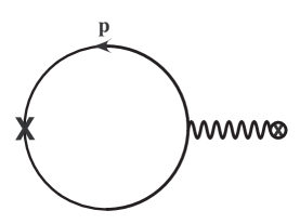
Figure 11: Diagram corresponding to the lowest order perturbative solution $\delta f^{(1)}$ of the linearized Boltzmann equation.

We now argue that the equivalence between the perturbative solution of the linearized Boltzmann equation and the perturbative evaluation of the photon polarization in quantum field theory in real time can be generalized to all orders in perturbation theory, providing a direct identification of the infinite diagrams in the photon polarization that are resummed by the linearized Boltzmann equation. This is achieved by the following observation:

• The lowest order solution $\delta f^{(1)}$ features linear secular term and corresponds diagrammatically to the HTL-type diagram with hard fermion loop, as depicted in Fig. 11.

• The second order solution $\delta f^{(2)}$, which is determined by $\delta C[\delta f^{(1)}]$, features quadratic secular term and corresponds to diagrams obtained from the HTL-type diagram in Fig. 11 by inserting self-energy and vertex corrections, respectively, into the hard fermion lines and the vertex attached to the external wiggly line.

• As discussed in detail in the previous sections, the secular terms with powers $t^{n}$ arise from singular denominators of the form $(\mathbf{k}\cdot{\bf p}-\omega)^{-n}$ for $n=1,2...$ in the limit $\mathbf{k};\omega\rightarrow 0$. In turn these denominators arise from the pinch of two propagators on opposite side of the loop. Thus the iteration above which features powers $t,t^{2},...$ arises from the insertion of uncrossed ladder type diagrams with self-energy corrected side rails. This is the manifestation in real time of the argument provided in referencesjeon ; basagoiti2 that the Boltzmann equation to leading order sums (uncrossed) ladder type diagrams with self-energy corrected side rails.

¿From this observation and the iterative nature of the perturbative solution [see eq. (151)], we conclude by induction that the $n$-th order solution $\delta f^{(n)}$ features secular term of the form $t^{n}$ and the corresponding diagrams is obtained from those of the $(n-1)$-th order solution $\delta f^{(n-1)}$ by performing the same insertion described above. Since the insertion of the vertex correction involves only the vertex attached to the external wiggly line, the only set of diagrams that will be generated are uncrossed ladder diagrams with rainbow type self-energy insertion in the side rails. Consequently, this analysis reveals that the linearized Boltzmann equation (149) resums the uncrossed ladder plus the insertion of rainbow type self-energy diagrams in the photon polarization in accord with the results of reference basagoiti2 ; aarts .

There is an important corollary of the equivalence between the perturbative solution of the linearized Boltzmann equation and the perturbative evaluation of the photon polarization in quantum field theory in real time. Namely, by identifying the contributions at different orders to the linear secular terms in the perturbative expansion of the function $\mathcal{G}(t)$, one can understand precisely what are the diagrams that contribute to the collision term in the linearized Boltzmann equation. In particular, this equivalence allows a direct identification of the contribution from self-energy and vertex corrections to the polarization to the different terms in the linearized Boltzmann equation. Thus, obtaining the linear secular terms in $\mathcal{G}(t)$ yields direct information on the collision term of the linearized Boltzmann equation to all orders in perturbation theory.

Furthermore, this discussion clearly highlights that having proved that the contributions from self-energy and vertex insertions that leading to secular terms fulfill the Ward identity in section (III.5) , the subsequent series resummed by the dynamical renormalization group or Boltzmann equation is fully gauge invariant.

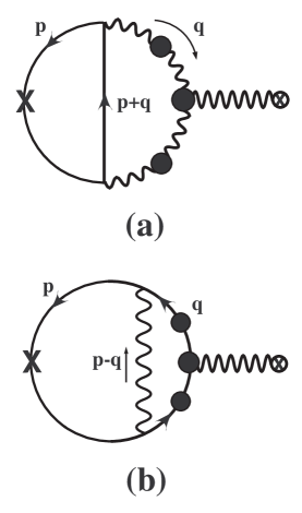
Figure 12: Possible contributions to the linearized Boltzmann equation resulting from a change in the fermion distribution functions that enter the HTL-resummed propagators in (a) the soft-photon contribution and (b) the soft-fermion contribution (see Figs. 9 and 10).

Another important issue that we want to highlight at this point is that the HTL-resummed spectral functions ${}^{\ast}\!\rho_{T,L}$ and ${}^{\ast}\!\rho_{\pm}$ are obtained from the Dyson resummation of the hard thermal loop result, namely these spectral densities are function(als) of the hard fermion distribution functions $f(\mathbf{p},t)$ and $\overline{f}(\mathbf{p},t)$. Thus the question arises: Why did we not account for a change in the fermion distribution functions that enter in the HTL-resummed spectral functions? The answer to this important question is the following: consider such a variation in the hard fermion distribution functions that enter in ${}^{\ast}\!\rho_{L,T}$ and ${}^{\ast}\!\rho_{\pm}$, the resulting contributions are depicted in Fig. 12. For ${}^{\ast}\!\rho_{L,T}$ such contribution would correspond to the vertex correction with a HTL-resummed three-photon vertex [see Fig. 12(a)]. However, such vertex is forbidden by Furry’s theorem, a consequence of CPT invariance in a charge neutral medium (i.e., vanishing fermionic chemical potential) in the absence of a magnetic field. This conclusion is obviously supported by the perturbative expansion, where the absence of such three-photon vertex is manifest. For ${}^{\ast}\!\rho_{\pm}$ such contribution would correspond to the HTL correction for the vertex [see Fig. 12(b)] which is subleading at the leading logarithmic order as we have argued in Secs. IV.3 and IV.4. Thus to leading logarithmic order the departure from equilibrium of the fermion distribution functions are only associated with the hard fermion propagators that generate the kinetic current, and not with the internal fermion propagators that enter in the HTL corrections to the soft photon and fermion propagators.

The Boltzmann equation provides a resummation of these secular divergences. As argued above, by carrying out the perturbative expansion of the Boltzmann equation to higher order and identifying secular terms of the form $t^{n}$ with inverse powers of frequency $\omega^{n+1}$ in the Fourier transform, one can identify what type of the diagrams in the polarization and which parts of the diagrams (e.g., leading logarithms, etc.) that are being resummed. The resummation of diagrams furnished by the Boltzmann equation can thus be put on a similar footing as the resummation of diagrams in the usual renormalization group, where by solving the equation for the running coupling via the renormalization group beta function and expanding this solution in a naive perturbative expansion, one can recognize what type of diagrams and which part of the diagrams are being resummed. Up to the leading logarithmic order considered, the linearized Boltzmann equation resums the leading logarithmic contributions from the uncrossed ladder plus the insertion of rainbow type self-energy diagrams in the photon polarization basagoiti2 ; aarts .

The resummation of the linear secular term in real time is also akin to computing the decay rate in time dependent perturbation theory. By using Fermi’s golden rule to extracts the leading linear secular term at long times and exponentiating the secular term, one obtains the exponential decay of probabilities. This exponentiation is a resummation of the perturbative series.

V.5 Fokker-Planck equation

For soft momentum transfer $q\ll p\sim T$ we can expand the integrand in the collision term of the linearized Boltzmann equation (149) in powers of $q/p$, as we did previously in Sec. IV.4 to obtain the leading logarithms in the perturbative expansion. This expansion, valid for small momentum transfer is akin to that used in astrophysics to obtain the Kompaneets equation from the kinetic equation for the photon distribution function, which is widely used to study inverse Compton scattering by hot electrons lightman . The result is a partial differential equation for the distribution function, a Fokker-Planck equation in momentum space.

The first step in the derivation consists in writing the departure from equilibrium as in eq. (108) in the following form

$$\delta f(\mathbf{p},t)=n_{F}^{\prime}(p)\;\bm{\mathcal{E}}\cdot\widehat{\mathbf{p}}\;\Delta(p,t)\;.$$ (155)

The main reason for this definition is that the inhomogeneous term in the Boltzmann equation is proportional to $n_{F}^{\prime}(p)\;\bm{\mathcal{E}}\cdot\widehat{\mathbf{p}}$. Our analysis of the leading logarithmic contributions in Sec. IV.4 clearly showed that in order to extract the leading logarithms, the transverse and longitudinal photon spectral functions can be replaced by eq. (93) and the momentum integrals must be carried out with an upper cutoff of order $T$ and a lower cutoff of order $eT$. These spectral functions are the perturbative ones, corresponding to just one hard fermion loop in the soft photon and fermion propagators, not the full Dyson series of bubbles. The diagrams that yield the leading logarithmic approximation are depicted in Fig. 13. These diagrams are identified with those of Fig. 6 in the perturbative expansion with the external wiggly line in Fig. 13 corresponding to the external photon line in Fig. 6.

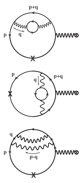
Figure 13: Diagrams that yield the leading logarithmic contribution to the Boltzmann equation.

For $q\ll p$ the argument of the delta functions in the collision term in eq. (149) are approximated by

$$|\mathbf{p}\pm\mathbf{q}|-p=\left\{\pm\,q\,\widehat{\mathbf{p}}\cdot\widehat{\mathbf{q}}+\frac{p}{2}\left(\frac{q}{p}\right)^{2}\left[1-(\widehat{\mathbf{p}}\cdot\widehat{\mathbf{q}})^{2}\right]\right\}\left[1+{\cal O}\left(\frac{q^{3}}{p^{3}}\right)\right]\;,$$ (156)

which simplifies the integral over $q_{0}$ in the collision term in eq. (149). The resulting integrand in the collision term can be expanded in powers of $q/p$. For the soft-photon contribution the leading logarithm arises from terms linear in $q/p$, which leads to a momentum integral of the form $\int^{T}_{eT}dq/q=\ln(1/e)$. Terms of $\mathcal{O}(1)$ in $q/p$ are odd in $\widehat{\mathbf{p}}\cdot\widehat{\mathbf{q}}$ thus vanish after angular integration, while terms of higher order in $q/p$ lead to higher powers of $\alpha$ but not logarithms. For the soft-fermion contribution the leading logarithm arises from terms of $\mathcal{O}(1)$ in $q/p$, which leads to the same momentum integral as for the soft-photon case. Likewise, terms of higher order in $q/p$ lead to higher powers of $\alpha$ but not logarithms.

After some lengthy but straightforward algebra we find the linearized collision term in eq. (149) to be given by

$$C[\Delta]=\frac{e^{4}T^{3}}{24\pi}\ln\left(\frac{1}{e}\right)\bm{\mathcal{E}}\cdot\widehat{\mathbf{p}}\,n_{F}^{\prime}(p)\bigg{[}\Delta^{\prime\prime}(p,t)+\left(\frac{2}{p}-\tanh\frac{p}{2T}\right)\Delta^{\prime}(p,t)-\left(\frac{3}{4pT^{2}}\coth\frac{p}{2T}+\frac{2}{p^{2}}\right)\Delta(p,t)\bigg{]}\;,$$ (157)

where the primes stand for derivatives with respect to $p$. The Boltzmann equation in this approximation becomes the Fokker-Planck equation

$$\frac{1}{e}\frac{\partial}{\partial t}\Delta(p,t)-\frac{e^{3}T^{3}}{24\pi}\ln\left(\frac{1}{e}\right)\bigg{[}\Delta^{\prime\prime}(p,t)+\left(\frac{2}{p}-\tanh\frac{p}{2T}\right)\Delta^{\prime}(p,t)-\left(\frac{3}{4pT^{2}}\coth\frac{p}{2T}+\frac{2}{p^{2}}\right)\Delta(p,t)\bigg{]}=-1\;.$$ (158)

It proves convenient to introduce the transport time scale

$$t_{\mathrm{tr}}=\frac{24\pi}{e^{4}T\ln(1/e)}\;,$$ (159)

and the dimensionless variables,

$$\Phi(x,\tau)\equiv\frac{e^{3}T}{24\pi}\ln\left(\frac{1}{e}\right)\Delta(p,t)\;,\quad\tau\equiv\frac{t}{t_{\mathrm{tr}}}\;,\quad x\equiv\frac{p}{T}\;,$$ (160)

in terms of which the Fokker-Planck equation becomes

$$\dot{\Phi}(x,\tau)-\Phi^{\prime\prime}(x,\tau)-\left(\frac{2}{x}-\tanh\frac{x}{2}\right)\Phi^{\prime}(x,\tau)+\bigg{(}\frac{3}{4x}\coth\frac{x}{2}+\frac{2}{x^{2}}\bigg{)}\Phi(x,\tau)=-1\;,$$ (161)

where the dot and prime stand for derivatives with respect to $\tau$ and $x$, respectively. This equation clearly reveals that the time scale for transport is determined by $t_{\mathrm{tr}}$ defined in eq. (159). The real-time approach leads directly to this Fokker-Planck equation in the leading logarithmic approximation, which reveals at once the transport time scale and includes the time dependence of the departure from equilibrium. Thus this approach has a distinct advantage over the ladder resummation program advocated in Refs. basagoiti1 ; basagoiti2 ; aarts which only captures the asymptotic, steady-state solution.

V.6 Solution of the Fokker-Planck equation: asymptotics

The solution of the Fokker-Planck equation (161) can be written as

$$\Phi(x,\tau)=\phi(x,\tau)+\Phi_{\infty}(x)\;,$$ (162)

where $\phi(x,\tau)$ is a solution of the homogeneous time-dependent Fokker-Planck equation

$$\dot{\phi}(x,\tau)-\phi^{\prime\prime}(x,\tau)-\left(\frac{2}{x}-\tanh\frac{x}{2}\right)\phi^{\prime}(x,\tau)+\bigg{(}\frac{3}{4x}\coth\frac{x}{2}+\frac{2}{x^{2}}\bigg{)}\phi(x,\tau)=0\;,$$ (163)

while, the steady-state solution $\Phi_{\infty}(x)$ obeys the time-independent inhomogeneous equation,

$$\Phi^{\prime\prime}_{\infty}(x)+\left(\frac{2}{x}-\tanh\frac{x}{2}\right)\Phi^{\prime}_{\infty}(x)-\bigg{(}\frac{3}{4x}\coth\frac{x}{2}+\frac{2}{x^{2}}\bigg{)}\Phi_{\infty}(x)=1\;.$$ (164)

Eq.(163) is a parabolic equation that can be solved by expanding ${\phi}(x,\tau)$ in terms of the eigenfunctions $\psi_{n}(x)$ satisfying

$$\left[-\frac{d^{2}}{dx^{2}}-\left(\frac{2}{x}-\tanh\frac{x}{2}\right)\frac{d}{dx}+\frac{3}{4x}\coth\frac{x}{2}+\frac{2}{x^{2}}\right]\psi_{n}(x)=\lambda_{n}\,\psi_{n}(x)$$ (165)

in the interval $0\leq x\leq\infty$ with $\psi_{n}(0)=\psi_{n}(\infty)=0$. Setting

$$\psi_{n}(x)=\frac{\xi_{n}(x)}{x}\cosh\frac{x}{2}\;,$$ (166)

we can rewrite eq. (165) in a Schrödinger-like form

$$\left[-\frac{d^{2}}{dx^{2}}+V(x)\right]\xi_{n}(x)=\lambda_{n}\,\xi_{n}(x)\;,$$ (167)

where

$$V(x)\equiv\frac{1}{4}-\frac{1}{2\,\cosh^{2}\frac{x}{2}}-\frac{1}{x}\tanh\frac{x}{2}+\frac{3}{4x}\coth\frac{x}{2}+\frac{2}{x^{2}}\;.$$ (168)

This potential has a repulsive singularity for $x\to 0$,

$$V(x)\buildrel x\to 0\over{=}\frac{7}{2\;x^{2}}$$ (169)

and for $x\gg 1$ approaches its asymptotic value with an attractive Coulomb tail

$$V(x)\buildrel x\gg 1\over{=}\frac{1}{4}-\frac{1}{4\;x}+\mathcal{O}(e^{-x})\;.$$ (170)

$V(x)$ has its minimum at $x=x_{\mathrm{min}}=15.997\ldots$ with

$$V(x_{\mathrm{min}})=0.2421873\ldots\;,\quad V^{\prime\prime}(x_{\mathrm{min}})=0.0000609\ldots\;.$$ (171)

In addition, $V(x)\geq V(x_{\mathrm{min}})$ and $V^{\prime\prime}(x)>0$ for $0\leq x\leq\infty$.

The Coulomb-like tail of the potential suggests that the spectrum of eq. (165) is formed by an infinite number of discrete eigenvalues with an accumulation point at $\lambda=1/4-0$ and a continuum that starts at $\lambda=1/4$. Therefore the discrete eigenvalues $\lambda_{k}$ (with $k=1,2,3,\ldots$) are in the interval $V(x_{\mathrm{min}})<\lambda_{k}<\frac{1}{4}$. Thus the solution of eq. (163) can be written as,

$$\phi(x,\tau)=\sum_{k}c_{k}\;e^{-\lambda_{k}\,\tau}\;\psi_{k}(x)+\int_{\frac{1}{4}}^{\infty}d\lambda\;c(\lambda)\;e^{-\lambda\;\tau}\;\psi_{\lambda}(x)\;,$$ (172)

where the Fourier coefficients $c_{k}$ and $c(\lambda)$ are obtained from the initial data $\phi(x,0)$ by scalar product with the eigenfunctions. The late times asymptotics is dominated by the ground state,

$$\phi(x,\tau)\buildrel\tau\to\infty\over{=}c_{1}\;e^{-\lambda_{1}\,\tau}\;\psi_{1}(x)\;.$$ (173)

A simple estimate from eq. (171), namely, $\lambda_{1}\approx V(x_{\mathrm{min}})+\sqrt{V^{\prime\prime}(x_{\mathrm{min}})/2}$ suggests that $\lambda_{1}\approx 0.247664$. Therefore, $\Delta(p,t)$ approaches the steady-state solution as

$$\Delta(p,t)\buildrel t\to\infty\over{=}\Delta(p,\infty)+\frac{24\,\pi\,c_{1}}{e^{3}T\ln(1/e)}\;e^{-t/(4.038\ldots\,t_{\mathrm{tr}})}\;\psi_{1}(p)\;.$$ (174)

The steady-state drift current at asymptotically large time $t\gg t_{\mathrm{tr}}$ is given by

$$J^{i}=4\;e\int\frac{d^{3}p}{(2\pi)^{3}}\;\hat{p}^{i}\;\delta f(\mathbf{p})=4e\int\frac{d^{3}p}{(2\pi)^{3}}\;\hat{p}^{i}\;\bm{\mathcal{E}}\cdot\widehat{\mathbf{p}}\;n^{\prime}_{F}(p)\;\Delta(p)=\frac{2}{3}\;e\;\mathcal{E}^{i}\int_{0}^{\infty}dp\;p^{2}\;n^{\prime}_{F}(p)\;\Delta(p)\;,$$ (175)

where the factor $4$ accounts for spin and the fact that the departure from equilibrium for the particle and antiparticle distribution functions are the same. In terms of the steady-state solution $\Phi_{\infty}(x)$ and the dimensionless quantities introduced above in eq. (160), the conductivity is finally given by

$$\sigma=\frac{16\,T}{\pi e^{2}\ln(1/e)}\int_{0}^{\infty}dx\;x^{2}\;n_{F}^{\prime}(x)\;\Phi_{\infty}(x)\;.$$ (176)

¿From the differential equation (164) we can write the following identity

$$\Phi_{\infty}(x)=2\bigg{\{}\Phi_{\infty}(x)-\frac{\Phi_{\infty}(x)}{2}\bigg{[}\Phi^{\prime\prime}_{\infty}(x)+\Phi^{\prime}_{\infty}(x)\left(\frac{2}{x}-\tanh\frac{x}{2}\right)-\bigg{(}\frac{3}{4x}\coth\frac{x}{2}+\frac{2}{x^{2}}\bigg{)}\Phi_{\infty}(x)\bigg{]}\bigg{\}}\;,$$ (177)

which is now inserted in the expression for the conductivity eq. (176). After integration by parts we finally find that

$$\sigma[\Phi_{\infty}]=\frac{32\;T}{\pi e^{2}\ln(1/e)}\int_{0}^{\infty}dx\;n_{F}^{\prime}(x)\bigg{[}\frac{x^{2}}{2}\;\left[\Phi^{\prime}_{\infty}(x)\right]^{2}+\bigg{(}1+\frac{3x}{8}\coth\frac{x}{2}\bigg{)}\;\Phi^{2}_{\infty}(x)+x^{2}\;\Phi_{\infty}(x)\bigg{]}\;.$$ (178)

It is straightforward to confirm that this expression is exactly $2Q[\chi]/3$ given by (4.3) in Ref. arnold after the rescaling of the function $\chi(p)$ in that reference to our dimensionless function $\Phi_{\infty}(x)$. Considering the conductivity as a functional of $\Phi_{\infty}(x)$ given by eq. (178), we find that the variational condition

$$\frac{\delta\,\sigma[\Phi_{\infty}]}{\delta\Phi_{\infty}}=0$$ (179)

leads to the steady-state Fokker-Planck equation (164).

Clearly an analytic solution of the steady-state Fokker-Planck equation (164) is not available. However, before we embark on a numerical study it is important to understand the small and large $x$ behavior of the solution. For this purpose we use the small and large $x$ expansion of the hyperbolic functions. After some algebra we find that the solution regular at the origin has the power expansion

$$\Phi^{<}_{\infty}(x) = a\,H_{<}(x)+I_{<}(x)\;,$$

$$H_{<}(x) = x^{\nu}\left[1+a_{1}\;x^{2}+a_{2}\;x^{4}+{\cal O}(x^{6})\right]\;,$$

$$I_{<}(x) = x^{2}\left[\frac{2}{5}+\frac{3}{110}\;x^{2}+\frac{157}{254100}\;x^{4}+{\cal O}(x^{6})\right]\;,$$ (180)

where

$$\nu=\frac{\sqrt{15}-1}{2}=1.43649\ldots\quad,\quad a_{1}=\frac{32-5\,\sqrt{15}}{176}=0.0717902\ldots\ \quad,\quad a_{2}=\frac{6099-1526\,\sqrt{15}}{84480}=0.00223517\ldots\,.$$ (181)

For $x\gg 1$ the solution that does not grow exponentially is given by

$$\Phi^{>}_{\infty}(x)=b\,H_{>}(x)+I_{>}(x)\;,$$ (182)

where $H_{>}(x)$ has an asymptotic expansion in positive powers of $1/x$ and $e^{-x}$. Neglecting the exponentially small corrections, we find

$$H_{>}(x) \buildrel x\gg 1\over{=} x\;\Psi\left(\frac{7}{4},4;x\right)\left[1+{\cal O}(e^{-x})\right]$$ (183)

$$= x^{-\frac{3}{4}}\bigg{[}1+\sum_{k\geq 1}\frac{(-1)^{k}}{k!\,x^{k}}\left(\frac{7}{4}\right)_{k}\left(-\frac{5}{4}\right)_{k}\bigg{]}\left[1+{\cal O}(e^{-x})\right]$$

$$= x^{-\frac{3}{4}}\left[1+\frac{35}{16\,x}+\frac{385}{512\,x^{2}}+{\cal O}(x^{-3})\right]\left[1+{\cal O}(e^{-x})\right].$$

Here, $\Psi(a,b;z)$ stands for a confluent hypergeometric function gr and $(\mu)_{k}\equiv\mu(\mu+1)\cdots(\mu+k-1)$. The function $I_{>}(x)$ has the asymptotic behavior

$$I_{>}(x)=-\frac{4}{7}\;x+\frac{1}{7}\;e^{-x}+\cdots.$$ (184)

The functions $H_{\lessgtr}(x)$ are the corresponding solutions of the homogeneous equation, while $I_{\lessgtr}(x)$ are the particular solutions of the inhomogeneous equation that are finite at the origin and do not grow exponentially at infinity. The asymptotic linear growth with $x$ of $I_{>}(x)$ is a direct consequence of the inhomogeneity. In addition, the homogeneous equation has a linearly independent (irregular) solution that grows as $x^{-\frac{\sqrt{15}+1}{2}}$ for $x\to 0$.

The coefficients $a$ and $b$ are found by integrating both the homogeneous and inhomogeneous equation with the initial conditions gleaned from eq. (180) on the function and its derivative at the origin for $H_{<}(x)$ and $I_{<}(x)$ and matching the function and derivative to the asymptotic form eqs. (183)-(184) at a value of $x\gg 1$. Such procedure is numerically straightforward, we find that the asymptotic form is achieved for relatively small values of $x\simeq 3$ and the coefficients are found to be given by $a=-0.896\ldots$, $b=-0.01\ldots$. The numerical solution is shown in Fig. 14. With this solution we finally find the following value of the conductivity

$$\sigma=\frac{15.698\,T}{e^{2}\ln(1/e)}\;,$$ (185)

which is consistent with the numerical value quoted in Ref. arnold , $\sigma=\frac{15.6964\,T}{e^{2}\ln(1/e)}$. However we point out that the asymptotic forms for the solution for small or large $x$ are very different from the variational basis chosen in Ref. arnold , in particular near the origin the solution is not an analytic function of $x$.

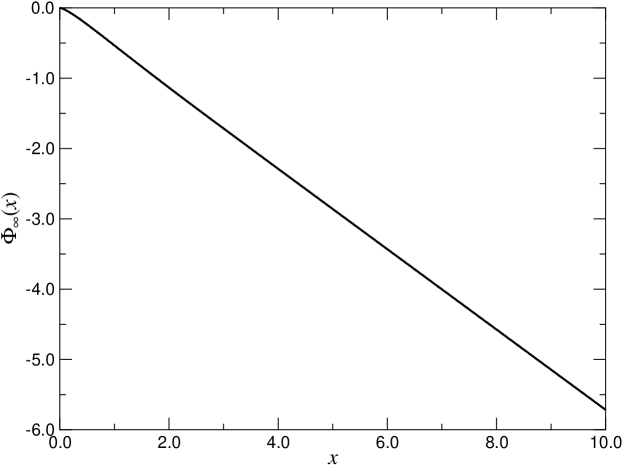
Figure 14: Numerical solution of the steady-state Fokker-Planck equation (164).

V.7 Beyond leading logarithms and the Boltzmann equation

In Sec. IV.4 we have discussed the diagrams that will contribute to next to leading order, which are necessary to fix the constant inside the logarithm for the transport relaxation time and the conductivity. These diagrams will yield new contributions in the collision term. To next to leading order the nonequilibrium fermion distribution function $f$ will replace the equilibrium one $n_{F}$ in the three-loop diagram for the polarization in the soft-fermion contribution $C_{s}^{\mathrm{sf}}$ [see eq. (146)], the collision kernel must also include the first diagram in Fig. 8, the second diagram will arise from linearizing in the departure from equilibrium as discussed above.

The discussion after eq. (100) indicates that the validity of the Boltzmann equation for the evolution of the particle and antiparticle distribution functions is reliable provided processes in which particles and antiparticles mix can be neglected, namely, processes involve momentum exchange $q\ll T$. However, if there are processes that mix particles and antiparticles that lead to secular terms in the perturbative expansion, then the contribution from the spin current in eq. (100) must be accounted for in the evolution equation. In this case one would have to find the equation of motion for the bilinears $\langle b^{\dagger}d^{\dagger}\rangle$, these equations will likely involve the correlators $\langle b^{\dagger}b\rangle$ leading to a coupled system of equations. The new terms are associated with spin precession and in general must be included for a consistent nonequilibrium description heinz . The perturbative analysis and the direct correspondence of the secular terms from the perturbative solution of the Boltzmann equation indicate that such new contributions do not appear at leading logarithmic order. Thus the simpler Boltzmann equation for the particle and antiparticle distribution functions in this leading logarithmic approximation can be interpreted as a low-energy limit of the full set of evolution equations, in the sense that processes that mix particles and antiparticles are neglected.

VI Conclusions

In this article we began a program to study transport phenomena in ultrarelativistic plasmas via the dynamical renormalization group resummation. We focused on the DC electrical conductivity in a ultrarelativistic QED plasma and extracted the conductivity from the long time behavior or a kernel directly related to the retarded photon polarization.

We began by studying the long-time behavior of this kernel in perturbation theory in real time. Pinch singularities in the limit of long wavelength and low frequency that are ubiquitous in the usual perturbative expansion of the imaginary part in the polarization in frequency-momentum space, are manifest as secular terms in real time, namely terms that diverge in the long-time limit. At any finite time the perturbative contributions to the kernel are finite but the long time behavior of the perturbative expansion is divergent reflecting these pinch singularities. We first extracted the leading secular terms at lowest order in the perturbative expansion which includes both self-energy and vertex corrections for the fulfillment of the Ward identity. While the self-energy correction features a logarithmic singularity on the fermion mass shell arising from the exchange of ultrasoft photon which leads to the anomalous damping rate of the hard fermions in the loop, the addition of the vertex correction, as required to fulfill the Ward identity cancels the contributions from the anomalous fermion damping. This cancellation is at the heart of the difference between the quasiparticle and transport relaxation time. We then extracted the leading logarithmic contributions to the leading secular terms and identified the diagrams that yield the leading logarithms and those that yield subleading contributions without logarithms of the coupling.

After the study of the secular divergences in the perturbative expansion, we introduce a resummation program via the dynamical renormalization group applied to the equations of motion of the gauge invariant single-particle distribution functions of hard fermions. The resulting dynamical renormalization group equation in real time is the Boltzmann equation. By expanding the solution of the linearized Boltzmann equation in perturbation theory, we established a direct link between the perturbative expansion of the polarization and the linearized Boltzmann equation by explicitly showing how the Boltzmann equation reproduces the secular terms in a perturbative expansion. This comparison allowed to identify the different terms in the linearized Boltzmann equation with the self-energy and vertex corrections to the polarization. This detailed study leads to a deeper understanding of the resummation of the perturbative series in quantum field theory via the Boltzmann equation. Furthermore, it allows to identify unambiguously the diagrams that contribute to the collision term of the linearized Boltzmann equation. Just as the renormalization group equation in deep inelastic scattering or critical phenomena provides a resummation of parts (such as leading logarithms) of select type of diagrams, the Boltzmann equation also resums parts (leading logarithms) of select diagrams (uncrossed ladder plus rainbow type self-energy corrections).

Thus the dynamical renormalization group provides directly in real time a link between the quantum field theoretical and the Boltzmann kinetic approaches to transport phenomena. Furthermore, we have explicitly shown how the relaxation time approximation of the Boltzmann equation is equivalent to neglecting the vertex corrections in the linearized approximation and features the anomalous logarithmic time dependence manifest in the hard fermion damping rate. The conductivity vanishes in the relaxation time approximation as a consequence of the anomalous logarithms in time. As discussed in Secs. IV.2 and V.2 such an approximation is not valid for the hot QED plasma.

Recognizing that the leading logarithmic contribution to the collision term arises from the region of momentum exchange $eT\lesssim q\lesssim p\sim T$, we expanded the collision kernel of the linearized Boltzmann equation in powers of $q/p$ to extract the leading logarithmic contribution. We then obtained a Fokker-Planck equation in momentum space for the small departure from equilibrium. This equation clearly reveals that the transport time scale is $t_{\mathrm{tr}}=\frac{24\,\pi}{e^{4}T\ln(1/e)}$. The time dependent Fokker-Planck equation is solved by expanding in the eigenfuntions of a positive definite Hamiltonian. For late times, its solution approaches the steady-state solution as $\sim e^{-t/(4.038\ldots\,t_{\mathrm{tr}})}$. We solved analytically the steady-state Fokker-Planck equation for small and large momenta. We matched numerically the solutions and found that the DC conductivity is given by $\sigma=\frac{15.698\,T}{e^{2}\ln(1/e)}$ to leading logarithmic order. This result is within less than $0.1\,\%$ that quoted in Ref. arnold . We established contact with the variational formulation of Refs. arnold ; basagoiti2 ; aarts by showing that the steady-state Fokker-Planck equation can be obtained from a variational functional which is the DC conductivity. We have identified the diagrams that contribute beyond the leading logarithmic order and provided a discussion of the corrections that are necessary to be included in order to go beyond the Boltzmann equation.

The results of this study highlight that the dynamical renormalization group is the concept that provides a direct bridge between quantum field theory and the kinetic description in real time and puts transport phenomena on a similar footing as critical phenomena, namely, the Boltzmann equation is the renormalization group equation that provides a nonperturbative resummation of diagrams. It establishes this formulation as an alternative to studying transport phenomena in relativistic plasmas firmly based on the microscopic quantum field theory. In the next step of our program we will apply these ideas to study transport phenomena in QCD relevant to the physics of the quark-gluon plasma.

Appendix A Imaginary-Time Propagators

In this appendix we review the imaginary-time propagators in their spectral representations. The fermion propagator is given by book:lebellac

$$S(i\omega_{n},\mathbf{p})=\int^{+\infty}_{-\infty}dp_{0}\;\frac{\rho_{F}(p_{0},\mathbf{p})}{p_{0}-i\omega_{n}}\;,$$ (186)

where $\omega_{n}=(2n+1)\pi T$. The spectral function $\rho_{F}(p_{0},\mathbf{p})$ for hard (or free) fermions is given by

$$\rho_{F}(p_{0},\mathbf{p})=\gamma_{+}(\widehat{\mathbf{p}})\;\rho_{+}(p_{0},p)+\gamma_{-}(\widehat{\mathbf{p}})\;\rho_{-}(p_{0},p)\;,$$

$$\gamma_{\pm}(\widehat{\mathbf{p}})=(\gamma^{0}\mp\bm{\gamma}\cdot\widehat{\mathbf{p}})/2\;,\quad\rho_{\pm}(p_{0},p)=\delta(p_{0}\mp p)\;,$$ (187)

where $p=|\mathbf{p}|$, $\widehat{\mathbf{p}}=\mathbf{p}/p$ and $\rho_{\pm}(p_{0},p)$ are the free particle ($+$) and antiparticle ($-$) spectral functions, respectively. The soft (or HTL-resummed) fermion propagator ${}^{\ast}\!S(i\omega,\mathbf{p})$ has the same form as that given in eq. (186) but in terms of the HTL-resummed fermion spectral function,

$${}^{\ast}\!\rho_{F}(p_{0},\mathbf{p})=\gamma_{+}(\widehat{\mathbf{p}})\;{}^{\ast}\!\rho_{+}(p_{0},p)+\gamma_{-}(\widehat{\mathbf{p}})\;{}^{\ast}\!\rho_{-}(p_{0},p)\;,$$

$${}^{\ast}\!\rho_{\pm}(p_{0},p)=Z_{\pm}(p)\;\delta(p_{0}-\omega_{\pm}(p))+Z_{\mp}(p)\;\delta(p_{0}+\omega_{\mp}(p))+\beta_{\pm}(p_{0},p)\;\Theta(p^{2}-p_{0}^{2})\;,$$ (188)

where $Z_{\pm}(p)$ are the residues of the timelike fermionic quasiparticle poles at $\omega_{\pm}(p)$, respectively, and

$$\beta_{\pm}(p_{0},p) = \frac{\frac{m_{f}^{2}}{2p}\big{(}1\mp\frac{p_{0}}{p}\big{)}}{\left\{p\big{(}1\mp\frac{p_{0}}{p}\big{)}\pm\frac{m_{f}^{2}}{2p}\left[\big{(}1\mp\frac{p_{0}}{p}\big{)}\ln\big{|}\frac{p_{0}+p}{p_{0}-p}\big{|}\pm 2\right]\right\}^{2}+\frac{\pi^{2}m_{f}^{4}}{4p^{2}}\big{(}1\mp\frac{p_{0}}{p}\big{)}^{2}}\;,$$ (189)

with $m_{f}^{2}=e^{2}T^{2}/8$ the thermal fermion mass.

The longitudinal and transverse photon propagators are given by

$$D_{L}(i\nu_{n},q) = -\frac{1}{q^{2}}+\int^{+\infty}_{-\infty}dq_{0}\;\frac{\rho_{L}(q_{0},q)}{q_{0}-i\nu_{n}}\;,$$

$$D_{T}(i\nu_{n},q) = \int^{+\infty}_{-\infty}dq_{0}\;\frac{\rho_{T}(q_{0},q)}{q_{0}-i\nu_{n}}\;,$$ (190)

respectively, where $\nu_{n}=2\pi nT$. The frequency independent term is $D_{L}$ arises from the instantaneous Coulomb interaction and is neglected in our calculation because it does not contribute to the imaginary part. For hard photons we have $\rho_{L}=0$ and

$$\rho_{T}(q_{o},q)=\frac{1}{2q}[\delta(q_{0}-q)-\delta(q_{0}+q)]\;.$$ (191)

The soft photon propagators ${}^{\ast}\!D_{L}(i\nu_{n},q)$ and ${}^{\ast}\!D_{T}(i\nu_{n},q)$ have the same form as those given by eq. (190) but in terms of the HTL-resummed spectral functions book:lebellac

$$\rho_{L(T)}(q_{0},q)=\mathrm{sgn}(q_{0})\;Z_{L(T)}(q)\;\delta[q_{0}^{2}-\omega_{s}^{2}(q)]+\beta_{L(T)}(q_{0},q)\;\Theta(q^{2}-q_{0}^{2})\;,$$ (192)

where $Z_{L(T)}(q)$ are the residues of the timelike quasiparticle poles at $\omega_{L(T)}(q)$ and

$$\beta_{L}(q_{0},q) = -\frac{1}{\pi}\frac{\mathrm{Im}\Pi^{\mathrm{HTL}}_{L}(q_{0},q)}{[q^{2}+\mathrm{Re}\Pi^{\mathrm{HTL}}_{L}(q_{0},q)]^{2}+[\mathrm{Im}\Pi^{\mathrm{HTL}}_{L}(q_{0},q)]^{2}}\;,$$

$$\beta_{T}(q_{0},q) = -\frac{1}{\pi}\frac{\mathrm{Im}\Pi^{\mathrm{HTL}}_{T}(q_{0},q)}{[q_{0}^{2}-q^{2}-\mathrm{Re}\Pi^{\mathrm{HTL}}_{T}(q_{0},q)]^{2}+[\mathrm{Im}\Pi^{\mathrm{HTL}}_{T}(q_{0},q)]^{2}}\;.$$ (193)

In the above expressions, $\Pi^{\mathrm{HTL}}_{L(T)}(q_{0},q)$ is the longitudinal (transverse) photon self-energy in the HTL approximation book:lebellac :

$$\Pi^{\mathrm{HTL}}_{L}(q_{0},q) = \frac{e^{2}T^{2}}{6}\left[2-\frac{q_{0}}{q}\ln\left|\frac{q_{0}+q}{q_{0}-q}\right|\right]-i\pi\;\frac{e^{2}T^{2}}{6}\frac{q_{0}}{q}\;\Theta(q^{2}-q_{0}^{2})\;,$$

$$\Pi^{\mathrm{HTL}}_{T}(q_{0},q) = \frac{e^{2}T^{2}}{12}\left[\frac{2q_{0}^{2}}{q^{2}}+\frac{q_{0}}{q}\left(1-\frac{q_{0}^{2}}{q^{2}}\right)\ln\left|\frac{q_{0}+q}{q_{0}-q}\right|\right]-i\pi\;\frac{e^{2}T^{2}}{12}\frac{q_{0}}{q}\left(1-\frac{q_{0}^{2}}{q^{2}}\right)\;\Theta(q^{2}-q_{0}^{2})\;,$$ (194)

The frequency independent part in $D_{L}(i\nu_{n},q)$ and ${}^{\ast}\!D_{L}(i\nu_{n},q)$ arises from the instantaneous Coulomb interaction. Furthermore, we will adopt the convention that bosonic Matsubara frequencies are denoted by $\nu_{m}=2m\pi T$ and the fermionic ones by $\omega_{m}=(2m+1)\pi T$.

The spectral representation of the fermion and photon propagators facilitate the sum over internal Matsubara frequencies. The convenient formulas to carry out these sums systematically are given by book:lebellac

$$T\sum_{\nu_{n}}F(i\nu_{n}) = -\sum_{z_{i}}\mathrm{Res}F(z_{i})\;n_{B}(z_{i})\;,$$

$$T\sum_{\omega_{n}}F(i\omega_{n}) = \sum_{z_{i}}\mathrm{Res}F(z_{i})\;n_{F}(z_{i})\;,$$ (195)

where $\mathrm{Res}$ refers to the residues at the (simple) poles $z_{i}$ of the function $F(z)$, $n_{B}$ is the Bose distribution and $n_{F}$ is the Fermi distribution (for vanishing chemical potential)

$$n_{B}(\omega)=\frac{1}{e^{\omega/T}-1}\;,\quad n_{F}(\omega)=\frac{1}{e^{\omega/T}+1}\;.$$ (196)

Appendix B Real-Time Propagators

In this appendix we summarize the real-time propagators which are used in the main text to derive the quantum Boltzmann equation. The free fermion propagators (with zero chemical potential) are defined by

$$\langle\Psi^{a}(\mathbf{x}{},t)\bar{\Psi}^{b}({\mathbf{x}{}}^{\prime},t^{\prime})\rangle=i\int\frac{d^{3}p}{(2\pi)^{3}}S_{\mathbf{p}}^{ab}(t,t^{\prime})\,e^{i\mathbf{p}\cdot({\mathbf{x}{}}-{\mathbf{x}{}}^{\prime})}\;,$$

$$S_{\mathbf{p}}^{++}(t,t^{\prime})=S_{\mathbf{p}}^{>}(t,t^{\prime})\;\theta(t-t^{\prime})+S_{\mathbf{p}}^{<}(t,t^{\prime})\;\theta(t^{\prime}-t),$$

$$S_{\mathbf{p}}^{--}(t,t^{\prime})=S_{\mathbf{p}}^{>}(t,t^{\prime})\;\theta(t^{\prime}-t)+S_{\mathbf{p}}^{<}(t,t^{\prime})\;\theta(t-t^{\prime})\;,$$

$$S_{\mathbf{p}}^{\pm\mp}(t,t^{\prime})=S_{\mathbf{p}}^{\lessgtr}(t,t^{\prime})\;,$$ (197)

where $\langle\cdots\rangle$ denotes expectation value with respect to the initial density matrix and $a,\;b=\pm$ refer to fields in the forward ($+$) and backward ($-$) time branches. For hard fermions the Wightman functions read

$$S_{\mathbf{p}}^{>}(t,t^{\prime}) = -i\big{\{}\gamma_{+}(\widehat{\mathbf{p}})\;[1-f(\mathbf{p},t_{0})]\;e^{-ip(t-t^{\prime})}+\;\gamma_{-}(\widehat{\mathbf{p}})\;\overline{f}(-\mathbf{p},t_{0})\;e^{ip(t-t^{\prime})}\big{\}}\;,$$

$$S_{\mathbf{p}}^{<}(t,t^{\prime}) = i\big{\{}\gamma_{+}(\widehat{\mathbf{p}})\;f(\mathbf{p},t_{0})\;e^{-ip(t-t^{\prime})}+\;\gamma_{-}(\widehat{\mathbf{p}})\;[1-\overline{f}(-\mathbf{p},t_{0})]\;e^{ip(t-t^{\prime})}\big{\}}\;,$$ (198)

where $f(\mathbf{p},t_{0})$ and $\overline{f}(\mathbf{p},t_{0})$ are the nonequilibrium distribution functions for the hard fermions and antifermions at the initial time $t_{0}$, respectively. For soft fermions the HTL-resummed Wightman functions ${}^{\ast}\!S_{p}^{\gtrless}(t,t^{\prime})$ are expressed in terms of the spectral functions as

$${}^{\ast}\!S_{p}^{>}(t,t^{\prime}) = -i\int^{+\infty}_{-\infty}dq_{0}\,{}^{\ast}\!\rho_{F}(p_{0},p)\,[1-n_{F}(p_{0})]\,e^{-ip_{0}(t-t^{\prime})},$$

$${}^{\ast}\!S_{p}^{<}(t,t^{\prime}) = i\int^{+\infty}_{-\infty}dq_{0}\,{}^{\ast}\!\rho_{F}(p_{0},p)\;n_{F}(p_{0})\;e^{-ip_{0}(t-t^{\prime})},$$ (199)

where ${}^{\ast}\!\rho_{F}(p_{0},p)$ is given by eq. (188).

The longitudinal photon propagators are given by

$$\langle A^{a}_{0}({\mathbf{x}{}},t)A^{b}_{0}({\mathbf{x}{}}^{\prime},t^{\prime})\rangle=i\int\frac{d^{3}q}{(2\pi)^{3}}\,D_{L,q}^{ab}(t,t^{\prime})\;e^{i\mathbf{q}\cdot({\mathbf{x}{}}-{\mathbf{x}{}}^{\prime})}\;,$$

$$D_{L,q}^{++}(t,t^{\prime})=\frac{1}{q^{2}}\;\delta(t-t^{\prime})+D_{L,q}^{>}(t,t^{\prime})\;\theta(t-t^{\prime})+D_{L,q}^{<}(t,t^{\prime})\;\theta(t^{\prime}-t)\;,$$

$$D_{L,q}^{--}(t,t^{\prime})=-\frac{1}{q^{2}}\;\delta(t-t^{\prime})+D_{L,q}^{>}(t,t^{\prime})\;\theta(t^{\prime}-t)+D_{L,q}^{<}(t,t^{\prime})\;\theta(t-t^{\prime})\;,$$

$$D_{L,q}^{\pm\mp}(t,t^{\prime})=D_{L,q}^{\lessgtr}(t,t^{\prime}).$$ (200)

The Wightman functions are expressed in terms of the spectral functions as

$$D_{L,q}^{>}(t,t^{\prime}) = -i\int^{+\infty}_{-\infty}dq_{0}\;\rho_{L}(q_{0},q)\;[1+n_{B}(q_{0})]\;e^{-iq_{0}(t-t^{\prime})}\;,$$

$$D_{L,q}^{<}(t,t^{\prime}) = -i\int^{+\infty}_{-\infty}dq_{0}\;\rho_{L}(q_{0},q)\;n_{B}(q_{0})\;e^{-iq_{0}(t-t^{\prime})}\;.$$ (201)

where $\rho_{L}=0$ for the hard photon propagator and $\rho_{L}={}^{\ast}\!\rho_{L}$ for the soft photon propagator.

The transverse photon propagators are given by

$$\langle A^{i,a}_{T}({\mathbf{x}{}},t)A^{j,b}_{T}({\mathbf{x}{}}^{\prime},t^{\prime})\rangle=-i\int\frac{d^{3}q}{(2\pi)^{3}}\;D_{T,q}^{ab}(t,t^{\prime})\;\mathcal{P}_{T}^{ij}(\mathbf{q})\;e^{i\mathbf{q}\cdot({\mathbf{x}{}}-{\mathbf{x}{}}^{\prime})}\;,$$

$$D_{T,q}^{++}(t,t^{\prime})=D_{T,q}^{>}(t,t^{\prime})\;\theta(t-t^{\prime})+D_{T,q}^{<}(t,t^{\prime})\;\theta(t^{\prime}-t)\;,$$

$$D_{T,q}^{--}(t,t^{\prime})=D_{T,q}^{>}(t,t^{\prime})\;\theta(t^{\prime}-t)+D_{T,q}^{<}(t,t^{\prime})\;\theta(t-t^{\prime})\;,$$

$$D_{T,q}^{\pm\mp}(t,t^{\prime})=D_{T,q}^{\lessgtr}(t,t^{\prime})\;,$$ (202)

where $\mathcal{P}_{T}^{ij}(\widehat{\mathbf{q}})=\delta^{ij}-\hat{q}^{i}\hat{q}^{j}$ is the transverse projector. The Wightman functions are expressed in terms of the spectral functions as

$$D_{T,q}^{>}(t,t^{\prime}) = i\int^{+\infty}_{-\infty}dq_{0}\,{\rho}_{T}(q_{0},q)\;[1+n_{B}(q_{0})]\;e^{-iq_{0}(t-t^{\prime})},$$

$$D_{T,q}^{<}(t,t^{\prime}) = i\int^{+\infty}_{-\infty}dq_{0}\;\rho_{T}(q_{0},q)\;n_{B}(q_{0})\;e^{-iq_{0}(t-t^{\prime})}\;,$$ (203)

where $\rho_{T}=\rho_{B}$ for the hard photon propagator and $\rho_{T}={}^{\ast}\!\rho_{T}$ for the soft photon propagator.

References

- (1) J.-P. Blaizot and J.-Y. Ollitrault, Hydrodynamics of Quark-Gluon Plasmas in Quark-Gluon Plasma, edited by R. Hwa, World Scientific, Singapore, 1990; L.P. Csernai, Introduction to Relativistic Heavy Ion Collisions (John Wiley and Sons, Chichester, 1994); J.A. Maruhn, The Hydrodynamical Model of Heavy Ion Collisions in Relativistic Heavy Ion Physics, edited by L.P. Csernai and D.D. Strottman (World Scientific, Singapore, 1991).
- (2) D. H. Rischke, S. Bernard, and J. A. Maruhn, Nucl. Phys. A 595, 346, 383 (1995); S. Bernard, J.A. Maruhn, W. Greiner, and D. H. Rischke, Nucl. Phys. A 605, 566 (1996); D. Teaney and E. V. Shuryak, Phys. Rev. Lett. 83, 4951 (1999).
- (3) R. Baier, Yu.L. Dokshitzer, A.H. Mueller, and D. Schiff, JHEP 0109, 033 (2001); R. Baier, D. Schiff, and B. G. Zakharov, Ann. Rev. Nucl. Part. Sci. 50, 37 (2000); R. Baier, Yu. L. Dokshitzer, A. H. Mueller and D. Schiff, Phys. Rev. C 60, 064902 (1999).
- (4) C. Hogan, Phys. Rev. Lett. 51,1488 (1983); M.S. Turner and L.M. Widrow, Phys. Rev. D 37, 2743 (1988); K. Enqvist and P. Olesen, Phys. Lett. B 329, 178 (1994); L. Widrow, Rev. Mod. Phys. 74, 775 (2002); M. Giovannini and M.E. Shaposhnikov, Phys. Rev. D 62, 103512 (2000); D. Boyanovsky, H.J. de Vega, and M. Simionato, 67, 023502 (2003); arXiv:hep-ph/0211022.
- (5) G. Baym and H. Heiselberg, Phys. Rev. D 56, 5254 (1997); G. Baym, H. Monien, C.J. Pethick, and D.G. Ravenhall, Phys. Rev. Lett. 64, 1867 (1990); Nucl. Phys. A 525, 415c (1991); G. Baym, H. Heiselberg, C.J. Pethick, and J. Popp, Nucl. Phys. A544, 569c (1992).
- (6) H. Heiselberg, Phys. Rev. D 49, 4739 (1994); H. Heiselberg and C. J. Pethick, 47, R769 (1993); 48, 2916 (1993).
- (7) R. D. Pisarski, Phys. Rev. Lett. 63, 1129 (1989); Physica A 158, 146 (1989); E. Braaten and R.D. Pisarski, Nucl. Phys. B 337, 569 (1990); 339, 310 (1990); R.D. Pisarski, Nucl. Phys. A 525, 175 (1991).
- (8) M. Le Bellac, Thermal Field Theory (Cambridge University Press, Cambridge, 1996).
- (9) P. Arnold, G.D. Moore, and L.G. Yaffe, JHEP 0011, 001 (2000); arXiv:hep-ph/0209353; G.D. Moore, JHEP 0105, 039 (2001); arXiv:hep-ph/0211281.
- (10) See, for example, R. Kubo, M. Toda, and N. Hashitsume, Statistical Physics II: Nonequilibrium Statistical Mechanics, second edition (Springer-Verlag, Berlin, 1991).
- (11) A. Hosoya, M. Sakagami, and M. Takao, Ann. Phys. (N.Y.) 154, 229 (1984).
- (12) S. Jeon, Phys. Rev. D 52, 3591 (1995); S. Jeon and L. G. Yaffe, 53, 5799 (1996); S. Jeon, 47, 4586 (1993); E. Calzetta, B.L. Hu, and S. Ramsey, 61 125013 (2000).
- (13) M. E. Carrington, H. Defu, and R. Kobes, Phys. Lett. B 523,221 (2001); Phys. Rev. D 64 025001 (2001); 62 025010 (2000); E. Calzetta and B. L. Hu, 61 025012 (2000).
- (14) A. Jakovac, Phys. Rev. D 65, 085029 (2002).
- (15) T. Holstein, Ann. Phys. (N.Y.) 29, 410 (1964).
- (16) J. M. Martinez Resco and M. A. Valle Basagoiti, Phys. Rev. D 63, 056008(2001).
- (17) A. L. Selikhov and M. Gyulassy, Phys. Lett. B 316, 373 (1993); P. Arnold and L. G. Yaffe, Phys. Rev. D 62, 125014 (2000).
- (18) M.A. Valle Basagoiti, Phys. Rev. D 66, 045005 (2002).
- (19) G. Aarts and J. M. Martinez Resco, JHEP 0211, 022 (2002).
- (20) E. Mottola and L. M. Bettencourt, The Electrical Conductivity in High Temperature QED in Proceedings of the SEWM2000 Meeting, World Scientific, Singapore, 2001.
- (21) J.-P. Blaizot and E. Iancu, Phys. Rev. Lett. 76, 3080 (1996); Phys. Rev. D 55, 973 (1997); 56, 7877 (1997).
- (22) D. Boyanovsky, H. J. de Vega, R. Holman, and M. Simionato, Phys. Rev. D 60 065003 (1999); D. Boyanovsky and H. J. de Vega, 59 105019 (1999); D. Boyanovsky, H. J. de Vega, and S.-Y. Wang, 61, 065006 (2000).
- (23) S.-Y. Wang, D. Boyanovsky, H. J. de Vega, and D.-S. Lee, Phys. Rev. D 62, 105026 (2000).
- (24) D. Boyanovsky, H. J. de Vega, D.-S. Lee, S.-Y. Wang, and H.-L. Yu, Phys. Rev. D 65, 045014 (2002).
- (25) V.V. Lebedev and A.V. Smilga, Physica A 181, 187 (1992).
- (26) M. Carrington and R. Kobes, Phys. Rev. D 57, 6372 (1998); M. Carrington, R. Kobes, and E. Petitgirard, 57, 2631 (1998).
- (27) U. Kraemmer, A.K. Rebhan, and H. Schulz, Ann. Phys. (N.Y.) 238, 286 (1995); M. Carrington, Phys. Rev. D 48, 3836 (1993).
- (28) P. Aurenche, F. Gelis, and H. Zaraket, JHEP 0207, 063 (2002); and references therein.
- (29) A. Majumder and C. Gale, Phys. Rev. C 65, 055203 (2002).
- (30) R. Baier, B. Pire, and D. Schiff, Phys. Rev. D 38, 2814 (1988); T. Altherr, P. Aurenche and T. Becherrawy, Nucl. Phys. B 315, 436 (1989); T. Altherr and P. Aurenche, Z. Phys. C 45, 99 (1989); J.I. Kapusta and S. M. H. Wong, Phys. Rev. C 62, 027901 (2000).
- (31) See, for instance, G.B. Rybicki and A.P. Lightman, Radiative Processes in Astrophysics (Wiley, New York, 1979).
- (32) P. Zhuang and U. Heinz, Ann. Phys. (N.Y.) 245, 311 (1996); I. Bialynicki-Birula, P. Gornicki, and J. Rafelski, Phys. Rev. D 44, 1825 (1991).
- (33) I.S. Gradshteyn and I.M. Ryshik, Table of Integrals, Series and Products (Academic Press, Boston, 1994); N.N. Lebedev, Special Functions and their Applications (Prentice Hall, Englewood Cliffs, 1965).