Relativistic Unitarized Quark/Meson Model
in Momentum Space

Abstract

An outline is given how to formulate a relativistic unitarized constituent quark model of mesons in momentum space, employing harmonic quark confinement. As a first step, the momentum-space harmonic-oscillator potential is solved in a relativistically covariant, three-dimensional quasipotential framework for scalar particles, using the spline technique. Then, an illustrative toy model with the same dynamical equations but now one $q\bar{q}$ and one meson-meson channel, coupled to one another through quark exchange describing the ${}^{3}P_{0}$ mechanism, is solved in closed form on a spline basis. Conclusions are presented on how to generalize the latter to a realistic multichannel quark/meson model.

1 INTRODUCTION

Mesonic $q\bar{q}$ states are the simplest color-singlet configurations in QCD. However, physical mesons appear to be much more complicated objects, in view of the quite disparate spectra of especially the light scalars and pseudoscalars, and the large variety of states ranging from OZI-stable quarkonia to extremely broad, often badly established resonances. Because of these complexities, theoretical approaches usually focus on parts of the meson data only. Thus, one has quarkonium potential models (see e.g. Ref. [1]), relativistic constituent quark models (see e.g. Ref. [2]), chiral quark models (see e.g. Ref. [3]), heavy-quark effective theory [4], the linear $\sigma$ model (L$\sigma$M) [5], Nambu–Jona-Lasinio models [6], (unitarized) chiral perturbation theory [7]), meson-exchange models (see e.g. Ref. [8]), and so on. While it lies outside the scope of this short paper to describe in detail the respective merits and drawbacks of all these approaches, on can generally state that a good reproduction of either spectra or scattering data is achieved, often at the cost of a non-negligible number of free fit parameters, but without accomplishing a unified description of mesonic spectra and meson-meson scattering. In our view, however, spectra and scattering of mesons are inexorably intertwined concepts, considering that most mesons are resonances, decaying strongly into final states of two or more lighter mesons.

Therefore, we believe one should treat the mechanisms responsible for quark confinement and for mesonic decay on an equal footing. This we have realized already in an essentially non-relativistic (NR) framework, employing the coupled-channel Schrödinger formalism, with several confined $q\bar{q}$ channels and many free two-meson channels. For a detailed discussion of the configuration-space model, we refer to a separate contribution [9] to this workshop, so let us just emphasize here some important non-perturbative features. From the spectroscopic point of view, meson-loop effects on the $q\bar{q}$ spectra are included to all (ladder) orders, even those resulting from closed meson-meson channels. Conversely, the strong influence of $s$-channel $q\bar{q}$ states on non-exotic meson-meson scattering is taken into account. Furthermore, bound states, resonances, and scattering observables all follow directly from an analytic $S$-matrix derived in closed form, thus dispensing with any kind of perturbative methods, which could be highly untrustworthy for the often very large couplings involved. As a matter of fact, perhaps the most remarkable conquest of the model is its parameter-free prediction of the light scalar mesons [10], including the $\kappa$(800) ($K_{0}^{*}$) [11], which has very recently been experimentally confirmed [12]. Precisely for the light scalars, perturbation theory manifestly breaks down [9, 13].

Other coupled-channel, also called unitarized, approaches are due to Eichten et al. (Ref. [1], first paper), Bicudo & Ribeiro (Ref. [3], fourth paper), and Törnqvist with collaborators (Ref. [14] and references therein). The conclusions of the latter two models are in qualitative agreement with ours, in the sense that large shifts are found owing to unitarization, even for (bare) states below the lowest decay threshold. However, in the case of the scalar mesons, important differences between our model and especially the one of Ref. [14] come to light, as the $\kappa$(800) is not found in the latter reference (see Ref. [11] for a detailed comparison).

Notwithstanding its successes, our coordinate-space model has, of course, a number of shortcomings. First of all, the light pseudoscalar mesons are quite badly off, except for the kaon. This may be due to the largely NR formalism without Dirac spin structure , the disregard of chiral symmetry, and possibly also the neglect of scalar-pseudoscalar two-meson channels. Moreover, for most processes, the experimental meson-meson phase shifts are only roughly and not very accurately reproduced, which is no wonder in view of the neglect of final-state interactions from direct $t$-channel meson exchange, and the absence of any “fitting freedom”. Then there are problems with pseudothresholds in heavy-light systems, owing to the non-covariance of minimally relativistic equations in configuration space. Finally, too many, viz. 3, parameters — albeit a very modest number as compared to other approaches — are needed for the ${}^{3}P_{0}$ transition potential, due to the lack of a microscopic description in terms of quark exchange.

Nevertheless, we are convinced one can deal with these shortcomings by reformulating the model in momentum space, in a covariant three-dimensional (3D) quasipotential framework. Here, one could object why we do not attempt to tackle the full Bethe-Salpeter (BS) equation. The reason is twofold: first of all, the numerical effort to solve the resulting coupled 4D integro-differential equations with many channels would be enormous; but perhaps more importantly, the confinement mechanism employing potentials is an inherently 3D concept, possibly leading to a pathological, non-confining behavior when generalized to four dimensions (see e.g. Ref. [2], third paper). Anyhow, a covariant formulation would also allow to include, at a later stage, the Dirac spin structure of the quarks, and address the issue of dynamical chiral-symmetry breaking and generation of constituent mass. The resulting multichannel equations in momentum space we shall show to be explicitly solvable, provided we stick to harmonic confinement and work on a spline basis.

This paper is organized as follows. In Sec. 2 the good old harmonic oscillator (HO) is solved in momentum space using the spline technique, for two different 3D relativistic equations. In Sec. 3 a two-channel toy model, with one harmonically confined $q\bar{q}$ channel coupled via quark exchange to one free two-meson channel, is formally solved in closed form, employing again a spline expansion. Conclusions and an outlook on how to further develop the model are presented in Sec. 4.

2 RELATIVISTIC HARMONIC OSCILLATOR

In this section, we review the well-known 3D HO, first in coordinate space, and then in momentum space. In the latter representation, a 3D relativistic generalization is straightforward.

2.1 Non-Relativistic Harmonic Oscillator

The equal-mass radial Schrödinger equation (SE) for a local potential reads

$$\left\{\frac{1}{m}(-\frac{d^{2}}{dr^{2}}+\frac{l(l+1)}{r^{2}})+V(r)\right\}u(r)\;=\;Eu(r)\;.$$ (1)

If we take the HO potential

$$V(r)\;=\;\frac{1}{2}\mu\,\omega^{2}r^{2}\;,\;\;\;\mu\;=\;\frac{1}{2}m\,,$$ (2)

define $x\equiv\sqrt{\mu\omega}\,r$, and assume for the moment $l=0$, we get

$$\left\{-\frac{d^{2}}{dx^{2}}+x^{2}\right\}u(x)\;=\;\frac{E}{\frac{1}{2}\omega}\ ,u(x)\;.$$ (3)

The spectrum of the 3D HO potential is very well known, viz. ($l=0$)

$$E\;=\;\omega(2n+\frac{3}{2})\;,\;\;\;n=0,1,2,\ldots\,,$$ (4)

leading to the eigenvalues $3,7,11,\ldots$ for Eq. (3).

Alternatively, we can work in momentum space. The homogeneous Lippmann-Schwinger (LS) equation for the bound-state vertex function reads

$$\Gamma(\vec{p})\;=\;\int\frac{d^{3}p^{\prime}}{(2\pi)^{3}}\,V(\vec{p},\vec{p}\,^{\prime})\,G_{0}(\vec{p}\,^{\prime};E)\,\Gamma(\vec{p}\,^{\prime})\;,$$ (5)

where the free two-body Green’s function is given by

$$G_{0}^{-1}(\vec{p}\,^{\prime})\;=\;E-\frac{\vec{p}\,^{\prime 2}}{m}+i\epsilon\;.$$ (6)

Now define the wave function $\Psi\equiv G_{0}\,\Gamma$. Then Eq. (5) becomes

$$G_{0}^{-1}(\vec{p})\Psi(\vec{p})\;=\;\int\frac{d^{3}p^{\prime}}{(2\pi)^{3}}\,V(\vec{p},\vec{p}\,^{\prime})\,\Psi(\vec{p}\,^{\prime})\;,$$ (7)

or equivalently

$$\frac{\vec{p}\,^{2}}{m}\,\Psi(\vec{p})+\int\frac{d^{3}p^{\prime}}{(2\pi)^{3}}\,V(\vec{p},\vec{p}\,^{\prime})\,\Psi(\vec{p}\,^{\prime})\;=\;E\,\Psi(\vec{p})\;.$$ (8)

This is just the SE in momentum space. In this representation, the HO potential is given by

$$V(\vec{p},\vec{p}\,^{\prime})\;=\;-\frac{1}{2}\mu\omega^{2}\,\delta^{(3)}(\vec{p}-\vec{p}\,^{\prime})\,\Delta_{\vec{p}}\;,$$ (9)

which is local as in coordinate space. Substituting into (8) yields

$$\left\{\frac{\vec{p}\,^{2}}{m}\,-\,\frac{1}{2}\mu\omega^{2}\,\Delta_{\vec{p}}\right\}\Psi(\vec{p})\;=\;E\,\Psi(\vec{p})\;.$$ (10)

Taking again $l=0$ and introducing $v(\mbox{p})=\mbox{p}\,\Psi(\mbox{p})$, with $\mbox{p}\equiv|\vec{p}|$, we obtain

$$\left\{\frac{\mbox{p}^{2}}{m}\,-\,\frac{1}{2}\mu\omega^{2}\frac{d^{2}}{d\mbox{p}^{2}}\right\}v(\mbox{p})\;=\;E\,v(\mbox{p})\;.$$ (11)

If we define the dimensionless variable $y\equiv\mbox{p}/\sqrt{\mu\omega}$ and write $m=2\mu$, we get

$$\left\{y^{2}\,-\,\frac{d^{2}}{dy^{2}}\right\}v(y)\;=\;\frac{E}{\frac{1}{2}\omega}\,v(y)\;.$$ (12)

This is identical to Eq. (3). Note that now the roles of the kinetic and the potential term are interchanged.

2.2 Blankenbecler–Sugar–Logunov–Tavkhelidze (BSLT) Equation

The momentum-space equal-mass (scalar) BSLT [15] equation for the wave function has exactly the same form as in the LS case of Eq. (7), but now with center-of-mass (CM) Green’s function

$$G_{0}^{-1}(\vec{p})\;=\;\frac{E_{p}}{m^{2}}\,(\,\frac{s}{4}-E_{p}^{2}+i\epsilon)\;,$$ (13)

where $E_{p}=\sqrt{\vec{p}\,^{2}+m^{2}}$, and $s$ is the total CM energy squared $s=P^{2}=(p_{1}+p_{2})^{2}=(2m+E)^{2}$. Note that $G_{0}^{\mbox{\footnotesize BSLT}}$ can be derived in a completely covariant fashion, and written down explicitly for an arbitrary frame [16]. In the NR limit we have $E_{p}\approx m$ and $s\approx 4m^{2}+4mE$, recovering the LS Green’s function (6). With the new $G_{0}^{-1}$, we get instead of Eq. (8)

$$\frac{\vec{p}\,^{2}}{m}\,\Psi(\vec{p})\,+\,\frac{m}{E_{p}}\int\frac{d^{3}p^{\prime}}{(2\pi)^{3}}\,V(\vec{p},\vec{p}\,^{\prime})\,\Psi(\vec{p}\,^{\prime})\;=\;\frac{s-4m^{2}}{4m}\>\Psi(\vec{p})\;.$$ (14)

In terms of the above-defined dimensionless variable $y$, the BSLT equation becomes

$$\left\{y^{2}\,-\,\frac{1}{\displaystyle\sqrt{1+\frac{\omega}{2m}y^{2}}}\,\frac{d^{2}}{dy^{2}}\right\}v(y)\;=\;\frac{s-4m^{2}}{2m\omega}\>v(y)\,.$$ (15)

From this equation we readily see that deviations from the LS case are determined by the parameter $\omega/2m$. Furthermore, in the limit $\omega/2m\rightarrow 0$, the eigenvalues $3,7,11,\ldots$ get recovered. However, there are additional relativistic effects due to $s\neq 4m^{2}+4mE$.

2.3 Equal-Time (ET) Equation

The ET, also called Mandelzweig–Wallace [17], Green’s function can be obtained from the BSLT (or Salpeter) equation by adding an extra term $G_{0}^{C}$ to the two-body Green’s function $G_{0}$ which approximates crossed-ladder contributions. This extra term becomes exact in the eikonal limit, or when one of the particles gets infinitely heavy. Therefore, the covariant ET equation manifestly has the correct one-body limit, i.e., one recovers either the Klein–Gordon or the Dirac equation, for scalar or spin-1/2 particles, respectively. In the scalar case, the CM ET Green’s function is given by

$$G_{0}^{-1}(\vec{p})\;=\;\frac{E_{p}^{3}}{m^{2}}\;\frac{\displaystyle\frac{s}{4}-E_{p}^{2}+i\epsilon}{2E_{p}^{2}-\displaystyle\frac{s}{4}}\;.$$ (16)

The final form of the $S$-wave ET equation for the HO potential in momentum space reads

$$\left\{y^{2}\,-\,\frac{1}{\displaystyle\sqrt{1+\frac{\omega}{2m}y^{2}}}\left[2-\frac{1}{\displaystyle\displaystyle 1+\frac{\omega}{2m}y^{2}}\right]\frac{d^{2}}{dy^{2}}\right\}v(y)\;=\;\frac{s-4m^{2}}{2m\omega}\>\left\{1\,-\,\frac{\displaystyle\frac{\omega}{2m}}{\left(\displaystyle 1+\frac{\omega}{2m}\right)^{\frac{3}{2}}}\,\frac{d^{2}}{dy^{2}}\right\}v(y)\;.$$ (17)

2.4 Non-Zero Orbital Angular Momentum

For $l\neq 0$, the dimensionless LS equation becomes

$$\left\{-\frac{d^{2}}{dx^{2}}\,+\,\frac{l(l+1)}{x^{2}}\,+\,x^{2}\right\}u(x)\;=\;\frac{E}{\frac{1}{2}\omega}\,u(x)\;.$$ (18)

In order to numerically solve the LS and corresponding BSLT, ET equations, we substitute $u(x)\rightarrow x^{l}\tilde{u}(x)$. Then

$$\left\{-\frac{d^{2}}{dx^{2}}\,+\,\frac{2l}{x^{2}}(1-x\frac{d}{dx})\,+\,x^{2}\right\}\tilde{u}(x)\;=\;\frac{E}{\frac{1}{2}\omega}\,\tilde{u}(x)\;.$$ (19)

The function $\tilde{u}(x)$ has the right boundary conditions to allow an easy numerical solution using an expansion on a spline basis (for details, see Ref. [18] and second paper of Ref. [2]). Thus, the NR HO spectrum is recovered with great accuracy, viz.

$$E\;=\;\omega\,(2n\,+\,l\,+\,\frac{3}{2})\;,\,\;\;\;n,l=0,1,2,\ldots\;.$$ (20)

Figure 1: Dimensionless energy levels of the HO for the LS, BSLT, and ET equations, as a function of $\omega/m_{q}$; first three radial levels are depicted ($l=0$).

In the case of the BSLT and ET equations, the same can be done by replacing everywhere

$$-\frac{d^{2}}{dy^{2}}\;\longrightarrow\;\frac{2l}{y^{2}}\,(1-y\frac{d}{dy})\,-\,\frac{d^{2}}{dy^{2}}\;.$$ (21)

The LS, BSLT, and ET results for $l=0$ are depicted in Fig. 1. We see that the relativistic corrections are relatively modest for the BSLT equation, but can become huge in the ET case, especially for excited states. The latter large effect has to do with the sign change of the ET propagator (16) as a function of the relative momentum, and has also been observed in the Dirac case (see Ref. [2], second paper). However, this overshooting of the ET equation will strongly depend on the chosen Dirac structure of the confining force in a realistic model, and hence should not cause any worries at this stage.

3 UNITARIZED MODEL IN MOMENTUM SPACE

Consider now a simple two-channel model of one confined $q\bar{q}$ system coupled to one free meson-meson channel. In a unitarized picture, this can formally be described by a $2\!\times\!2\,$ $T$ matrix, with the dynamical equation (LS, BSLT, or ET)

$$\left(\begin{array}[]{cc}T_{00}&T_{01}\\ T_{10}&T_{11}\end{array}\right)\;=\;\left(\begin{array}[]{cc}V_{00}&V_{01}\\ V_{10}&V_{11}\end{array}\right)\>+\>\left(\begin{array}[]{cc}V_{00}&V_{01}\\ V_{10}&V_{11}\end{array}\right)\left(\begin{array}[]{cc}G_{0}&0\\ 0&G_{1}\end{array}\right)\left(\begin{array}[]{cc}T_{00}&T_{01}\\ T_{10}&T_{11}\end{array}\right)\;.$$ (22)

Equation (22) is diagrammatically represented in Fig. 2.

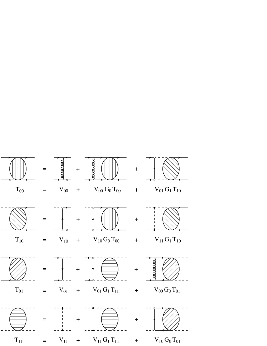
Figure 2: Graphical representation of Eq. (22); see text for explanation.

Dashed lines are mesons, solid lines with arrows are (anti)quarks, and curly exchanges symbolize confinement. Furthermore, open circles represent meson-quark-antiquark vertices, and dots stand for three-meson vertices. Note that the communication between the $q\bar{q}$ and two-meson channels takes place through quark exchange. This will give rise to a generally non-local ${}^{3}P_{0}$ transition potential in configuration space, as soon as the quarks and mesons have different masses. The precise form of such a potential will also depend on possible form factors to be attributed to the various vertices.

In order to solve Eq. (22), we must realize that no asymptotic scattering of quarks is possible, so $T_{00}$, $T_{01}$, and $T_{10}$ must in the end be eliminated from the equations: only $T_{11}$ can be on shell. If we now take again harmonic confinement, Eq. (22) becomes a set of coupled integro-differential equations. Omitting for clarity angular-momentum indices, we get e.g. for $T_{01}$

$$T_{01}(\mbox{p},\mbox{p}^{\prime})\;=\;V_{01}(\mbox{p},\mbox{p}^{\prime})\,-\,\frac{1}{2}\mu\omega^{2}\Delta_{\mbox{\footnotesize p}}\,G_{0}(\mbox{p})\,T_{01}(\mbox{p},\mbox{p}^{\prime})\,+\,\int\frac{\mbox{k}^{2}d\mbox{k}}{4\pi^{2}}\,V_{01}(\mbox{p},\mbox{k})\,G_{1}(\mbox{k})\,T_{11}(\mbox{k},\mbox{p}^{\prime})\;.$$ (23)

Note that $\mbox{p}^{\prime}$ is an essentially dummy variable in the equations, so we can choose a fixed value for it, say $\bar{\mbox{p}}$. If we now expand $T_{01}$ and $T_{11}$ on a spline basis and discretize the initial momentum p, then $T_{01}$ can be expressed in terms of $T_{11}$ as follows.

$$T_{01}(\mbox{p}_{i},\bar{\mbox{p}})\;=\;\sum_{j=1}^{N}t_{01}^{j}s_{01}^{j}(\mbox{p}_{i})\;,\;\;\;v_{01}^{i}\;\equiv\;V_{01}(\mbox{p}_{i},\bar{\mbox{p}})\;;$$ (24)

$$T_{11}(\mbox{k},\bar{\mbox{p}})\;=\;\sum_{j=1}^{N}t_{11}^{j}s_{11}^{j}(\mbox{k})\;;$$ (25)

$$A_{01}^{ij}\;\equiv\;\left\{1\,+\,\frac{1}{2}\mu\omega^{2}\,\Delta_{\mbox{\footnotesize p}_{i}}\,G_{0}(\mbox{p}_{i})\right\}s_{01}^{j}(\mbox{p}_{i})\;;$$ (26)

$$A_{11}^{ij}\;\equiv\;\int\frac{\mbox{k}^{2}d\mbox{k}}{4\pi^{2}}\,V_{01}(\mbox{p}_{i},\mbox{k})\,G_{1}(\mbox{k})\,s_{11}^{j}(\mbox{k})\;.$$ (27)

Combining Eqs. (24)–(27), we can write

$${\bf A}_{01}\cdot{\bf t}_{01}\;=\;{\bf v}_{01}\,+\,{\bf A}_{11}\cdot{\bf t}_{11}\;\;\Rightarrow\;\;{\bf t}_{01}\;=\;{\bf A}_{01}^{-1}\cdot\{{\bf v}_{01}\,+\,{\bf A}_{11}\cdot{\bf t}_{11}\}\;,$$ (28)

where the boldface capitals and small letters are obvious shorthands for matrices and vectors, respectively. Turning next to $T_{11}$, we get the integral equation

$$T_{11}(\mbox{p},\bar{\mbox{p}})\;=\;V_{11}(\mbox{p},\bar{\mbox{p}})\,+\,\int\frac{\mbox{k}^{2}d\mbox{k}}{4\pi^{2}}\,V_{11}(\mbox{p},\mbox{k})\,G_{1}(\mbox{k})\,T_{11}(\mbox{k},\bar{\mbox{p}})\,+\,\int\frac{\mbox{k}^{2}d\mbox{k}}{4\pi^{2}}\,V_{10}(\mbox{p},\mbox{k})\,G_{0}(\mbox{k})\,T_{01}(\mbox{k},\bar{\mbox{p}})\;.$$ (29)

Similarly to Eqs. (24)–(27), we define now

$$B_{11}^{ij}\;\equiv\;s_{11}^{j}(\mbox{p}_{i})\,-\,\int\frac{\mbox{k}^{2}d\mbox{k}}{4\pi^{2}}\,V_{11}(\mbox{p}_{i},\mbox{k})\,G_{1}(\mbox{k})s_{11}^{j}(\mbox{k})\;;$$ (30)

$$B_{01}^{ij}\;\equiv\;\int\frac{\mbox{k}^{2}d\mbox{k}}{4\pi^{2}}\,V_{10}(\mbox{p}_{i},\mbox{k})\,G_{0}(\mbox{k})\,s_{01}^{j}(\mbox{k})\;,\;\;\;v_{11}^{i}\;\equiv\;V_{11}(\mbox{p}_{i},\bar{\mbox{p}})\;.$$ (31)

Then we can express ${\bf t}_{11}$ in terms of itself, using Eq. (28):

$${\bf B}_{11}\cdot{\bf t}_{11}\;=\;{\bf v}_{11}\,+\,{\bf B}_{01}\cdot{\bf t}_{01}\;\;\raisebox{-8.53581pt}{$\stackrel{{\scriptstyle\displaystyle=}}{{\scriptstyle(28)}}$}\;\;{\bf v}_{11}\,+\,{\bf B}_{01}\cdot{\bf A}_{01}^{-1}\cdot\{{\bf v}_{01}\,+\,{\bf A}_{11}\cdot{\bf t}_{11}\}\;.$$ (32)

This finally leads to

$$\{{\bf B}_{11}\,-\,{\bf B}_{01}\cdot{\bf A}_{01}^{-1}\cdot{\bf A}_{11}\}\cdot{\bf t}_{11}\;=\;{\bf v}_{11}\,+\,{\bf B}_{01}\cdot{\bf A}_{01}^{-1}\cdot{\bf v}_{01}\;,$$ (33)

$${\bf t}_{11}\;=\;\{{\bf B}_{11}\,-\,{\bf B}_{01}\cdot{\bf A}_{01}^{-1}\cdot{\bf A}_{11}\}^{-1}\>\cdot\>\{{\bf v}_{11}\,+\,{\bf B}_{01}\cdot{\bf A}_{01}^{-1}\cdot{\bf v}_{01}\}\;.$$ (34)

Thus, we have obtained a closed-form expression for the $T$ matrix (hence the $S$ matrix), containing the complete information of the confinement-plus-scattering process. Needless to say that all these algebraic manipulations only make sense if the involved integrals actually exist and the spline expansions converge. Yet, we are confident this will be the case when appropriate boundary conditions are chosen, since the same spline expansion we are using here has been successfully applied to few-body scattering calculations in momentum space [19]. Nevertheless, in the Dirac case, to be dealt with in the future, form factors will have to be included for the meson-quark-antiquark vertices so as to make the integrals involving three quark propagators convergent. In any case, such form factors are physically meaningful, and should therefore already be considered in the approximation with spinless fermions, whenever doing phenomenology.

Bound states and resonances are given by zeroes in the determinant of the inverted-matrix factor right after the equal sign in Eq. (34). Resonance poles in the second Riemann sheet can be searched for by analytic continuation to complex energies, using e.g. contour-rotation methods. Moreover, from the structure of the equations one readily sees that the inclusion of final-state interactions, due to $t$-channel meson exchange in the meson-meson channel, simply amounts to taking a non-vanishing $V_{11}$ in Eq. (29), which will not lead to any additional numerical effort. Finally, the generalization to many scattering channels and also more $q\bar{q}$ channels is straightforward, at the expense of bigger matrices.

4 CONCLUSIONS AND OUTLOOK

In the foregoing, we have demonstrated that the formulation of a unitarized quark/meson model with harmonic confinement is relatively easy in momentum space. Thus, the ${}^{3}P_{0}$ mechanism is dynamically described through $P$-wave quark exchange. Furthermore, the inclusion of final-state interactions via $t$-channel meson exchange is straightforward, and does not complicate the structure of the equations. The numerical resolution of these equations using splines looks very convenient, which should result in (approximate) analytic solutions, thereby facilitating an analytic continuation to complex energies in order to search for resonance poles.

Our first priority is, of course, to achieve a total control of the numerics, for real as well as complex energy. Then a simple toy model will be worked out so as to reproduce known coordinate-space results. Furthermore, cases problematic in the configuation-space formulation will be studied, such as heavy-light mesons. Also, the influence of $t$-channel meson exchange on meson-meson phase shifts will be investigated. In a somewhat more distant perspective, we intend to do a lot of phenomenology, and use the feedback to further refine the model.

Acknowledgments The authors thank F. Kleefeld and J. A. Tjon for valuable discussions, and P. Nogueira for expert graphical assistance. This work was partly supported by the Fundação para a Ciência e a Tecnologia (FCT) of the Ministério do Ensino Superior, Ciência e Tecnologia of Portugal, under contract number CERN/P/FIS/43697/2001.

References

- [1] E. Eichten, K. Gottfried, T. Kinoshita, K. D. Lane, and T. M. Yan, Phys. Rev. D 21, 203 (1980); J. L. Richardson, Phys. Lett. B 82, 272 (1979).
- [2] S. Godfrey and N. Isgur, Phys. Rev. D 32 (1985) 189; P. C. Tiemeijer and J. A. Tjon, Phys. Rev. C 49, 494 (1994); P. C. Tiemeijer, Ph.D. Thesis, Utrecht (1993).
- [3] A. Le Yaouanc, L. Oliver, S. Ono, O. Pene and J. C. Raynal, Phys. Rev. D 31, 137 (1985); P. J. Bicudo and J. E. Ribeiro, Phys. Rev. D 42, 1611 (1990); 42, 1625 (1990); 42, 1635 (1990).
- [4] N. Isgur and M. B. Wise, Phys. Rev. Lett. 66, 1130 (1991); M. Neubert, Phys. Rept. 245, 259 (1994) [hep-ph/9306320].
- [5] M. Gell-Mann and M. Lévy, Nuovo Cim. 16, 705 (1960); R. Delbourgo and M. D. Scadron, Mod. Phys. Lett. A 10, 251 (1995) [hep-ph/9910242]; Int. J. Mod. Phys. A 13, 657 (1998) [hep-ph/9807504].
- [6] Y. Nambu and G. Jona-Lasinio, Phys. Rev. 122, 345 (1961); V. Bernard, A. H. Blin, B. Hiller, Y. P. Ivanov, A. A. Osipov, and U. G. Meissner, Annals Phys. 249, 499 (1996) [hep-ph/9506309].
- [7] J. Gasser and H. Leutwyler, Annals Phys. 158, 142 (1984); J. A. Oller, E. Oset, and J. R. Peláez, Phys. Rev. D59 (1999) 074001 [Erratum-ibid. D60 (1999) 099906] [hep-ph/9804209].
- [8] D. Lohse, J. W. Durso, K. Holinde, and J. Speth, Nucl. Phys. A 516, 513 (1990).
- [9] E. v. Beveren, G. Rupp, N. Petropoulos, and F. Kleefeld, hep-ph/0211411.
- [10] E. van Beveren, T. A. Rijken, K. Metzger, C. Dullemond, G. Rupp, and J. E. Ribeiro, Z. Phys. C30, 615 (1986).
- [11] E. van Beveren and G. Rupp, Eur. Phys. J. C 10, 469 (1999) [hep-ph/9806246].
- [12] E. M. Aitala et al. [E791 Collaboration], Phys. Rev. Lett. 89, 121801 (2002) [hep-ex/0204018].
- [13] E. van Beveren and G. Rupp, Eur. Phys. J. C 22, 493 (2001) [hep-ex/0106077].
- [14] Nils A. Törnqvist and Matts Roos, Phys. Rev. Lett. 76 (1996) 1575 [hep-ph/9511210].
- [15] A. A. Logunov and A. N. Tavkhelidze, Nuovo Cim. 29 (1963) 380; R. Blankenbecler and R. Sugar, Phys. Rev. 142, 1051 (1966).
- [16] R. M. Woloshyn and A. D. Jackson, Nucl. Phys. B 64, 269 (1973).
- [17] S. J. Wallace and V. B. Mandelzweig, Nucl. Phys. A 503, 673 (1989).
- [18] G. L. Payne, Lect. Notes Phys. 273, 64 (1987).
- [19] M. T. Peña, H. Garcilazo, P. U. Sauer, and U. Oelfke, Phys. Rev. C 45, 1487 (1992).