$B\rightarrow\phi K_{S}$ and supersymmetry

Abstract

The rare decay $B\to\phi K_{S}$ is a well-known probe of physics beyond the Standard Model because it arises only through loop effects yet has the same time-dependent CP asymmetry as $B\to\psi K_{S}$. Motivated by recent data suggesting new physics in $B\to\phi K_{S}$, we look to supersymmetry for possible explanations, including contributions mediated by gluino loops and by Higgs bosons. Chirality-preserving $LL$ and $RR$ gluino contributions are generically small, unless gluinos and squarks masses are close to the current lower bounds. Higgs contributions are also too small to explain a large asymmetry if we impose the current upper limit on $B(B_{s}\rightarrow\mu^{+}\mu^{-})$. On the other hand, chirality-flipping $LR$ and $RL$ gluino contributions can provide sizable effects and while remaining consistent with related results in $B\to\psi K_{S}$, $\Delta M_{s}$, $B\rightarrow X_{s}\gamma$ and other processes. We discuss how the $LR$ and $RL$ insertions can be distinguished using other observables, and we provide a string-based model and other estimates to show that the needed sizes of mass insertions are reasonable.

I Introduction

$B\to\phi K_{S}$ is a powerful testing ground for new physics. Because it does not occur at tree level in the standard model (SM), but only via loop contributions, this decay is very sensitive to possible new physics contributions to the quark level process $b\rightarrow ss\bar{s}$. Within the SM, it is dominated by the QCD (and electroweak) penguin diagrams with a top quark in the loop (see Fig. 1). Therefore the time dependent CP asymmetries are essentially due to $B^{0}$–$\bar{B}^{0}$ mixing and thus are the same as those in $B\to\psi K_{S}$: $\sin 2\beta_{\phi K}\simeq\sin 2\beta_{\psi K}+O(\lambda^{2})$ worah .

Recently the $B\to\phi K_{S}$ decay was observed by both BaBar and Belle at the branching ratio of $\sim(8-9)\times 10^{-6}$ (see Table 1). This is in accord with theoretical predictions based on various factorization approximations, albeit there are considerable uncertainties in theoretical predictions. Being a penguin dominated process, the theoretical prediction for the branching ratio of $B\to\phi K_{S}$ is very sensitive to the so-called effective number of colors $N_{c}^{\rm eff}$, which has been widely used in the old factorization approximations akl1 . Varying $N_{c}^{\rm eff}$ from 2 to $\infty$, the predicted branching ratio lies in the range $13\times 10^{-6}$ and $0.4\times 10^{-6}$ hycheng1 . If one uses the improved QCD factorization method developed by Beneke, Buchalla, Neubert and Sachrajda (BBNS) bbns (where $N_{c}^{\rm eff}=N_{c}=3$), one obtains $B(B\to\phi K^{0})\simeq 5\times 10^{-6}$, somewhat lower than the current world average despite large experimental uncertainties. Another approach based on perturbative QCD yields the branching ratio of this decay at the level of $10\times 10^{-6}$ within the SM keum . On the other hand, the CP asymmetries in $B\to\phi K_{S}$ are less model dependent, since they are ratios of branching ratios for $B^{0}$ and $\bar{B}^{0}$ decays. Large theoretical uncertainties mostly cancel out between the numerator and the denominator (see, e.g., Ref. akl2 ).

In general, the time dependent CP asymmetry in $B^{0}(\bar{B}^{0})\rightarrow\phi K_{S}$ (or for any common CP eigenstates into which both $B^{0}$ and $\bar{B}^{0}$ can decay) measures two independent pieces of information nir :

$${\cal A}_{\phi K}(t) \equiv {{\Gamma(\bar{B}^{0}_{\rm phys}(t)\rightarrow\phi K_{S})-\Gamma(B^{0}_{\rm phys}(t)\rightarrow\phi K_{S})}\over{\Gamma(\bar{B}^{0}_{\rm phys}(t)\rightarrow\phi K_{S})+\Gamma(B^{0}_{\rm phys}(t)\rightarrow\phi K_{S})}}$$ (1)

$$= -C_{\phi K}\cos(\Delta Mt)+S_{\phi K}\sin(\Delta Mt),$$

where $C_{\phi K}$ and $S_{\phi K}$ are given by

$$C_{\phi K}={1-|\lambda_{\phi K}|^{2}\over 1+|\lambda_{\phi K}|^{2}},~{}~{}~{}~{}~{}{\rm and}~{}~{}~{}~{}~{}S_{\phi K}={2~{}{\rm Im}\lambda_{\phi K}\over 1+|\lambda_{\phi K}|^{2}},$$ (2)

with

$$\lambda_{\phi K}\equiv-e^{-2i(\beta+\theta_{d})}{\bar{A}(\bar{B}^{0}\to\phi K_{S})\over A(B\to\phi K_{S})}.$$ (3)

The angles $\beta$ and $\theta_{d}$ represent the SM and any new physics contributions to the $B^{0}$–$\bar{B}^{0}$ mixing angle; we will assume the latter to be small. $A(B\to\phi K_{S})$ is the amplitude for the nonleptonic $B$ decay of interest. If there are several independent channels relevant to the same final states with weak phases $\varphi_{m}$ and strong phases $\delta_{m}$ (with $m=1,2,\ldots$ labeling different channels), the decay amplitude $A$ for a particle is given by

$$A=\sum_{m}a_{m}e^{+i\varphi_{m}}e^{+i\delta_{m}},$$ (4)

whereas the decay amplitude $\bar{A}$ for the antiparticle is given by

$$\overline{A}=\sum_{m}a_{m}e^{-i\varphi_{m}}e^{+i\delta_{m}}.$$ (5)

Here $a_{m}>0$ is the modulus of the amplitude of the $m$-th channel. Within the SM, the amplitude is real to a good accuracy so that $\lambda_{\phi K}=-e^{-2i\beta}=\lambda_{\psi K}$. This remains true if any new physics contributions are real relative to the SM decay amplitude for $B\to\phi K_{S}$. Therefore one needs a new CP violating phase(s) $\varphi_{m}$ if there exists any significant deviation of $S_{\phi K}$ from $S_{\psi K}$. For example, if there is a new physics contribution to the decay with amplitude whose modulus is $a_{\rm NP}$, weak phase is $\varphi$ and strong phase is $\delta$, then

$$\lambda_{\phi K}=-e^{-2i(\beta+\theta_{d})}{1+re^{i(\delta-\varphi)}\over 1+re^{i(\delta+\varphi)}}\,\,\stackrel{{\scriptstyle r\gg 1}}{{\longrightarrow}}\,-e^{-2i(\beta+\theta_{d}+\varphi)},$$ (6)

where $r\equiv a_{\rm NP}/a_{\rm SM}$. In general, the strong phase $\delta$ will affect both $S_{\phi K}$ and $C_{\phi K}$. However if the new physics contributions dominate over the SM ones, the strong phase effectively drops out, an approach that is commonly (and mistakenly) used in the literature even when $r$ is not large. We will comment further on the nature and source of the strong phases in Section III.

Table 1: CP averaged branching ratios, $S_{\phi K}$ and $C_{\phi K}$ in $B\to\phi K_{S}$ from BaBar babar ; lp03 and Belle belle ; lp03 and the SM predictions in the BBNS approach.

Observable	BaBar	Belle	Average	SM prediction
$Br$ (in $10^{-6}$)	$8.1\,{}^{+3.1}_{-2.5}\pm 0.8$	$8.7\,{}^{+3.8}_{-3.0}\pm 1.5$	$8.4\,{}^{+2.5}_{-2.1}$	$\simeq 5$ (see text)
$S_{\phi K_{S}}$	$0.45\pm 0.43\pm 0.07$	$-0.96\pm 0.50\,{}^{+0.09}_{-0.11}$	$-0.13\pm 0.33$	$0.736\pm 0.049$
$C_{\phi K_{S}}$	$-0.80\pm 0.38\pm 0.12$	$0.56\pm 0.41\pm 0.16$	$-0.19\pm 0.30$	$-0.008$

As described before, $S_{\phi K}\simeq\sin 2\beta_{\psi K}=S_{\psi K}$ within the SM:

$$S_{\phi K}=S_{\psi K}=0.736\pm 0.049,\quad\mbox{and}\quad C_{\phi K}=-0.008.$$ (7)

That is, the time dependent CP asymmetry in $B\to\phi K_{S}$ should be essentially the same as that in $B\to\psi K_{S}$. However the BaBar and the Belle collaborations both report a deviation from the SM prediction for $S_{\phi K}$. As summarized in Table 1, the Belle value for $S_{\phi K}$ is $3.3\sigma$ away from the SM prediction, while the Babar value is within $1\sigma$ of predictions. (Previously, both collaborations had reported values inconsistent with the SM prediction by about $2.7\sigma$. The average of the two values remains $2.7\sigma$ away from the SM.) This result, which may be an indication of new physics contributions to $B\to\phi K_{S}$, has generated a wave of activity, much of it on SUSY contributions to $B\to\phi K_{S}$ causse ; others ; lucas ; ourprl ; murayama ; masiero02 ; kagan02 ; cheng ; more . The direct CP asymmetry in $B\to\phi K_{S}$ is also reported by both collaborations (see Table 1). However, their two values have large errors. Measurements of both the direct and indirect CP violation are in disagreement between the two experiments, so no firm conclusions can be drawn at present.

However in this paper, we wish to entertain the possibility that there is indeed a deviation of $\sin 2\beta_{\phi K}$ from $\sin 2\beta_{\psi K}$, and that it originates from supersymmetry (SUSY) effects. More specifically, we consider the $B\to\phi K_{S}$ decay within several classes of general SUSY models with $R$-parity conservation. We will study two interesting classes of modifications to $b\rightarrow ss\bar{s}$ within SUSY models:

• Gluino-mediated $b\rightarrow sq\bar{q}$ with $q=u,d,s,c,b$: Such operators are induced by flavor mixings in the down-squark sector. We consider all possible combinations of $LL$, $LR$, $RL$ and $RR$ mixings in the $\widetilde{b}$–$\widetilde{s}$ squark sector. Such contributions do not distinguish among flavors of light quarks due to the flavor independence of SUSY QCD. Therefore other decays such as $B\rightarrow K\pi,\eta^{(}{}^{\prime}{}^{)}K$ could be affected as well.

• Higgs-mediated $b\rightarrow ss\bar{s}$ in the large $\tan\beta$ limit ($\propto\tan^{3}\beta$ at the amplitude level): This mechanism is important only for $b\rightarrow ss\bar{s}$, and not for $sc\bar{c}$, $su\bar{u}$ or $sd\bar{d}$ transitions, which makes it an attractive possibility. It would affect $\phi K$ and $\eta^{(}{}^{\prime}{}^{)}K$ modes but not $K\pi$ modes.

In this article, we carefully analyze the effects of these two mechanisms on $B\to\phi K_{S}$ and related observables. More specifically, we consider

• $B\to\phi K_{S}$ : its branching ratio and the time dependent CP asymmetries, $S_{\phi K}$ and $C_{\phi K}$;

• Correlations with $B\rightarrow X_{s}\gamma$, both its branching fraction and its direct CP asymmetry;

• Correlation of the Higgs-mediated $b\rightarrow ss\bar{s}$ transition with $B_{s}\rightarrow\mu^{+}\mu^{-}$ which has been, and is being, searched for at the Tevatron;

• Correlations with $B_{s}^{0}$–$\bar{B}_{s}^{0}$ mixing coming from SUSY contributions to $\Delta M_{B_{s}}$, and with the dilepton charge asymmetries $A_{\ell\ell}$ and the time-dependent CP asymmetry in $B_{s}\rightarrow\psi\phi$ (which is proportional to the phase of the mixing).

The new phase in the $b\rightarrow ss\bar{s}$ will affect other CP-violating observables in calculable ways, and our explanations can be tested by measuring other quantities as we will discuss.

Before proceeding, we comment on the following concern: why should there be a large deviation in $B\to\phi K_{S}$ but not in related decay modes such as $B\rightarrow\eta^{\prime}K_{S},\pi K,K^{+}K^{-}K_{S}$? Unlike $B\to\phi K_{S}$, these decays have SM contributions at tree level while the SUSY contributions are loop-suppressed. Therefore it is reasonable that only $B\to\phi K_{S}$, which is already one loop suppressed in the SM, is modified by a significant amount. Because considerable hadronic physics is involved, we will not make any more precise statement here, but we do not think any contradiction of our analysis of $\phi K_{S}$ is implied by the data. The unexpectedly large branching ratio for $\eta^{\prime}K_{S}$ is also consistent with this view.

We also note that for $B\rightarrow D^{*+}D^{-*}$ there also is a $2.7\sigma$ deviation between the SM prediction and the data ddbar . This decay is dominated by the tree level $b\rightarrow dc\bar{c}$ transition, but its amplitude is suppressed by a factor of $\lambda=\sin\theta_{c}\approx 0.22$ relative to that of $B\rightarrow J/\psi K$. Therefore new physics contibutions at one loop level might have a chance to compete with the SM contribution to $B_{d}\rightarrow D^{*+}D^{-*}$. Possible SUSY contributions involve $b\rightarrow dq\bar{q}$ (with $q=u,d,s,c$) so that the relevant mass insertion parameter is $(\delta_{AB}^{d})_{13}$. This parameter is independent of $(\delta_{AB}^{d})_{23}$ which affects $B\rightarrow\phi K$. One could perform a similar study as presented below for the $B_{d}\rightarrow D^{*+}D^{-*}$, but we do not pursue that here.

In the following, we will deduce that $LL$ (and $RR$) insertions in gluino penguins generally provide contributions too small to cause an observable deviation between $S_{\phi K}$ and $S_{\psi K}$, unless gluino and squark masses are close to the current lower bounds. We will also find that Higgs-mediated $b\to ss\bar{s}$ is not sufficient to explain the data once we impose the existing CDF limit on $B_{d,s}\to\mu\mu$. However, we find that the down-sector $LR$ and $RL$ insertions in gluino penguins can in fact explain a sizable deviation in a way consistent with all other data.

II $\Delta B=1$ effective Hamiltonian

All approaches to exclusive $B\to M_{1}M_{2}$ decays (where $M_{1}$ and $M_{2}$ are light mesons) use factorization methods at various levels of sophistication. One starts from the $\Delta B=1$ effective Hamiltonian at the renormalization scale $\mu\sim m_{b}$, which can be obtained from the underlying ultraviolet physics by integrating out heavy particles, with the effects of hard gluon taken into account by the renormalization-group-improved perturbation theory (RG-improved PQCD).

The effective Hamiltonian for $B\rightarrow\phi K$ in the SM can be written as bbns

$$H_{\rm eff}=\frac{G_{F}}{\sqrt{2}}\sum_{p=u,c}\lambda_{p}^{(s)}\left[C_{1}O_{1}^{p}+C_{2}O_{2}^{p}+\sum_{i=3}^{10}C_{i}(\mu)O_{i}(\mu)+C_{7\gamma}O_{7\gamma}+C_{8g}O_{8g}\right]+{\rm H.c.},$$ (8)

where $\lambda_{p}=V_{ps}^{*}V_{pb}$ with $p=u,c$ are CKM factors, and $\lambda_{u}+\lambda_{c}+\lambda_{t}=0$ due to the unitarity of the CKM matrix. The operators $O_{i}$ are all those relevant to $\Delta S=1$ hadronic decays of a $b$ quark:

$$\begin{array}[]{lcl}O_{1}^{p}=(\bar{p}b)_{V-A}(\bar{s}p)_{V-A}&&O_{2}^{p}=(\bar{p}_{\alpha}b_{\beta})_{V-A}(\bar{s}_{\beta}p_{\alpha})_{V-A}\\ O_{3}=(\bar{s}b)_{V-A}\sum_{q}(\bar{q}q)_{V-A}&&O_{4}=(\bar{s}_{\alpha}b_{\beta})_{V-A}\sum_{q}(\bar{q}_{\beta}q_{\alpha})_{V-A}\\ O_{5}=(\bar{s}b)_{V-A}\sum_{q}(\bar{q}q)_{V+A}&&O_{6}=(\bar{s}_{\alpha}b_{\beta})_{V-A}\sum_{q}(\bar{q}_{\beta}q_{\alpha})_{V+A}\\ O_{7}=(\bar{s}b)_{V-A}\sum_{q}\frac{3}{2}e_{q}(\bar{q}q)_{V+A}&&O_{8}=(\bar{s}_{\alpha}b_{\beta})_{V-A}\sum_{q}\frac{3}{2}e_{q}(\bar{q}_{\beta}q_{\alpha})_{V+A}\\ O_{9}=(\bar{s}b)_{V-A}\sum_{q}\frac{3}{2}e_{q}(\bar{q}q)_{V-A}&&O_{10}=(\bar{s}_{\alpha}b_{\beta})_{V-A}\sum_{q}\frac{3}{2}e_{q}(\bar{q}_{\beta}q_{\alpha})_{V-A}\\ O_{7\gamma}=-\frac{e}{8\pi^{2}}\,m_{b}\bar{s}\,\sigma_{\mu\nu}(1+\gamma_{5})F^{\mu\nu}b&\phantom{2+2=4}&O_{8g}=-\frac{g_{s}}{8\pi^{2}}\,m_{b}\bar{s}\,\sigma_{\mu\nu}(1+\gamma_{5})G^{\mu\nu}b\end{array}$$ (9)

where $\alpha,\beta$ are color indices. The operators $O_{1,2}$ are charged current operators relevant at next-to-leading order; $O_{3,4,5,6}$ are generated by gluonic penguins at leading order; $O_{7,8,9,10}$ are electroweak penguin operators, also generated at leading order; $O_{7\gamma,8g}$ are the magnetic and chromomagnetic transition operators, also generated at leading order. The Wilson coefficients $C_{i}$ contain all the relevant information regarding the short-distance physics (and possible new physics effects, if any). For simplicity, we will ignore the electroweak penguin operators $O_{7\ldots 10}$ whose contributions to $B\to\phi K_{S}$ are roughly $\sim 10\%$ within the SM. The expressions for $C_{i}$’s within the SM can be found in Ref. buraslec .

The most difficult task is evaluating the matrix element of the above effective Hamiltonian between the initial $|B\rangle$ state and the final $\langle M_{1}M_{2}|$ state. In this work, we adopt the BBNS approach bbns to estimate the hadronic amplitude for $B\to\phi K_{S}$. It is inevitable that our results will depend on the factorization scheme chosen. The direct CP asymmetry $C_{\phi K}$ is particularly dependent on the method we use for evaluating the hadronic matrix element, more so than $S_{\phi K}$. For example, $C_{\phi K}=0$ for naive factorization without one loop corrections to the matrix elements of four-quark operators. Including those corrections, or going to the BBNS approach, can lead to very large asymmetries. On the other hand, $S_{\phi K}$ can be large and negative in either scheme. We will discuss some of these unavoidable scheme dependencies again at the end of Section VI.5.

III Gluino-mediated FCNCs

In the MSSM, supersymmetric versions of the SM contributions to $B\to\phi K_{S}$ exist. For example, the $W$-$t$ loop of Fig. 1(a) is accompanied a new $\widetilde{W}$-$\widetilde{t}$ loop. The flavor-changing in these diagrams is intrinsically tied to the usual, CKM-induced flavor changing of the SM. If that were the only new source of flavor physics, we would say the model is minimally flavor violating (see Ref. mfv for a consistent definition of minimal flavor violation in two-Higgs doublet models such as the MSSM). However such a model will not generate large corrections to $S_{\phi K}$ or $C_{\phi K}$ and so cannot describe the experimental data. (We will return to a more-minimal flavor violation when we discuss the Higgs-mediated contributions in Section VII.)

But the general MSSM is not minimally flavor violating. For a generic MSSM a new source of flavor violation is introduced by the squark mass matrices, which usually cannot be diagonalized in the same basis as the quark mass matrices. This means gluinos (and other gauginos) will have flavor-changing couplings to quarks and squarks, which implies FCNCs which are mediated by gluinos and thus have strong interaction strengths. In order to analyse the phenomenology of these couplings, it is helpful to rotate the effects so that they occur in squark propagators rather than in couplings, and to parametrize them in terms of dimensionless parameters. We work in the usual mass insertion approximation (MIA) mia , where the flavor mixing $j\rightarrow i$ in the down type squarks associated with $\tilde{q}_{B}$ and $\tilde{q}_{A}$ are parametrized by $(\delta_{AB}^{d})_{ij}$. More explicitly,

$$(\delta_{LL}^{d})_{ij}=\left(V_{L}^{d\dagger}M_{Q}^{2}V_{L}^{d}\right)_{ij}/\tilde{m}^{2},~{}~{}~{}(\delta_{RR}^{d})_{ij}=\left(V_{R}^{d\dagger}M_{D}^{2}V_{R}^{d}\right)_{ij}/\tilde{m}^{2},~{}~{}~{}(\delta_{LR}^{d})_{ij}=\left(V_{L}^{dT}M_{LR}^{2}V_{R}^{d}\right)_{ij}/\tilde{m}^{2},~{}~{}~{}$$

in the super CKM basis where the quark mass matrices are diagonalized by $V_{L}^{d}$ and $V_{R}^{d}$, and the squark mass matrices are rotated in the same way. Here $M_{Q}^{2}$, $M_{D}^{2}$ and $M_{LR}^{2}$ are squark mass matrices, and $\tilde{m}$ is the average squark mass. Then, the gluino box/penguin diagrams generate the QCD penguin operators, $O_{3\ldots 6}$ and $\widetilde{O}_{3,..,6}\equiv O_{3\ldots 6}(L\leftrightarrow R)$. Since the decay $B_{d}\rightarrow\phi K_{S}$ is dominated by the SM QCD penguin operators (an example is shown in Fig. 1(a)), the gluino-mediated QCD penguins such as that in Fig. 1(b) may be significant if the gluinos and squarks are relatively light. Similar studies were carried out by Lunghi and Wyler lunghi and Ciuchini and Silvestrini lucas (and in the context of a SUSY GUT by Moroi moroi and Causse causse ). Our approach extends these existing papers in the following respects:

• We use the recent BBNS approach to evaluate the hadronic matrix element for $B\to\phi K_{S}$ (i.e., $a_{\phi K}^{\rm eff}$ in Eq. 11), which is important for calculating direct CP violation $C_{\phi K}$, unlike other papers (except for Ref. lucas ).

• We consider the $LR$, $RL$, $LL$ and $RR$ insertions, whereas Ciuchini et al. consider only the $LL$ insertion, and Moroi and Causse consider mainly the $RR$ insertion. We will find that the $LR$, $RL$ contributions can dominate, while the $LL$, $RR$ insertions are too small to affect $B\rightarrow\phi K$ significantly unless the gluino and squark masses are close to the current lower bounds.

• We also study the Higgs-mediated contribution (Fig. 1(c)), the amplitude of which can be enhanced by $\tan^{3}\beta$ for large $\tan\beta$. Naively this contribution would be a natural flavor-violating candidate to provide a non-SM enhancement of the $s\bar{s}$ final state.

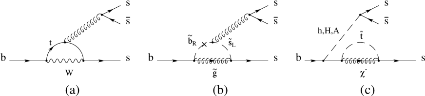
Figure 1: To illustrate different contributions, we show some Feynman diagrams relevant to $b\rightarrow ss\bar{s}$: (a) the SM, (b) the gluino mediated and (c) $\tan\beta-$enhanced Higgs mediated contributions.

Note that the gluino mediated QCD penguin operators are not enhanced in the large $\tan\beta$ region, unlike the Higgs-mediated contributions. But the gluino-mediated diagrams contribute to $b\rightarrow sq\bar{q}$ for all $q=u,d,s,c,b$, independent of flavor. Therefore one should check that these new sources of flavor changing do not contribute too much to other charmless $B$ decays such as $B\rightarrow\pi\pi,\pi K$, etc. In this paper we will not deal with this problem directly. But we note that there are known mechanisms by which this can be achieved. As an example, consider a scenario in which both $LL$ and $RR$ operators contribute to $B\to\phi K_{S}$ with nearly equal amplitudes. Because vector mesons ($\phi,\rho,\ldots$) and pseudoscalar mesons ($\pi,K,\eta^{(^{\prime})}$) have opposite parity, the gluino loop effects appear as $(\delta_{LL}^{d})_{23}+(\delta_{RR}^{d})_{23}$ for the $VP$ modes and $(\delta_{LL}^{d})_{23}-(\delta_{RR}^{d})_{23}$ for the $PP$ modes, respectively. So one can suppress the gluino contributions to the $PP$ modes by simply assuming $(\delta_{LL}^{d})_{23}=(\delta_{RR}^{d})_{23}$, even if $LL$ and $RR$ contributions are sizable kagan02 .

There are additional issues that arise in comparing $B\to\phi K_{S}$ to $B\to\pi\pi$ and others. For example, there are multiple diagrams contributing to processes such as $B\to\pi\pi$, unlike the case of $B\to\phi K_{S}$. This makes the inclusion of SUSY effects in these processes either irrelevant or highly uncertain. We will take an indirect approach to this problem by requiring that the total branching ratio of $B\to\phi K_{S}$ is consistent with observation after including SUSY effects. By demanding that the SUSY contributions to $B\to\phi K_{S}$ are of the same order or less than the SM contributions, we can safely assume that the SUSY contributions to related processes are also close to experiment. Given the uncertainties inherent in the BBNS or any other factorization scheme we feel that this is an appropriate approach. However it also means that the size of the strong phase will play an important role in our calculations, another reason for using the best technology available today, namely BBNS factorization.

The relevant Wilson coefficients due to the gluino box/penguin loop diagrams involving the $LL$ and $LR$ insertions are given (at the scale $\mu\sim m_{W}$) by ko01

$$C_{3}^{\rm SUSY} = -\frac{\alpha_{s}^{2}}{2\sqrt{2}G_{F}\widetilde{m}^{2}\lambda_{t}}\left(-\frac{1}{9}B_{1}(x)-\frac{5}{9}B_{2}(x)-\frac{1}{18}P_{1}(x)-\frac{1}{2}P_{2}(x)\right)\left(\delta^{d}_{LL}\right)_{23}$$

$$C_{4}^{\rm SUSY} = -\frac{\alpha_{s}^{2}}{2\sqrt{2}G_{F}\widetilde{m}^{2}\lambda_{t}}\left(-\frac{7}{3}B_{1}(x)+\frac{1}{3}B_{2}(x)+\frac{1}{6}P_{1}(x)+\frac{3}{2}P_{2}(x)\right)\left(\delta^{d}_{LL}\right)_{23}$$

$$C_{5}^{\rm SUSY} = -\frac{\alpha_{s}^{2}}{2\sqrt{2}G_{F}\widetilde{m}^{2}\lambda_{t}}\left(\frac{10}{9}B_{1}(x)+\frac{1}{18}B_{2}(x)-\frac{1}{18}P_{1}(x)-\frac{1}{2}P_{2}(x)\right)\left(\delta^{d}_{LL}\right)_{23}$$

$$C_{6}^{\rm SUSY} = -\frac{\alpha_{s}^{2}}{2\sqrt{2}G_{F}\widetilde{m}^{2}\lambda_{t}}\left(-\frac{2}{3}B_{1}(x)+\frac{7}{6}B_{2}(x)+\frac{1}{6}P_{1}(x)+\frac{3}{2}P_{2}(x)\right)\left(\delta^{d}_{LL}\right)_{23}$$

$$C_{7\gamma}^{\rm SUSY} = {8\pi\alpha_{s}\over 9\sqrt{2}G_{F}\tilde{m}^{2}\lambda_{t}}\left[(\delta_{LL}^{d})_{23}M_{4}(x)-(\delta_{LR}^{d})_{23}\left({m_{\tilde{g}}\over m_{b}}\right)4B_{1}(x)\right],$$

$$C_{8g}^{\rm SUSY} = -{2\pi\alpha_{s}\over\sqrt{2}G_{F}\tilde{m}^{2}\lambda_{t}}\left[(\delta_{LL}^{d})_{23}\left({3\over 2}M_{3}(x)-{1\over 6}M_{4}(x)\right)\right.$$ (10)

$$\left.+(\delta_{LR}^{d})_{23}\left({m_{\tilde{g}}\over m_{b}}\right)~{}{1\over 6}~{}\left(4B_{1}(x)-9x^{-1}B_{2}(x)\right)\right],$$

where $x\equiv(m_{\tilde{g}}/\tilde{m})^{2}$, and the loop functions can be found in Ref. ko01 . In the presence of the $RR$ and $RL$ insertions, we have additional operators $\widetilde{O}_{i=3\ldots 6,7\gamma,8g}$ that are obtained by $L\leftrightarrow R$ in the operators in the SM. The associated Wilson coefficients $\widetilde{C}_{i=3\ldots 6,7\gamma,8g}$ are given by the similar expressions as above with the replacement $L\leftrightarrow R$. The remaining coefficients are either dominated by their SM contributions ($C_{1,2}$) or are electroweak penguins ($C_{7\ldots 10}$) and therefore small.

A remark is in order concerning the above expressions. These Wilson coefficients differ from the 1996 results in Gabbiani et al. masiero96 in (i) the signs of the $(\delta_{LR}^{d})_{23}$ contributions in $C_{7\gamma}$ and $C_{8g}$, and (ii) the loop function $9xB_{2}(x)$ in $C_{8g}$ should be corrected to $9x^{-1}B_{2}(x)$ as given above . These differences are not important for numerical results, however.

The decay rate for $B\to\phi K_{S}$ is given by

$$\Gamma(B\to\phi K_{S})={G_{F}^{2}f_{\phi}^{2}m_{B}^{3}\over 32\pi}~{}(F_{1}^{B\rightarrow K})^{2}\left|a_{\phi K}^{\rm eff}\right|^{2}~{}\lambda^{3/2}(1,m_{\phi}^{2}/m_{B}^{2},m_{K}^{2}/m_{B}^{2})$$ (11)

where

$$a_{\phi K}^{\rm eff}=\sum_{p=u,c}\lambda_{p}\left[(a_{3}+a_{4}^{p}+a_{5})-{1\over 2}~{}(a_{7}+a_{9}+a_{10}^{p})\right]$$ (12)

and $\lambda$ is the magnitude of the $\phi$ 3-momentum relative to $m_{B}$. In the numerical analysis, we use $f_{\phi}=237$ MeV and $F_{1}^{B\rightarrow K}=0.38$. The $a_{i}$’s are given in terms of the Wilson coefficients $C_{i}$ times various nonperturbative hadronic parameters:

$$a_{3} = C_{3}+\frac{C_{4}}{N_{c}}+\frac{C_{4}}{N_{c}}\frac{C_{F}\alpha_{s}}{4\pi N_{c}}\left(N_{c}V_{\phi}+4\pi^{2}H_{\phi K}\right)$$

$$a_{4}^{p} = C_{4}+\frac{C_{3}}{N_{c}}+\frac{C_{3}}{N_{c}}\frac{C_{F}\alpha_{s}}{4\pi N_{c}}\left(N_{c}V_{\phi}+4\pi^{2}H_{\phi K}\right)+\frac{C_{F}\alpha_{s}}{4\pi}\frac{P^{p}_{\phi,2}}{N_{c}}$$

$$a_{5} = C_{5}+\frac{C_{6}}{N_{c}}-\frac{C_{6}}{N_{c}}\frac{C_{F}\alpha_{s}}{4\pi N_{c}}\left(N_{c}V^{\prime}_{\phi}+4\pi^{2}H^{\prime}_{\phi K}\right)$$

where $C_{F}=(N_{c}^{2}-1)/2N_{c}$ and $N_{c}=3$. The various $V^{(}{}^{\prime}{}^{)}$, $H^{(}{}^{\prime}{}^{)}$ and $P$ terms represent the nonperturbative hadronic parameters at the heart of the BBNS calculation and are described in Ref. bbns .

Besides generating the amplitudes necessary for calculating physical rates, the BBNS approach also provides us with the appropriate strong phase. We will digress for a moment to talk about the importance of this piece in the calculation.

In order to have nonzero CP asymmetries, we need at least two independent amplitudes with different weak and strong phases. In the SUSY models we are considering, the weak phases reside in the complex mass insertion parameters, the $\delta$’s, and appear in the Wilson coefficients $C_{3,...,6}$ and $C_{8g}$: see Fig. 1(a)–(c). These weak phases are odd under a CP transformation. On the other hand, the CP-even strong phases arise from scatterings among the final state particles. At the parton level, they are generated by gluon exchange between various quarks participating in the $B$ decay processes. In the BBNS approach there are four classes of diagrams that can generate strong phases: vertex corrections, penguins, hard scattering with spectators and annihilation diagrams. We show a vertex correction diagram in Fig. 2 for illustration, referring the reader to the BBNS papers bbns for the details. The strong phases are then encoded in the $V^{(}{}^{\prime}{}^{)}$, $H^{(}{}^{\prime}{}^{)}$ and $P$ terms that appear in the definitions of the $a_{i}$ parameters above.

Before the BBNS approach, the strong phase was generated by the so-called Bander-Soni-Silverman (BSS) mechanism, in which the one loop diagrams involving the 4-quark operators develop a strong phase consistent with unitarity. However, there is an ambiguity in this approach regarding the momentum flow into the quark loop, and one usually made the ad hoc assumption that the average $q^{2}$ through the virtual gluon is $\langle q^{2}\rangle\simeq m_{b}^{2}/4$. This ambiguity disappears in the BBNS approach, where one has a definite relation between the loop momenta of the quark and antiquark and the meson lightcone wavefunction. In particular, the contributions of the $b\rightarrow sg$ operators $O_{8g}$ and $\widetilde{O}_{8g}$ are obtained in an unambiguous way at least in the leading order.

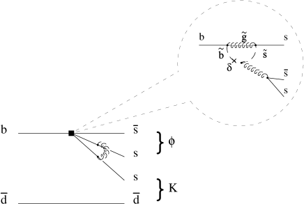
Figure 2: A typical final state interaction diagram which generates a strong phase in $B\to\phi K_{S}$. At long distances, the weak phase is contained in the 4-fermion vertex shown as a small square. At short distances, that vertex resolves to SUSY diagrams like those studied in this paper.

IV $B\to X_{s}\gamma$

It has long been claimed that the most stringent bounds on the $(\delta_{AB}^{d})_{23}$ insertion comes from $b\to s\gamma$ (or $B\rightarrow X_{s}\gamma$). Because the measured value is close to the SM prediction, there is little room for new physics lurking into $b\rightarrow s$ transition. This statement is particularly true for $LR$ mixing because the SUSY contributions interfere with the SM ones at the amplitude level (in $C_{7\gamma}$ and $C_{8g}$) and further because the SUSY contributions pick up an $m_{\widetilde{g}}/m_{b}$ enhancement relative to the SM. The $LL$ insertion also contributes to $C_{7\gamma,8g}$ but lacks the gluino mass enhancement. Thus $LL$ insertions can be very large while remaining consistent with $b\to s\gamma$, while $LR$ insertions are constrained to be small, of ${\cal O}(10^{-2})$.

The contribution of the $RL$ and $RR$ insertions to $C_{7\gamma,8g}$ are suppressed by $m_{s}/m_{b}$ where $m_{s}$ is the strange quark mass and so we ignore them. However they make unsuppressed contributions to $\widetilde{C}_{7\gamma,8g}$, but because these operators do not appear in the SM, their contributions cannot interfere with the SM, nor can they generate CP violation. Thus the constraint from $B\to X_{s}\gamma$ on $RL$ and $RR$ operators will always be somewhat weaker than that on $LR$ and $LL$ operators respectively.

We will impose a rather generous bound for $B\rightarrow X_{s}\gamma$,

$$2.0\times 10^{-4}<B(B\rightarrow X_{s}\gamma)<4.5\times 10^{-4},$$

in order to take into account the theoretical uncertainties in the NLO calculation of the SUSY contributions. (We have also checked that our results for $S_{\phi K}$ do not change very much if we narrow the allowed window for the $B\rightarrow X_{s}\gamma$ branching ratio. It will be relatively straightforward to see the effect of narrowing the window in the figures we present in Section VI.) The CP-averaged branching ratio for $B\rightarrow X_{s}\gamma$ in the leading log approximation is given by

$${B(B\rightarrow X_{s}\gamma)\over B(B\rightarrow X_{c}e\nu)}=\left|{V_{ts}^{*}V_{tb}\over V_{cb}}\right|^{2}~{}{6\alpha\over\pi f(z)}~{}\left[|C_{7\gamma}(m_{b})|^{2}+|\widetilde{C}_{7\gamma}(m_{b})|^{2}\right].$$ (13)

where $f(z)=1-8z+8z^{3}-z^{4}-12z^{2}\log z$ is the phase space factor for the $b\rightarrow c$ semileptonic decays and $\alpha^{-1}=137.036$. Neglecting the RG running between the heavy SUSY particles and the top quark mass scales, we get the following relations :

$$C_{7\gamma}(m_{b}) \simeq -0.31+0.67~{}C_{7\gamma}^{\rm SUSY}(m_{W})+0.09~{}C_{8g}^{\rm SUSY}(m_{W}),$$

$$C_{8g}(m_{b}) \simeq -0.15+0.70~{}C_{8g}^{\rm SUSY}(m_{W}).$$ (14)

In most of our analysis of $B\to X_{s}\gamma$ we will assume that the only contributions are those of the SM plus the gluino-mediated SUSY loops. It is well known that the charged Higgs and chargino sectors in the MSSM may contribute to $B\to X_{s}\gamma$ with strengths equal to or greater than the SM piece. We will ignore this possibility except in Section VI.3.1, where we will consider a particularly interesting limit in which all but the gluino loops cancel out among themselves.

A new CP-violating phase in $(\delta^{d}_{AB})_{23}$ will also generate CP violation in $B\rightarrow X_{s}\gamma$. In order to have a nonvanishing direct CP asymmetry, one needs at least two independent amplitudes with different strong (CP-even) and weak (CP-odd) phases. In $B\rightarrow X_{s}\gamma$, strong phases are provided by quark and gluon loop diagrams, whereas weak phases are provided by the CKM angles and $(\delta_{AB}^{d})_{23}$. For conventional models with the same operator basis as in the SM, the resulting direct CP asymmetry in $B\rightarrow X_{s}\gamma$ can be written as ali ; kn

$$A_{\rm CP}^{b\to s\gamma}({\rm in}~{}\%)={1\over|C_{7\gamma}|^{2}}~{}\left[1.23~{}{\rm Im}\left(C_{2}C_{7\gamma}^{*}\right)-9.52~{}{\rm Im}\left(C_{8g}C_{7\gamma}^{*}\right)+0.10~{}{\rm Im}\left(C_{2}C_{8g}^{*}\right)\right].$$ (15)

Since SUSY contributions to $C_{2}$ are negligible, we use $C_{2}(m_{b})\simeq C_{2}^{\rm SM}(m_{b})\simeq 1.11$. In the presence of operators $\widetilde{O}_{i}$ with opposite chirality, Eq. (15) is modified according to Ref. kn . Within the SM, the predicted CP asymmetry is less than $\sim 0.5\%$; any larger asymmetry would be a clear indication of new physics.

What we currently know about $A_{\rm CP}^{b\to s\gamma}$ comes from CLEO cleo :

$$A_{\rm CP}^{b\to s\gamma}=(-7.9\pm 10.8\pm 2.2)(1.0\pm 0.030)\%.$$ (16)

This is clearly not a very strong constraint at present, but should become significantly more important in the near future.

Despite the importance of $B\rightarrow X_{s}\gamma$ for constraining $(\delta_{AB}^{d})_{23}$, we will find in the following sections that the $B\rightarrow\phi K$ branching ratio itself provides a constraint on the $LR$ and $RL$ insertions which is every bit as strong as $B\rightarrow X_{s}\gamma$.

V $B_{s}^{0}$–$\bar{B}_{s}^{0}$ mixing

Gluino-mediated box diagrams will also affect $B_{s}^{0}$–$\bar{B}_{s}^{0}$ mixing, which is phenomenologically very important. The most general effective Hamiltonian for $B_{s}^{0}$–$\bar{B}_{s}^{0}$ mixing ($\Delta B=2$) and its SUSY contributions have been calculated in Refs. masiero2002 ; kkp and we do not repeat that discussion here. Following the explicit formulation of Ref. kkp , we calculate $\Delta M_{s}$ and the phase of the $B_{s}^{0}$–$\bar{B}_{s}^{0}$ mixing, $\beta_{s}$. For the $B_{d,s}$ meson decay constants, we have assumed $f_{B_{d}}=200\pm 30$ MeV, and

$${f_{B_{s}}^{2}B_{B_{s}}\over f_{B_{d}}^{2}B_{B_{d}}}=1.16\pm 0.05.$$

Currently, only the experimental lower limit $\Delta M_{B_{s}}>14.9~{}{\rm ps}^{-1}$ is known bs-exp . Also we assume that the SUSY effects on $B^{0}$–$\bar{B}^{0}$ mixing are reasonably small kkp (i.e., $\theta_{d}$ in Eq. 6 is nearly zero). According to the analysis by Ko et al. kkp , the CKM angle $\gamma$ can still be in the range between $-60^{\circ}$ and $60^{\circ}$ for the $LL$ insertion $(\delta_{LL}^{d})_{13}\neq 0$ without any conflict with the measured $\Delta M$ and $\sin 2\beta_{\psi K_{S}}$. Then these effects will only appear in $\lambda_{\phi K}$ as $2(\beta+\theta_{d})$, which is fixed to be $\sin 2\beta_{\psi K}=0.734\pm 0.054$ by data. Furthermore, the SM contributions to $B\to\phi K_{S}$ or $B_{s}^{0}$–$\bar{B}_{s}^{0}$ mixing are independent of the CKM angle $\gamma$, so that we don’t have to worry about the SUSY contribution to $B^{0}$–$\bar{B}^{0}$ mixing.

In our model, the CP violating phase in the mass insertion parameters $(\delta_{AB}^{d})_{23}$ contributes not only to $S_{\phi K}$, as discussed before, but also to the imaginary part of the $B_{s}^{0}$–$\bar{B}_{s}^{0}$ mixing, $M_{12}(B_{s})$, which is real within the SM to a very good approximation. Thus there should be some correlation between $S_{\phi K}$ and $2\beta_{s}\equiv-\mbox{Arg}\,[M_{12}(B_{s})]$. The observable $S_{\psi\phi}=\sin 2\beta_{s}$ plays the same role in $B_{s}\to\psi\phi$ as $S_{\phi K}$ does in $B\to\phi K_{S}$, and thus we may expect large deviations in the time-dependent decays of $B_{s}$ into $\psi\phi$. The SM predicts $\beta_{s}$ vanishes (to experimental accuracy), so any measurement of a non-zero $\beta_{s}$ would be a sign of new physics.

The new phase in $B_{s}^{0}$–$\bar{B}_{s}^{0}$ mixing will also appear in the dilepton charge asymmetry of $B$ decays that can be measured at hadron colliders (see, e.g., randall ):

$$A_{\ell\ell}\equiv\frac{N(\ell^{+}\ell^{+})-N(\ell^{-}\ell^{-})}{N(\ell^{+}\ell^{+})+N(\ell^{-}\ell^{-})}=\frac{N(BB)-N(\bar{B}\bar{B})}{N(BB)+N(\bar{B}\bar{B})}\simeq{\rm Im}(\Gamma_{12}/M_{12}).$$ (17)

In the SM, the phases of $M_{12}$ and $\Gamma_{12}$ are almost the same, and $A_{\ell\ell}^{\rm SM}\simeq 10^{-4}$ ($10^{-3}$ for $B_{d}$). But in the presence of SUSY, a much larger dilepton charge asymmetry may be possible. Though SUSY is not expected to provide a large correction to $\Gamma_{12}$ (which is dominated by large SM contributions), it can strongly affect $M_{12}$. In such a case, the dilepton charge asymmetry could be approximated as

$$A_{\ell\ell}\simeq{\rm Im}\left({\Gamma_{12}^{\rm SM}\over M_{12}^{\rm SM}+M_{12}^{\rm SUSY}}\right).$$ (18)

The possible range of $A_{\ell\ell}$ in a classes of SUSY models were studied in Refs. randall ; kkp . We will follow the formulation of Ref. kkp in our analysis. We will demand that all solutions obey the lower bound $\Delta M_{s}>14.9\,\mbox{ps}^{-1}$, and for those that do, present their prediction for $\Delta M_{s}$.

VI Numerical Analyses of Gluino Mediation

Now we come to the heart of our analysis. We would like to consider whether gluino-induced flavor changing can explain the $B\to\phi K_{S}$ data while remaining consistent with all other known constraints. And if so, we wish to identify other observables that can be used to check our interpretation of the data. We will consider each possible mass mixing $(\delta^{d}_{AB})_{23}$ for $AB=LL,LR,RL,RR$ one at a time. The technique assumes that only one insertion dominates the new physics. However, where relevant, we will explain how a second, subdominant insertion could change some of the correlating observables.

In all of the studies that follow, we will scan over the modulus and phase of the flavor-changing mass insertions ($|\mbox{Re,Im}\,(\delta^{d}_{AB})_{23}|\leq 1$), calculating all observables for a fixed gluino and (universal) squark mass of $400\,\mbox{GeV}$. We will then vary the ratio $x=m^{2}_{\widetilde{g}}/\widetilde{m}^{2}$ away from unity (keeping $m_{\widetilde{g}}$ fixed) and finally, at the end of the section, discuss the effects of varying the gluino mass. We will keep only those points which are consistent with the branching ratio for $B\to X_{s}\gamma$, and which have $\Delta M_{s}>14.9\,\mbox{ps}^{-1}$. Both of these constraints were discussed in previous sections. We will also require that the branching ratio for $B\to\phi K_{S}$ be less than $1.6\times 10^{-5}$, as calculated in the BBNS approach. This value is twice the observed branching ratio, but we feel that the uncertainties inherent in the BBNS factorization scheme may be large enough to merit this window.

VI.1 The $LL$ and $RR$ insertions

We will begin by considering the the $LL$ and $RR$ insertions, though assuming that one or the other appears dominantly. Since the physics effects of these two operators are almost identical, we will couch our discussion in the language of the $LL$ insertion and specifically point out those few places where the $RR$ analysis diverges.

A non-zero $LL$ mass insertion $(\delta_{LL}^{d})_{23}$ generates the QCD penguin operators $O_{3,...,6}$ and the (chromo)magnetic operators $O_{7\gamma,8g}$. The $B\to X_{s}\gamma$ and $\Delta M_{s}$ constraints remove two distinct regions in the $\{\mbox{Re}\,(\delta^{d}_{LL})_{23},\mbox{Im}\,(\delta^{d}_{LL})_{23}\}$ plane. The constraint on the branching ratio of $b\to s\gamma$ removes all points with $\mbox{Re}\,(\delta^{d}_{LL})_{23}<-0.5$. The constraint that $\Delta M_{s}>14.9\,\mbox{ps}^{-1}$ removes points where $|\mbox{Re}\,(\delta^{d}_{LL})_{23}|<0.25$ and $0.25<|\mbox{Im}\,(\delta^{d}_{LL})_{23}|<0.75$. See Fig. 3(a). The resulting $\Delta M_{s}$ is indicated by the different colors. For $x=1$, $\Delta M_{s}$ can be as large as $\sim 100$ ps^-1.

However, nowhere in the plane are we able to get substantial shifts in $S_{\phi K}$. In particular, for $m_{\widetilde{g}}=\widetilde{m}=400\,\mbox{GeV}$ we find no points with $S_{\phi K}<0.5$. (We will comment shortly about the effect of changing the SUSY masses.) The lack of impact on $S_{\phi K}$ arises in part because of substantial cancellations between $C_{3\dots 6}^{\rm SUSY}$ and $C_{8g}^{\rm SUSY}$. This result is consistent with that obtained by Lunghi and Wyler lunghi . If we lower the common squark mass to $x=3$, the asymmetries become somewhat smaller and $\Delta M_{s}$ can be as large as a few tens of ps^-1. On the other hand, for a heavier squark of $x=0.5$, $\Delta M_{s}$ can be even larger than 100 ps^-1, which is beyond the reach of hadron colliders.

(On the other hand, if we lower the gluino mass down to $250$ GeV with $x=1$, $S_{\phi K}$ can shift down as low as $0.05$, but this is possible only if the gluino and squark masses are close their current lower limits of 200 to $250\,\mbox{GeV}$. See the Section VI.4 for further discussion.)

Furthermore there is very little effect on $C_{\phi K}$ and $A_{\rm CP}^{b\to s\gamma}$, the former varying only between $\pm 0.1$, the latter between $\pm 3\%$ (see the figure). However there are one-to-one correlations among $S_{\phi K}$, $C_{\phi K}$ and $A_{\rm CP}^{b\to s\gamma}$ for an $LL$ insertion, so measuring these correlations would provide strong evidence for the model. However the experimental precision achievable in the near future will make this a very difficult task.

The lack of signal in $B\to\phi K_{S}$ and $B\to X_{s}\gamma$ does not mean that an $LL$ insertion is without signature. It is clear from Fig. 3(e) that there can be sizable effects in the dilepton charge asymmetry $A_{\ell\ell}$, with asymmetries as large as an order of magnitude above the SM. But the largest effect is in the $B_{s}$ sector, specifically $B_{s}^{0}$–$\bar{B}_{s}^{0}$ mixing and the CP-violating phase $\beta_{s}$ measured in $B_{s}\to\psi\phi$. Examining Figs. 3(a),(e) and (f), it is remarkable that SUSY could drive $\Delta M_{s}$ to values as large as $100\,\mbox{ps}^{-1}$, and could shift the CP asymmetry to any value $|\sin 2\beta_{s}|\leq 1$. Thus an $LL$ insertion may be better probed in $B_{s}$ decays than in $B_{d}$ decays such as $B\to\phi K_{S}$.

In summary we conclude that the effects of the $LL$ insertion on $B\to\phi K_{S}$ are insignificant unless the squarks and gluino are very close to their current experimental limit. For squarks and gluinos with masses of several hundred GeV or more, the $LL$ insertion alone is inadequate for explaining the current data on $S_{\phi K}$. However, the $LL$ insertion plays its strongest role in the $B_{s}$ system, where it can contribute sizably to $B_{s}^{0}$–$\bar{B}_{s}^{0}$ mixing even for heavy squarks and gluinos. Thus there remains the possibility that $\Delta M_{s}$ and $\sin 2\beta_{s}$ will be quite large while $B\to\phi K_{S}$ and $B\to X_{s}\gamma$ remain close to their SM predictions.

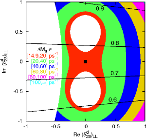
(a) Allowed region for the $LL$ insertion

(b) $S_{\phi K}$ vs. $B(B\to\phi K_{S})$

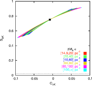
(c) $S_{\phi K}$ vs. $C_{\phi K}$

(d) $S_{\phi K}$ vs. $A_{\rm CP}^{b\to s\gamma}$

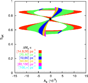
(e) $S_{\phi K}$ vs. $A_{\ell\ell}$

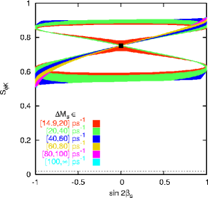
(f) $S_{\phi K}$ vs. $\sin 2\beta_{s}$

Figure 3: (a) The allowed region in the $({\rm Re}\,(\delta_{LL}^{d})_{23},{\rm Im}\,(\delta_{LL}^{d})_{23})$ plane, and the correlations between (b) $S_{\phi K}$ and $B(B\to\phi K_{S})$, (c) $S_{\phi K}$ and $C_{\phi K}$, (d) $S_{\phi K}$ and $A_{\rm CP}^{b\to s\gamma}$, (e) $S_{\phi K}$ and $A_{\ell\ell}$, and (f) $S_{\phi K}$ and $\sin 2\beta_{s}$ for $m_{\tilde{g}}=400$ GeV and $x=1$. Different shades are used for different ranges of $\Delta M_{s}$. The small black boxes represent the SM prediction.

The physics of the $RR$ insertion is identical in almost every way to that of the $LL$ insertion. The prime exception is the $b\to s\gamma$ constraint, which is weaker because the $RR$ contribution does not interfere with the dominant SM amplitude for $B\to X_{s}\gamma$.

Therefore, the entire region of $\{\mbox{Re}\,(\delta_{RR}^{d})_{23},\mbox{Im}\,(\delta_{RR}^{d})_{23}\}$ with $|(\delta_{RR}^{d})_{23}|\leq 1$ is now allowed apart from the small areas in which $\Delta M_{s}<14.9\,\mbox{ps}^{-1}$: see Fig. 4(a). In Fig. 4, we show the plots for the $RR$ insertion case with $m_{\tilde{g}}=\tilde{m}=400$ GeV. It is obvious that the $RR$ case is essentially identical to the $LL$ case in Fig. 3. There are two issues which are not obvious from the figures. First, as already indicated, the $RR$ insertion contributes very little to $B\to X_{s}\gamma$. Thus we have omitted a plot of the prediction of the direct CP violation in $B\to X_{s}\gamma$, $A_{\rm CP}^{b\to s\gamma}$, since it would differ little from the SM. Secondly, for light gluinos and squarks, near their experimental limit, it is possible to get slightly lower values of $S_{\phi K}$ for the $RR$ insertion than it was for the $LL$; this is because the $LL$ insertions required to further push down $S_{\phi K}$ are inconsistent with $B\to X_{s}\gamma$.

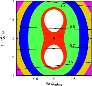
(a) Allowed region for the $RR$ insertion

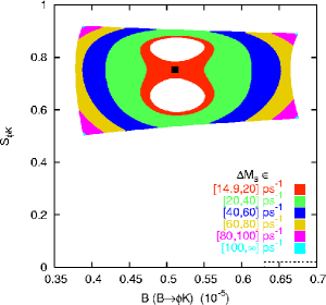
(b) $S_{\phi K}$ vs. $B(B\to\phi K_{S})$

(c) $S_{\phi K}$ vs. $C_{\phi K}$

(d) $S_{\phi K}$ vs. $\sin 2\beta_{s}$

Figure 4: (a) The allowed region in the $({\rm Re}\,(\delta_{RR}^{d})_{23},{\rm Im}\,(\delta_{RR}^{d})_{23})$ plane, and the correlations between (b) $S_{\phi K}$ and $B(B\to\phi K_{S})$, (c) $S_{\phi K}$ and $C_{\phi K}$, (d) $S_{\phi K}$ and $\sin 2\beta_{s}$ for $m_{\tilde{g}}=400$ GeV and $x=1$. Different shades are used for different ranges of $\Delta M_{s}$.

A few general remarks on the $LL$ and $RR$ insertions are in order. First, we note that one requires a large 2-3 mixing in order to obtain any observable effect in $S_{\phi K}$. But for such large mixing, our mass insertion approximation is no longer valid. One must then consider the full vertex mixings in the $d_{i}-\tilde{d}_{j}-\tilde{g}$ couplings with squarks in the mass eigenstates, as done in Ref. murayama . In this case, the superGIM suppression is less effective and the loop functions are enhanced, which could lead to somewhat larger effects on $B\to\phi K_{S}$.

If one considers a large 2-3 mixing in the $LL$ or $RR$ sector, an important constraint from $B^{0}$–$\bar{B}^{0}$ mixing, which is proportional to $(\delta_{AB}^{d})_{13}$, may also arise. Since the SM contribution to $\Delta M_{d}$ is proportional to $(V_{tb}V_{td}^{*})^{2}$, the gluino loop contribution with light gluinos/squarks can easily dominate the SM, unless the $RR$ or $LL$ insertion for $b\rightarrow d$ transition is very small. In Ref. kkp , two of us discussed the allowed region for the $(\delta_{LL}^{d})_{13}$ insertion, imposing the measured $\Delta M_{d}$, $\sin 2\beta_{\psi K}$ and $B\rightarrow X_{d}\gamma$. It was found that one needs $(\delta_{LL}^{d})_{13}\lesssim 5\times 10^{-2}$ even if we assume that the CKM angle $\gamma$ is a completely free parameter. This should be compared to $(\delta_{LL}^{d})_{23}\sim 1$ which is needed in order for the $LL$ insertion to explain the observed shift in $S_{\phi K}$. It would be difficult, although not impossible, to build a flavor model where this is the case.

VI.2 The $LR$ insertion

The case of an $LR$ insertion of the form $\widetilde{s}_{L}^{\dagger}\widetilde{b}_{R}$ is very different from that of either $LL$ or $RR$. While $LL$, $RR$ insertions can be ${\cal O}(1)$, the parameters $(\delta_{AB}^{d})_{23}$’s must be small in order to avoid excessively large FCNC amplitudes in charmless nonleptonic $B$ decays. But this also implies that even small $(\delta_{AB}^{d})_{23}$’s can lead to observable effects in the $B$ sector. The analysis of the $LR$ insertion is particularly simple, in part because it does not contribute to the penguin operators $C_{3\ldots 10}$. But its contributions to the (chromo)magnetic dipole operators can be quite large because it breaks the SM chiral symmetry in the $b$-quark sector allowing dipole operators to occur without the usual $m_{b}$ suppression, replaced instead with a SUSY-breaking $m_{\widetilde{g}}$ insertion. Thus, as previously noted, the $LR$ insertion is much more strongly constrained by $B\rightarrow X_{s}\gamma$, roughly $|(\delta_{LR}^{d})_{23}|\lesssim 10^{-2}$. However the same chiral symmetry breaking also ensures that the $LR$ contributions to $C_{8g}$ are likewise large, and so there may still be a residual effect on $B\to\phi K_{S}$, both in its branching ratio and CP asymmetries. (This last effect was also noticed in Refs. kagan ; kagan02 ).

In Fig. 5(a), the allowed region for $\{{\rm Re}(\delta_{LR}^{d})_{23},{\rm Im}(\delta_{LR}^{d})_{23}\}$ is shown for $\tilde{m}=400\,\mbox{GeV}$ and $x=1$. The dark regions are consistent with the $B(B\to X_{s}\gamma)$ and $\Delta M_{s}$ constraints, but are not constrained by the bound on the $B\to\phi K_{S}$ branching ratio. We impose this constraint by hatching the regions in which $B(B\to\phi K_{S})>1.6\times 10^{-5}$. Note that there are large regions of parameter space which are consistent with $b\to s\gamma$ but not $B(B\to\phi K_{S})$, as we advertised. And though $(\delta^{d}_{LR})_{23}$ is constrained to be $\lesssim 10^{-2}$, it is still very important for $B\to\phi K_{S}$, affecting both its branching ratio and the asymmetries $S_{\phi K}$ and $C_{\phi K}$ by significant amounts. In particular, it is encouraging that the branching ratio for $B\to\phi K_{S}$ can easily be enhanced compared to the SM, moving it closer to the experimental data.

(a) Allowed region for the $LR$ insertion

(b) $S_{\phi K}$ vs. $B(B\to\phi K_{S})$

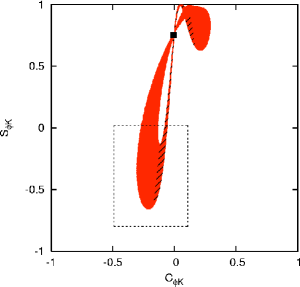
(c) $S_{\phi K}$ vs. $C_{\phi K}$

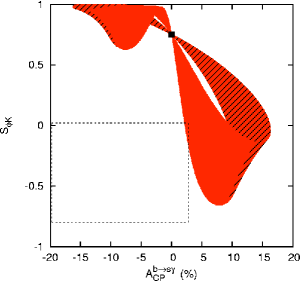
(d) $S_{\phi K}$ vs. $A_{\rm CP}^{b\to s\gamma}$

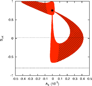
(e) $S_{\phi K}$ vs. $A_{\ell\ell}$

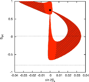
(f) $S_{\phi K}$ vs. $\sin 2\beta_{s}$

Figure 5: (a) The allowed region in the $({\rm Re}\,(\delta_{LR}^{d})_{23},{\rm Im}\,(\delta_{LR}^{d})_{23})$ plane, and the correlations between (b) $S_{\phi K}$ and $B(B\to\phi K_{S})$, (c) $S_{\phi K}$ and $C_{\phi K}$, (d) $S_{\phi K}$ and $A_{\rm CP}^{b\to s\gamma}$, (e) $S_{\phi K}$ and $A_{\ell\ell}$, and (f) $S_{\phi K}$ and $\sin 2\beta_{s}$ in the $LR$ insertion case for $m_{\tilde{g}}=400$ GeV and $x=1$. The dotted boxes show the $1\,\sigma$ current expermental data, and the hatched regions represent the region where $B(B\to\phi K_{S})>1.6\times 10^{-5}$.

Fig. 5(b) indicates that the branching ratio for $B\to\phi K_{S}$ can in fact be greatly enhanced relative to the SM case. Also note that $S_{\phi K}$ can take any value between $-0.6$ and 1, even after we impose $B(B\to\phi K_{S})<16\times 10^{-6}$ as a constraint. This is because the SUSY amplitude has a size similar to the SM amplitude so that the resulting branching ratio is not too different from the SM prediction. But it has very different strong and weak phases from the SM amplitude so that $S_{\phi K}$ and $C_{\phi K}$ can vary greatly with respect to SM predictions.

In Fig. 5(c), we show the correlation between $S_{\phi K}$ and $C_{\phi K}$. Note that we can get negative $S_{\phi K}$, for which $C_{\phi K}$ also becomes negative. Conversely, a positive $C_{\phi K}$ implies that $S_{\phi K}>0.6$ in our model. Thus the current data on $S_{\phi K}$ argues strongly in favor of a negative $C_{\phi K}$ if the $LR$ insertion is dominating the new physics contributions. This correlation between $S_{\phi K}$ and $C_{\phi K}$ will be tested at B factories in the near future.

The correlation between $S_{\phi K}$ and the direct CP asymmetry in $B\rightarrow X_{s}\gamma$ ($\equiv A_{\rm CP}^{b\to s\gamma}$) is shown in Fig. 5(d). We find $A_{\rm CP}^{b\to s\gamma}$ becomes positive for a negative $S_{\phi K}$, and a negative $A_{\rm CP}^{b\to s\gamma}$ implies that $S_{\phi K}>0.6$. However the present CLEO bound on $A_{\rm CP}^{b\to s\gamma}$ (Eq. 16) cannot constrain the $LR$ model very much.

In Fig. 5(e), the correlation between $S_{\phi K}$ and $A_{\ell\ell}$ is shown. Note that $A_{\ell\ell}\sim 10^{-4}$ within the SM so that any appreciable amount of $A_{\ell\ell}$ will be a clear indication of new physics in $B_{s}^{0}$–$\bar{B}_{s}^{0}$ mixing. For our model with the $LR$ insertion, the deviation of $A_{\ell\ell}$ from the SM prediction is small after imposing the $B\rightarrow X_{s}\gamma$ and $B\to\phi K_{S}$ branching ratio constraints. Finally in Fig. 5(f), we show the correlation between $S_{\phi K}$ and $\sin 2\beta_{s}$ (the latter of which is zero within the SM). Note that $\sin 2\beta_{s}$ is nothing but $S_{\psi\phi}$ in the $B_{s}\to\psi\phi$ decay, and can be measured at hadron colliders if $\Delta M_{s}$ is not too large. However, the resulting $\sin 2\beta_{s}$ for an $LR$ insertion is too small to be observed.

If we lower the common squark mass to $x=3$ for a fixed $m_{\widetilde{g}}=400\,\mbox{GeV}$, the asymmetries become somewhat smaller and $\Delta M_{s}$ can be in the range $[15.8,16.2]$ ps^-1. On the other hand, for a heavier squark $x=0.5$, the asymmetries can be larger, but we still have $\Delta M_{s}\simeq\Delta M_{s}^{\rm SM}$. Thus the results are not particularly sensitive to the gluino and squark masses. As the masses get very large the SUSY contributions slowly decreases, and are too small to provide an explanation for a negative $S_{\phi K}$.

Before closing this subsection, let us comment further on the sensitivity of our results to the methods used for calculating the hadronic amplitude. It is clear that the direct CP asymmetry $C_{\phi K}$ depends very strongly on the method used for evaluating hadronic matrix elements. For example, one finds $C_{\phi K}=0$ in naive factorization (without one loop corrections to the matrix elements of four-quark operators), whereas it can take on values of ${\cal O}(1)$ in the BBNS approach. The calculation of $S_{\phi K}$ is also technique-dependent, though less so. Different calculation schemes can produce values of $S_{\phi K}$ which are different by factors of a few. For example, $S_{\phi K}$ can go as negative as $-0.6$ in the $LR$ insertion case when we use the recent BBNS approach, but when the same parameter space is studied using the techniques of Lunghi and Wyler lunghi , $S_{\phi K}$ only drops as negative as $-0.2$. We consider the BBNS approach to be the most accurate and well-motivated available, which is why we use it, but view the differences between these schemes to be an unavoidable source of uncertainty at present.

VI.3 The $RL$ insertion

The final case to be considered is perhaps the most unusual. An $RL$ insertion is of the form $\widetilde{s}_{R}^{\dagger}\widetilde{b}_{L}$, coupling the RH strange squark to the LH bottom squark. Our intuition from the SM would lead us to believe that such insertions would be small compared to $LR$ insertions, naturally suppressed by $\sim m_{s}/m_{b}$. In SUSY models with minimal flavor violation, this is indeed the case. However, once one moves beyond minimal flavor violation there is no reason for the $RL$ insertion to be particularly suppressed with respect to $LR$. Furthermore, it has a phenomenology that is quite different than the $LR$ insertions because it does not interfere with the SM contributions which are themselves of the $LR$ form. (Because of this, we had to extend the BBNS approach to the case with opposite chirality 4-quark operators.) A quick comparison of the results for the $RL$ insertion in Fig. 6 to those of the $LR$ in the last section should convince the reader of this easily.

Though the $RL$ insertion generates a wide range in $B(B\to\phi K_{S})$ like the $LR$ case (Fig. 6(b)), the similarities end there. Because the $RL$ insertions do not directly interfere with the SM, the allowed region for $(\delta^{d}_{23})_{RL}$ is centered around zero (that is, only its square is relevant in most observables) as seen in Fig. 6(a). And although both cases can easily generate large, negative $S_{\phi K}$ and negative $C_{\phi K}$, only in the $LR$ case is the correlation completely clean. As we pointed in the previous section, an $LR$ insertion with negative $S_{\phi K}$ implies negative (but not very large) $C_{\phi K}$. For the $RL$ case, negative $S_{\phi K}$ can be accompanied by $C_{\phi K}$ of either sign (Fig. 6(c)). However there is a considerable hole in the figure around $C_{\phi K}=0$, which may help in disentangling the structure of the insertions once more data is to be had.

Otherwise $RL$ insertions leave very little other evidence. They do not appreciably alter $\Delta M_{s}$, and they do not generate observable $A_{\rm CP}^{b\to s\gamma}$ or $A_{\ell\ell}$. Thus for a pure $RL$ insertion, one expects to reproduce the SM in almost all ways except in $B\to\phi K_{S}$. In fact, of all the cases we have considered so far, the $RL$ case best fits the current data, for precisely this reason.

There is a particularly interesting variation on the $RL$ theme that we now turn our attention towards.

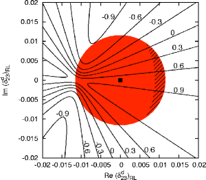
(a) Allowed region for the $RL$ insertion

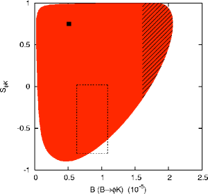
(b) $S_{\phi K}$ vs. $B(B\to\phi K_{S})$

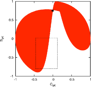
(c) $S_{\phi K}$ vs. $C_{\phi K}$

Figure 6: (a) The allowed region in the $(\mbox{Re}\,(\delta_{RL}^{d})_{23},{\rm Im}\,(\delta_{RL}^{d})_{23})$ plane, and the correlations between (b) $S_{\phi K}$ and $B(B\to\phi K_{S})$, (c) $S_{\phi K}$ and $C_{\phi K}$, and (d) $S_{\phi K}$ and $\Delta M_{s}$ for $m_{\tilde{g}}=400$ GeV and $x=1$. Current data at $1\,\sigma$ level is shown by the dotted boxes, and the hatched regions represent the region where $B(B\to\phi K_{S})>1.6\times 10^{-5}$.

VI.3.1 A special case: the $RL$ dominance scenario

Thus far, in our calculations of $B\to X_{s}\gamma$ we have made a simplifying assumption that can often be incorrect in realistic models. We have assumed that the calculation of $B\to X_{s}\gamma$ consists entirely of a SM piece and gluino-induced SUSY pieces. However low-energy models of SUSY usually have several other, often large, contributions to $B\to X_{s}\gamma$, most particularly from charged Higgs loops (which add to the SM terms), and from chargino loops (which subtract from the SM). It is well-known (see, e.g., Ref. bg ) that in the supersymmetric limit, the SM, charged Higgs and chargino contributions cancel each other exactly, predicting a rate for $B\to X_{s}\gamma$ of precisely zero. If SUSY is broken but the superpartners are relatively light, much of that cancellation can still occur. In such a case, the observed rate for $b\to s\gamma$ would be due almost entirely to the gluino loops.

Ref. kane has argued for just such an unconventional interpretation of $B\rightarrow X_{s}\gamma$. Here the Standard Model and usual SUSY contributions to $C_{7\gamma}$ approximately cancel: $C_{7\gamma}(m_{b})\approx C_{8g}(m_{b})\approx 0$. Then the dominant contribution to $b\to s\gamma$ is from the gluino-$\tilde{b}_{L}$-$\tilde{s}_{R}$ penguin in $\widetilde{C}_{7}$, and is proportional to $(\delta^{d}_{RL})_{23}$. We will call this the $RL$-dominance scenario in $b\to s\gamma$.

Now the constraint from $B\rightarrow X_{s}\gamma$ plays a completely different role in constraining our parameter space. Rather than limiting the size of the $RL$ insertion to be close to zero, it actually demands a finite non-zero value for the insertion in order to reproduce the observer branching ratio. Thus, it has the effect of constraining the complex parameter $(\delta_{RL}^{d})_{23}$ to lie in an annulus, just as the constraint from the $B\to\phi K_{S}$ branching fraction does (though of different center and radius). The resulting allowed parameter space is shown in Fig. 7(a) for $m_{\tilde{g}}=\tilde{m}=400$ GeV ($x=1$). In Fig. 7(b) and (c), we show the correlation of $S_{\phi K}$ with $B(B\to\phi K_{S})$ and $C_{\phi K}$, respectively. Note that $S_{\phi K}$ can take almost any value between $-1$ and $+1$ without conflict with the observed branching ratio for $B\to\phi K_{S}$. Also $C_{\phi K}$ can be positive for a negative $S_{\phi K}$, unlike the $LR$ case. In particular, $|C_{\phi K}|>0.2$ for $S_{\phi K}<0$. This could be a useful probe for identifying this scenario. Since there is only one diagram contributing to $b\to s\gamma$ in this scenario, one has $A_{\rm CP}^{b\to s\gamma}=0$ trivially.

However, as discussed in Ref. kane , if $(\delta_{RR}^{d})_{23}$ is also nonzero then $A_{\rm CP}^{b\to s\gamma}$ arises as an interference between $\widetilde{C}_{7\gamma}$ and $\widetilde{C}_{8g}$. Then the $RR$ insertion can contribute more significantly to $\Delta M_{s}$; we will not study this more complicated scenario here because the observables will depend crucially on the relative size of the various insertions. For example, the $RL$ insertion could be induced by a large $LL$ or $RR$ insertion coupled with an extra SU(2)-violating mass insertion. In such a case, there could be large deviations both in $S_{\phi K}$ and $B_{s}^{0}$–$\bar{B}_{s}^{0}$ mixing. Nonetheless, the correlations between $S_{\phi K}$ and $C_{\phi K}$ that we demonstrate in this paper depend primarily on the $LR$ or $RL$ insertions, and thus are good probes of new physics contributions to $B\to\phi K_{S}$.

Finally in the allowed region of $(\delta_{RL}^{d})_{23}$, we find $\Delta M_{s}<16.5$ ps^-1, whereas the SM prediction is $\Delta M_{s}=16.2$ ps^-1. If the pure $RL$-dominance scenario is realized in nature, $B_{s}^{0}$–$\bar{B}_{s}^{0}$ mixing will be observed shortly at the Tevatron. On the other hand, both $A_{\ell\ell}$ and $\sin 2\beta_{s}$ are too small to be observed.

If we lower the common squark mass to $x=3$, the asymmetries become somewhat smaller and $\Delta M_{s}$ falls in the range $[15.7,16.7]$ ps^-1. On the other hand, for a heavier squark $x=0.5$, the asymmetries can be larger, but $\Delta M_{s}\simeq\Delta M_{s}^{\rm SM}$.

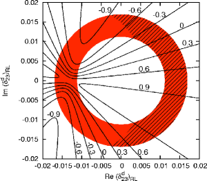
(a) Allowed region for the $RL$ insertion

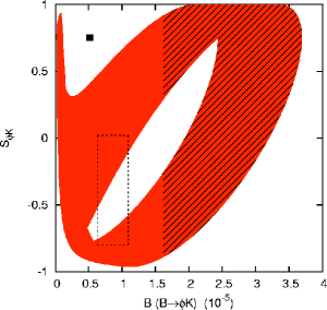
(b) $S_{\phi K}$ vs. $B(B\to\phi K_{S})$

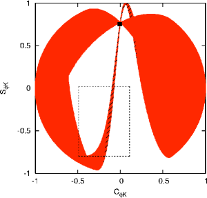
(c) $S_{\phi K}$ vs. $C_{\phi K}$

Figure 7: (a) The allowed region in the $({\rm Re}\,(\delta_{RL}^{d})_{23},{\rm Im}\,(\delta_{RL}^{d})_{23})$ plane in the special case of section VI.3.1, and the correlations between (b) $S_{\phi K}$ and $B(B\to\phi K_{S})$, (c) $S_{\phi K}$ and $C_{\phi K}$, and (d) $S_{\phi K}$ and $\Delta M_{s}$ for $m_{\tilde{g}}=400$ GeV and $x=1$. Current data at $1\,\sigma$ level is shown by the dotted boxes, and the hatched regions represent the region where $B(B\to\phi K_{S})>1.6\times 10^{-5}$.

In summary, $LR$ and $RL$ insertions of a size $\sim 10^{-3}$ – $10^{-2}$ can induce large shifts in $S_{\phi K}$ and $C_{\phi K}$ (and $A_{\rm CP}^{b\to s\gamma}$ for $LR$ insertion or for $RL+RR$ insertion) but will not affect $B_{s}^{0}$–$\bar{B}_{s}^{0}$ mixing, whereas the $LL$ and $RR$ insertions with a size $>0.2$ can induce large changes in $B_{s}^{0}$–$\bar{B}_{s}^{0}$ mixing (both in its modulus and phase) but are still too small in generic models to affect $S_{\phi K}$, $C_{\phi K}$ and $A_{\rm CP}^{b\to s\gamma}$ significantly. By understanding how each mass insertion individually affects the various observables, it is rather straightforward to go from here to the case in which more than one insertion is present. We will not complete that study here. However there has been recent work that benefits from multiple insertions that arise in well-motivated ultraviolet physics scenarios murayama , and we refer the reader there for further details.

VI.4 Gluino mass dependence of $S_{\phi K}$

In order to generalize our results and present a more complete picture of SUSY contributions in $B\to\phi K_{S}$, it is necessary to study how $S_{\phi K}$ changes as a function of the SUSY mass scale. We have already considered how changes in the squark mass scale, with the gluino scale held constant, will affect the observables. Now we turn to the gluino mass.

In particular, we have calculated $S_{\phi K}$ as a function of the gluino mass, for $x=1$, in each of the four insertion scenarios: $LL$, $RR$, $LR$ and $RL$. We have shown the results of our calculations in Fig. 8. In each of the four figures we have shaded in the allowed region of $S_{\phi K}$ as a function of $m_{\widetilde{g}}$. The different shades represent different predictions for $\Delta M_{s}$ as described in the figure legends. It is clear that $S_{\phi K}$ can have a large negative value very easily for the $LR$ or $RL$ insertion cases over a wide range of gluino and squark masses. On the other hand, in the $LL$ or $RR$ case $S_{\phi K}$ can have a large negative value only for a very light gluino (close to the current bound), and quickly reduces to the SM prediction as the gluino mass increases above $\sim 300$ GeV. For heavier squarks $x=0.5$, the window for a negative $S_{\phi K}$ increases slightly, but again the effect goes away quickly as $m_{\tilde{g}}$ becomes larger than $300\,\mbox{GeV}$. Furthermore, this always accompanies a very large $\Delta M_{s}$ (greater than 100 ps^-1). Thus Run II can rule out an $RR/LL$ explanation for $S_{\phi K}$ if gluinos are not found and/or $\Delta M_{s}<100\,\mbox{ps}^{-1}$ is measured.

These results speak directly to the analyses found in Refs. murayama ; masiero02 . Both of these analyses followed the same general lines as ours, but found that $RR$ insertions could sizably alter $S_{\phi K}$. The reasoning behind these claims is now clear. $RR$ insertions (and also $LL$ to a lesser extent) can indeed produce $S_{\phi K}<0$, but only for very light sparticles. Specifically, we find that $m_{\tilde{g}}$ must fall below $300\,\mbox{GeV}$ in order to obtain $S_{\phi K}<0$ with an $RR$ or $LL$ insertion. Like us, the authors of Ref. murayama find that large changes in $S_{\phi K}$ must be accompanied by large shifts in $\Delta M_{s}$, making it unobservable at the Tevatron. Ref. masiero02 disagrees with this finding, though the reasons probably have something to do with each groups’ estimations of the uncertainties in the BBNS factorization procedure. (See Section VI.5 for more discussion of this point.)

One note of explanation is needed in order to understand the graphs, and in particular why the $LR$ and $RL$ insertions seem to show no sign of decoupling, while decoupling is readily apparent for the $RR$ and $LL$ insertions. The reasoning quite simple. For the $RL$ and $LR$ insertions, the leading constraint comes from $B\to X_{s}\gamma$, which decouples at the same rate as the new physics contributions to $S_{\phi K}$. Thus, as $m_{\widetilde{g}}$ increases, the strength of the $B\to X_{s}\gamma$ constraint decreases, but the ratio of $(\delta_{LR,RL}^{d})_{23}/m_{\widetilde{g}}$ remains constant. On the other hand, there are no strong constraints on the $LL$ and $RR$ insertions, so even for light gluinos we have allowed values of $(\delta_{LL,RR}^{d})_{23}$ as large as 1; as the gluino mass increases, we are not free to increase the insertion any further to offset the mass suppression. Thus the effects on $S_{\phi K}$ fall as $1/m_{\widetilde{g}}^{2}$.

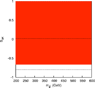
(a) $LR$ insertion

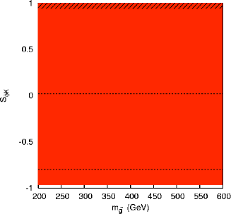
(b) $RL$ insertion

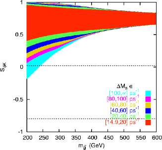
(c) $LL$ insertion

(d) $RR$ insertion

Figure 8: $S_{\phi K}$ as a function of $m_{\tilde{g}}$ for $x=1$. The shading represents $\Delta M_{s}$ in the ranges [14.9,20], [20,40], [40,60], [60,80], [80,100] and [100,$\infty$] ps^-1, respectively.

VI.5 Hadronic uncertainties

Finally, we should address the hadronic uncertainties within the BBNS approach to factorization. These uncertainties appear to be the origin of the qualitative differences that are found between our results in the previous subsections and those in Ref. masiero02 .

BBNS factorization fails two possibly important ways: it does not properly account for the subleading power corrections coming from annihilation diagrams, nor for those coming from hard scattering with a spectator quark. Each of these contributions should be subleading, but each involves an integral that blows up in the deep infrared (i.e., $\int_{0}^{1}dy/y$). Thus these “subleading” corrections are effectively infinite. In order to control the size of the integral, it is necessary to cut it off. We follow the original work of BBNS in parametrizing the integrals as $\Delta\equiv(1+\rho e^{i\varphi})\log(m_{B}/\lambda_{h})$ where $\lambda_{h}=500\,$MeV. For the results we have presented in this paper, we have taken $\Delta=0$; that is, we have assumed that the subleading corrections are very small.

However, we now wish to see how our results depend on the size and phase of $\Delta_{\rm hard}$ and $\Delta_{\rm annih}$. Again following BBNS, we vary $\rho$ and $\varphi$ in the ranges $0\leq\rho\leq 1$ and $0\leq\varphi\leq 2\pi$. (Each $\Delta_{\rm hard,annih}$ has its own $\rho,\varphi$ which are varied independently.) In Fig. 9 we consider the $RR$ insertion, since most recent works have emphasized this. For this case, the most negative value of $S_{\phi K}$ occurs at $(\delta^{d}_{23})_{RR}=1-i$, for fixed $m_{\tilde{g}}=250$ GeV and $x=1$. With this value of $(\delta^{d}_{23})_{RR}$, we plot $S_{\phi K}$ as a function of $m_{\tilde{g}}$. In Fig. 9(a), who show the result without the subleading corrections. In (b), we turn on the hard scattering corrections only; in (c) we do likewise for the annihilations corrections. Finally in (d) we allow both $\Delta_{\rm hard}$ and $\Delta_{\rm annih}$ to vary over their entire “allowed” ranges. Note that the annihilation diagrams generate much larger hadronic uncertainties than do the hard scattering amplitudes. Theoretical uncertainties decrease quickly for heavier gluinos, and there is no possibility to get a negative $S_{\phi K}$ for $m_{\tilde{g}}=\tilde{m}=400\,$GeV within the mass insertion approximation.

In the work of Ref. masiero02 , the authors did claim to find negative $S_{\phi K}$ without generating a large $B_{s}^{0}$–$\bar{B}_{s}^{0}$ mass difference. In order to avoid a large $\Delta M_{s}$, a smaller value for the $RR$ insertion was used. Yet our results would indicate that a small $RR$ insertion will not generate highly negative $S_{\phi K}$. The solutions to this paradox appears to lie in how the authors of Ref. masiero02 treated the hadronic uncertainties in the BBNS prescription. In particular, they allowed $\rho_{\rm hard}$ and $\rho_{\rm annih}$ to take on values as large as 8. It is not surprising that this 8-fold increase in the uncertainties allows for a much wider range for $S_{\phi K}$. On the other hand, at these extremes, the “subleading” corrections are no longer subleading, but are every bit as large as the leading terms in the BBNS scheme. For our analysis we have felt it important to keep our theoretical uncertainties at the level of those proposed by BBNS. It seems to us that doing otherwise it tantamount to claiming that the BBNS prescription is not a good one. We have taken the opposite view in this paper.

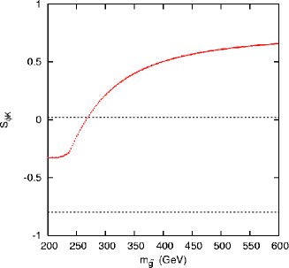
(a) $\Delta_{\rm hard}=\Delta_{\rm annih}=0$

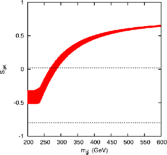
(b) $\rho_{\rm hard}\leq 1,\Delta_{\rm annih}=0$

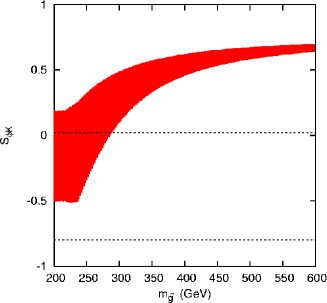
(c) $\Delta_{\rm hard}=0,\rho_{\rm annih}\leq 1$

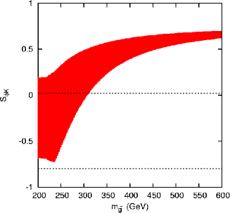
(d) $\rho_{\rm hard}\leq 1,\rho_{\rm annih}\leq 1$

Figure 9: Range of $S_{\phi K}$ predicted in the BBNS approach for several parametrizations of the subleading uncertainties, as a function of $m_{\tilde{g}}$. In (a), all subleading uncertainties are taken to be zero. In (b) and (c), hard scattering and annihilation corrections are each included. In (d), both are. Plots take $(\delta^{d}_{23})_{RR}$ to generate most negative $S_{\phi K}$, for $m_{\tilde{g}}=250$ GeV and $x=1$.

VII Higgs-mediated FCNCs

At large $\tan\beta$, FCNCs can also be mediated by exchange of neutral Higgs bosons, as found in $B\rightarrow X_{s}l^{+}l^{-}$ huang , $B_{s,d}\rightarrow\mu^{+}\mu^{-}$ kolda and $\tau\rightarrow 3\mu$ Babu:2002et , etc. In this paper we consider the same mechanism leading to $b\rightarrow ss\bar{s}$. Unlike the gluino mediated amplitudes, which generate flavor independent amplitudes for $b\rightarrow sq\bar{q}$, the Higgs exchange diagrams generate flavor-dependent amplitudes since the Higgs coupling is proportional to the Yukawa couplings. Therefore $b\rightarrow ss\bar{s}$ can be modified by a significant amount, whereas $b\rightarrow su\bar{u}$ or $b\rightarrow sd\bar{d}$ remain essentially unchanged. Thus decays such as $B\to\phi K_{S},\eta^{(}{}^{\prime}{}^{)}K$ can be affected by Higgs exchange, whereas $B\rightarrow\pi K$, $\pi\pi$ modes are not.

In the presence of Higgs-mediated FCNCs (Fig. 1(c)), new operators $O_{\{R,L\},S}$ and $O_{\{R,L\},P}$ appear in the $\Delta B=1$ effective Hamiltonian:

$$H_{\rm eff}\rightarrow H_{\rm eff}-\frac{G_{F}}{\sqrt{2}}V_{ts}^{*}V_{tb}~{}\left[C_{R,S}O_{R,S}+C_{R,P}O_{R,P}+(R\rightarrow L)\right]$$ (19)

where

$$O_{R,S}=(\overline{s}_{L}b_{R})~{}(\overline{s}s),~{}~{}~{}O_{R,P}=(\overline{s}_{L}b_{R})~{}(\overline{s}\gamma_{5}s)$$ (20)

where the first index $R$ or $L$ denotes the chirality of the initial $b$ quark in the $B$ meson, and color is conserved pairwise. In the MSSM with minimal flavor violation, the Wilson coefficients $C_{L,S}$ and $C_{L,P}$ are suppressed relative to $C_{R,S}$ and $C_{R,P}$ by $m_{s}/m_{b}$, and will be ignored in the following. The explicit form of $C_{R,S(P)}$ due to the neutral Higgs exchange is given by

$$C_{R,S}\simeq-C_{R,P}\simeq{\alpha\over\pi}\,\left({\tan^{3}\beta\over 4\sin^{2}\theta_{W}}\right)\,\left({m_{b}m_{\mu}m_{t}\mu\over M_{W}^{2}M_{A}^{2}}\right)\,{\sin 2\theta_{\tilde{t}}\over 2}\,f(m_{\tilde{t_{1}}}^{2},m_{\tilde{t_{2}}}^{2},\mu^{2}).$$ (21)

where the loop function $f(a,b,c)$ can be found in Refs. kolda , for example. Note that the $O_{R,S}-O_{R,P}$ operator is equivalent to $-O_{6}$ after Fierz transformation (but without summing over all flavors, only with $\bar{s}s$).

In a model with minimal flavor violation (as defined in Ref. mfv ) the phases of the SUSY contributions would match those of the SM and so no new source of CP violation would be generated. However, if we extend minimal flavor violation to allow arbitrary phases (a definition used by other authors), we can allow our $C_{R,S}$ and $C_{R,P}$ operators to be complex and contribute to $S_{\phi K}$. Therefore we will assume that the new operators have complex coefficients with $O(1)$ phases.

However the Wilson coefficients $C_{R,S}$ and $C_{R,P}$ also generate $B_{s}\rightarrow\mu^{+}\mu^{-}$, which has been and is being searched for actively at the Tevatron. The upper limit on this decay from CDF cdf during the Tevatron’s Run I is

$$B(B_{s}\rightarrow\mu^{+}\mu^{-})<2.6\times 10^{-6}.$$ (22)

The relevant effective Hamiltonian is

$$H_{\rm eff}(B_{s}\rightarrow\mu^{+}\mu^{-})=-{G_{F}\over\sqrt{2}}~{}V_{tb}V_{ts}^{*}\left[C_{R,S}(\bar{s}_{L}^{\alpha}b_{R}^{\alpha})~{}(\bar{\mu}\mu)+C_{R,P}(\bar{s}_{L}^{\alpha}b_{R}^{\alpha})~{}(\bar{\mu}\gamma_{5}\mu)+(R\rightarrow L)\right].$$ (23)

Note that the Wilson coefficients $C_{R,S(P)}$ here are essentially the same as those that appear in the effective Hamiltonian for $b\rightarrow ss\bar{s}$, up to a small difference between the muon and the strange quark masses (or their Yukawa couplings). We find that the current upper limit (22) puts rather a strong constraint on $C_{R,S(P)}$:

$$|C_{R,S}|,|C_{R,P}|\lesssim 0.005,$$

since

$$\mbox{B}(B_{s}\rightarrow\mu\mu)\propto\left|C_{R,S}\right|^{2}+\left|C_{R,P}\right|^{2}.$$ (24)

We then find that $S_{\phi K}$ cannot be smaller than 0.71 for such small values of $C_{R,S(P)}$ within the naive factorization approach. Thus it appears impossible to explain the large deviation in $S_{\phi K}$ with Higgs-mediated $b\rightarrow ss\bar{s}$ alone.

Recently the authors of Ref. cheng have re-examined this issue in models with non-minimal flavor violation. Among other things, they allow a large $(\bar{b}_{L}s_{R})(\bar{s}s)$ operator, though one would normally expect such an operator to be suppressed by $m_{s}/m_{b}$ with respect to the $(\bar{b}_{R}s_{L})(\bar{s}s)$ operator. The authors of Ref. cheng argue that one can explain the data on $S_{\phi K}$ without violating the CDF bound on $B_{s}\to\mu\mu$ if one allows the original operator and its parity conjugate to both be large and roughly the same size.

Since our explanation for $S_{\phi K}$ involves non-minimal flavor violation, we should in principle allow similar violation in the Higgs operators. In the general case the branching fraction for $B_{s}\to\mu\mu$ depends on

$$\mbox{B}(B_{s}\to\mu\mu)\propto\left|C_{R,S}-C_{L,S}\right|^{2}+\left|C_{R,P}-C_{L,P}\right|^{2}$$ (25)

rather than Eq. (24) above. It would then appear that our limit applies to this difference rather than the coefficients individually isidori . The authors of Ref. cheng make use of this to find a region of parameter space consistent with negative $S_{\phi K}$.

However, this is not the complete story. Because the couplings and masses in the MSSM Higgs sector are highly constrained (e.g., $m_{H}\simeq m_{A}$), the scalar and pseudoscalar coefficients are tied to one another. In particular, one finds that

$$C_{R,S} \simeq -C_{R,P}$$

$$C_{L,S} \simeq +C_{L,P}$$

where the approximate equality becomes exact for $m_{A}\gg m_{Z}$. Thus Eq. (25) can be rewritten as:

$$\mbox{B}(B_{s}\to\mu\mu)\propto\left|C_{R,S}-C_{L,S}\right|^{2}+\left|C_{R,S}+C_{L,S}\right|^{2}=2\left(\left|C_{R,S}\right|^{2}+\left|C_{L,S}\right|^{2}\right).$$ (26)

Our argument from the CDF bound applies as before, and we see no way to use Higgs mediation to generate $S_{\phi K}<0$, at least in this way.

VIII Motivating $(\delta_{LR,RL}^{d})_{23}$ of $O(10^{-2})$

In this section, we want to provide some motivation for $(\delta_{LR}^{d})_{23}\sim 10^{-2}$ that we find phenomenologically is needed to generate $S_{\phi K}$. Conversely, considerations such as those in this section show how one might use data to point toward classes of string–based theories. At this stage, we are not advocating any model of $(\delta_{LR}^{d})_{23}\sim 10^{-2}$, but rather showing that $(\delta_{LR}^{d})_{23}$ of the needed size can be theoretically plausible.

Before going to a specific construction, we write down the generic expression for the flavor parameters $(\delta)_{LR}$ in a supergravity Lagrangian (which is the low energy effective field theory derived from a string theory model). Under the assumption that either the Yukawa coupling does not depend on the moduli fields, or it is a function of moduli times some constant proportional to the Yukawa coupling itself, we can write the trilinear couplings as kobayashi

$$\tilde{A}^{f}_{ij}\propto(A_{L}\cdot Y^{f}+Y^{f}\cdot A_{R})_{ij},$$ (27)

where $A_{L}$ and $A_{R}$ are $3\times 3$ diagonal matrices, and $f=u,d$. We also neglect a term which is proportional to a constant times the Yukawa matrix which will not affect the prediction of $(\delta)_{ij}$. The mass insertions $\delta_{LR}^{f}$ are defined as the ratio between the off diagonal elements and the diagonal ones of the squark mass matrices in the superCKM basis. The superCKM basis is defined by rotating the quark superfields by $V_{L}^{f}$ and $V_{R}^{f}$, where $V_{L}^{f}Y^{f}V_{R}^{f\dagger}=Y_{\mathtt{diag}}$. Then we obtain the expression for the relevant LR mass insertions in the general MSSM as

$$(\delta_{LR})_{ij,i\neq j} \propto m^{f}_{j}(A_{2}^{L}-A_{1}^{L})(V_{L})_{i2}(V_{L}^{*})_{j2}+m^{f}_{j}(A_{3}^{L}-A_{1}^{L})(V_{L})_{i3}(V_{L}^{*})_{j3}$$

$$+ m^{f}_{i}(A_{2}^{R}-A_{1}^{R})(V_{R})_{i2}(V_{R}^{*})_{j2}+m^{f}_{i}(A_{3}^{R}-A_{1}^{R})(V_{R})_{i3}(V_{R}^{*})_{j3},$$

where $A_{i}^{L,R}$ are model dependent parameters of order the gravitino mass, $m_{3/2}$. The most important feature of this expression is that the sizes of various terms are proportional to SM fermion masses $m^{f}_{i,j}$. Some of the immediate conclusions one can draw from this observation are

• $(\delta_{LR})_{12}\ll(\delta_{LR})_{13},(\delta_{LR})_{23}$.

• $\delta^{u}/\delta^{d}\sim m^{u}/m^{d}$. In particular, $(\delta^{u}_{LR})_{23}/(\delta^{d}_{LR})_{23}\sim m_{t}/m_{b}$.

Note that these are relations obtained at some high energy scale. However, the dominant RGE runnings of the trilinears are diagonal in the superCKM basis. Therefore, those relation also hold approximately at low energy scale.

We now turn to a possible string theory motivated scenario where those features can arise. For definiteness, we focus on the models constructed from a intersecting D5-brane setup. Suppose we have two stacks of D5-branes intersecting at $90^{\circ}$. There are six compact dimensions which are grouped into three complex pairs labeled by $i=1,2,3$. D-branes are objects on which open strings can end. Open string sectors in this type of scenario are classified by (i) which D-brane it ends on, and (ii) which complex dimension it moves in. We will have the following open string states Ibanez:1998rf

• $C^{5_{i}}_{j}$: open strings which end on the $5_{i}$ brane and move along the $j$th complex compact dimension.

• $C^{5_{i}5_{j}}$: open strings which start from the $5_{i}$ brane and end on the $5_{j}$ brane.

The string theory selection rules permit two type of large couplings (provided they are gauge invariant): $C^{5_{i}}_{i}C^{5_{i}}_{j}C^{5_{i}}_{k}$ and $C^{5_{i}}_{j}C^{5_{i}5_{k}}C^{5_{i}5_{k}}$, where $i\neq j\neq k$.

The next question is how to embed the MSSM matter content into the this scenario. Since we need some large mixing between the last two generations, one obvious choice is to embed them identically, i.e., assign them to the same open string sector. However, this type of construction has a problem because it also predicts $A_{2}^{L}=A_{3}^{L}$ which is not desirable. Therefore, we have to embed the last two generations into different open string sectors and yet give them a large mixing.

Suppose we have the following embedding of the MSSM matter content into open string sectors, adopting the notation that $F_{i}$ and $\overline{F}_{i}$ are the $i$th generation left and right handed quarks, respectively.

• The Higgs field: $h=\frac{1}{\sqrt{2}}(C^{5_{1}}_{1}+C^{5_{1}}_{2})$.

• The quarks:

  $$F_{3}=C^{5_{1}}_{2}, \overline{F}_{3}=C^{5_{1}}_{3}$$

  $$F_{2}=C^{5_{1}}_{1}, \overline{F}_{2}=C^{5_{1}}_{3}$$

  $$F_{1}=C^{5_{1}5_{2}}, \overline{F}_{1}=C^{5_{1}5_{2}}.$$ (29)

From the string theory selection rules, we can then determine the Yukawa coupling matrix to be

$$Y\propto\left(\begin{array}[]{ccc}\cdot&\cdot&\cdot\\ \cdot&1&1\\ \cdot&1&1\end{array}\right).$$ (30)

We can also work out the soft supersymmetry breaking terms Brignole:1997dp . In particular, the trilinear couplings are

$$\frac{\tilde{A}}{-\sqrt{3}m_{3/2}} = -\frac{1}{\sqrt{2}}(X_{0}+X_{3})\cdot Y+\left(\begin{array}[]{ccc}\frac{1}{2}X_{0}+X_{1}+\frac{1}{2}X_{3}&&\\ &X_{1}+X_{3}&\\ &&X_{0}+X_{1}\end{array}\right)\cdot Y$$ (34)

$$+ Y\cdot\left(\begin{array}[]{ccc}-\frac{1}{2}X_{0}+X_{2}-\frac{1}{2}X_{3}&&\\ &1&\\ &&1\end{array}\right),$$ (38)

where $X_{i}$’s are complex parameters satisfying $\sum_{i=0}^{3}|X_{i}|^{2}=1$. Notice now we have written the trilinear couplings in the form of Eq. (27). We have singled out the part which is the Yukawa matrix multiplied by a diagonal matrix proportional to the identity since this term is diagonal in the super-CKM basis and does not contribute to flavor violating processes. We also have the following expressions for soft masses

$$m^{2}_{F_{3}} = m^{2}_{3/2}(1-3|X_{3}|^{2})$$

$$m^{2}_{F_{2}} = m^{2}_{3/2}(1-3|X_{0}|^{2})$$

$$m^{2}_{\bar{F}_{3}} = m^{2}_{3/2}(1-3|X_{2}|^{2})$$

$$m^{2}_{\bar{F}_{2}} = m^{2}_{3/2}(1-3|X_{2}|^{2}).$$ (39)

Using Eq. (VIII), our ansatz for the Yukawa textures and the definition of the mass insertion parameter, we then have the following estimate for the size of $(\delta^{d}_{LR})_{23}$:

$$(\delta^{d}_{LR})_{23}\sim\frac{\sqrt{3}m_{b}}{m_{3/2}}\frac{(X_{0}-X_{3})}{\sqrt{(1-3|X_{0}|^{2})(1-3|X_{2}|^{2})}}.$$ (40)

Clearly, this can be as large as of order $\sim 0.01$. It can also have a quite nontrivial phase structure since $X_{0}$ and $X_{3}$ are in general complex parameters.

Notice however in this particular implementation, we will generically have $(\delta^{d}_{RR})_{23}\sim 0$ since $m^{2}_{\bar{F}_{3}}=m^{2}_{\bar{F}_{2}}$. We can also choose $(\delta^{d}_{LL})_{23}$ to be close to zero by setting $|X_{0}|\approx|X_{3}|$.

As remarked above, this model suggests $(\delta_{LR}^{u})_{23}\sim{m_{t}\over m_{b}}~{}(\delta^{d}_{LR})_{23}$, so $(\delta^{d}_{LR})_{23}\sim 0.008$ suggests $(\delta_{LR}^{u})_{23}\sim 0.3$. Such a large value is not in conflict with any data on $B\rightarrow X_{s}\gamma$ or $B\rightarrow X_{s}l^{+}l^{-}$, which give essentially no constraint on $(\delta_{LR}^{u})_{23}$ Buras:1997ij . Also $(\delta_{LR}^{u})_{23}\sim 0.3$ can generate a flavor changing top decay $t\rightarrow cg$ only up to $(6.0,8.5,9.2)\times 10^{-6}$ for $x=(0.5,1,3)$ and $m_{\tilde{g}}=400$ GeV, which are still below the threshold for observability ($\sim 10^{-5}$) at future colliders such as LHC and NLC. Another prediction of this model is $(\delta_{LR}^{d})_{12}\sim 5\times 10^{-5}$, which could dominate $\epsilon^{{}^{\prime}}/\epsilon_{K}$ through the chromomagnetic $s\rightarrow dg$ transition.

Let us also comment on the size of $(\delta^{d}_{RL})_{23}$ in our current embedding. From our formula for the trilinears, we see that $(\delta^{d}_{RL})_{23}=(\delta^{d*}_{LR})_{32}$ is determined by $(A^{R}_{2,3}-A^{R}_{1})V_{R}V_{R}^{*}$. In our current embedding, we have $A^{R}_{2}=A^{R}_{3}$ since the last two generations of the right-handed (s)quarks have the same embedding. We can then use the unitarity of $V_{R}$ to simplify the expression of $(\delta^{d}_{RL})_{23}$ to $(\delta^{d}_{RL})_{23}\propto\frac{m_{b}}{m_{3/2}}(V_{R})_{31}(V_{R})^{*}_{21}$ which is suppressed by higher powers of $\lambda$. However, we can realize a larger $(\delta^{d}_{RL})_{23}$ by simply switching the open string embedding of the last two generations of left-handed and right-handed (s)quarks, $F_{2,3}$ and $\overline{F}_{2,3}$. Then we can have a sizable $(\delta^{d}_{RL})_{23}\sim 0.01$ while $(\delta^{d}_{LR})_{23}$ is suppressed by the higher power of $\lambda$.

Before closing this section, let us comment on the mass mixings/insertions that would be generated by the RG running from the high energy scale to electroweak scale. If we assume a universal boundary condition for scalar masses at the reduced Planck scale $M_{*}\simeq 2.4\times 10^{18}$ GeV, and all $(\delta_{AB})_{ij}$ are zero at the high energy scale, nonnegligible values are induced by renormalization group (RG) running. The approximate solutions to the RG equation for the left squark mass squared becomes

$$(m_{LL}^{2})_{ij}(\mu=M_{weak})\simeq-{1\over 8\pi^{2}}\,Y_{t}^{2}\left(V_{\rm CKM}\right)_{3i}\left(V_{\rm CKM}^{*}\right)_{3j}\,\left(3m_{0}^{2}+a_{0}^{2}\right)\,\log({M_{*}\over M_{\rm weak}}),$$

and one can estimate $(\delta_{LL}^{d})_{23}\simeq 9\times 10^{-3}$. Note that this parameter is real however, since $V_{23}$ and $V_{33}$ are real in the Wolfenstein parameterization. Also other mass insertions are further suppressed by additional factors of $Y_{d}$ and $Y_{d}^{2}$, so that $|(\delta_{LR,RL}^{d})_{23}|\sim 10^{-5}$ and $|(\delta_{RR}^{d})_{23}|\sim 10^{-7}$. These are too small to explain a large shift of $S_{\phi K}$ relative to $S_{\psi K}$.

In some SUSY GUT scenarios, the large mixing in the neutrino sector induces a large mixing in the right squark sector through the analogous RG running. The resulting mixing is about moroi

$$(\delta_{RR}^{d})_{23}\simeq 2\times 10^{-2}\,\left({M_{\nu_{R}}\over 10^{14}~{}{\rm GeV}}\right).$$

Therefore the $RR$ mixing is generically larger than $LL$ mixing in SUSY GUTs where the see-saw mechanism is generating the nonvanishing neutrino masses. Still it cannot affect $S_{\phi K}$ by a large amount as discussed in the previous section, although the size of $(\delta_{RR}^{d})_{23}$ could be $\sim O(0.5)$ with a new complex phase so that $B_{s}^{0}$–$\bar{B}_{s}^{0}$ mixing could be significantly shifted.

On the other hand, if the SUSY flavor problem is resolved by the alignment mechanism using some spontaneously broken flavor symmetries, or decoupling (the effective SUSY models), the resulting $LL$ or $RR$ mixings in the $23$ sector could be easily order of $\sim\lambda^{2}$ ($\lambda\equiv\sin\theta_{c}\approx 0.22$) with either $LL>>RR$, $LL<<RR$ or $LL\approx RR$ align ; decoupling , whereas the mixing in the 13 sector is further suppressed by additional power(s) of $\lambda$(’s) in order to avoid large contributions to $B^{0}$–$\bar{B}^{0}$ mixing. These parameters will carry CP violating phases in general and can contribute significantly to $\Delta M_{s}$ and $\sin 2\beta_{s}$.

Further, in the presence of an $LL$ or $RR$ insertion, there can be an induced $LR$ or $RL$ insertion when $\mu\tan\beta$ is large with respect to the scalar masses, due to the double mass insertions ko01 ; bjkp :

$$(\delta_{LR}^{d})_{23}^{\rm ind}=(\delta_{LL}^{d})_{23}\times{m_{b}(A_{b}-\mu\tan\beta)\over\tilde{m}^{2}}.$$

In case $(\delta_{LL,RR}^{d})_{23}\sim 10^{-2}$, one can achieve $(\delta_{LR,RL}^{d})_{23}^{\rm ind}\sim 10^{-2}$, if $\mu\tan\beta\sim 30\,$TeV. This could be natural if $\tan\beta$ is large $\sim 40$. For larger $LL,RR$ mixing, even smaller $\mu\tan\beta$ would suffice to induce the needed $LR,RL$ mass insertions of a size $10^{-2}-10^{-3}$. Since the $\delta_{LL,RR}$’s in SUSY flavor models are generically complex, the induced $(\delta_{LR}^{d})_{23}^{\rm ind}$ could carry a new CP violating phase bjkp , which can again explain a large negative $S_{\phi K}$. Also, the $RR$ insertion can have a phase inherited from the neutrino mixing matrix in a SUSY GUT model, which would be transferred to the induced $RL$ insertion moroi . Therefore the induced $RL$ insertion can explain the observed $S_{\phi K}$ in SUSY GUT models. On the other hand, the phase of $(\delta_{LL}^{d})_{23}$ for the case of minimal SUGRA is given by the CKM matrix elements, and it is real for the 2-3 mixing. Therefore the induced $(\delta_{LR}^{d})_{23}^{\rm ind}$ in SUGRA-like models is incapable of explaining the negative $S_{\phi K}$.

IX Conclusions

Recent data has given us hope that there may be new physics lurking in rare $B$-decays, particularly $B\to\phi K_{S}$. In this paper, we considered several potentially important SUSY contributions to this process in order to see if a significant deviation in its time-dependent CP asymmetry $S_{\phi K}$ could arise from SUSY effects. In particular, we considered the SUSY gluino contributions in models with non-minimal flavor violation, and the Higgs-mediated contributions in models with minimal flavor violation. While the latter has the advantage of only affected the $b\to ss\bar{s}$ transition, current bound on $B_{s}\to\mu^{+}\mu^{-}$ at Fermilab constrain the relevant operators to be too small. Models based on the $LL$ and $RR$ insertions in gluino interaction vertices also give contributions too small to alter $S_{\phi K}$ very much, unless gluinos are very light (close to the experimental bounds). However, in an $LL$ or $RR$ scenario one expects an impending observation of gluinos and squarks, and absence of $B_{s}^{0}$–$\bar{B}_{s}^{0}$ oscillations at the Tevatron, since $\Delta M_{s}$ increases dramatically in the $LL$ ($RR$) case when $S_{\phi K}<0$.

On the other hand, gluino-mediated $LR$ or $RL$ contributions can generate sizable effects in $S_{\phi K}$ as long as $|(\delta_{LR,RL}^{d})_{23}|\sim 10^{-3}$ – $10^{-2}$. As a by-product, we found that nonleptonic $B$ decays such as $B\to\phi K_{S}$ are beginning to constrain $|(\delta_{LR,RL}^{d})_{23}|$ as strongly as $B\rightarrow X_{s}\gamma$. We also studied various correlations among $S_{\phi K}$, $C_{\phi K}$, the direct CP asymmetry in $B\rightarrow X_{s}\gamma$, $\Delta M_{s}$, $A_{\ell\ell}$ and $\sin 2\beta_{s}$. Using the $LR$ or $RL$ insertions, it is easy to obtain a negative $S_{\phi K}$ without conflict with any other observables. Furthermore, there are definite correlations among $S_{\phi K}$, $C_{\phi K}$ and $A_{\rm CP}^{b\to s\gamma}$, and our explanation for the negative $S_{\phi K}$ can be easily tested by measuring these other correlated observables. In particular $C_{\phi K}$ can be positive only for the $RL$ insertion. For this case, the direct CP asymmetry in $B\rightarrow X_{s}\gamma$ vanishes (assuming no $RR$ insertion is present), unlike the case of the $LR$ or $LL$ insertions. In a scenario with both $RL$ and $RR$ insertions, the resulting direct CP asymmetry in $B\rightarrow X_{s}\gamma$ could be as large as in the $LR$ mixing case, and there could be a large, complex contributions to $B_{s}^{0}$–$\bar{B}_{s}^{0}$ mixing, leading to significant effects in $\Delta M_{s}$ and $\sin 2\beta_{s}$. The effects of the (pure) $LR$ and $RL$ insertions on $B_{s}^{0}$–$\bar{B}_{s}^{0}$ are rather small and it would be difficult to distinguish our model from the SM by the $B_{s}^{0}$–$\bar{B}_{s}^{0}$ mixing, considering various theoretical and experimental uncertainties.

Thus, we have found that three classes of supersymmetric models could not naturally explain a negative time dependent CP asymmetry $S_{\phi K}$ in $B\to\phi K_{S}$ if the initial hints of such an asymmetry should persist when data improves: $LL$, $RR$ insertions, and Higgs-dominated decays. Two other classes, $LR$ and $RL$ insertions, can explain the data and can be distinguished to some extent with more and better data. Insertions of the size and kind needed can be generated naturally in simple string-motivated models and SUSY flavor models.