Scattering of color dipoles: from low to high energies

Abstract

A dipole-dipole scattering amplitude is calculated exactly in the first two orders of perturbation theory. This amplitude is an analytic function of the relative energy and the dipoles’ sizes. The cross section of the dipole-dipole scattering approaches the high-energy BFKL asymptotics starting from a relatively large rapidity $\sim 5$.

I Introduction

It is well known that the effective degrees of freedom at high energies are so-called Wilson lines - infinite gauge factors ordered along the velocities of the colliding particles (for a review, see Ref. mobzor, ). Let us consider the classical example of the scattering of virtual photons in QCD. The photons decompose into quark-antiquark pairs which interact by exchanging gluons. At high energies, quarks move very fast so that their propagation in the background fields of the exchange gluons is reduced to the gauge factor of $U^{n}(x_{\perp})$ nacht

$$U^{n}(x_{\perp})=Pe^{ig\int_{-\infty}^{\infty}dun_{\mu}A^{\mu}(un+x_{\perp})}$$ (1)

ordered along the classical trajectory of the particle, i.e. a straight line collinear to the velocity $n$. Here $x_{\perp}$ is the transverse position (an impact parameter) of the fast quark, which does not change in the collision. The propagation of a quark-antiquark pair is described by the color dipole kop formed from the two Wilson lines

$$W^{n}(x_{\perp},y_{\perp})={\rm Tr}\{U^{n}(x_{\perp})U^{n\dagger}(y_{\perp})\}$$ (2)

where $x_{\perp}$ and $y_{\perp}$ are the transverse positions (impact parameters) of quark and antiquark. The high-energy $\gamma^{\ast}\gamma^{\ast}$ scattering reduces then to the dipole-dipole amplitude integrated over dipoles’ sizes and separations (see Fig. 1):

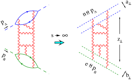
Figure 1: High-energy scattering as a dipole-dipole amplitude. Wavy lines are gluons and dashed lines are Wilson gauge factors (1)

.

$$A(s)~{}=~{}{s\over 2}\int d^{2}a_{\perp}d^{2}b_{\perp}~{}I^{A}(a_{\perp})I^{B}(b_{\perp})T(a_{\perp},b_{\perp};s)$$ (3)

where $I^{A}(a_{\perp})$ is the so-called “impact factor” (see Appendix A) and $T(a_{\perp},b_{\perp};s)$ is the dipole-dipole scattering amplitude:

$$T(a_{\perp},b_{\perp};s)~{}=$$ (4)

$$-i\!\int\!d^{2}z_{\perp}\langle W^{n}(a_{\perp}+z_{\perp},z_{\perp})~{}W^{e}(b_{\perp},0_{\perp})\rangle~{}.$$

Here $e$ is the unit vector in the direction of the motion of the second virtual photon. The collision energy is related to the relative rapidity $\eta$ ($\equiv$ angle between the dipoles)

$${p_{A}\cdot p_{B}\over\sqrt{p_{A}^{2}p_{B}^{2}}}=n\cdot e=\cosh\eta~{}.$$ (5)

The energy dependence of the $\gamma^{\ast}\gamma^{\ast}$ amplitude is governed by the evolution of the dipoles with respect to the slope of Wilson lines determined by $\eta$ npb96 ; prdpl .

We see that the dipole-dipole amplitude is an “elementary” high-energy scattering process. Moreover, in theories without asymptotic particle states (like N=4 SYM) the dipole-dipole scattering is the only way to access the high-energy behavior of amplitudes. Also, there have been many attempts to estimate the high-energy behavior of hadron-hadron amplitudes using non-perturbative models for the dipole-dipole scattering (see Ref. dosch, for a review). For hadrons, the impact factors cannot be calculated in pQCD; however, they can be related to the hadron wave functions.

The usual phenomenological approach to dipole-dipole scattering in pQCD is to take the light-like dipoles. However, matrix elements of the light-like Wilson operators contain longitudinal divergencies. In the LLA we cut these divergencies “by hand”mu94 ; nn . This prescription - take the light-like

dipoles and cut the divergencies by hand - seems to avoid ambiguities in the next-to-leading order, toobalbel . However, to go beyond perturbation theory one has to consider the scattering of the off-light-cone dipoles. The dipole-dipole amplitude is then a function of the dipole separations and the angle $\theta$ ($\sim$ relative rapidity $\eta$) between the dipoles. If this amplitude is an analytic function of $\theta$, one can calculate the dipole-dipole scattering (a correlation function of two infinite rectangular Wilson loops) in the Euclidean region and continue to the Minkowski space. In the recent series of papers zahed ; pesch the dipole-dipole scattering was calculated in the Euclidean space using the AdS-CFT correspondence and continued analytically as a function of the angle $\theta$ to the Minkowski space, where $\theta\rightarrow i\eta$. Another example of such analytic continuation is the calculation of the instanton-induced dipole-dipole ampltitude dodik .

To be able to obtain the high-energy behavior from the Euclidean amplitudes it is crucial to verify that the dipole-dipole amplitude is an analytic function of $\theta$. In Ref. meggio, this statement was proved for the correlation function of two Wilson rectangles with a finite longitudinal length ${\cal T}$ (see also Ref. pirner, ). At finite${\cal T}$, the amplitude is an analytic function of the angle $\theta$ between the rectangles. In the limit ${\cal T}\rightarrow\infty$, one recovers the dipole-dipole scattering amplitude. However, whether the ${\cal T}\rightarrow\infty$ limit commutes with the analytic continutation from the Euclidean to Minkowski space is an open question. We demonstrate with an explicit calculation in the first two orders of perturbation theory that the dipole-dipole amplitude is, indeed an analytic function of the angle between the dipoles (as well as of the dipoles’ sizes). This is the first important result of our paper. We see that the analyticity survives the ${\cal T}\rightarrow\infty$ limit in the first two orders of perturbation theory, and presumably it happens in all higher orders as well so that the dipole-dipole amplitude appears to be an analytic function of $\theta$.

The second result of our paper concerns the rate at which the dipole-dipole amplitude approaches the BFKL asymptotics. At sufficiently high energies, the cross section for the “unpolarized” dipole-dipole scattering is given by the BFKL formula

$$\sigma(a,b;\eta)\sim{\alpha_{s}^{2}\over ab}\int d\nu\Big{(}{a\over b}\Big{)}^{2i\nu}\eta^{{\alpha_{s}\over\pi}N_{c}\chi(\nu)}$$ (6)

where $\chi(\nu)=-\Re\psi(1/2+i\nu)-C$ is the position of the “hard pomeron”bfkl (for a review, see Ref. lobzor, ). The asymptotics of the $\gamma^{\ast}\gamma^{\ast}$ scattering is then given by Eq. (3). The formula (6) is obtained in the so-called leading log approximation (LLA), when $\alpha_{s}\ll 1,\alpha_{s}\ln s\sim\alpha_{s}\eta\sim 1$. The main problem with the LLA result (6) is that its power behavior $s^{4{\alpha_{s}\over\pi}N_{c}\ln 2}$ violates the Froissart bound $\ln^{2}s$ at asymptotically large $s$. Thus, the BFKL pomeron gives only the pre-asymptotic behavior at “moderately high” energies. It is a common belief that the true asymptotics at $s\rightarrow\infty$ (where $\alpha\ln s\gg 1$) comes from the unitarization of the BFKL pomeron. Despite numerous efforts, the high-energy asymptotics satisfying the Froissart bound is still an unsolved problem in QCD (for a recent discussion see Refs. mcler02, ; wkov02, ; kozlevin, ). In this paper, we address a different problem (important for mid-energy accelerators) - when does the LLA asymptotics start making sense - at 1, 10 , or 100 GeV? To get a complete answer to this question one should calculate the amplitude exactly and compare it to the BFKL asymptotics (6). Since it seems to be an impossible task at present, we calculate the dipole-dipole scattering in the first two orders of perturbation theory exactly and compare it to the asymptotic form. Our main result is that the asymptotics starts rather late, at $\eta\sim 5$, which translates into $\sqrt{s}\sim$=10 GeV for the scattering of dipoles with the $\rho$-meson size $a\sim 0.3fm$.

The paper is organized as follows. In Sect. 2 we calculate the dipole-dipole amplitude and the cross section in the leading order of perturbation theory. In the second order, we have calculated independently both the dipole-dipole amplitude and its imaginary part proportional to the cross section. Since the structure of the diagrams and the result is much more transparent for the cross section, in Sect. 3 we present only the results for the amplitude in the second order and leave the details until Sect. 5, where we give the detailed calculation of the dipole-dipole cross section. We discuss the effects due to the running coupling constant in Sect 4. Sect 6 contains the numerical estimates of the dipole-dipole cross section and Sect. 7 is devoted to the discussion of our results and an outlook. The explicit form of the second-order amplitudes is given in the Appendix.

II Dipole-dipole scattering in the Born approximation

We consider the dipole-dipole scattering amplitude defined as follows

$$T(x_{1\perp},x_{2\perp};x_{3\perp},x_{4\perp};\eta)$$ (7)

$$=~{}-i\langle W^{n}(x_{1\perp},x_{2\perp})W^{e}(x_{3\perp},_{4\perp})\rangle~{}.$$

Strictly speaking, the Wilson lines forming the dipole are connected with gauge links at infinity, so

$$T(x_{1\perp},x_{2\perp};x_{3\perp},x_{4\perp};\eta)$$

$$=~{}-i\lim_{{\cal T}\rightarrow\infty}\langle W^{n}_{\cal T}(x_{1\perp},x_{2\perp})W^{e}_{\cal T}(x_{3\perp},x_{4\perp})\rangle$$ (8)

where $W^{n}_{\cal T}$ is a rectangular Wilson loop of longitudinal length ${\cal T}$

$$W^{n}_{\cal T}(x_{1\perp},x_{2\perp})={\rm Tr}\{U_{\cal T}^{n}(x_{1\perp})[x_{1\perp}-{{\cal T}\over 2}n,x_{2\perp}-{{\cal T}\over 2}n]$$

$$\times~{}U_{\cal T}^{n\dagger}(x_{2\perp})[x_{1\perp}+{{\cal T}\over 2}n,x_{2\perp}+{{\cal T}\over 2}n]\}$$ (9)

and $U_{\cal T}^{n}(x_{1\perp})\equiv[{{\cal T}\over 2}n+x_{1\perp},-{{\cal T}\over 2}n+x_{1\perp}]$ etc. Hereafter, we use the notation

$$[x,y]\equiv Pe^{ig\int_{0}^{1}du(x-y)^{\mu}A_{\mu}(ux+(1-u)y)}sec:$$ (10)

for the straight-line ordered gauge link suspended between the points $x$ and $y$.

Since the gluons reduce to the pure gauge fields at infinity, the precise form of a contour connecting the points $x_{1\perp}\pm{{\cal T}\over 2}n$ and $x_{2\perp}\pm{{\cal T}\over 2}n$ does not matter. Moreover, we use Feynman gauge for the gluon propagator, and in this gauge the links at infinity do not contribute to the amplitude. Thus, we omit them in what follows to simplify the notations.

II.1 Cross section of the dipole-dipole scattering and optical theorem for dipoles

The total cross section of the scattering of the dipole of size $a$ on the dipole of size $b$ may be defined as

$$\sigma(a_{\perp},b_{\perp};\eta)~{}=~{}\int\!dz_{\perp}\varsigma(a_{\perp}+z_{\perp};z_{\perp},b_{\perp};\eta)$$ (11)

where

$$\varsigma(x_{i\perp},\eta) \equiv \sum_{X\neq 0}\langle 0|W_{ij}^{n\dagger}(x_{1\perp},x_{2\perp})W_{kl}^{e\dagger}(x_{3\perp},x_{4\perp})|X\rangle$$ (12)

$$\times \langle X|W_{ji}^{n}(x_{1\perp},x_{2\perp})W_{lk}^{e}(x_{3\perp},x_{4\perp})|0\rangle$$

is the total amplitude of the dipole-dipole transition into hadrons. Here the summation goes over all the intermediate states except for the vacuum and

$$W^{n}_{ij}(x_{1\perp},x_{2\perp})$$ (13)

$$=~{}\lim_{{\cal T}\rightarrow\infty}\Big{(}U_{\cal T}^{n}(x_{1\perp})[x_{1\perp}-{{\cal T}\over 2}n,x_{2\perp}-{{\cal T}\over 2}n]U_{\cal T}^{n\dagger}(x_{2\perp})\Big{)}_{ij}~{}.$$

If we include the intermediate vacuum state in the r.h.s. of Eq. (12), we get $N_{c}^{2}$ due to the completeness relation. Separating the non-interacting contribution in a usual way

$$\langle 0|W^{n}(x_{1\perp},x_{2\perp})W^{e}(x_{3\perp},x_{4\perp})|0\rangle=N_{c}^{2}+iT(x_{i},\eta)\,$$ (14)

we get the “optical theorem” for the dipole-dipole scattering:

$$\Im T(x_{1\perp},x_{2\perp};x_{3\perp},x_{4\perp};\eta)=~{}{1\over 2}\varsigma(x_{1\perp},x_{2\perp};x_{3\perp},x_{4\perp};\eta)~{}.$$ (15)

It is worth noting that the high-energy $\gamma^{\ast}\gamma^{\ast}$ cross section reduces to the dipole cross section (12) integrated with impact factors, similar to the Eq. (3) for the amplitude:

$$A(s)~{}=~{}{1\over 4}\int d^{2}a_{\perp}d^{2}b_{\perp}~{}I^{A}(a_{\perp})I^{B}(b_{\perp})\sigma(a_{\perp},b_{\perp};\eta)$$ (16)

We will calculate the dipole-dipole cross section in two ways: directly as the r.h.s. of Eq. (12) or via the optical theorem as the imaginary part of eq. (7).

II.2 Lowest order dipole-dipole amplitude

In the leading order of perturbation theory, the correlation function of two Wilson-line operators is proportional to the (massless) two-dimensional propagator:

$$\langle U^{n}(x_{\perp})U^{e}(y_{\perp})~{}=~{}-\langle U^{n}(x_{\perp})U^{e\dagger}(y_{\perp})\rangle$$

$$=~{}ig^{2}\coth\eta\int\!{{\textstyle d}\lower 0.12915pt\hbox{\kern-3.80005pt${}^{\scriptstyle-}$}\kern-0.50003pt{}^{2}k_{\perp}\over k_{\perp}^{2}}~{}e^{i(k,x-y)_{\perp}}$$ (17)

where $(a,b)_{\perp}$ denotes the (positive) scalar product of two-dimensional vectors $\vec{a}_{\perp}$ and $\vec{b}_{\perp}$. (For brevity, we use the $\hbar$-inspired notations ${\textstyle d}\lower 0.12915pt\hbox{\kern-3.80005pt${}^{\scriptstyle-}$}\kern-0.50003pt{}^{n}k\equiv{d^{n}k\over(2\pi)^{n}}$ and ${\textstyle\delta}\lower 0.12915pt\hbox{\kern-3.80005pt${}^{\scriptstyle-}$}\kern-0.50003pt{}^{(n)}(k)\equiv(2\pi)^{n}\delta^{(n)}(k)$).

The relevant Feynman diagrams are shown in Fig. 2.

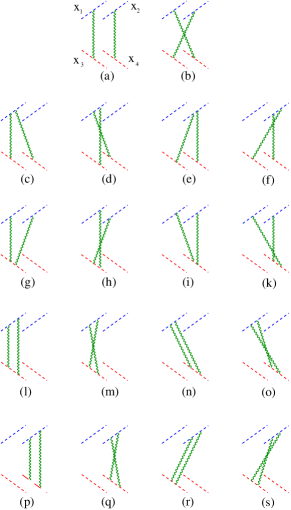
Figure 2: Dipole-dipole scattering in the lowest order of perturbation theory

The contribution of these diargams has the form:

$$T(x_{1\perp},x_{2\perp};x_{3\perp},x_{4\perp};\eta)$$ (18)

$$=~{}ig^{4}\coth^{2}\eta~{}{N_{c}^{2}-1\over 8}\int\!{d^{2}k_{1\perp}d^{2}k_{2\perp}\over 16\pi^{4}k_{1\perp}^{2}k_{2\perp}^{2}}$$

$$\times~{}(e^{-i(k_{1},x_{1})_{\perp}}-e^{-i(k_{1},x_{2})_{\perp}})(e^{i(k_{1},x_{3})_{\perp}}-e^{i(k_{1},x_{4})_{\perp}})$$

$$\times~{}(e^{i(k_{2},x_{1})_{\perp}}-e^{i(k_{2},x_{2})_{\perp}})(e^{-i(k_{2},x_{3})_{\perp}}-e^{-i(k_{2},x_{4})_{\perp}})$$

The integral over the transverse momenta can be performed explicitly, resulting in

$$T(x_{1\perp},x_{2\perp};x_{3\perp},x_{4\perp};\eta)$$

$$=~{}i{N_{c}^{2}-1\over 8}\alpha_{s}^{2}\left(\ln{x^{2}_{13}x^{2}_{24}\over x^{2}_{23}x^{2}_{14}}\right)^{2}\coth^{2}\eta$$ (19)

where $x_{12}\equiv x_{1\perp}-x_{2\perp}$ etc. (cf. Ref. kozlevin, )

II.3 Dipole-dipole cross section in the Born approximation

As we mentioned above, the dipole-dipole cross section can be obtained in two ways: via the optical theorem as the imaginary part of Eq. (19) or, directly, as the r.h.s. of Eq. (14). Since the amplitude in the lowest order in $\alpha_{s}$ is purely imaginary, the “unintegrated cross section” (12) is

$$\varsigma(x_{i\perp};\eta)~{}=~{}g^{4}{N_{c}^{2}-1\over 4}\coth^{2}\eta~{}\left(\ln{x^{2}_{13}x^{2}_{24}\over x^{2}_{23}x^{2}_{14}}\right)^{2}~{}.$$ (20)

For future use, it is instructive to calculate $\varsigma(x_{i\perp},\eta)$ directly as the r.h.s. of Eq. (12). In this case, Feynman rules for the calculation of the cross sections can be reproduced by a functional integral over the double set of fields (see e.g. keld ): (+) to the right of the cut and (-) to the left with the propagators

$$A^{a\mu}_{\pm}(x)A^{b\nu}_{\pm}(y) = \!\int\!{dk\over 16\pi^{4}}e^{-ik(x-y)}{ig^{\mu\nu}\delta^{ab}\over\mp k^{2}-i\epsilon}$$ (21)

$$A^{a\mu}_{-}(x)A^{b\nu}_{+}(y) = -\!\int\!{dk\over 16\pi^{4}}e^{-ik(x-y)}g^{\mu\nu}\delta^{ab}2\pi\delta(k^{2})\theta(k_{0})$$

These correspond to the Cutkovsky rules for the cross sections.

In these notations, the dipole-dipole cross section reads (cf. difope )

$$\varsigma(x_{i\perp};\eta) = \langle{\rm Tr}\{W^{n}_{(-)}(x_{1\perp},x_{2\perp})W^{n}_{(+)}(x_{1\perp},x_{2\perp})\}$$ (22)

$$\times ~{}{\rm Tr}\{W^{e}_{(-)}(x_{3\perp},x_{4\perp})W^{e}_{(+)}(x_{3\perp},x_{4\perp})\}\rangle$$

The relevant diagram is shown in Fig. (3).

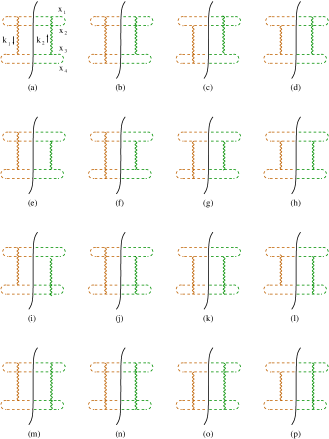
Figure 3: Cross section of the dipole-dipole scattering in the lowest order of perturbation theory

To emphasize that here we have only the gauge links at ${\cal T}=-\infty$ we draw them explicitly.

The leading-order correlation function of Wilson lines in $(+)$ sector is given by Eq. (17) and in $(-)$ sector by Eq. (17) with a different sign

$$\langle U_{(+)}^{n}(x_{\perp})U_{(+)}^{e}(y_{\perp})~{}=~{}-\langle U_{(+)}^{n}(x_{\perp})U_{(+)}^{e\dagger}(y_{\perp})\rangle$$

$$=~{}-\langle U_{(-)}^{n}(x_{\perp})U_{(-)}^{e}(y_{\perp})~{}=~{}\langle U_{(-)}^{n}(x_{\perp})U_{(-)}^{e\dagger}(y_{\perp})\rangle$$

$$=~{}ig^{2}\coth\eta\int\!{d^{2}k_{\perp}\over 4\pi^{2}k_{\perp}^{2}}~{}e^{i(k,x-y)_{\perp}}$$ (23)

Using Eq. (23) it is easy to see that

$${4\over N_{c}^{2}-1}\varsigma(x_{1\perp},x_{2\perp};x_{3\perp},x_{4\perp};\eta)$$

$$=~{}g^{4}\coth^{2}\eta\int\!{d^{2}k_{1\perp}d^{2}k_{2\perp}\over 16\pi^{4}k_{1\perp}^{2}k_{2\perp}^{2}}(e^{-i(k_{1},x_{1})_{\perp}}-e^{-i(k_{1},x_{2})_{\perp}})$$

$$\times~{}(e^{i(k_{1},x_{3})_{\perp}}-e^{i(k_{1},x_{4})_{\perp}})~{}(e^{i(k_{2},x_{1})_{\perp}}-e^{i(k_{2},x_{2})_{\perp}})$$

$$\times~{}(e^{-i(k_{2},x_{3})_{\perp}}-e^{-i(k_{2},x_{4})_{\perp}})$$ (24)

where the $2^{4}=16$ terms correspond to 16 diagrams in Fig. 3). Integrating over $k_{\perp}$, we reproduce the optical-theorem result (20).

III Second-order amplitude

In the next order of perturbation theory there are too many diagrams to present them all - rougly speaking, we must take the diagrams in Fig. 2 and add an extra gluon line in all possible ways. Let us consider the diagram in Fig. 2a. If we insert the gluon line in all possible ways to connect the left and the right parts of the diagram in Fig. 2a, we get the diagrams shown in Fig. 4.

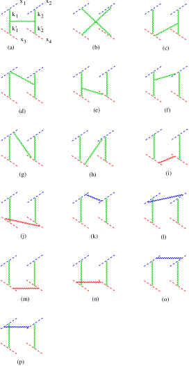
Figure 4: Typical “connected ” diagrams for the dipole-dipole amplitude.

Also, we can insert a gluon line in the left or right part only and get the “disconnected” diagrams shown in Fig. 5.

Not all the diagrams for the correlator of two Wilson loops (7) contribute to the dipole-dipole scattering amplitude. There are two exceptional classes of diagrams proportional to the total time of the evolution ${\cal T}$. First, there are those shown in Fig. 5 q-t, which describe “mass renormalization” of Wilson lines. Their contribution has the usual form of $\delta mL$, where $\delta m$ is the self-energy correction and $L\simeq 2{\cal T}$ is the perimeter of the Wilson loop corresponding to the dipole. Similarly, the diagrams in Fig. 4 m-p contribute to the “binding energy” $\epsilon$ of the dipole and lead to $\epsilon{\cal T}$ terms. These two contributions exponentiate so that one obtains:

$$-i\langle{\rm Tr}\{U_{\cal T}^{n}(x_{1})U_{\cal T}^{n\dagger}(x_{2})\}~{}{\rm Tr}\{U_{\cal T}^{n}(x_{3})U_{\cal T}^{n\dagger}(x_{4})\}\rangle$$ (25)

$$=~{}e^{-4i\delta m{\cal T}-i(\epsilon_{12}+\epsilon_{34}){\cal T}}~{}T(x_{1\perp},x_{2\perp},x_{3\perp},x_{4\perp},\eta;{\cal T})$$

where $T(x_{i\perp},\eta;{\cal T})$ describes the dipole-dipole scattering at the time ${\cal T}$. The resulting amplitude

$$T(x_{i\perp},\eta)=\lim_{{\cal T}\rightarrow\infty}T(x_{i\perp},\eta;{\cal T})$$ (26)

$$=~{}\lim_{{\cal T}\rightarrow\infty}-i\langle{\rm Tr}\{U_{\cal T}^{n}(x_{1})U_{\cal T}^{n\dagger}(x_{2})\}~{}{\rm Tr}\{U_{\cal T}^{n}(x_{3})U_{\cal T}^{n\dagger}(x_{4})\}$$

$$\hskip 142.26378pt\times~{}e^{4i\delta m{\cal T}+i(\epsilon_{12}+\epsilon_{34}){\cal T}}$$

is finite as ${\cal T}\rightarrow\infty$. In the second order of perturbation theory, the multiplication in r.h.s. of eq. (26) reduces to the subtraction of the corresponding terms ($4\delta m{\cal T}$ and $2\epsilon{\cal T}$). The result is that the diagrams in Fig. 4 m-p and Fig. 5 q-t are left out and in the diagrams in Fig. 4 i-l and Fig. 5 m-p the color factor $-{1\over 2N_{c}}$ is replaced by $-{1\over 2N_{c}}-c_{F}=-{N_{c}\over 2}$.

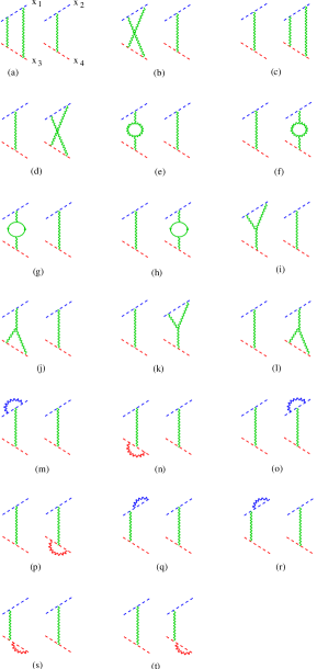
Figure 5: ‘’Disconnected” diagrams for the dipole-dipole amplitude.

Thus, we are left with the diagrams shown in Fig. 4a-j and 5a-r. Also, there are $\sim 20$ times more diagrams which are obtained from the addition of an extra gluon to the graphs in Fig. 2b,c,…s. The calculation of these diagrams is standard but lengthy. In Sect. V we will present some details of the (independent) calculation of the imaginary part of this amplitude where the structure of diagrams is much more transparent. Here we will only give the final result for the amplitude and discuss which classes of diagrams contribute to it.

We have performed calculation of the dipole-dipole amplitude in both the Euclidean and Minkowski spaces. In the Euclidean space, this amplitude is a correlation function of two Wilson rectangles at angle $\theta$ such as $\cos\theta=n\cdot e$. In both cases, the $g^{6}$ amplitude has the form (in Euclidean space $\eta=i\theta$):

$$T(x_{i\perp},\eta)~{}=~{}{ig^{6}\over 4\pi}{N_{c}(N_{c}^{2}-1)\over 8}\coth^{2}\eta$$ (27)

$$\times\int\!{\textstyle d}\lower 0.12915pt\hbox{\kern-3.80005pt${}^{\scriptstyle-}$}\kern-0.50003pt{}^{2}k_{1}{\textstyle d}\lower 0.12915pt\hbox{\kern-3.80005pt${}^{\scriptstyle-}$}\kern-0.50003pt{}^{2}k_{2}{\textstyle d}\lower 0.12915pt\hbox{\kern-3.80005pt${}^{\scriptstyle-}$}\kern-0.50003pt{}^{2}k^{\prime}_{1}{\textstyle d}\lower 0.12915pt\hbox{\kern-3.80005pt${}^{\scriptstyle-}$}\kern-0.50003pt{}^{2}k^{\prime}_{2}~{}(e^{-i(k_{1},x_{1})}-e^{-i(k_{1},x_{2})})$$

$$\times~{}(e^{-i(k^{\prime}_{1},x_{3})}-e^{-i(k^{\prime}_{1},x_{4})})(e^{i(k_{2},x_{1})}-e^{i(k_{2},x_{2})})$$

$$\times~{}(e^{i(k^{\prime}_{2},x_{3})_{\perp}}-e^{i(k^{\prime}_{2},x_{4})_{\perp}})~{}\Bigg{\{}{\textstyle\delta}\lower 0.12915pt\hbox{\kern-3.80005pt${}^{\scriptstyle-}$}\kern-0.50003pt{}^{2}(k_{1}+k^{\prime}_{1}-k_{2}-k^{\prime}_{2})$$

$$\times~{}\Bigg{[}{A(k_{i};\eta)\over(k_{1}+k^{\prime}_{1})^{6}}+i\pi{(N_{c}^{2}-4)\coth\eta\over N^{2}_{c}(k_{1}+k^{\prime}_{1})_{\perp}^{2}}\Big{(}{1\over k_{1}^{2}{k^{\prime}}^{2}_{2}}+{1\over k_{2}^{2}{k^{\prime}}^{2}_{1}}\Big{)}\Bigg{]}$$

$$+~{}{\textstyle\delta}\lower 0.12915pt\hbox{\kern-3.80005pt${}^{\scriptstyle-}$}\kern-0.50003pt{}^{2}(k_{1}+k^{\prime}_{1}){\textstyle\delta}\lower 0.12915pt\hbox{\kern-3.80005pt${}^{\scriptstyle-}$}\kern-0.50003pt{}^{2}(k_{2}+k^{\prime}_{2})~{}\Bigg{[}-\Big{(}\eta-{i\pi\over 2}+{i\pi\over 2}{N_{c}^{2}-4\over N_{c}^{2}}\Big{)}$$

$$\times~{}\coth\eta\int\!{\textstyle d}\lower 0.12915pt\hbox{\kern-3.80005pt${}^{\scriptstyle-}$}\kern-0.50003pt{}^{2}p~{}\Big{\{}{k_{1}^{2}\over p^{2}(k_{1}-p)^{2}}+{k_{2}^{2}\over p^{2}(k_{2}-p)^{2}}\Big{\}}$$

$$+~{}{1\over 2\pi}\ln{\mu^{2}\over|k_{1}||k_{2}|}\Big{(}{5\over 3}-{n_{f}\over 2N_{c}}\Big{)}+{1\over\pi}\ln\mu^{2}|x_{12}||x_{34}|\Bigg{]}\Bigg{\}}~{}.$$

Here $\mu$ is the normalization point of the $\overline{MS}$ scheme. The explicit form of the function $A(k_{1},k^{\prime}_{1},k_{2},k^{\prime}_{2};\eta)$ is given in the Appendix B. Note that they are analytical functions of $\eta$ and $k_{i\perp}^{2}$ with singularities at $\eta\rightarrow 0$ corresponding to the bound state of two parallel dipoles.

The r.h.s. of Eq. (27) consists of two terms. The first term comes from the diagrams of the type shown in Fig. 4. (The $N_{c}^{2}-4$ term is the odderon contribution coming from the structure $d^{abc}d^{abc}$). The first expression of the second term comes from the “gluon reggeization” diagrams in Fig. 5 a-d, while the second one ($\sim{5\over 3}-{2n_{f}\over 3N_{c}}$) comes from the gluon and quark self-energy shown in Fig. 5 e-h. The diagrams in Fig.5 i-l vanish (cf. Ref. hquarks, ), while the terms coming from Fig.5 m-p are the pure divergency $\sim\int{d^{2}k_{\perp}\over k_{\perp}^{2}}$ which also vanishes in the framework of dimensional regularization(see the discussion in next Section). It is easy to see that the apparent divergency at $k+k^{\prime}\rightarrow 0$ in the gluon reggeizatoon terms cancels with the corresponding contribution to $A(k_{i};\eta)$ (see Eq. 54).

The main conclusion from the Eq. (27) is that the dipole-dipole amplitude is an analytic function of the angle $\eta$. It is easy to check that the functions $A$ become real as $\eta\rightarrow i\theta$ (see the Appendix B) and so does the amplitude $iT(x_{i\perp},i\theta)$.

It is worth noting that in the LLA (as $\eta\rightarrow\infty$) we reproduce the first iteration of the BFKL kernel

$$T(x_{i\perp},\eta)~{}\stackrel{{\scriptstyle\eta\rightarrow\infty}}{{\rightarrow}}~{}{ig^{6}\eta\over 4\pi}{N_{c}(N_{c}^{2}-1)\over 4}$$ (28)

$$\times\int\!{\textstyle d}\lower 0.12915pt\hbox{\kern-3.80005pt${}^{\scriptstyle-}$}\kern-0.50003pt{}^{2}k_{1}{\textstyle d}\lower 0.12915pt\hbox{\kern-3.80005pt${}^{\scriptstyle-}$}\kern-0.50003pt{}^{2}k_{2}{\textstyle d}\lower 0.12915pt\hbox{\kern-3.80005pt${}^{\scriptstyle-}$}\kern-0.50003pt{}^{2}k^{\prime}_{1}{\textstyle d}\lower 0.12915pt\hbox{\kern-3.80005pt${}^{\scriptstyle-}$}\kern-0.50003pt{}^{2}k^{\prime}_{2}~{}(e^{-i(k_{1},x_{1})}-e^{-i(k_{1},x_{2})})$$

$$\times~{}(e^{-i(k^{\prime}_{1},x_{3})}-e^{-i(k^{\prime}_{1},x_{4})})(e^{i(k_{2},x_{1})}-e^{i(k_{2},x_{2})})$$

$$\times~{}(e^{i(k^{\prime}_{2},x_{3})_{\perp}}-e^{i(k^{\prime}_{2},x_{4})_{\perp}})~{}{\textstyle\delta}\lower 0.12915pt\hbox{\kern-3.80005pt${}^{\scriptstyle-}$}\kern-0.50003pt{}^{2}(k_{1}+k^{\prime}_{1}-k_{2}-k^{\prime}_{2})$$

$$\times~{}\Bigg{[}-{(k_{1}-k_{2})^{2}\over k_{1}^{2}k_{2}^{2}{k^{\prime}_{1}}^{2}{k^{\prime}_{2}}^{2}}+{k_{1}^{-2}{k^{\prime}_{2}}^{-2}+k_{2}^{-2}{k^{\prime}_{1}}^{-2}\over{k^{\prime}_{2}}^{2}(k_{1}+k^{\prime}_{1})^{2}}$$

$$-~{}{\textstyle\delta}\lower 0.12915pt\hbox{\kern-3.80005pt${}^{\scriptstyle-}$}\kern-0.50003pt{}^{2}(k_{1}+k^{\prime}_{1})\int\!{\textstyle d}\lower 0.12915pt\hbox{\kern-3.80005pt${}^{\scriptstyle-}$}\kern-0.50003pt{}^{2}p~{}\Big{\{}{k_{1}^{2}\over p^{2}(k_{1}-p)^{2}}+{k_{2}^{2}\over p^{2}(k_{2}-p)^{2}}\Big{\}}\Bigg{]}~{}.$$

IV Running coupling constant

As we shall see below, the diagrams contributing to the renormalization of coupling constant are somewhat unusual: as in the case of a heavy-quark potential ${\alpha_{s}(r)\over r}$, the coefficient ${11\over 3}N_{c}-{2n_{f}\over 3}$ in front of $\ln\mu$ comes from both the UV- and the IR-divergent diagrams (cf. hquarks ).To see how it happens, it is instructive to start with the scattering of the light-like dipoles where the diagrams for the renormalization of coupling constant are the usual UV-divergent vertices and self-energies shown in Fig. 6.

As we mentioned above, the scattering amplitude for the light-like dipoles is not a well-defined quantity because of the longitudinal divergencies corresponding to $\eta=\infty$ coming from the diagrams in Fig. 4 a-h and Fig. 5 a-d. If we cut this divergency “by hand”, we get the asymptotical contribution, i.e. Eq. (28). Apart from this contribution, the only non-zero diagrams are those shown in Fig. 5 e-h. They lead to the renormalization of coupling constant in Eq. (19).

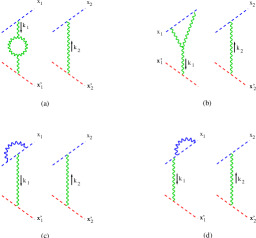
Figure 6: Running coupling constant for the light-like dipoles

Standard computation of these diagrams yields

$$\Big{[}\Big{(}{5\over 3}N_{c}-{2n_{f}\over 3}\Big{)}+2N_{c}\Big{]}~{}{g^{2}\over 16\pi^{2}}\ln{\mu^{2}\over k_{1\perp}^{2}}$$ (29)

where $\Big{(}{5\over 3}N_{c}-{2n_{f}\over 3}\Big{)}$ comes from the diagram in Fig. 6a and the similar diagram with the quark loop (see Fig. 5o), while $2N_{c}$ comes from the diagram in Fig. 6b. It turns out that the diagram in Fig. 6c vanishes, while the diagram in Fig. 6d is irrelevant since it contributes only to the “mass renormalization” $\delta m$ of the Wilson line (see Eq. (25)).

Surprisingly, the structure of the diagrams contributing to the running coupling constant is quite different for even slightly off-the-light-cone dipoles. In this case the diagram in Fig. 6a is the same as for the light-like dipoles, the diagram in Fig. 6b vanishes, and the diagram in Fig. 6c is a pure divergency of the type $\int{dp_{\perp}\over p_{\perp}^{2}}$, which must be set to zero in the dimensional regularization approach. Following Ref. hquarks it is convenient to write down this term as

$${g^{2}N_{c}\over 8\pi^{2}}\Big{(}{2\over 4-d}-{2\over d-4}\Big{)}$$ (30)

The UV pole ${2\over 4-d}$ together with the pole coming from the diagram in Fig. 6a forms ${2\over 4-d}{g^{2}\over 16\pi^{2}}\Big{(}{11\over 3}N_{c}-{2\over 3}n_{f}\Big{)}$, while the IR pole ${2\over d-4}$ cancels with similar poles in the diagrams in Fig. 7.

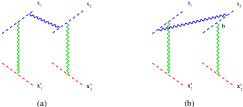
Figure 7: IR divergent diagrams contributing to the renormalization of the coupling constant

Due to “cancellation” between the UV and IR contributions to Fig. 6c, in order to reproduce the running-coupling coefficient $\Big{(}{11\over 3}N_{c}-{2\over 3}n_{f}\Big{)}$ in front of $\ln\mu^{2}$ in the dimensional regularization, one should take into account not only the “usual” UV divergent diagrams in Fig. 6 but also the IR-divergent diagrams in Fig. 7 (cf. diplom ). As a result the coefficient $\Big{(}{5\over 3}N_{c}-{2n_{f}\over 3}\Big{)}$ in front of ${g^{2}\over 16\pi^{2}}\ln\mu^{2}$ comes from the diagram in Fig. 6a, while ${g^{2}N_{c}\over 8\pi^{2}}\ln\mu^{2}$ comes from the diagrams in Fig. 7 (and all other diagrams in Fig. 6 vanish).

This mixture of the IR and UV divergencies could have been a source of a potential problem. The cornerstone of the BFKL approach is the assumption that all the $\ln s$ come from the longitudinal integrations, while the integrations over the transverse momenta are convergent at $k_{\perp}^{2}\sim m^{2}$, where $m$ is of order of masses (or virtualities) of the colliding particles. (After the summation of the BFKL ladder we have “diffusion” in the transverse momenta leading to $\ln k_{\perp}^{2}\sim\sqrt{\ln{s\over m^{2}}}$, but such terms do not spoil the “power counting” in $(\ln s)^{n}$). This assumption is not true for the diagrams leading to the renormalization of the coupling constant since they are UV divergent. However, the structure of these diagrams is very simple - they are 1-loop vertex and self-energy corrections, and after the subtraction of the ${1\over 4-d}$ poles the integrals over $k_{\perp}^{2}$ are bound with $\mu^{2}$. In our case, the structure of the integrals over the transverse momenta is more complicated due to the mixture of the IR and UV divergencies. There are individual diagrams where the upper cutoff in the integrals over the $k_{\perp}$ is the energy $\sqrt{s}$ rather than ${1\over a}$ or the normalization scale $\mu$. Such contributions would give the additional non-BFKL $\ln s$ terms coming from the logarithmical integrals over the transverse momenta $\int{dk_{\perp}\over k_{\perp}^{2}}$. Fortunately, we will see below that such terms cancel in the sum of all diagrams and the remaining transverse integrals are cut by the dipoles’ sizes (or by the normalization point $\mu$).

V Cross section

V.1 Calculation of Feynman diagrams

In the case of the cross section (12), the structure of the diagrams is more transparent and we will present some details of this calculation. In this order, there are two types of Feynman diagrams: one with gluon emission and one without. Typical diagrams of the first type are shown in Fig. 8.

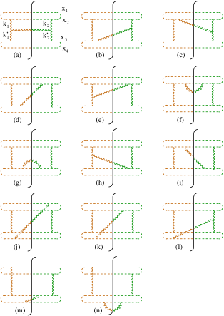
Figure 8: Typical diagrams for the dipole-dipole cross section with the emission of a real gluon

The sum of these diagrams is proportional to the square of the finite-energy Lipatov vertex $L^{\mu}(k_{1},k^{\prime}_{1})L_{\mu}(k_{2},k^{\prime}_{2})$. The Lipatov vertex

$$L(k_{1},k^{\prime}_{1}) = (k_{1}-k^{\prime}_{1})(ne)+\Big{[}2(k^{\prime}_{1}n)+{(ne)\over(k_{1}e)}{k^{\prime}}_{1}^{2}\Big{]}e$$ (31)

$$- \Big{[}2(k_{1}e)+{(ne)\over(k^{\prime}_{1}n)}k_{1}^{2}\Big{]}n$$

is a sum of the emissions of the real gluon with momentum $(k_{1}+k_{1}^{\prime})$ from the left part of the diagrams in Fig. 7 in all possible ways. This vertex is gauge-invariant:

$$(k_{1}+k^{\prime}_{1})^{\mu}L(k_{1},k^{\prime}_{1})=0$$ (32)

At infinite energies $(ne)\rightarrow\infty$ the expression (31) reduces to the usual asymptotic form of Lipatov vertex (see e.g. lobzor ).

The sum of the diagrams in Fig. 8 has the form

$${4\over N_{c}^{2}-1}\varsigma(x_{1\perp},x_{2\perp};x_{3\perp},x_{4\perp};\eta)_{\rm Fig.\ref{fig:dip7}}$$ (33)

$$=~{}g^{6}N_{c}\int\!{d^{4}k_{1}d^{4}k^{\prime}_{1}d^{4}k_{2}d^{4}k^{\prime}_{2}\over 128\pi^{7}k_{1}^{2}{k^{\prime}}_{1}^{2}k_{2}^{2}{k^{\prime}}_{2}^{2}}\delta^{(4)}(k_{1}+k^{\prime}_{1}-k_{2}-k^{\prime}_{2})$$

$$\times~{}\delta(k_{1}+k^{\prime}_{1})^{2}\theta(k_{1}+k^{\prime}_{1})_{0}~{}\delta(k_{1}\cdot n)\delta(k_{2}\cdot n)$$

$$\times~{}\delta(k^{\prime}_{1}\cdot e)\delta(k^{\prime}_{2}\cdot e)(e^{-i(k_{1},x_{1})_{\perp}}-e^{-i(k_{1},x_{2})_{\perp}})~{}$$

$$\times~{}(e^{i(k_{1},x_{3})_{\perp}}-e^{i(k_{1},x_{4})_{\perp}})~{}(e^{i(k_{2},x_{1})_{\perp}}-e^{i(k_{2},x_{2})_{\perp}})$$

$$\times~{}(e^{-i(k_{2},x_{3})_{\perp}}-e^{-i(k_{2},x_{4})_{\perp}})\Big{[}-L(k_{1},k^{\prime}_{1})\cdot L(k_{2},k^{\prime}_{2})\Big{]}~{}.$$

The explicit form of the product of two Lipatov vertices is

$$-L(k_{1},k^{\prime}_{1})\cdot L(k_{2},k^{\prime}_{2})~{}$$ (34)

$$=~{}{(ne)^{3}\over k_{1e}k^{\prime}_{1n}}(k_{1}^{2}{k^{\prime}}_{2}^{2}+k_{2}^{2}{k^{\prime}}_{1}^{2})+2(k_{1}-k_{2})^{2}(ne)^{2}$$

$$-~{}4({k^{\prime}}_{1n}^{2}+k_{1e}^{2})-2(ne)\Big{[}{k^{\prime}_{1n}\over k_{1e}}({k^{\prime}}_{1}^{2}+{k^{\prime}}_{2}^{2})+{k_{1e}\over k^{\prime}_{1n}}(k_{1}^{2}+k_{2}^{2})\Big{]}$$

$$-~{}(ne)^{2}\Big{[}{{k^{\prime}}_{1}^{2}{k^{\prime}}_{2}^{2}\over k_{1e}^{2}}+{k_{1}^{2}k_{2}^{2}\over{k^{\prime}}_{1n}^{2}}\Big{]}$$

where $k_{1e}\equiv(k_{1}\cdot e)$ and $k^{\prime}_{1n}\equiv(k^{\prime}_{1}\cdot n)$. Apart from the diagrams with the emission of a real photon, there are diagrams with an extra virtual photon. If, for example, we take the diagram in Fig. 3h and insert an extra gluon line in the left $(-)$ sector in all possible ways, we get the diagrams shown in Fig. 9. We do not display the diagrams corresponding to $\delta m$ or $\delta\epsilon$, see the discussion in Sect. II. The contribution of these diagrams vanishes here anyway since the phase factors $e^{-i(2m+\epsilon){\cal T}}$ and $e^{i(2m+\epsilon){\cal T}}$ coming from the left and from the right of the cut cancel out in the cross section. Again, this leads to the replacement of the color factors $-{1\over 2N_{c}}$ by $-{1\over 2N_{c}}-c_{F}=-{N_{c}\over 2}$ in the diagrams of the Fig.8m and Fig.9f-i type.

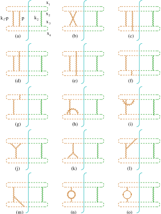
Figure 9: Typical diagrams with an extra virtual gluon

The calculation yields:

$${4\over N_{c}^{2}-1}\varsigma(x_{1\perp},x_{2\perp};x_{3\perp},x_{4\perp};\eta)_{\rm Fig.\ref{fig:dip8}}$$ (35)

$$=~{}{g^{4}N_{c}\coth^{2}\eta\over 4\pi}\int\!{d^{2}k_{1\perp}d^{2}k_{2\perp}\over 16\pi^{4}k_{1\perp}^{2}k_{2\perp}^{2}}$$

$$\times~{}(e^{-i(k_{1},x_{1})_{\perp}}-e^{-i(k_{1},x_{2})_{\perp}})(e^{i(k_{1},x_{3})_{\perp}}-e^{i(k_{1},x_{4})_{\perp}})$$

$$\times~{}(e^{i(k_{2},x_{1})_{\perp}}-e^{i(k_{2},x_{2})_{\perp}})(e^{-i(k_{2},x_{3})_{\perp}}-e^{-i(k_{2},x_{4})_{\perp}})$$

$$\times~{}\Bigg{[}-\eta\coth\eta\!\int\!{d^{2}p_{\perp}\over 4\pi^{2}p_{\perp}^{2}}\Big{(}{k_{1\perp}^{2}\over(k_{1}-p){\perp}^{2}}+{k_{1\perp}^{2}\over(k_{1}-p){\perp}^{2}}\Big{)}$$

$$+~{}{1\over 4\pi}\Big{(}\ln{\mu^{2}\over k_{1\perp}^{2}}+\ln{\mu^{2}\over k_{2\perp}^{2}}\Big{)}\Big{(}{5\over 3}-{2n_{f}\over 3N_{c}}\Big{)}\Bigg{]}$$

where the first “gluon reggeization” term comes from the diagrams in Fig. 9 a,b and the second from Fig. 9 n,o. As in the case of the amplitude, the diagrams in Fig. 9 j-m vanish and the diagrams in Fig. 9 h,i give rise to a pure divergency $\sim\int{dk_{\perp}\over k_{\perp}^{2}}$ that does not contribute in the framework of the dimensional regularization. (Instead, it leads to the “mixing” of the IR and UV singularities, see the discussion in Sect. IV). Finally, the diagrams in Fig. 9c-e cancel with the corresponding diagrams with an extra gluon to the right of the cut.

It is worth noting that the diagrams in Fig. 9 f,g should be regularized by finite ${\cal T}$ before calculation. After summation of all the relevant diagrams (e.g. Fig. 9 f,h and Fig. 8 g,m,n), the limit ${\cal T}\rightarrow\infty$ becomes regular.

Performing the remaining integrations over longitudinal momenta in Eq. 33 and the integration over $p$ in Eq. 35, one obtains

$$\varsigma(x_{1\perp},x_{2\perp};x_{3\perp},x_{4\perp},\eta)$$

$$=~{}{g^{6}N_{c}(N_{c}^{2}-1)\over 16\pi\tanh^{2}\eta}\int\!{\textstyle d}\lower 0.12915pt\hbox{\kern-3.80005pt${}^{\scriptstyle-}$}\kern-0.50003pt{}^{2}k_{1}{\textstyle d}\lower 0.12915pt\hbox{\kern-3.80005pt${}^{\scriptstyle-}$}\kern-0.50003pt{}^{2}k_{2}{\textstyle d}\lower 0.12915pt\hbox{\kern-3.80005pt${}^{\scriptstyle-}$}\kern-0.50003pt{}^{2}k^{\prime}_{1}{\textstyle d}\lower 0.12915pt\hbox{\kern-3.80005pt${}^{\scriptstyle-}$}\kern-0.50003pt{}^{2}k^{\prime}_{2}~{}$$ (36)

$$\times~{}(e^{-i(k_{1},x_{1})}-e^{-i(k_{1},x_{2})})(e^{-i(k^{\prime}_{1},x_{3})}-e^{-i(k^{\prime}_{1},x_{4})})$$

$$\times~{}(e^{i(k_{2},x_{1})}-e^{i(k_{2},x_{2})})(e^{i(k^{\prime}_{2},x_{3})_{\perp}}-e^{i(k^{\prime}_{2},x_{4})_{\perp}})$$

$$\times~{}~{}{\textstyle\delta}\lower 0.12915pt\hbox{\kern-3.80005pt${}^{\scriptstyle-}$}\kern-0.50003pt{}^{2}(k_{1}+k^{\prime}_{1}-k_{2}-k^{\prime}_{2})~{}{a(k_{i};\eta)\over(k_{1}+k^{\prime}_{1})^{6}}$$

$$+~{}{g^{2}N_{c}(N_{c}^{2}-1)\over 16\pi\tanh^{3}\eta}\!\int\!{{\textstyle d}\lower 0.12915pt\hbox{\kern-3.80005pt${}^{\scriptstyle-}$}\kern-0.50003pt{}^{2}k_{1\perp}{\textstyle d}\lower 0.12915pt\hbox{\kern-3.80005pt${}^{\scriptstyle-}$}\kern-0.50003pt{}^{2}k_{2}\over k_{1}^{2}k_{2}^{2}}$$

$$\times~{}(e^{-i(k_{1},x_{1})}-e^{-i(k_{1},x_{2})})(e^{i(k_{1},x_{3})}-e^{i(k_{1},x_{4})})$$

$$\times~{}(e^{i(k_{2},x_{1})}-e^{i(k_{2},x_{2})})(e^{-i(k_{2},x_{3})}-e^{-i(k_{2},x_{4})})$$

$$\times~{}\Bigg{[}-\eta\int\!{\textstyle d}\lower 0.12915pt\hbox{\kern-3.80005pt${}^{\scriptstyle-}$}\kern-0.50003pt{}^{2}p~{}\Big{\{}{k_{1}^{2}\over p^{2}(k_{1}-p)^{2}}+{k_{2}^{2}\over p^{2}(k_{2}-p)^{2}}\Big{\}}+$$

$$+~{}{1\over 2\pi}\ln{\mu^{2}\over|k_{1}||k_{2}|}\Big{(}{5\over 3}-{n_{f}\over 2N_{c}}\Big{)}+{1\over\pi}\ln\mu^{2}|x_{12}||x_{34}|\Bigg{]}~{}.$$

Here

$$a(k_{i};\eta)=\sum_{j=1}^{5}a_{j}(k_{i};\eta)$$ (37)

where $a_{1},a_{2},a_{3}$, $a_{4}$ and $a_{5}$ correspond to the first, second, third, fourth and fifth terms in Eq. (34), respectively. It should be mentioned that the fifth term in the r.h.s. of Eq. (34) is IR divergent. After regularization, in addition to $a_{5}(k_{i};\eta)$ it produces the $\ln\mu^{2}x_{12}x_{34}$ term which forms ${11\over 3}N_{c}-{2\over 3}n_{f}$ together with the contribution from the self-energy diagrams in Fig. 9 n,o.

The explicit form of the functions involved is:

$$a_{i}(k_{1},k_{2},k^{\prime}_{1},k^{\prime}_{2};\eta)~{}=~{}\Re A_{i}(k_{1},k_{2},k^{\prime}_{1},k^{\prime}_{2};\eta),$$ (38)

where $A_{i}$ can be found in the Appendix B. We see that the “unintegrated cross section” (36) is given by the imaginary part of the amplitude (27) (see the optical theorem for dipoles (15)).

The cross section of dipole-dipole scattering is given by the integral (11)

$$\sigma(\vec{a},\vec{b};\eta)~{}=~{}\int\!d^{2}z~{}\varsigma(\vec{a}+\vec{z},\vec{z},\vec{b},\vec{0};\eta)$$ (39)

V.2 Asymptotics of the cross section

As $\eta\rightarrow\infty$, the cross section (39) reduces to

$$\sigma_{\rm asy}(\vec{a},\vec{b};s)=$$ (40)

$$=~{}g^{4}(N_{c}^{2}-1)\int\!{{\textstyle d}\lower 0.12915pt\hbox{\kern-3.80005pt${}^{\scriptstyle-}$}\kern-0.50003pt{}^{2}k\over k^{2}}{{\textstyle d}\lower 0.12915pt\hbox{\kern-3.80005pt${}^{\scriptstyle-}$}\kern-0.50003pt{}^{2}k^{\prime}\over{k^{\prime}}^{2}}~{}4\sin^{2}{(k,a)\over 2}~{}\sin^{2}{(k^{\prime},b)\over 2}$$

$$\times~{}\Bigg{[}\Bigg{(}1+{g^{2}N_{c}\over 2\pi}~{}\Bigg{\{}-\eta\!\int\!{\textstyle d}\lower 0.12915pt\hbox{\kern-3.80005pt${}^{\scriptstyle-}$}\kern-0.50003pt{}^{2}p{k^{2}\over p^{2}(k-p)^{2}}$$

$$+~{}{1\over 4\pi}\ln{\mu^{2}\over k^{2}}\Big{(}{5\over 3}-{2n_{f}\over 3N_{c}}\Big{)}+{1\over 2\pi}\ln\mu^{2}ab\Bigg{\}}{\textstyle\delta}\lower 0.12915pt\hbox{\kern-3.80005pt${}^{\scriptstyle-}$}\kern-0.50003pt{}(k+k^{\prime})$$

$$+~{}{g^{2}N_{c}\over 2\pi}\Bigg{\{}{2\eta\over(k+k^{\prime})^{2}}+{\ln(k+k^{\prime})^{2}/k^{2}\over(k+k^{\prime})^{2}-k^{2}}\Big{(}{2k^{2}\over{k^{\prime}}^{2}}-1\Big{)}$$

$$+~{}{\ln(k+k^{\prime})^{2}/{k^{\prime}}^{2}\over(k+k^{\prime})^{2}-{k^{\prime}}^{2}}\Big{(}{2{k^{\prime}}^{2}\over k^{2}}-1\Big{)}-2{k^{2}+{k^{\prime}}^{2}\over k^{2}{k^{\prime}}^{2}}\Bigg{\}}\Bigg{]}+O(e^{-\eta})$$

It is easy to see that the integrals over the transverse momenta converge at $k_{\perp}^{2}\sim a^{-2}$. In the individual diagrams, the integrals over $k_{\perp}^{2}$ diverge (which means that they would be cut by $s$ in the corresponding exact expressions (39) and (36)), but in the sum of all diagrams such terms cancel (see the discussion in Sect. IV). The structure of the asymptotic result Eq. (40) is $\eta\sigma(a,b)$+$\sigma^{\prime}(a,b)$. The term $\sim\eta$ is the first iteration of the BFKL kernel. After integration over $k$ and $k^{\prime}$, it gives the first term in the expansion of $\eta^{\alpha_{s}\chi(\nu)}$ in powers of $\alpha_{s}$. The second term may be called the “dipole impact factor”. Indeed, the standard representation of the BFKL asymptotics of the cross section has the form

$$\sigma_{\rm asy}=\int\!{{\textstyle d}\lower 0.12915pt\hbox{\kern-3.80005pt${}^{\scriptstyle-}$}\kern-0.50003pt{}^{2}k\over k^{2}}{{\textstyle d}\lower 0.12915pt\hbox{\kern-3.80005pt${}^{\scriptstyle-}$}\kern-0.50003pt{}^{2}k^{\prime}\over{k^{\prime}}^{2}}I(a,k_{\perp})\eta^{K_{\rm BFKL}}I(b,k^{\prime}_{\perp})$$ (41)

where $K_{\rm BFKL}$ is the BFKL kernel (the LLA kernel + NLO BFKL kernel $+...$). The kernel terms come from the central region of the rapidity, while the impact factors come from the fringes of the longitudinal integral where the momentum of emitted gluon is almost collinear to $n$ or $e$. In this paper, we do not access the NLO BFKL terms nlobfkl (those would correspond to contributions to the amplitude $\sim\alpha_{s}^{4}\ln s$) so that all the non-LLA terms in Eq. (40) should be included in “impact factors” of the dipoles, namely,

$$I(b,k_{\perp})=\sin^{2}{(k,b)\over 2}+2\alpha_{s}k^{2}$$ (42)

$$\times~{}\int\!{{\textstyle d}\lower 0.12915pt\hbox{\kern-3.80005pt${}^{\scriptstyle-}$}\kern-0.50003pt{}^{2}k^{\prime}\over{k^{\prime}}^{2}}\Bigg{[}{\ln(k+k^{\prime})^{2}/k^{2}\over(k+k^{\prime})^{2}-k^{2}}\Big{(}{2k^{2}\over{k^{\prime}}^{2}}-1\Big{)}-{2\over{k^{\prime}}^{2}}\Bigg{]}\sin^{2}{(k^{\prime},b)\over 2}$$

and similarly for $I(a,k^{\prime}_{\perp})$. The impact factor(42) comes from the region of the longitudinal momenta in the emitted gluon close to $n$. Note that the integral in the r.h.s of Eq. (42) is convergent and behaves like $\ln k^{2}b^{2}$ for $k\rightarrow\infty$. Numerically, the $\alpha_{s}$ correction to the impact factor (42) is quite significant - it is responsible for the difference between the dotted and dash-dot lines in Fig. 10 below. (The NLO corrections to the virtual photon impact factor calculated recently also appear to be big, see Refs. bartelsimp, ; fadinimp, ).

V.3 Unpolarized dipole-dipole scattering

The “unpolarized” dipole-dipole scattering corresponds to the cross section (39) averaged over the orientation of the dipoles :

$$\sigma(a,b;s)~{}=~{}\int\!{d\theta_{a}\over 2\pi}{d\theta_{b}\over 2\pi}\sigma(\vec{a},\vec{b};s)$$ (43)

Note that in unpolarized $\gamma^{\ast}\gamma^{\ast}$ scattering the impact factor (52) depends only on $|\vec{a}|$ and $|\vec{b}|$ so the cross section of the unpolarized $\gamma^{\ast}\gamma^{\ast}$ scattering (3) is given by the “unpolarized” dipole-dipole cross section in Eq. (43) integrated over the dipole sizes with weights being impact factors

$$\sigma(a,b;\eta)~{}=~{}g^{4}(N_{c}^{2}-1)\coth^{2}\eta~{}$$ (44)

$$\times~{}\Bigg{\{}{g^{2}N_{c}\over 2\pi}\int\!{\textstyle d}\lower 0.12915pt\hbox{\kern-3.80005pt${}^{\scriptstyle-}$}\kern-0.50003pt{}^{2}k{\textstyle d}\lower 0.12915pt\hbox{\kern-3.80005pt${}^{\scriptstyle-}$}\kern-0.50003pt{}^{2}k^{\prime}~{}[1-J_{0}(ka)][1-J_{0}(k^{\prime}b)]~{}$$

$$\times~{}{a_{f}(k,k^{\prime};\eta)\over(k+k^{\prime})^{6}}~{}+~{}\int\!{{\textstyle d}\lower 0.12915pt\hbox{\kern-3.80005pt${}^{\scriptstyle-}$}\kern-0.50003pt{}^{2}k\over k^{4}}[1-J_{0}(ka)][1-J_{0}(kb)]$$

$$\times~{}\Bigg{(}1+{g^{2}N_{c}\over 2\pi}\Bigg{[}-\eta\coth\eta\!\int\!{\textstyle d}\lower 0.12915pt\hbox{\kern-3.80005pt${}^{\scriptstyle-}$}\kern-0.50003pt{}^{2}p~{}{k^{2}\over p^{2}(k-p)^{2}}$$

$$+~{}{1\over 4\pi}\Big{(}{5\over 3}-{2n_{f}\over 3N_{c}}\Big{)}\ln{\mu^{2}\over k^{2}}+{1\over 2\pi}\ln\mu^{2}ab\Bigg{]}\Bigg{)}\Bigg{\}}~{}.$$

The explicit form of the function $a_{f}(k,k^{\prime};\eta)$ is presented in the Appendix B.

VI Numerical estimates of the dipole-dipole cross section

For numerical estimates, let us consider the unpolarized scattering of equal-size dipoles. In this case we have only one-scale problem, so it is natural to take $\mu=a^{-1}$ where $a$ is the dipole size. The amplitude (44) reduces to

$$\sigma(a,a;\eta)~{}=~{}16\pi a^{2}\alpha^{2}_{s}(a)~{}\coth^{2}\eta~{}\Big{[}1+6\alpha_{s}(a)\Phi(\eta)\Big{]}$$ (45)

where

$$\Phi(\eta)$$ (46)

$$=~{}8\pi\!\int\!{\textstyle d}\lower 0.12915pt\hbox{\kern-3.80005pt${}^{\scriptstyle-}$}\kern-0.50003pt{}^{2}k{\textstyle d}\lower 0.12915pt\hbox{\kern-3.80005pt${}^{\scriptstyle-}$}\kern-0.50003pt{}^{2}k^{\prime}~{}[1-J_{0}(k)][1-J_{0}(k^{\prime})]~{}{a_{f}(k,k^{\prime};\eta)\over(k+k^{\prime})^{6}}$$

$$-~{}8\pi\!\int\!{{\textstyle d}\lower 0.12915pt\hbox{\kern-3.80005pt${}^{\scriptstyle-}$}\kern-0.50003pt{}^{2}k\over k^{2}}[1-J_{0}(k)]^{2}~{}\Bigg{[}\eta\coth\eta\!\int\!{{\textstyle d}\lower 0.12915pt\hbox{\kern-3.80005pt${}^{\scriptstyle-}$}\kern-0.50003pt{}^{2}p\over p^{2}(k-p)^{2}}+{\ln k\over 2\pi k^{2}}\Bigg{]}$$

where we have rescaled $k$ and $k^{\prime}$ by $a$ and took $n_{f}=N_{c}=3$. This expression should be compared to the asymptotical form (40) which gives

$$\sigma_{\rm asy}(a,a;\eta)~{}=~{}16\pi\alpha_{s}^{2}(a)a^{2}~{}\Big{[}1+6\alpha_{s}(a)\Phi_{\rm LLA+IF}(\eta)\Big{]}$$ (47)

where

$$\Phi_{\rm LLA+IF}=~{}8\pi\!\int\!{{\textstyle d}\lower 0.12915pt\hbox{\kern-3.80005pt${}^{\scriptstyle-}$}\kern-0.50003pt{}^{2}k\over k^{2}}{{\textstyle d}\lower 0.12915pt\hbox{\kern-3.80005pt${}^{\scriptstyle-}$}\kern-0.50003pt{}^{2}k^{\prime}\over{k^{\prime}}^{2}}~{}[1-J_{0}(k)]$$ (48)

$$\times~{}[1-J_{0}(k^{\prime})]~{}\Bigg{\{}{2\eta\over(k+k^{\prime})^{2}}+{\ln(k+k^{\prime})^{2}/k^{2}\over(k+k^{\prime})^{2}-k^{2}}\Big{(}{2k^{2}\over{k^{\prime}}^{2}}-1\Big{)}$$

$$+~{}{\ln(k+k^{\prime})^{2}/{k^{\prime}}^{2}\over(k+k^{\prime})^{2}-{k^{\prime}}^{2}}\Big{(}{2{k^{\prime}}^{2}\over k^{2}}-1\Big{)}-2{k^{2}+{k^{\prime}}^{2}\over k^{2}{k^{\prime}}^{2}}\Bigg{\}}$$

$$-~{}8\pi\!\int\!{{\textstyle d}\lower 0.12915pt\hbox{\kern-3.80005pt${}^{\scriptstyle-}$}\kern-0.50003pt{}^{2}k\over k^{4}}~{}[1-J_{0}(k)]^{2}~{}\Bigg{\{}\eta\!\int\!{\textstyle d}\lower 0.12915pt\hbox{\kern-3.80005pt${}^{\scriptstyle-}$}\kern-0.50003pt{}^{2}p~{}{k^{2}\over p^{2}(k-p)^{2}}+{\ln k\over 2\pi}\Bigg{\}}$$

is a sum of the LLA term $\sim\eta$ and the impact factor term $\sim$const. Numerically, $\Phi_{\rm LLA+IF}(\eta)\simeq 1.65(\eta-3.25)$ so

$$\sigma_{\rm asy}(a,a;\eta)~{}=~{}16\pi a^{2}\alpha^{2}_{s}(a)~{}\Big{[}1+9.88\alpha_{s}(a)(\eta-3.25)\Big{]}$$ (49)

where $\eta$ corresponds to the LLA approximation and -3.251 comes from the “dipole impact factor” (42). We have not calculated the next $\sim{1\over s}$ term in the asymptotic expansion (49) but the fit to the Figure 10 suggests the coefficient of order of 100 in front of it.

On Figure 10, we have depicted the comparison between the function $\Phi(\eta)$ describing the exact second-order cross section, its asymptotics $\Phi_{\rm LLA+IF}(\eta)$ Eq. (48) and the “pure” BFKL asymptotics $\Phi_{\rm LLA}(\eta)=1.64\eta$.

We have used the VEGAS algorithm of the Monte-Carlo technique with 10% accuracy to calculate the function $\Phi(\eta)$.

Figure 10: Exact cross section and its BFKL asymptotics. The solid line is Eq. (46), the dotted one is $\Phi_{\rm LLA+IF}$ Eq. (48) and the dashed line is $\Phi_{\rm LLA}=1.65\eta$

We see that the BFKL asymptotics starts rather late, at $\eta\sim 5$, which translates into $\sqrt{s}\sim~{}10$ GeV for the scattering of dipoles with the $\rho$-meson size $a\sim 0.25fm$. This is perhaps not surprising since even within the (collinearly improved cia ) NLO BFKL approximation itself the asymptotics starts relatively late, at $\eta\sim 6\div 8$ for the realistic dipoles trian . It should be emphasized, however, that these are two different theoretical questions relevant to the BFKL description of experimental cross sections: (i) how good is the BFKL approximation to the true high-energy asymptotics and (ii) when this true asymptotics starts making sense. For the second-order dipole-dipole scattering the first question is when the impact factor correction $\sim const$ can be neglected (in comparison to the LLA $\ln s$ term) whereas the second question is when the ${1\over s}$ corrections disappear. In this paper, we mainly address the second question and our conclusion is that the true asymptotics (represented by $\Phi_{\rm LLA+IF}$ in this order) starts rather late.

VII Conclusions and outlook

Our main result is that the scattering of dipoles is as suitable process to study the energy behavior of QCD amplitudes as, for instance, the scattering of virtual photons or oniums. As we discussed above, the reason why this conclusion could have been different is the infinite length of Wilson lines forming the dipoles that leads to the mixture of the IR and UV divergencies. There are individual diagrams where the upper cutoff in the integrals over the transverse momenta is $s$ rather than ${1\over a}$ or the normalization scale $\mu$. Such contributions would lead to the additional non-BFKL $\ln s$ terms coming from the integrals over the transverse momenta. Fortunately in the sum of all diagrams, such terms cancel so that the transverse integrals are cut with the dipoles sizes or normalization point $\mu$. The resulting dipole-dipole amplitude is an analytic function of the angle between the dipoles so that in principle, one can get the BFKL kernel from the Euclidean calculation.

The second conclusion is that for the dipole-dipole scattering the high-energy asymptotics starts rather late, at $\eta\sim 5$. Of course, it would be of more interest to check this statement for the scattering of virtual photons rather than dipoles, but the corresponding diagram for the photon-photon scattering contains 4 loops so one should not expect this calculation to be performed in the nearest future.

Our statement about the lateness of asymptotical behavior refers to the scattering of equal-size dipoles. In many cases such as the deep inelastic scattering (DIS) one of the dipoles is small. The conventional assumption is that the propagation amplitude for the small-size dipole through a hadron is proportional to the “area of the dipole” $a^{2}$ multiplied by gluon parton density normalized at $\mu^{2}=1/a^{2}$. This formula is valid for the asymptotically small dipoles, but it is unknown for how small dipoles and at what energies it starts making sense. This is an important question since in the analysis of the DIS from a nucleus based on the non-linear equation for the dipole evolution npb96 ; yura ; mabraun we assume that at the energy of a few GeV and size of order of saturation scale GLR ; muchu ; lrmodel ; mu99 (2$\div$3 GeV for LHC) the dipole matrix element between the nucleon states satisfies this approximate formula $a^{2}G(a^{-2})$. Since we cannot perform model-independent calculations of the dipole-hadron amplitudes at present, we can consider the “target” being the second dipole of a size of a typical hadron. The amplitude then is the $a\ll b$ limit of Eqn. (44). For this DIS from a color dipole we can answer the question of at what size of the spectator dipole the $a^{2}G$ approximation start making sense. The study is in progress.

Appendix A Virtual photon impact factor

In the momentum representation, the $\gamma^{\ast}$ impact factor for the transverse photons with the initial polarization $e_{A}$ and final $e^{\prime}_{A}$ is given by

$$I^{A}(k_{\perp}) = {1\over 2}\!\int\!d\alpha d\beta~{}{1\over k_{\perp}^{2}\bar{\alpha}\alpha-p_{A}^{2}\bar{\beta}\beta}$$

$$\times~{}\Big{\{}(1-2\bar{\alpha}\alpha)(1-2\bar{\beta}\beta)(e_{A},e^{\prime}_{A})k_{\perp}^{2}$$

$$+~{}4\bar{\alpha}\alpha\bar{\beta}\beta\Big{[}2(e_{A},k)(e^{\prime}_{A},k)-(e_{A},e^{\prime}_{A})k_{\perp}^{2}\Big{]}\Big{\}}$$

where $\bar{x}\equiv 1-x$. If we average over the transverse polarizations, the last term drops so that

$$I^{A}(k_{\perp})~{}=\int d\alpha d\beta~{}{(1-2\bar{\alpha}\alpha)(1-2\bar{\beta}\beta)k_{\perp}^{2}\over 2(k_{\perp}^{2}\bar{\alpha}\alpha-p_{A}^{2}\bar{\beta}\beta)}$$ (51)

In the coordinate representation, the impact factor (51) takes the form

$$I^{A}(x_{\perp})\equiv\int{d^{2}k\over 4\pi^{2}}e^{i(k,x)_{\perp}}I^{A}(k_{\perp})$$

$$I^{A}(x_{\perp})=\int d\alpha d\beta~{}{(1-2\bar{\alpha}\alpha)(1-2\bar{\beta}\beta)\over 4\pi\bar{\alpha}\alpha}\sqrt{-p_{A}^{2}x_{\perp}^{2}{\bar{\alpha}\alpha\over\bar{\beta}\beta}}$$

$$\times~{}\Bigg{[}2K_{1}\left(\sqrt{-p_{A}^{2}x_{\perp}^{2}{\bar{\alpha}\alpha\over\bar{\beta}\beta}}\right)+\sqrt{-p_{A}^{2}x_{\perp}^{2}{\bar{\alpha}\alpha\over\bar{\beta}\beta}}$$

$$\hskip 45.5244pt\times~{}K_{2}\left(\sqrt{-p_{A}^{2}x_{\perp}^{2}{\bar{\alpha}\alpha\over\bar{\beta}\beta}}\right)\Bigg{]}$$ (52)

where $K$ is the McDonald function. Note that the spin-averaged impact factor (52) depends only on $x_{\perp}^{2}$.

Appendix B Explicit form of the second-order amplitudes

As we mentioned above, the amplitude is a sum of five functions coming from the five terms in the product of two Lipatov vertices

$$A(k_{i\perp};\eta)=\sum_{i=1}^{5}A(k_{i\perp};\eta)$$ (53)

The explicit form of the first function is

$$A_{1}(k_{i\perp})={\cal A}_{1}(r_{1},r^{\prime}_{2}))+{\cal A}_{1}(r^{\prime}_{1},r_{2})),$$ (54)

$${\cal A}_{1}(r_{i},r_{j}))={2\eta\coth\eta\over r_{i}r_{j}}+{\cosh^{2}\eta\over 4r_{i}r_{j}\cosh^{2}\eta-(1-r_{i}-r_{j})^{2}}$$

$$\times~{}\Bigg{[}~{}\Big{(}l_{i}-{2\eta\tanh\eta\over r_{i}}\Big{)}{4r_{i}\sinh^{2}\eta+3+r_{i}-r_{j}\over(1-r_{i})\sinh^{2}\eta}$$

$$+~{}\Big{(}l_{j}-{2\eta\tanh\eta\over r_{j}}\Big{)}{4r_{j}\sinh^{2}\eta+3+r_{j}-r_{i}\over(1-r_{j})\sinh^{2}\eta}$$

$$+~{}{4\eta(1+r_{i}+r_{j})\over r_{i}r_{j}\sinh 2\eta}\Bigg{]}$$

$$-~{}{i\pi\coth\eta\over r_{i}r_{j}}\Big{[}{r_{i}r_{j}\over(1-r_{i})(1-r_{j})}-{1/2\over\sqrt{r_{i}r^{\prime}_{j}}-1+r_{i}+r_{j}}\Big{]}$$

where $r_{i}\equiv{k_{i\perp}^{2}\over(k_{1}+k^{\prime}_{1})_{\perp}^{2}}$ and

$$l_{i}={\ln\Big{[}-1-2\sinh^{2}\eta\Big{(}r_{i}+\sqrt{r_{i}^{2}+{r_{i}\over\sinh^{2}\eta}+i\epsilon}\Big{)}\Big{]}\over\sqrt{r_{i}^{2}+{r_{i}\over\sinh^{2}\eta}+i\epsilon}}~{}.$$ (55)

The second function is

$$A_{2}$$ (56)

$$=~{}-2r_{t}{M(r_{1},r^{\prime}_{1})-M(r_{2},r^{\prime}_{1})-M(r_{1},r^{\prime}_{2})+M(r_{2},r^{\prime}_{2})\over(r_{1}-r_{2})(r^{\prime}_{1}-r^{\prime}_{2})}$$

where

$$M(r_{i},r_{j})$$ (57)

$$=~{}{1\over 4\cosh^{2}\eta r_{i}r_{j}-(1-r_{i}-r_{j})^{2}}~{}\Bigg{[}(2r_{i}\cosh^{2}\eta$$

$$+~{}1-r_{i}-r_{j})l_{i}+(2r_{j}\cosh^{2}\eta+1-~{}r_{i}-r_{j})l_{i}$$

$$-~{}2\eta\sinh 2\eta+i\pi\Big{(}2\cosh\eta+{1-r_{i}-r_{j}\over\sqrt{r_{i}r_{j}}}\Big{)}\sinh\eta\Bigg{]}$$

and $r_{t}\equiv{-t\over(k_{1}+k^{\prime}_{1})_{\perp}^{2}}={(k_{1}-k_{2})_{\perp}^{2}\over(k_{1}+k^{\prime}_{1})_{\perp}^{2}}$. Note that it does not contribute to the forward scattering and therefore to the total cross section.

The third and the fourth functions are given by

$$A_{3} =~{}{4\tanh^{2}\eta\over(r_{1}-r_{2})(r^{\prime}_{1}-r^{\prime}_{2})}$$

$$\times~{}\Big{[}(r_{1}+r^{\prime}_{1})M(r_{1},r^{\prime}_{1})-(r_{1}+r^{\prime}_{2})M(r_{1},r^{\prime}_{2})$$

$$-~{}(r_{2}+r^{\prime}_{1})M(r_{2},r^{\prime}_{1})-(r_{2}+r^{\prime}_{2})M(r_{2},r^{\prime}_{2})\Big{]}$$

and

$$A_{4}$$ (59)

$$= - {2\tanh\eta\over r_{1}-r_{2}}\Big{[}N(r^{\prime}_{1},r_{1})+N(r^{\prime}_{2},r_{1})-(r_{1}\leftrightarrow r_{2})\Big{]}$$

$$- {2\tanh\eta\over r^{\prime}_{1}-r^{\prime}_{2}}\Big{[}N(r_{1},r^{\prime}_{1})+N(r_{2},r^{\prime}_{1})-(r^{\prime}_{1}\leftrightarrow r^{\prime}_{2})\Big{]}$$

where

$$N(r_{i},r_{j}) = {1\over 4r_{i}r_{j}\cosh^{2}\eta-(1-r_{i}-r_{j})^{2}}$$

$$\times ~{}\Bigg{[}{4r_{i}\cosh^{2}\eta-r_{j}\over r_{i}-1}(r_{i}\coth\eta-2\eta+i\pi)$$

$$+ ~{}2\eta-i\pi+(1+r_{i}-r_{j})l_{j}\coth\eta$$

$$+ 3i\pi\sqrt{r_{i}\cosh^{2}\eta\over r_{i}\sinh^{2}\eta+1}-2i\pi\sqrt{r_{i}\over r_{j}}\cosh\eta\Bigg{]}~{}.$$

Finally,

$$A_{5}~{}=~{}-{1\over r_{1}r_{2}}\Big{(}{1\over r^{\prime}_{1}}+{1\over r^{\prime}_{2}}\Big{)}-{1\over r^{\prime}_{1}r^{\prime}_{2}}\Big{(}{1\over r_{1}}+{1\over r_{2}}\Big{)}$$

$$+~{}{l_{1}r_{2}-l_{2}r_{1}\over r_{1}r_{2}(r_{1}-r_{2})\sinh^{2}\eta}+{l^{\prime}_{1}r^{\prime}_{2}-l^{\prime}_{2}r^{\prime}_{1}\over r^{\prime}_{1}r^{\prime}_{2}(r^{\prime}_{1}-r^{\prime}_{2})\sinh^{2}\eta}~{}.$$ (61)

All the functions $A_{i}$ are analytical functions of the energy ($\equiv\eta$). In the Euclidean region $\eta$ should be replaced with $i\theta$ where $\theta$ is the angle between the dipoles ($\equiv$ Wilson rectangles). It is easy to see that the functions $A_{i}$ become real after such a replacement.

In the case of dipole-dipole cross section we need the real parts of the functions (54) - (61) at $k_{1}^{2}=k_{2}^{2}$ and ${k^{\prime}}_{1}^{2}={k^{\prime}}_{2}^{2}$. After some algebra we get

$$a_{f}(r,r^{\prime};\eta)$$ (62)

$$=~{}f_{1}(r,r^{\prime};\eta)+f_{3}(r,r^{\prime};\eta)+f_{4}(r,r^{\prime};\eta)+f_{5}(r,r^{\prime};\eta)$$

Here $f_{1}(r,r^{\prime};\eta)=\Re{\cal A}(r,r^{\prime};\eta)$ and

$$f_{3} = 2\tanh^{2}\eta{\partial^{2}\over\partial r\partial r^{\prime}}(r+r^{\prime})m(r,r^{\prime};\eta)$$ (63)

$$f_{4} = -2\tanh\eta\Big{[}{\partial\over\partial r}n(r^{\prime},r;\eta)+{\partial\over\partial r^{\prime}}n(r,r^{\prime};\eta)\Big{]}$$

$$f_{5} = \Re{l-r\partial l/\partial r\over 2r^{2}\sinh^{2}\eta}+\Re{l-r^{\prime}\partial l^{\prime}/\partial r^{\prime}\over 2{r^{\prime}}^{2}\sinh^{2}\eta}-{r+r^{\prime}\over r^{2}{r^{\prime}}^{2}}$$

where $m(r,r^{\prime};\eta)\equiv\Re M(r,r^{\prime};\eta)$ and $n(r,r^{\prime};\eta)\equiv\Re N(r,r^{\prime};\eta)$.

References

References

- (1) I. Balitsky, “High-Energy QCD and Wilson Lines”, In *Shifman, M. (ed.): At the frontier of particle physics, vol. 2*, p. 1237-1342 (World Scientific, Singapore,2001) [hep-ph/0101042]
- (2) O. Nachtmann, Annals Phys. 209, 436 (1991).
- (3) B.Z Kopeliovich, I.L. Lapidus, and Al.B. Zamolodchikov, JETP Letters 33, 612 (1981);
- (4) I. Balitsky, Nucl. Phys. B463, 99 (1996).
- (5) I. Balitsky, Phys. Rev. D60, 014020 (1999). Phys. Lett. B 518, 235 (2001)
- (6) H.G. Dosch, “Space-Time Picture of High-Energy Scattering”, In *Shifman, M. (ed.): At the frontier of particle physics, vol. 2*, p. 1195-1236 (World Scientific, Singapore,2001)
- (7) A.H. Mueller, Nucl. Phys. B415, 373 (1994); A.H. Mueller and Bimal Patel, Nucl. Phys. B425, 471 (1994).
- (8) N.N. Nikolaev and B.G. Zakharov, Phys. Lett. B 332, 184 (1994); Z. Phys. C64, 631 (1994).
- (9) I. Balitsky and A. Belitsky, Nucl. Phys. B629, 290 (2002).
- (10) M. Rho, S.-J. Sin and I. Zahed, Phys. Lett. B 466, 199 (1999).
- (11) R.A. Janik and R. Peschanski, Nucl. Phys. B565, 193 (2000); Nucl. Phys. B586, 163 (2000).
- (12) E.V. Shuryak and I. Zahed, Phys. Rev. D62, 085014 (2000).
- (13) E. Meggiolaro, Nucl. Phys. B625, 312 (2002).
- (14) A.I. Shoshi, F.D. Steffen, H.G. Dosch, and H.J.Pirner, “Confining QCDstrings, Casimir scaling, and a Euclidean approach to high-energy scattering”, Preprint HD-THEP-02-21, Nov. 2002, [hep-ph/0211287].
- (15) V.S. Fadin, E.A. Kuraev, and L.N. Lipatov, Phys. Lett. B 60, 50 (1975); I.I. Balitsky and L.N. Lipatov, Sov. Journ. Nucl. Phys. 28, 822 (1978).
- (16) L.N. Lipatov, Phys. Rept. 286, 131 (1997).
- (17) E. Ferreiro, E. Iancu, K. Itakura, and L. McLerran, Nucl. Phys. A710, 373 (2002).
- (18) A. Kovner and U. Wiedemann, Phys. Rev. D66, 051502 (2002).
- (19) M. Kozlov and E. Levin, “QCD saturation and scattering”, Preprint DESY-02-206, Nov. 2002, [hep-ph/0211348].
- (20) I. Balitsky and V.M. Braun, Nucl. Phys. B361, 93 (1991); Nucl. Phys. B380, 51 (1992).
- (21) I. Balitsky, “Operator expansion for diffractive high-energy scattering”, [hep-ph/9706411].
- (22) M. Fischler, Nucl. Phys. B129, 157 (1977).
- (23) I. Balitsky, Sov. Journ. Nucl. Phys. 27, 579 (1978).
- (24) V.S. Fadin and L.N. Lipatov, Phys. Lett. B 429, 127 (1998); G. Carnici and M. Ciafaloni, Phys. Lett. B 430, 349 (1998).
- (25) J. Bartels, D. Colferai, S. Gieseke, and A. Kyrieleis, “NLO corrections to the photon impact factor: combining real and virtual corrections”, Preprint DESY-02-114, Aug. 2002,[hep-ph/0208130].
- (26) V.S. Fadin and D. Yu. Ivanov and M.I. Kotsky, “On the calculation of the NLO virtual photon impact factor”, Preprint BUDKERINP-2002-60, Oct. 2002, [hep-ph/0210406].
- (27) M. Chiafaloni, D. Colferai, and J. P. Salam, Phys. Rev. D60, 114036 (1999).
-
(28)
D.N. Triantafyllopoulos,