Nonexotic Neutral Gauge Bosons

We study theoretical and experimental constraints on electroweak theories including a new color-singlet and electrically-neutral gauge boson. We first note that the electric charges of the observed fermions imply that any such $Z^{\prime}$ boson may be described by a gauge theory in which the Abelian gauge groups are the usual hypercharge along with another $U(1)$ component in a kinetic-diagonal basis. Assuming that the observed quarks and leptons have generation-independent $U(1)$ charges, and that no new fermions couple to the standard model gauge bosons, we find that their $U(1)$ charges form a two-parameter family consistent with anomaly cancellation and viable fermion masses, provided there are at least three right-handed neutrinos. We then derive bounds on the $Z^{\prime}$ mass and couplings imposed by direct production and $Z$-pole measurements. For generic charge assignments and a gauge coupling of electromagnetic strength, the strongest lower bound on the $Z^{\prime}$ mass comes from $Z$-pole measurements, and is of order 1 TeV. If the new $U(1)$ charges are proportional to $B-L$, however, there is no tree-level mixing between the $Z$ and $Z^{\prime}$, and the best bounds come from the absence of direct production at LEPII and the Tevatron. If the $U(1)$ gauge coupling is one or two orders of magnitude below the electromagnetic one, these bounds are satisfied for most values of the $Z^{\prime}$ mass.

1 Introduction

The existence of the gauge bosons associated with $SU(3)_{C}\times SU(2)_{W}\times U(1)_{Y}$, together with their measured properties, comprise some of the most profound information obtained in high-energy experiments. Other gauge bosons may exist and interact with observed matter provided they are sufficiently heavy or weakly coupled to have escaped detection [1]. New electrically neutral and color-singlet gauge bosons, usually called $Z^{\prime}$ bosons, are of special interest. They may appear as low-energy manifestations of grand unified and string theories [2], theories of dynamical electroweak symmetry breaking [3], and other theories for physics beyond the standard model. From a more phenomenological perspective, they have been hypothesized as explanations for possible discrepancies between experimental results and standard model predictions (for two such examples, see [4, 5]).

The extensive literature on $Z^{\prime}$ bosons often deals with either $Z^{\prime}$ couplings arising from particular models, or with ”model-independent” (unconstrained) parametrizations of the $Z^{\prime}$ couplings [6]. In this paper, we investigate an important intermediate situation, in which the properties of the $Z^{\prime}$ boson are constrained by generic conditions on four-dimensional effective field theories that involve extensions of the standard model gauge symmetry. This approach leads to a variety of interesting possibilities for $Z^{\prime}$ bosons that have not been examined previously.

We start (in Section 2) by analyzing the most general gauge symmetry that leads to an additional color-singlet and electrically neutral gauge boson. We observe that the full gauge group may be taken to be $SU(3)_{C}\times SU(2)_{W}\times U(1)_{Y}\times U(1)_{z}$ where $U(1)_{Y}$ is the usual hypercharge group and $U(1)_{z}$ is an additional spontaneously broken gauge symmetry. Furthermore, the kinetic mixing between the $U(1)_{z}$ and $U(1)_{Y}$ gauge fields may, without loss of generality, be taken to vanish at any particular scale. This provides a helpful simplification in the analysis of the effective theory, and distinguishes our approach from those of [7] and [8], where either an “off-diagonal” gauge coupling or a kinetic mixing term are introduced.

The properties of the $Z^{\prime}$ boson depend only on the scale of the $U(1)_{z}$ breaking, the $U(1)_{z}$ gauge coupling, and the $U(1)_{z}$ charges of the various fields. In Section 3, we consider the possible values of these charges. We restrict attention to the case in which the only fermions charged under $SU(3)_{C}\times SU(2)_{W}\times U(1)_{Y}$ are the three generations of quarks and leptons. We also take the $U(1)_{z}$ charges to be generation independent in order to avoid the constraints from flavor-changing neutral current processes. Anomaly cancellation in the effective theory then restricts the $U(1)_{z}$ charges of the standard-model fermions to depend on at most two free parameters. The standard-model Yukawa couplings determine the $U(1)_{z}$ charge of the Higgs doublet in terms of these two parameters. We also include a number of right-handed neutrinos, which are singlets under $SU(3)_{C}\times SU(2)_{W}\times U(1)_{Y}$, and derive the relations among their charges that allow the masses required for neutrino oscillations.

In general, there is mass mixing between the $U(1)_{z}$ and $U(1)_{Y}$ fields, and this is the origin of the $Z$-pole physics to be considered here. The tree-level mixing vanishes only in the case that the $U(1)_{z}$ charges are proportional to $B-L$, because the $U(1)_{z}$ charge of the Higgs doublet then vanishes. There will also be $U(1)_{z}$-$U(1)_{Y}$ kinetic mixing generated at the one-loop level and above, with its renormalization group scale dependence. As noted above, however, it may be diagonalized away at any particular scale.

In Section 4.1, we consider the bounds from direct searches at the Tevatron and LEP on the $Z^{\prime}$ mass and coupling. This is particularly interesting if the $U(1)_{z}$ charges are proportional to the $B-L$ number, so that there is no tree-level mass mixing between the $Z$ and $Z^{\prime}$ bosons. When the $U(1)_{z}$ charges are not of the $B-L$ type, the indirect bounds imposed mainly by the $Z$-pole data are stronger. In Sections 4.2 and 4.3, we compute the electroweak oblique and vertex corrections, respectively, at tree level in the effective theory, and determine the current experimental bounds on the $Z^{\prime}$ parameters. In Section 5, we summarize our results, and comment on their implications.

2 Symmetry breaking pattern

A new electrically neutral, color-singlet gauge boson $Z^{\prime}$ may arise from various extensions of the standard model gauge group, including products of a larger number of semi-simple groups, as well as embeddings of some or all of $SU(3)_{C}\times SU(2)_{W}\times U(1)_{Y}$ into a larger group. Any such extended gauge group must have an $SU(3)_{C}\times SU(2)_{W}\times U(1)_{1}\times U(1)_{2}$ subgroup whose generators are associated with the gluon octet, the $W^{\pm}$ bosons, and three $SU(3)_{C}\times U(1)_{\rm em}$ singlets: the photon, the $Z$ boson, and a $Z^{\prime}$ boson.

There could be more $Z^{\prime}$ bosons as well as heavy charged gauge bosons. The former would require additional $U(1)$ groups, and would lead to a more complicated mixing pattern. We assume that any additional $Z^{\prime}$ bosons are sufficiently heavy or weakly coupled that they can be integrated out of the effective theory. Additional charged gauge bosons would contribute to the mixing of the $Z^{\prime}$ and $Z$ only through loops, but they could mix at the tree-level with the $W$, shifting its mass and contributing to the $T$ parameter, thus affecting the precision constraints on the mass and coupling of the $Z^{\prime}$. We assume that they, too, are weakly coupled or heavy enough to be integrated out.

The gauge symmetry must be spontaneously broken to $SU(3)_{C}\times U(1)_{em}$. We take the Higgs sector to consist of a complex doublet field $H$ and a complex scalar field $\varphi$ [a singlet under $SU(3)_{C}\times SU(2)_{W}$], both of which acquire VEV’s. For the purpose of studying the tree-level properties of the $Z^{\prime}$, each of these fields may be taken to describe either linear or nonlinear realizations of the (spontaneously broken) symmetry. A more elaborate symmetry breaking sector could be adopted, for example with more doublet or singlet scalars, but, as in the case of additional charged or colored gauge bosons, there would be no impact at tree level on the properties of the $Z^{\prime}$.

We choose a basis for the $U(1)_{1}\times U(1)_{2}$ gauge fields of the effective theory in which the kinetic terms are diagonal and canonically normalized. Because kinetic mixing is induced at the one loop level and higher, the diagonalization required to do this is scale dependent. For our purposes, however, since the gauge coupling is assumed to be small and we are not concerned with energy scales above a few TeV, the scale dependence is unimportant.

The usual hypercharge gauge group is not in general identified with either $U(1)_{1}$ or $U(1)_{2}$. Upon performing a certain $SO(2)$ transformation on the two gauge fields we can always choose the charge of $\varphi$ under one of the resulting $U(1)$’s to be zero. By rescaling this $U(1)$ coupling, we define the corresponding $H$ charge to be +1. We label this group by $U(1)_{Y}$ because shortly we will note that the measured electric charges imply that this is precisely the standard model hypercharge gauge symmetry. The other linear combination of gauge bosons is labelled by $U(1)_{z}$. The symmetry breaking pattern requires $\varphi$ to be charged under $U(1)_{z}$, and we choose its charge to be +1 by rescaling the $U(1)_{z}$ gauge coupling.

The mass terms for the three electrically-neutral $SU(2)_{W}\times U(1)_{Y}\times U(1)_{z}$ gauge bosons, ${W^{3}}^{\mu}$, $B_{Y}^{\mu}$ and $B_{z}^{\mu}$, arise from the kinetic terms for the scalar fields upon replacing $H$ and $\varphi$ by their VEVs:

$$\frac{v_{H}^{2}}{8}\left(g{W^{3}}^{\mu}-g_{Y}B_{Y}^{\mu}-z_{H}g_{z}B_{z}^{\mu}\right)\left(gW^{3}_{\mu}-g_{Y}{B_{Y}}_{\mu}-z_{H}g_{z}{B_{z}}_{\mu}\right)+\frac{v_{\varphi}^{2}}{8}g_{z}^{2}B_{z}^{\mu}{B_{z}}_{\mu}~{},$$ (2.1)

where $z_{H}$ is the $U(1)_{z}$ charge of $H$, $g_{Y}$ and $g_{z}$ are the $U(1)_{Y}\times U(1)_{z}$ gauge couplings, and $v_{H}$ and $v_{\varphi}$ are the VEVs of $H$ and $\varphi$. The properties of $W^{\pm}$ are not affected by the additional $U(1)$, so that $g$ is the usual $SU(2)_{W}$ gauge coupling and $v_{H}\approx 246$ GeV.

The ensuing mass-square matrix for $B_{Y}^{\mu}$, ${W^{3}}^{\mu}$, and $B_{z}^{\mu}$ can be written as follows:

$${\cal M}^{2}=\frac{g^{2}v_{H}^{2}}{4\cos^{2}\theta_{w}}\;U^{\dagger}\left(\begin{array}[]{ccc}0&0&0\\ 0&1&-z_{H}t_{z}\cos\theta_{w}\\ 0&-z_{H}t_{z}\cos\theta_{w}&\left(r+z_{H}^{2}\right)t_{z}^{2}\cos^{2}\theta_{w}\end{array}\right)U~{},$$ (2.2)

where $t_{z}\equiv g_{z}/g$, $\tan\theta_{w}=g_{Y}/g$, $r=v_{\varphi}^{2}/v_{H}^{2}$. The matrix

$$U=\left(\begin{array}[]{ccc}\cos\theta_{w}&\sin\theta_{w}&0\\ -\sin\theta_{w}&\cos\theta_{w}&0\\ 0&0&1\end{array}\right)$$ (2.3)

relates the neutral gauge bosons to the physical states in the case $z_{H}=0$.

In general, the relation between the neutral gauge bosons ($B_{Y}^{\mu},{W^{3}}^{\mu},B_{z}^{\mu}$) and the corresponding mass eigenstates can be found by diagonalizing ${\cal M}^{2}$:

$$\left(\begin{array}[]{c}B_{Y}^{\mu}\\[1.99997pt] {W^{3}}^{\mu}\\[1.00006pt] B_{z}^{\mu}\end{array}\right)=\left(\begin{array}[]{ccc}\cos\theta_{w}&-\sin\theta_{w}\cos\theta^{\prime}&\sin\theta_{w}\sin\theta^{\prime}\\[1.49994pt] \sin\theta_{w}&\cos\theta_{w}\cos\theta^{\prime}&-\cos\theta_{w}\sin\theta^{\prime}\\[1.49994pt] 0&\sin\theta^{\prime}&\cos\theta^{\prime}\end{array}\right)\left(\begin{array}[]{c}A^{\mu}\\[1.49994pt] Z^{\mu}\\[1.49994pt] Z^{\prime\mu}\end{array}\right)~{},$$ (2.4)

where $Z$ and $Z^{\prime}$ now denote mass eigenstates and the angle $-\pi/4\leq\theta^{\prime}\leq\pi/4$ satisfies

$$\tan 2\theta^{\prime}=\frac{2z_{H}t_{z}\cos\theta_{w}}{(r+z_{H}^{2})t_{z}^{2}\cos^{2}\theta_{w}-1}~{}.$$ (2.5)

The $Z$ eigenstate, of mass $M_{Z}$, corresponds to the observed $Z$ boson, while the $Z^{\prime}$ eigenstate, of mass $M_{Z^{\prime}}$, is the heavy neutral gauge boson not yet discovered. The photon is massless, while the $Z$ and $Z^{\prime}$ masses are given by

$$M_{Z,Z^{\prime}}=\frac{gv_{H}}{2\cos\theta_{w}}\left[\frac{1}{2}\left((r+z_{H}^{2})t_{z}^{2}\cos^{2}\theta_{w}+1\right)\mp\frac{z_{H}t_{z}\cos\theta_{w}}{\sin 2\theta^{\prime}}\right]^{\!1/2}~{}.$$ (2.6)

One can check that $Z^{\prime}$ is heavier than the observed $Z$ when $(r+z_{H}^{2})t_{z}^{2}\!\cos^{2}\theta_{w}>1$. In the case where $(r+z_{H}^{2})t_{z}^{2}\cos^{2}\!\theta_{w}<1$, Eq. (2.5) gives $z_{H}/\sin 2\theta^{\prime}<0$, so that $M_{Z^{\prime}}<M_{Z}$. This is phenomenologically allowed provided the $Z^{\prime}$ is sufficiently weakly coupled (see Sections 4.2 and 4.3). Note that $M_{Z^{\prime}}\rightarrow 0$ in the limit $r\rightarrow 0$.

In the mass-eigenstate basis, Eq. (2.4) implies that the piece of the covariant derivative that contains the photon field may be written as

$$-ig\sin\theta_{w}\left(T^{3}+\frac{Y}{2}\,\right)A^{\mu}~{},$$ (2.7)

where $T^{3}$ is the weak-isospin operator and $Y$ is the charge operator corresponding to the $U(1)_{Y}$ gauge interaction. Requiring that matter couples to the photon in the usual way, we are led to the conclusion that $g\sin\theta_{w}$ is the electromagnetic coupling and that $Y$ is the usual hypercharge operator.

The mass and couplings of the $Z^{\prime}$ are described by the following parameters: the gauge coupling $g_{z}$, the VEV $v_{\varphi}$, the $U(1)_{z}$ charge of the Higgs, $z_{H}$, and the fermion charges under $U(1)_{z}$ (subject to the constraints discussed in the next Section). Note that a kinetic mixing parameter introduced as in [8], or an off-diagonal gauge coupling introduced as in [7], would be redundant in the framework employed here.

3 $U(1)_{z}$ charges

We assume that the only fermions charged under $SU(3)_{C}\times SU(2)_{W}\times U(1)_{Y}\times U(1)_{z}$ are three generations of quarks, $q_{L}^{i},u_{R}^{i},d_{R}^{i}$, and leptons, $l_{L}^{i},e_{R}^{i}$, $i=1,2,3$, and a number $n$ of right-handed neutrinos, $\nu_{R}^{k}$, $k=1,...,n$, which are singlets under $SU(3)_{C}\times SU(2)_{W}$, and are electrically neutral. We label the $U(1)_{z}$ charges as follows: $z_{q},z_{u},z_{d},z_{l},z_{e}$, for the standard model fermions (assuming a generation-independent charge assignment), and $z_{k}$, $k=1,...,n$, for the right-handed neutrinos. In this section we first impose the gauge and the mixed gravitational-$U(1)_{z}$ anomaly cancellation conditions to restrict these $U(1)_{z}$ charges, and then study the additional constraints on charges required for the existence of fermion masses.

3.1 Anomaly cancellation

The $[SU(2)_{W}]^{2}U(1)_{z}$ and $[SU(3)_{C}]^{2}U(1)_{z}$ anomalies cancel if and only if

$$z_{l}=-3z_{q}\;\;;\;\;z_{d}=2z_{q}-z_{u}~{}.$$ (3.1)

The $[U(1)_{Y}]^{2}U(1)_{z}$ anomaly cancellation then implies

$$z_{e}=-2z_{q}-z_{u}~{},$$ (3.2)

and the $U(1)_{Y}[U(1)_{z}]^{2}$ anomaly automatically cancels. Eqs. (3.1) and (3.2) together lead to the conclusion that only two independent real parameters, $z_{q}$ and $z_{u}$, describe the allowed $U(1)_{z}$ charges of the quarks and $U(1)_{Y}$-charged leptons. Equivalently, the $U(1)_{z}$ charges may be expressed as a linear combination of $Y$ and $B-L$: $(z_{u}-z_{q})Y+(4z_{q}-z_{u})(B-L)$ [9]. This general labelling is with respect to our chosen basis in which there is no kinetic mixing between the $U(1)$ gauge fields. The gauge charges of all the fermions and scalars are listed in Table 1.

	$SU(3)_{C}$	$SU(2)_{W}$	$U(1)_{Y}$	$U(1)_{z}$
$q_{L}^{i}$	3	2	$1/3$	$z_{q}$
$u_{R}^{i}$	3	1	$4/3$	$z_{u}$
$d_{R}^{i}$	3	1	$-2/3$	$2z_{q}-z_{u}$
$l_{L}^{i}$	1	2	$-1$	$-3z_{q}$
$e_{R}^{i}$	1	1	$-2$	$-2z_{q}-z_{u}$
$\nu_{R}^{k}$ , $k=1,...,n$	1	1	0	$z_{k}$
$H$	1	2	$+1$	$-z_{q}+z_{u}$
$\varphi$	1	1	$0$	$1$

Table 1: Fermion and scalar gauge charges.

Additional restrictions on the $U(1)_{z}$ charges are imposed by the mixed gravitational-$U(1)_{z}$ and $[U(1)_{z}]^{3}$ anomaly cancellation conditions. Using Eqs. (3.1) and (3.2), these conditions may be written as follows:

$$\frac{1}{3}\sum_{k=1}^{n}z_{k}=-4z_{q}+z_{u}~{},$$ (3.3)

$$\left(\sum_{k=1}^{n}z_{k}\right)^{\!3}=9\sum_{k=1}^{n}z_{k}^{3}~{}.$$ (3.4)

Furthermore, the observed atmospheric and solar neutrino oscillations require that at least two active neutrinos are massive, and that there is flavor mixing, imposing further restrictions on the $U(1)_{z}$ charges. We address these issues in sections 3.2 and 3.3.

3.2 Fermion mass constraints

The $U(1)_{z}$ charges of the fermions, satisfying the requirement of anomaly cancellation, allow all the standard model Yukawa interactions for the quarks and $U(1)_{Y}$-charged leptons, provided $H$ has charge

$$z_{H}=-z_{q}+z_{u}~{}.$$ (3.5)

We impose this condition, as indicated in Table 1, because otherwise only operators of dimension higher than four could contribute to the quark masses, and it would be unlikely that a sufficiently large top-quark mass could be generated.

We next discuss the generation of neutrino masses, required to explain the current neutrino oscillation data. This will impose further restrictions on the $U(1)_{z}$ charges depending on the type of neutrino mass being generated and the number $n$ of right-handed neutrinos.

Majorana mass terms for the active neutrinos may be induced by the dimension-five operator

$$\frac{1}{M}\left(\overline{l^{c}}_{L}H\right)\left(l_{L}H\right)+{\rm h.c.}~{},$$ (3.6)

provided $4z_{q}=z_{u}$ so that $U(1)_{z}$ invariance is preserved. In the above operator the flavor indices are implicit, and $M$ is some mass scale higher than the electroweak scale. More generally, when $8z_{q}-2z_{u}$ is an integer, Majorana neutrino masses can be induced by a higher dimension version of the operator (3.6), obtained by including the appropriate power of $\varphi/M$ or $\varphi^{\dagger}/M$ required by $U(1)_{z}$ invariance. With $M$ large enough, these operators can lead naturally to viable neutrino masses.

If $8z_{q}-2z_{u}$ is non-integer, then the neutrinos can have a mass spectrum compatible with the atmospheric and solar neutrino oscillation data if and only if there are at least two right-handed neutrinos present, and an appropriate Dirac mass operator is $U(1)_{z}$ invariant. The dimension-four operator

$$\overline{l}_{L}^{i}\nu_{R}^{k}\tilde{H}+{\rm h.c.}~{},$$ (3.7)

where $i=1,2,3$, is allowed providing $z_{k}=-4z_{q}+z_{u}$. It may lead to a neutrino mass pattern consistent with the current data, although a small coefficient is required. More generally, Dirac neutrino masses are induced when $z_{k}+4z_{q}-z_{u}$ is an integer, because there are $U(1)_{z}$-invariant operators obtained by multiplying the above Dirac mass terms by the appropriate power of $\varphi/M$ or $\varphi^{\dagger}/M$. A larger absolute value for the $z_{k}+4z_{q}-z_{u}$ integer implies that the dimension of the operators leading to the Dirac neutrino masses is higher, so that sufficiently small neutrino masses are generated with larger values for the coefficients.

Finally, right-handed Majorana mass operators of the form

$$M^{1-2z_{k}}(\varphi^{\dagger})^{2z_{k}}\overline{\nu^{c}}_{R}^{k}\nu_{R}^{k}+{\rm h.c.}~{}$$ (3.8)

are allowed by the $U(1)_{z}$ invariance if $z_{k}$ is an integer or half-integer [for $z_{k}<0$, $(\varphi^{\dagger})^{2z_{k}}$ is replaced by $\varphi^{-2z_{k}}$]. If the ensuing right-handed neutrino masses are larger than the electroweak scale, then they can lead to a seesaw mechanism providing that the corresponding Dirac masses also exist. In addition, when a right-handed neutrino participates in both Dirac and right-handed Majorana mass terms, $U(1)_{z}$ invariance require $2(4z_{q}-z_{u})$ to be an integer, so that left-handed Majorana mass terms are also $U(1)_{z}$ invariant.

Based on the above constraints, we now study the various possibilities for the fermion charges depending on the number of right-handed neutrinos, $n$.

3.3 Fermion charge assignments

If $n=0$, then the mixed gravitational-$U(1)_{z}$ anomaly cancellation [see Eq. (3.3)] demands $z_{u}=4z_{q}$. For the trivial case $z_{q}=0$, the only field charged under $U(1)_{z}$ is $\varphi$. If $z_{q}\neq 0$, the $U(1)_{z}$ charges of the fermions and the Higgs doublet are proportional to their hypercharges. We will refer to this $U(1)_{z}$ as the “$Y$-sequential” symmetry. In either case, small neutrino masses may be generated by the operator of Eq. (3.6). For $n=1$, it follows from Eq. (3.4) that $z_{1}=0$, and Eq. (3.3) again gives $z_{u}=4z_{q}$, so that the $U(1)_{z}$ is either trivial or $Y$-sequential. Small neutrino masses can be generated by the operators of Eq. (3.6), as well as the seesaw combination of operators given in Eqs. (3.7) and (3.8).

For $n=2$, the anomaly constraint Eq. (3.4) leads to the condition $z_{1}=-z_{2}$. Eq. (3.3) then gives $z_{u}=4z_{q}$, as in the $n=0$ and $n=1$ cases, again leading to the trivial or $Y$-sequential possibilities for the $U(1)_{z}$-charges of the left-handed neutrinos and the Higgs. For integer values of $z_{1}=-z_{2}$, all the Dirac and Majorana masses are allowed as explained in Section 3.2. For non-integer values of $z_{1}=-z_{2}$, the left-handed Majorana mass operators given in Eqs. (3.6) are allowed, but the Dirac masses are forbidden. A $\overline{\nu^{c}}_{R}^{1}\nu_{R}^{2}$ Majorana mass is also allowed, while the diagonal, right-handed Majorana mass operators given in Eq. (3.8) are allowed only if $z_{1,2}$ are half-integers. Viable neutrino masses are always attainable.

The case $n=3$ leads to a more general set of possibilities. The assignment $z_{1}=0$ is similar to the $n=2$ case discussed above, so that it is sufficient to assume that all three $\nu_{R}$ charges are nonzero. A simple but non-trivial assignment satisfying the $[U(1)_{z}]^{3}$ anomaly cancellation [see Eq. (3.4)] is $z_{1}=z_{2}=z_{3}\neq 0$. The condition (3.3) implies $z_{1}=-4z_{q}+z_{u}$, so that the Dirac mass operators Eq. (3.7) are $U(1)_{z}$ invariant. The left-handed Majorana masses are then allowed only if $z_{1}$ is an integer or half-integer. The right-handed Majorana operators (3.8) are also allowed when $z_{1}$ is an integer or half-integer, leading to an effective seesaw mechanism for the neutrino masses.

Other nontrivial assignments for the $z_{k}$’s are also possible with $n=3$. When $z_{1}=z_{2}$, the anomaly cancellation conditions, Eqs. (3.3) and especially (3.4), allow a single solution:

$$z_{1}=z_{2}=-(4/5)z_{3}=-16z_{q}+4z_{u}\neq 0$$ (3.9)

Viable Dirac neutrino masses are then allowed when $3(4z_{q}-z_{u})$ is an integer. Left-handed Majorana masses are allowed when $2(4z_{q}-z_{u})$ is an integer, and all types of neutrino masses are allowed when $4z_{q}-z_{u}$ is an integer. For example, in the particular case $z_{1}=z_{2}=-4$ and $z_{3}=5$, which imposes $4z_{q}-z_{u}=1$, there are three left-handed Majorana masses and two Dirac masses generated by dimension-7 operators, a third Dirac mass is generated by operators of dimension 12, while right-handed Majorana masses are generated by operators of dimension ranging from 4 to 13.

There are also solutions with all three $z_{k}$’s different, even when restricted to rational numbers. For example, the assignment $z_{1}=3$, $z_{2}=-17/6$ and $z_{3}=-5/3$, which imposes $4z_{q}-z_{u}=1/2$, allows left-handed Majorana masses generated by dimension-6 operators, no Dirac masses, and a single right-handed Majorana mass from a dimension-9 operator. For $n\geq 4$ there are many interesting solutions, such as $z_{1}=4,z_{2}=z_{3}=2,z_{4}=1$, $4z_{q}-z_{u}=-3$, which allows three Dirac masses generated by dimension-5 operators, left-handed Majorana masses generated by dimension-11 operators, and right-handed Majorana masses generated by operators of dimensions ranging from 5 to 11.

Two important conclusions may be drawn from this brief discussion. Firstly, the allowed $U(1)_{z}$ charge assignments of the neutrinos permit an array of possible neutrino mass terms, of both Dirac and Majorana type, that can naturally accommodate the current neutrino oscillation data. Secondly, for $n\geq 3$, the left-hand side of the anomaly condition (3.3) can take on a variety of nonzero values, allowing the full, two-parameter family of $U(1)_{z}$ charges for the standard model fermions, as listed in Table 1.

3.4 Some specific models

Before exploring the phenomenology of the ensuing $Z^{\prime}$ boson, we comment on certain restrictions of our two-parameter family of $U(1)_{z}$ charges, corresponding to some specific models. This in turn leads to restrictions on the $\nu_{R}$ charges. It is worth recalling at this point that we have adopted a gauge-field basis at the outset in which an allowed, dimension-4 kinetic mixing term between the $U(1)$’s has been rotated away, and into the $U(1)_{z}$ charges. If one adopts the effective-field-theory attitude that this mixing has arisen from some underlying physics and is therefore unknown, then there is no a-priori reason to assign any particular values to the $U(1)_{z}$ charges. On the other hand, if they arise from some fundamental theory with small kinetic mixing, and if the renormalization group running of the mixing from the fundamental scale to that of our effective theory is small, then the values of the charges might obey certain simple relations as in the following models.

Consider first the case in which the $U(1)_{z}$ is $U(1)_{B-L}$, namely the $z$ charges of the standard model fermions are proportional to their baryon number minus their lepton number. This corresponds to the restriction $z_{u}=z_{q}$. As we will discuss in Section 4.1, this case is phenomenologically interesting because the $U(1)_{B-L}$ gauge boson does not mix at tree level with the standard model neutral gauge bosons.

Another simple example of $U(1)_{z}$ is $U(1)_{R}$, in which the $z$ charges are proportional to the eigenvalues of the $T^{3}$ generator of the global $SU(2)_{R}$ symmetry (which would be exact in the limit of equal up- and down-type fermion mass matrices). In the notation of Table 1, this is the $z_{q}=0$ case.

A much studied example of $Z^{\prime}$ arises from the left-right symmetric model after the breaking of the $SU(2)_{R}$ gauge group [10]. The gauge group is given by $SU(3)_{C}\times SU(2)_{W}\times U(1)_{R}\times U(1)_{B-L}$. According to our arguments presented in Section 2, the $U(1)_{R}\times U(1)_{B-L}$ product group is equivalent to $U(1)_{Y}\times U(1)_{z}$, where the $U(1)_{z}$ charges can be determined by comparing the covariant derivatives of the two product groups. The hypercharge gauge coupling imposes a relation between the $U(1)_{R}\times U(1)_{B-L}$ gauge couplings, $g_{R}$ and $g_{B-L}$:

$$g_{B-L}=\frac{g_{Y}}{\sqrt{1-\left(g_{Y}/g_{R}\right)^{2}}}~{},$$ (3.10)

and provides a lower bound for them, $g_{R},g_{B-L}>g_{Y}$. The $U(1)_{z}$ charges of the fermions are determined (up to an overall normalization) in terms of $g_{R}$:

$$\frac{z_{u}}{z_{q}} = 4-3\frac{g_{R}^{2}}{g_{Y}^{2}}<1~{},$$

$$z_{q}g_{z} = \frac{g_{Y}^{2}}{3\sqrt{g_{R}^{2}-g_{Y}^{2}}}~{}.$$ (3.11)

$U(1)$ type	label	charge assignment	number of $\nu_{R}$
“Trivial”	$U(1)_{0}$	$z_{u}=z_{q}=0$	any
“$Y$-sequential”	$U(1)_{Y}^{\prime}$	$z_{u}=4z_{q}$	any
“$B-L$”	$U(1)_{B-L}$	$z_{u}=z_{q}$	$n\geq 3$
“Right-handed”	$U(1)_{R}$	$z_{q}=0$	$n\geq 3$
“Left-right”	$[U(1)_{R}\times U(1)_{B-L}]/U(1)_{Y}$	$z_{u}=z_{q}(4-3g_{R}^{2}/g_{Y}^{2})$	$n\geq 3$
“$SO(10)$-GUT”	$U(1)_{\chi}$	$z_{u}=-z_{q}$	$n\geq 3$

Table 2: Particular cases of $U(1)_{z}$ symmetries.

Another well-known example of a $Z^{\prime}$ arises in grand unified theories based on the symmetry breaking pattern $SO(10)\rightarrow SU(5)\times U(1)_{\chi}$. The $U(1)_{\chi}$ charges of the standard model fermions are given by the $U(1)_{z}$ charges when $z_{u}=-z_{q}$. There are also $Z^{\prime}$ bosons studied in the literature which arise from $U(1)$ gauge group that are non-anomalous only in the presence of exotic fermions. An example is provided by the grand unified theories based on $E_{6}\rightarrow SO(10)\times U(1)_{\psi}$. Such $U(1)$ gauge groups are not included in the two-parameter family of $U(1)_{z}$ charges.

The various examples of $U(1)_{z}$ groups discussed in sections 3.3 and 3.4 are summarized in Table 2.

4 Experimental Bounds on the $Z^{\prime}$ Parameters

The properties of the $Z^{\prime}$ boson are described primarily in terms of four parameters: its gauge coupling $g_{z}$ (equivalently $t_{z}\equiv g_{z}/g$), the charges $z_{q}$ and $z_{u}$ (with $z_{\varphi}$ defined to be 1), and the VEV $v_{\varphi}$ of the singlet field $\varphi$ (equivalently the ratio $r=v_{\varphi}^{2}/v_{H}^{2}$). For example, the mass of the $Z^{\prime}$ is given by Eq. (2.6) in terms of $z_{H}^{2}t_{z}^{2}$ and $rt_{z}^{2}$. Additional parameters, namely the number of right-handed neutrinos and their $z$ charges, are relevant only if the decay $Z^{\prime}\rightarrow\nu_{R}\bar{\nu}_{R}$ is kinematically open. We next analyze the bounds set on the four parameters listed above by the current collider data and fits to the electroweak observables. For the weak-coupling regime ($t_{z}\begin{array}[]{c}\,\sim\vspace{-21pt}\\ <\end{array}1$) considered here, it is sufficient to restrict the entire discussion to the tree level.

4.1 Direct $Z^{\prime}$ production

Direct production provides the best bound on the new parameters if $z_{H}(=-z_{q}+z_{u})$ is very small compared with $z_{q}$ and $z_{u}$. This is because when $z_{H}=0$, corresponding to pure $B-L$ coupling, the tree-level mixing of the $B^{\mu}_{z}$ (Eq. 2.5) vanishes. The presence of the $Z^{\prime}$ mass eigenstate then does not affect the mass or couplings of the $Z$ eigenstate at tree level, and the constraints from precision $Z$-pole data on the one-loop mixing of the $Z$ with $Z^{\prime}$ are rather loose in the weak-coupling regime ($t_{z}\begin{array}[]{c}\,\sim\vspace{-21pt}\\ <\end{array}1$). We label the $Z^{\prime}$ by $Z_{B-L}$ in this limit and consider the bounds from its direct production.

The $U(1)_{B-L}$ charges of the fermions are given by $z_{q}=z_{u}=z_{d}$ and $z_{l}=z_{e}=z_{k}=-3z_{q}$, with $k=1,2,3$. Assuming that the CP-even component of the $\varphi$ scalar is heavier than $M_{Z^{\prime}}/2$, and that the right-handed neutrinos have Majorana masses above $M_{Z^{\prime}}/2$, we obtain the following branching fractions for the $Z_{B-L}$: ${\rm Br}(Z_{B-L}\rightarrow l^{+}l^{-})\approx 18/37$, ${\rm Br}(Z_{B-L}\rightarrow{\rm hadrons})\approx 10/37$, ${\rm Br}(Z_{B-L}\rightarrow{\rm invisible})\approx 9/37$, for $M_{Z^{\prime}}<2m_{t}$. These are slightly reduced above the $t\bar{t}$ threshold. If the right-handed neutrinos have Majorana masses below $M_{Z^{\prime}}/2$, then the branching fractions listed above become 9/23, 5/23 and 9/23, respectively.

The LEPII experiments provide direct bounds on any $Z^{\prime}$ that couples to $e^{+}e^{-}$ and is light enough to be produced. Given that the $Z_{B-L}$ has larger couplings to the leptons than to the quarks, these direct-production bounds would appear to be particularly stringent. We estimate the bound on the gauge coupling $z_{l}g_{z}$ above which a $Z_{B-L}$ of a certain mass would have been detected by the LEPII experiments.

For the rough estimate of $z_{l}g_{z}$ sought here, it is sufficient to analyze the cleanest decay mode, $Z_{B-L}\rightarrow\mu^{+}\mu^{-}$. The width of the $Z_{B-L}$ resonance in this channel is

$$\Gamma(Z_{B-L}\rightarrow\mu^{+}\mu^{-})\approx\frac{(z_{l}g_{z})^{2}}{48\pi}M_{Z^{\prime}}~{}.$$ (4.1)

For small $z_{l}g_{z}$, the resonance is narrow and hard to discover. LEPII has run at several center-of-mass energies, and the bound on $z_{l}g_{z}$ is stringent only for values of $M_{Z^{\prime}}$ very close to these center-of-mass energies. To derive this stringent bound we take $M_{Z^{\prime}}=\sqrt{s}$. When the width is smaller than the energy spread of the beam, $\delta E\approx 10^{-3}\sqrt{s}$, the integrated $Z_{B-L}$ production cross section is given by [11]

$$\int d(\sqrt{s})\sigma(e^{+}e^{-}\rightarrow Z_{B-L}\rightarrow\mu^{+}\mu^{-}) \approx \frac{6\pi^{2}}{M_{Z^{\prime}}^{2}}{\rm Br}(Z_{B-L}\rightarrow e^{+}e^{-})\Gamma(Z_{B-L}\rightarrow\mu^{+}\mu^{-})$$ (4.2)

$$\approx \frac{3\pi(z_{l}g_{z})^{2}}{148M_{Z^{\prime}}}~{},$$

where the second line corresponds to a $Z_{B-L}$ that decays only into standard model fermions (below the $t\bar{t}$ threshold). The number $N(Z_{B-L})$ of $\mu^{+}\mu^{-}$ events due to the presence of the $Z_{B-L}$ is then obtained by multiplying Eq. (4.2) with $L/(2\sqrt{\pi}\delta E)$, where $L$ is the integrated luminosity at $\sqrt{s}=M_{Z^{\prime}}\pm\delta E$ (for a review, see [12]):

$$N(Z_{B-L})\approx 1.8\times 10^{-2}\frac{\left(z_{l}g_{z}\right)^{2}L}{M_{Z^{\prime}}\delta E}~{}.$$ (4.3)

An additional contribution to $N(Z_{B-L})$ comes from the interference of the amplitudes for $e^{+}e^{-}\rightarrow Z_{B-L}\rightarrow\mu^{+}\mu^{-}$ and $e^{+}e^{-}\rightarrow\gamma^{*},Z^{*}\rightarrow\mu^{+}\mu^{-}$. However, this contribution is of order $(1/4-\sin^{2}\!\theta_{w})^{2}M_{Z}\Gamma_{Z}L/M_{Z^{\prime}}^{4}$ at $\sqrt{s}=M_{Z^{\prime}}$, and can be neglected in what follows.

The background is mainly due to $e^{+}e^{-}\rightarrow\gamma^{*},Z^{*}\rightarrow\mu^{+}\mu^{-}$, with the number of events for $M_{Z^{\prime}}>100$ GeV well approximated by

$$N_{\rm B}\approx\frac{4\pi\alpha^{2}}{3s}L\left[1+\frac{\tan^{4}\!\theta_{w}}{(1-M_{Z}^{2}/s)^{2}}\left(1+\frac{1-4\sin^{2}\!\theta_{w}}{8\sin^{4}\!\theta_{w}}\right)^{2}\,\right]~{}.$$ (4.4)

At the 95% confidence level, i.e., $N(Z_{B-L})<1.96\sqrt{N_{\rm B}}$,

$$z_{l}g_{z}<1.3\times(\delta E)^{1/2}L^{-1/4}\left(1+\frac{0.125}{(1-M_{Z}^{2}/s)^{2}}\right)^{\!1/4}~{}.$$ (4.5)

The most stringent bound is set by the run at $\sqrt{s}=188.6$ GeV, where the combined four LEP experiments accumulated the largest integrated luminosity, $L\approx 0.7fb^{-1}\times K$. The factor $K<1$ takes into account the reduction in the effective luminosity at $\sqrt{s}$ due to initial state radiation (typically $K\approx 0.5$). For $M_{Z^{\prime}}=188.6$ GeV,

$$z_{l}g_{z}<0.7\times 10^{-3}\left(\frac{0.5}{K}\right)^{1/4}\left(\frac{\delta E}{0.1\;{\rm GeV}}\right)^{1/2}~{}.$$ (4.6)

Given that the energy spread $\delta E/E$ at LEP is about $10^{-3}$, the upper bound on the $U(1)_{B-L}$ gauge coupling could in principle be set at two or three orders of magnitude below the electromagnetic gauge coupling for the particular value of $M_{Z^{\prime}}$ where LEP is most sensitive to a narrow resonance. In practice, however, the searches for narrow resonances at LEP have been performed by comparing the number of signal versus background events in energy bins which are much larger than the energy spread of the beam. The OPAL, DELPHI and L3 collaborations searched for narrow resonances in $e^{+}e^{-}\rightarrow\mu^{+}\mu^{-}$ at $\sqrt{s}\approx 188.6$ GeV, and set an upper bound on the coupling to leptons. Specifically, they have considered the $R$-parity violating couplings $\lambda_{131}=\lambda_{232}$ of a tau-sneutrino to $e^{+}e^{-}$ and $\mu^{+}\mu^{-}$ [13, 14, 15]. Although this is a scalar, its impact on the total cross section can be compared to that of a gauge boson. The OPAL analysis explicitly included only the total cross section measurement, so that it can be applied to spin-1 bosons, and therefore the limit on $\lambda_{232}$ can be translated into a limit on $z_{l}g_{z}$. The main difference between the effects of the sneutrino and the $Z_{B-L}$ on the total cross section is that the branching ratio of the sneutrino decay into $\mu^{+}\mu^{-}$ considered in Ref. [13], ${\rm Br}(\tilde{\nu}\rightarrow\mu^{+}\mu^{-})\approx\lambda_{232}^{2}M_{\tilde{\nu}}/(16\pi\;{\rm GeV})$, is much smaller than ${\rm Br}(Z_{B-L}\rightarrow\mu^{+}\mu^{-})$. Multiplying the experimental bound $\lambda_{232}<0.02$ by a factor $[{\rm Br}(\tilde{\nu}\rightarrow\mu^{+}\mu^{-})/{\rm Br}(Z_{B-L}\rightarrow\mu^{+}\mu^{-})]^{1/2}\approx 9.6\times 10^{-2}$, we find $z_{l}g_{z}<1.9\times 10^{-3}$ at the 95% confidence level. This is fairly close to the result of our rough computation, Eq. (4.6), given that the OPAL analysis corresponds to $\sqrt{\pi}\,\delta E=2.5$ GeV and a luminosity smaller by a factor of four.

For a $Z_{B-L}$ resonance located away from $\sqrt{s}$ the bound on the couplings is less stringent. To derive the bound in the case where $M_{Z^{\prime}}<\sqrt{s}$ we need to take into account initial state radiation. For our purpose it is sufficient to include the emission of a single photon by an incoming $e^{+}$ or $e^{-}$ [16]. The cross section is given by

$$\sigma\left(e^{+}e^{-}\rightarrow\gamma Z_{B-L}\right)\approx\frac{\alpha}{4\pi}\ln\left(\frac{s}{m_{e}^{2}}\right)\frac{s\Gamma_{Z^{\prime}}}{M_{Z^{\prime}}}(z_{l}g_{z})^{2}\int_{\epsilon}^{1}dx\frac{(1/x-1)\left[1+(1-x)^{2}\right]}{\left[s(1-x)-M_{Z^{\prime}}^{2}\right]^{2}+M_{Z^{\prime}}^{2}\Gamma_{Z^{\prime}}^{2}}~{},$$ (4.7)

where $x$ is the ratio of the photon energy to the beam energy, and $\epsilon\ll 1$ is an infrared cutoff required to avoid the soft photon singularity (since the $Z_{B-L}$ resonance studied here is very narrow and below $\sqrt{s}$, the $Z_{B-L}$ production is not sensitive to the infrared cutoff). For a total width $\Gamma_{Z^{\prime}}$ much smaller than $M_{Z^{\prime}}$, the above equation yields

$$\sigma\left(e^{+}e^{-}\rightarrow\gamma Z_{B-L}\right){\rm Br}\left(Z_{B-L}\rightarrow\mu^{+}\mu^{-}\right)\approx\frac{3\alpha}{74}\ln\left(\frac{s}{m_{e}^{2}}\right)(z_{l}g_{z})^{2}\frac{s^{2}+M_{Z^{\prime}}^{4}}{s^{2}\left(s-M_{Z^{\prime}}^{2}\right)}~{}.$$ (4.8)

In the range $M_{Z}<\sqrt{s}<2M_{Z}$, LEPII has run at the following center-of-mass energies: $\sqrt{s}\approx 130,136,161,172,183$ GeV [17]. The corresponding integrated luminosities are about $3,3,10,10$ and $55\;pb^{-1}$, respectively. We expect that large gaps in the sensitivity to a narrow resonance in this range exist.

For exemplification we consider a $Z_{B-L}$ boson of mass around 140 GeV. We first estimate the limit imposed by the run at $\sqrt{s}\approx 161$ GeV. The number $N(Z_{B-L})$ of $\mu^{+}\mu^{-}$ events due to the presence of the $Z_{B-L}$ is obtained by multiplying Eq. (4.8) with the combined integrated luminosity accumulated by the four LEP experiments, roughly $40\;pb^{-1}$:

$$N(Z_{B-L})\approx 3\times 10^{4}\left(z_{l}g_{z}\right)^{2}~{}.$$ (4.9)

The small effect due to the interference of the $Z_{B-L}$ and $\gamma^{*},Z^{*}$ amplitudes can again be ignored.

The background in this case is mainly due to $e^{+}e^{-}\rightarrow\gamma^{*}\gamma,Z^{*}\gamma\rightarrow\mu^{+}\mu^{-}\gamma$. The number of $\mu^{+}\mu^{-}$ background events in an energy bin of size $\Delta E$, at the reduced center-of-mass energy of $\sqrt{s^{\prime}}=140$ GeV, is given approximately by

$$N_{B} \approx \frac{2\alpha^{3}L\,\Delta E}{3M_{Z^{\prime}}}\left(1+\frac{0.125}{(1-M_{Z}^{2}/M_{Z^{\prime}}^{2})^{2}}\right)\ln\left(\frac{s}{m_{e}^{2}}\right)\frac{s^{2}+M_{Z^{\prime}}^{4}}{s^{2}\left(s-M_{Z^{\prime}}^{2}\right)}$$ (4.10)

$$\approx 6.4\times\left(\frac{\Delta E}{5\;{\rm GeV}}\right)~{}.$$

At the 95% confidence-level we find

$$z_{l}g_{z}<1.2\times 10^{-2}\left(\frac{\Delta E}{5\;{\rm GeV}}\right)^{\!1/4}~{}.$$ (4.11)

Summing all the events for the runs at $\sqrt{s}\approx 161,172,183,188.6$ GeV, as well as those between 192 and 208 GeV where an integrated luminosity of about $1.7fb^{-1}$ has been accumulated by the four experiments, increases both $N(Z_{B-L})$ and $N_{B}$ by a factor of 19.3, so that the upper bound on $z_{l}g_{z}$ decreases only by a factor of two. Thus, for a $Z_{B-L}$ resonance with $M_{Z^{\prime}}\approx 140$ GeV the upper bound on the $U(1)_{B-L}$ gauge coupling that could be set by a combined analysis of all LEP data is a factor of 50 below the electromagnetic gauge coupling. This can again be compared with the OPAL limit on the $R$-parity violating couplings, $\lambda_{131}=\lambda_{232}<0.07$ for a tau-sneutrino mass of 140 GeV, which is based on an analysis of data up to $\sqrt{s}=189$ GeV [13]. Multiplying by a factor of $[{\rm Br}(\tilde{\nu}\rightarrow\mu^{+}\mu^{-})/{\rm Br}(Z_{B-L}\rightarrow\mu^{+}\mu^{-})]^{1/2}$ we find $z_{l}g_{z}<2.0\times 10^{-2}$ at the 95% confidence level.

The conclusion so far is that the experimentally allowed region in the $z_{l}g_{z}$ versus $M_{Z^{\prime}}$ plane has a complicated shape, with the upper bound on $z_{l}g_{z}$ varying between $10^{-2}$ and $10^{-3}$ for $M_{Z}\begin{array}[]{c}\,\sim\vspace{-21pt}\\ <\end{array}M_{Z^{\prime}}\begin{array}[]{c}\,\sim\vspace{-21pt}\\ <\end{array}210\;{\rm GeV}$. We do not expect that a more refined analysis, including other decay modes, other observables, and numerical simulations, would change this conclusion. We recommend that the LEP collaborations analyze their data in search of a narrow $Z^{\prime}$ resonance, either discovering a signal or deriving a precise exclusion region in the $z_{l}g_{z}-M_{Z^{\prime}}$ plane.

For 10 GeV $\begin{array}[]{c}\,\sim\vspace{-21pt}\\ <\end{array}M_{Z^{\prime}}\begin{array}[]{c}\,\sim\vspace{-21pt}\\ <\end{array}M_{Z}$ the situation does not change qualitatively, but for lighter $Z_{B-L}$ bosons more stringent limits on $z_{l}g_{z}$ can be placed using measurements of rare meson decays and various other data [18]. We will not discuss further the case of a very weakly coupled $Z_{B-L}$ boson.

When the $Z_{B-L}$ boson is heavier than the highest LEP center-of-mass energy of 209 GeV, the sensitivity of the LEP experiments to a narrow $Z_{B-L}$ resonance decreases significantly. We first estimate the lower bound on $M_{Z^{\prime}}$ for a $g_{z}z_{l}$ equal to the electromagnetic coupling, $e\approx 0.3$, by adapting the bounds set by the ALEPH and DELPHI Collaborations on various $Z^{\prime}$ gauge bosons [19, 14]. Given that the $Z_{B-L}$ boson couples with the same strength to left- and right-handed fermions, there are no corrections to the forward-backward asymmetries. The large leptonic branching fraction imply that the best LEPII limits on $Z_{B-L}$ come from the measurement of $\sigma(e^{+}e^{-}\rightarrow Z_{B-L}\rightarrow\mu^{+}\mu^{-},\tau^{+}\tau^{-})$. The analyses in Ref. [19, 14] focusing on the $Z^{\prime}\equiv Z_{\psi}$ associated with the $U(1)_{\psi}$ subgroup of $E_{6}$ in grand unified theories are well suited for application to our $Z_{B-L}$ because both bosons do not induce forward-backward asymmetries. (This is true in the case of the $Z_{\psi}$ given that its squared-couplings to all quarks and leptons are equal.) Using the normalization for the $U(1)_{\psi}$ coupling prescribed in Ref. [19], in the case of $U(1)_{B-L}$ we find $M_{Z^{\prime}}\begin{array}[]{c}\,\sim\vspace{-21pt}\\ >\end{array}300$ GeV for $g_{z}z_{l}\approx e$. For a coupling to fermions weaker than the electromagnetic one, this limit is relaxed.

We now turn to the limits in the $M_{Z}^{\prime}$ versus $g_{z}z_{l}$ set by the CDF and D0 experiments using data obtained in the Run I at the Tevatron. The data is analyzed such that an exclusion plot in the $\sigma(p\bar{p}\rightarrow Z^{\prime})\times{\rm Br}(Z^{\prime}\rightarrow\mu^{+}\mu^{-},e^{+}e^{-})$ versus $M_{Z}^{\prime}$ plane is obtained [20, 21]. The theoretical curve in this plane in the case of the $Z_{B-L}$ may be derived by comparing again with the case of $Z_{\psi}$, analyzed in Ref. [22, 23]. Assuming that the $Z_{\psi}$ may decay only into standard model fermions we find ${\rm Br}(Z_{\psi}\rightarrow\mu^{+}\mu^{-},e^{+}e^{-})=1/12$, which is smaller than the same quantity for the $Z_{B-L}$ by a factor of 37/144. Multiplying this quantity by the squared ratio of the $Z_{B-L}$ and $Z_{\psi}$ couplings to quarks we obtain

$$\frac{\sigma(p\bar{p}\rightarrow Z_{B-L})\times{\rm Br}(Z_{B-L}\rightarrow\mu^{+}\mu^{-},e^{+}e^{-})}{\sigma(p\bar{p}\rightarrow Z_{\psi})\times{\rm Br}(Z_{\psi}\rightarrow\mu^{+}\mu^{-},e^{+}e^{-})}=\frac{16}{37}\left(\frac{g_{z}z_{l}}{e}\right)^{2}~{}.$$ (4.12)

We derive bounds on the $Z_{B-L}$ mass and couplings by comparing the theoretical curve given in Fig. 3.a of Ref. [23], shifted by the above ratio, with the 95% C.L. upper limit set by the CDF Collaboration (Fig. 3 of Ref. [20]). For $M_{Z^{\prime}}$ in the range that is kinematically accessible at LEP, the bound on $g_{z}z_{l}$ set by LEP [see Eq.(4.11)] makes $\sigma(p\bar{p}\rightarrow Z_{B-L})\times{\rm Br}(Z_{B-L}\rightarrow\mu^{+}\mu^{-},e^{+}e^{-})$ about three orders of magnitude smaller than the limit set at the Tevatron. For higher masses, however, the Tevatron bounds become more stringent than the LEP bounds. We estimate $M_{Z^{\prime}}>480$ GeV for $g_{z}z_{l}=e$.

4.2 Weak-isospin breaking

We next return to the general case in which the Higgs $U(1)_{z}$ charge, $z_{H}$, is non-negligible and consider bounds arising from data at the $Z$ pole. Tree-level mass mixing now leads to modifications to both the mass and couplings of the $Z$. We begin with the mass shift, expressing the result in terms of the $T$ parameter. Having chosen to use a basis in which there is no kinetic mixing between the $U(1)$ gauge fields, there are no tree-level contributions to the $S$ or $U$ parameters.

The $T$ parameter for our effective theory is

$$\alpha T=-\frac{\Pi_{ZZ}^{new}}{M_{Z}^{2}}~{},$$ (4.13)

where $\alpha$ is the fine structure constant evaluated at the $Z$ mass, and $\Pi_{ZZ}^{new}=M_{Z}^{2}-g^{2}v_{H}^{2}/(4\cos^{2}\theta_{w})$ is the contribution of new physics to the self-energy of the $Z$. The new, tree-level physics here arises only from mass mixing and is therefore scale independent. (At tree level the $W$ mass is unaffected by the addition of $U(1)_{z}$, and so makes no contribution to the $T$ parameter.) Using the expression for $M_{Z}^{2}$ given in Eq. (2.6), we have

$$\frac{\alpha T}{1+\alpha T}=\frac{1}{2}\left[1-(r+z_{H}^{2})t_{z}^{2}\cos^{2}\!\theta_{w}\right]+\frac{z_{H}t_{z}\cos\theta_{w}}{\sin 2\theta^{\prime}}~{},$$ (4.14)

where $\theta^{\prime}$ is given by Eq. (2.5).

The dependence of $T$ on $r$ and $\theta^{\prime}$ can be re-expressed as a dependence on $M_{Z}^{2}/M_{Z^{\prime}}^{2}$ and $z_{H}t_{z}$ by making use of Eqs. (2.5) and (2.6). The result is

$$\frac{\alpha T}{1+\alpha T}=\frac{1}{2}\left[1-\frac{M_{Z}^{2}}{M_{Z^{\prime}}^{2}}\mp\sqrt{\left(1-\frac{M_{Z}^{2}}{M_{Z^{\prime}}^{2}}\right)^{2}-4z_{H}^{2}t_{z}^{2}\cos^{2}\theta_{w}\frac{M_{Z}^{2}}{M_{Z^{\prime}}^{2}}}\,\right],~{}$$ (4.15)

where one takes the upper (lower) sign if $M_{Z}$ is less (greater) than $M_{Z^{\prime}}$. Notice that $T$ now depends on only two new parameters: the mass of the $Z^{\prime}$ boson and the magnitude of the coupling strength of the $Z^{\prime}$ boson to the Higgs. The reality of $T$ (the positive semi-definiteness of the quantity in the square root) follows from Eq. (2.6). Examination of Eq. (4.15) leads one to conclude that $T$ is greater (lesser) than zero for $M_{Z}$ lesser (greater) than $M_{Z^{\prime}}$.

Experiment demands that $\alpha T\ll 1$. This is assured, for example, if $M_{Z}^{2}/M_{Z^{\prime}}^{2}\ll 1$ or if $z_{H}^{2}t_{z}^{2}\ll 1$. More generally, we plot in Fig. 1 the allowed region in the $(z_{H}t_{z},M_{Z^{\prime}})$ parameter space due to current constraints on $T$. The horizontal axis corresponds to the strength of the $z$ coupling of the Higgs, $z_{H}g_{z}$, ranging from extremely weak up to roughly twice electromagnetic strength. Bounds are symmetric about $z_{H}t_{z}=0$; bounds for negative values of $z_{H}t_{z}$ are not shown. The region allowed by Eq. (2.6),

$$M_{Z^{\prime}} > M_{Z}\left(z_{H}t_{z}c_{w}+\sqrt{1+z_{H}^{2}t_{z}^{2}c_{w}^{2}}\right)\;\;,\;\;{\rm for}\;M_{Z^{\prime}}>M_{Z}~{},$$

$$M_{Z^{\prime}} < M_{Z}\sqrt{\frac{1-|z_{H}|t_{z}c_{w}}{1+|z_{H}|t_{z}c_{w}}}\;\;,\;\;{\rm for}\;M_{Z^{\prime}}<M_{Z}~{},$$ (4.16)

is outside the darkly shaded area. The region allowed by current constraints on $T$, explained in the figure caption, is outside the lightly shaded area. Several features are worthy of note. The lower limit on $M_{Z^{\prime}}$ is approximately $0.9$ TeV (at the $95\%$ confidence level) with $z_{H}g_{z}$ of electromagnetic strength ($z_{H}g_{z}=e$, $z_{H}t_{z}=\sin\theta_{w}\approx 0.48$), while the bound weakens significantly for smaller $z_{H}t_{z}$. The $Z^{\prime}$ can actually be lighter than the $Z$, but this requires very small values for $z_{H}t_{z}$. We note that varying $M_{H}$ from $115$ to $300$ GeV leads to roughly a $15\%$ shift in the bound for $M_{Z^{\prime}}$ for a given $z_{H}t_{z}$.

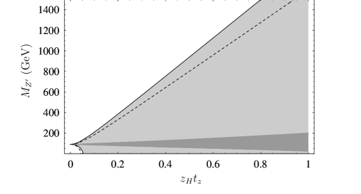
Figure 1: Bounds at the $95\%$ confidence level in the $(z_{H}t_{z},M_{Z^{\prime}})$ plane, where $z_{H}t_{z}=z_{H}g_{z}/g$ is the ratio of the $U(1)_{z}$-coupling of the Higgs doublet to the weak coupling. Electromagnetic strength corresponds to $z_{H}t_{z}\simeq 0.48$. The limit $z_{H}t_{z}\rightarrow 0$ represents either an extremely weakly coupled new boson, or a model with $z\propto B-L$. The disallowed region due to the bound on the $T$ parameter for $M_{H}=115$ GeV is shaded light gray. The dotted line shows the shift in the bound for $M_{H}=300$ GeV. Here we have used $T=-0.02\pm 0.13(+0.09)$, where the central value corresponds to $M_{H}=115$ GeV and the shift (in parentheses) to $M_{H}=300$ GeV [1].

Finally, we observe that a simple relation exists among the mixing angle $\theta^{\prime}$ (given by Eq. (2.5)), $M_{Z^{\prime}}$, and $T$:

$$\alpha T=\sin^{2}\theta^{\prime}\left(\frac{M_{Z^{\prime}}^{2}}{M_{Z}^{2}}-1\right).~{}$$ (4.17)

Note that if the Higgs doublet is uncharged under $U(1)_{z}$ (and so $T=0$), then $\theta^{\prime}=0$ and the $Z$ has no anomalous couplings at tree level. From this expression, it can be seen that through most of the region of Fig. 1 allowed by the experimental constraints on $T$,  $\theta^{\prime}\ll 1$.

4.3 Anomalous $Z$ couplings

We next analyze the tree-level couplings of the neutral gauge bosons to matter. In terms of the mass eigenstates, the interaction takes the form

$${\cal L}_{Z,Z^{\prime}}=\frac{g}{\cos\theta_{w}}\sum_{f}\overline{f}~{}\gamma^{\mu}\left(c_{f}\;,\;c^{\prime}_{f}\right)\left(\begin{array}[]{cc}\cos\theta^{\prime}&-\sin\theta^{\prime}\\ \sin\theta^{\prime}&\cos\theta^{\prime}\\ \end{array}\right)\left(\begin{array}[]{c}Z_{\mu}\\ Z^{\prime}_{\mu}\\ \end{array}\right)f~{},$$ (4.18)

where $f$ ranges over the chiral fields $u^{i}_{L}$, $d^{i}_{L}$, $u^{i}_{R}$, $d^{i}_{R}$, $\nu^{i}_{L}$, $e^{i}_{L}$, $e^{i}_{R}$, and $\nu^{k}_{R}$. The couplings $c_{f}$ and $c^{\prime}_{f}$ are given by

$$c_{f} = T^{3}_{f}-q_{f}\sin^{2}\theta_{w}$$

$$c^{\prime}_{f} = z_{f}t_{z}\cos\theta_{w}/2,$$ (4.19)

where $Y_{f}$ and $z_{f}$ are the hypercharge and $U(1)_{z}$ charge of fermion $f$ (see Table 1), while $T^{3}_{f}$ and $q_{f}$ are its weak isospin and electric charge, which satisfy $q_{f}=T^{3}_{f}+Y_{f}/2$. Since the couplings of the $Z$ to matter are known so precisely, the constraint $\theta^{\prime}\ll 1$ must hold.

In the standard model, electroweak physics is conveniently described in terms of the electromagnetic coupling, the Fermi constant, and the physical $Z$ mass (in addition to the particle masses and CKM matrix elements). Following this convention, we focus on ${\cal L}_{Z}$ from Eq. (4.18) and reexpress it in terms of these parameters by way of defining a new, physical weak angle $\theta_{W}$ such that

$$\frac{G_{F}}{\sqrt{2}}\equiv\frac{\pi\alpha(M_{Z})}{2\sin^{2}\theta_{W}\cos^{2}\theta_{W}M_{Z}^{2}}~{},$$ (4.20)

where $\alpha(M_{Z})$ is the fine-structure constant defined at the $Z$ mass [$\alpha(M_{Z})^{-1}=128.92\pm 0.03$]. For our effective theory at tree level, the relation between $\theta_{w}$ and $\theta_{W}$ is given by

$$\sin^{2}\theta_{W}\cos^{2}\theta_{W}=\sin^{2}\theta_{w}\cos^{2}\theta_{w}(1+\alpha T)~{}.$$ (4.21)

Keeping terms to first order in $\alpha T$ and to order $\theta^{\prime 2}$, the interaction of the $Z$ with matter may now be written as

$${\cal L}_{Z}=\frac{e}{\sin\theta_{W}\cos\theta_{W}}\left[1+\frac{1}{2}(\alpha T-\theta^{\prime 2})\right]\sum_{f}\bar{f}\gamma^{\mu}(g_{f}+\delta g_{f})fZ_{\mu}~{},$$ (4.22)

where terms of order $\alpha T\,\delta g_{f}$ and $\theta^{\prime 2}\,\delta g_{f}$ are discarded. Here $e$ is the electromagnetic gauge coupling, and $g_{f}$ and $\delta g_{f}$ are given by

$$g_{f} = T^{3}_{f}-q_{f}\sin^{2}\theta_{W}$$

$$\delta g_{f} = q_{f}\alpha T\frac{\sin^{2}\theta_{W}\cos^{2}\theta_{W}}{\cos^{2}\theta_{W}-\sin^{2}\theta_{W}}+z_{f}t_{z}\cos\theta_{W}\frac{\theta^{\prime}}{2}~{}.$$ (4.23)

In the limit $M_{Z}\ll M_{Z^{\prime}}$ the term of order $\theta^{\prime 2}$ is suppressed relative to the others, but in general, and particularly for $Z^{\prime}$ very light compared to $Z$, it can happen that $\theta^{\prime 2}\sim\alpha T$ [see Eq. (4.17)].

Using Eqs. (4.22) and (4.23), any measurable quantity depending on the $Z$-pole coupling to matter may be expressed (at tree-level) in terms of $M_{Z}/M_{Z^{\prime}}$ and two couplings which we take to be $z_{q}t_{z}$ and $z_{H}t_{z}$. Having expressed ${\cal L}_{Z}$ in terms of the physical weak angle $\theta_{W}$, the prediction for the new theory will be the radiatively-corrected standard model prediction, plus a small shift due to new physics that depends on the parameters $M_{Z^{\prime}}$, $z_{H}t_{z}$, and $z_{q}t_{z}$.

A precise bound in the $Z^{\prime}$ parameter space can be obtained by performing a global fit to all the electroweak data. However, in order to understand the dependence of the observables on the $Z^{\prime}$ parameters, we restrict attention here to two well-measured, representative $Z$-pole observables, in addition to the $T$ parameter: the total decay width of the $Z$ boson, $\Gamma_{Z}$, and the left-right asymmetry of the electron. We expect that the bounds derived this way will not be substantially different than those set by a global fit.

The current experimental value of $\Gamma_{Z}$, $2.4952\pm 0.0023$ GeV, is in excellent agreement with the standard model prediction of $2.4966\pm 0.0016$ GeV [1]. The change in the $Z$ couplings due to the presence of the $Z^{\prime}$ boson leads to a shift in $\Gamma_{Z}$, resulting in the bound shown in Fig. 2. Since we are interested in comparing bounds on the parameters $M_{Z^{\prime}}$, $z_{q}t_{z}$, and $z_{H}t_{z}$ to those from the $T$ parameter, we show bounds for a given value of $z_{q}t_{z}$ as contours in the $(z_{H}t_{z},M_{Z^{\prime}})$ plane. To understand the qualitative features of Fig. 2, it is helpful to consider the limit $M_{Z}^{\prime}\gg M_{Z}$, which is reliable over much of the vertical range, in which case $\Gamma_{Z}$ takes the simple form

$$\Gamma_{Z}=\Gamma_{Z}^{\it SM}\left[1+(0.55z_{H}^{2}-1.29z_{H}z_{q})t_{z}^{2}M_{Z}^{2}/M_{Z^{\prime}}^{2}+\mathcal{O}\left(M_{Z}^{4}/M_{Z^{\prime}}^{4}\right)\right],$$ (4.24)

where $\Gamma_{Z}^{\it SM}$ is the current standard model value for the total width. For $z_{H}$ large relative to $z_{q}$ (the $U(1)_{R}$ limit), Eq. (4.24) implies that the bound on $M_{Z^{\prime}}$ grows linearly with $z_{H}t_{z}$, with a slope of roughly $2$ TeV per unit $z_{H}t_{z}$. In the limit where $z_{q}$ is large relative to $z_{H}$ (the $z\propto B-L$ limit) the bound grows as $\sqrt{z_{H}t_{z}}$. These features are reflected in Fig. 2. We note that for $z_{H}t_{z}\ll 1$ there is an allowed region of parameter space with $M_{Z^{\prime}}<M_{Z}$.

Fig. 2 shows that the bounds from $\Gamma_{Z}$ depend on the magnitude of the coupling $z_{q}t_{z}$, as well as its sign relative to $z_{H}t_{z}$ which we have taken to be positive. For $z_{H}t_{z}$ and $z_{q}t_{z}$ of electromagnetic strength, i.e., $z_{H}t_{z}=\sin\theta_{w}$, $z_{q}t_{z}=\pm\sin\theta_{w}/3$, the $T$-parameter bound is $M_{Z^{\prime}}>0.9$ TeV, while the $\Gamma_{Z}$-bound is significantly weaker if $z_{H}t_{z}$ and $z_{q}t_{z}$ are of the same sign. If they are of opposite sign the bound from $\Gamma_{Z}$ is stronger than that from $T$, with $M_{Z^{\prime}}>1.2$ TeV. For sufficiently small $z_{H}t_{z}$ the $\Gamma_{Z}$-bound is always stronger than the $T$-parameter bound (and both vanish at tree level in the $z_{H}t_{z}\rightarrow 0$ limit).

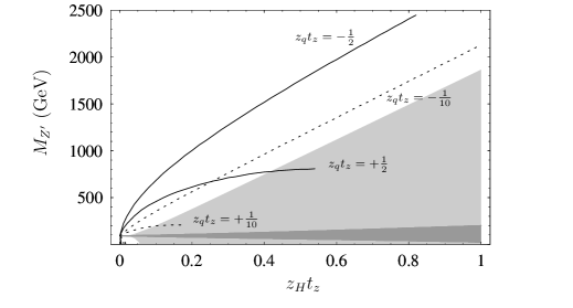
Figure 2: Bounds from precision measurements of the total $Z$ width at the $95\%$ confidence level plotted as contours in the $(z_{H}t_{z},M_{Z^{\prime}})$ plane, for $z_{q}t_{z}=\pm\frac{1}{10},\pm\frac{1}{2}$. In each case the allowed region is to the left of the line. Included in gray are bounds from $T$ for $M_{H}=115$ GeV.  

We have also examined bounds coming from the left-right asymmetry of the electron, $A_{e}$. The experimental value, from the angular distribution of the $\tau$ polarization [1], is $0.1498\pm 0.0048$; the standard model predicts $0.1478\pm 0.0012$. An expression analogous to Eq. (4.24) can be derived for $A_{e}$,

$$A_{e}=A_{e}^{\it SM}\left[1+(24z_{H}^{2}+60z_{H}z_{q})t_{z}^{2}M_{Z}^{2}/M_{Z^{\prime}}^{2}+\mathcal{O}\left(M_{Z}^{4}/M_{Z^{\prime}}^{4}\right)\right].$$ (4.25)

We find that the bounds from $A_{e}$ are complementary to those from $\Gamma_{Z}$: the former are comparable with the latter for opposite signs of $z_{q}t_{z}$ (this fact is suggested by Eqs. (4.24) and (4.25)). For $z_{H}t_{z}$ and $z_{q}t_{z}$ of electromagnetic strength, and of the same sign, one finds that the bound from $A_{e}$ is $M_{Z^{\prime}}>1.0$ TeV at the 95% confidence level.

In summary, $M_{Z^{\prime}}>{\cal O}(1)$ TeV in models with $z_{H}t_{z}$ and $z_{q}t_{z}$ of electromagnetic strength.

5 Conclusions

Our study of new color-singlet and electrically neutral gauge bosons shows that there remain many possibilities to explore even in the simplest extensions of the standard model. We have first demonstrated that the $SU(3)_{C}\times SU(2)_{W}\times U(1)_{a}\times U(1)_{b}$ gauge group is consistent with the measured electric charges of the observed fermions only if it is equivalent to the $SU(3)_{C}\times SU(2)_{W}\times U(1)_{Y}\times U(1)_{z}$ gauge group, where $U(1)_{Y}$ is the standard model hypercharge, and $U(1)_{z}$ is a new gauge group in a kinetically-diagonal basis. Symmetry breaking is described, without loss of generality for the purposes of this paper, by the usual doublet Higgs along with a single complex scalar, whose $U(1)_{z}$ charge is +1.

We have then concentrated on the case where the $U(1)_{z}$ symmetry is non-anomalous, the $U(1)_{z}$ charges of the observed fermions are generation independent, and any new fermions are singlets under $SU(3)_{C}\times SU(2)_{W}\times U(1)_{Y}$. We allow for an arbitrary number of right-handed neutrinos charged under $U(1)_{z}$. As long as there are at least three right-handed neutrinos, a continuous family of $U(1)_{z}$-charge assignments is consistent with both anomaly cancellation and the existence of fermion masses. The $U(1)_{z}$-charges of the observed fermions depend on two parameters, chosen to be the charges $z_{q}$ and $z_{u}$ of the left-handed quark doublets and right-handed up-type quarks. The $U(1)_{z}$ charge of the Higgs doublet has to be given by $z_{H}=z_{u}-z_{q}$ in order to allow the existence of the top Yukawa coupling. Although the $U(1)_{z}$ charges of the right-handed neutrinos are not uniquely determined, the anomaly cancellation conditions allow only a limited set of charge assignments. Moreover, each of these right-handed neutrino charge assignments implies a different set of higher-dimensional operators that could generate the neutrino masses. As a byproduct, it is possible to obtain viable neutrino mass matrices even when all the higher-dimensional operators have coefficients of order unity.

Some fermion charge assignments correspond to relatively simple relations between $z_{q}$ and $z_{u}$. Among them are several of the popular models in the literature, as well as other simple charge assignments that, to the best of our knowledge, have not been analyzed before. In fact, in a general effective field theory arising from unspecified underlying dynamics, and involving renormalization-group running from the fundamental scale to that of the effective theory, there may be no good reason to choose a particular relation among the charges. On the other hand, if the gauge coupling is sufficiently small, then the renormalization-group running may be ignored. Furthermore, various theoretical developments within the last few years have demonstrated that the range of possibilities for physics at a fundamental scale is very wide, and hence it is reasonable to consider charge assignments that are different than those arising from traditional grand unified theories.

An example that is both simple and instructive is based on the $SU(3)_{C}\times SU(2)_{W}\times U(1)_{Y}\times U(1)_{B-L}$ gauge group. As we discussed in Section 4.1, in this case there is no tree-level mixing between the $Z$ and $Z^{\prime}\equiv Z_{B-L}$ bosons, because $z_{H}=0$. The best limits on the mass and coupling of the $Z_{B-L}$ boson is then set by the searches for direct $Z^{\prime}$ production in experiments at the Tevatron and LEPII. For a $Z_{B-L}$ coupling to quarks and leptons of electromagnetic strength, the lower mass limit set by searches at CDF is around 480 GeV. We reiterate though that the gauge coupling is a free parameter that could be substantially smaller than the electromagnetic gauge coupling. If that is the case, then the Tevatron mass limits no longer apply, and the best bounds for a $Z_{B-L}$ of mass below 200 GeV are set at LEP. With the exception of a few narrow mass intervals around the center-of-mass energies where the integrated luminosity is large, a $Z_{B-L}$ coupling to leptons as large as $10^{-2}$ would suffice to hide the narrow resonance from the LEP experiments.

For generic charge assignments with $z_{H}\neq 0$, the strongest bounds on the $Z^{\prime}$ parameters come from precision measurements at the $Z$-pole. The presence of the new $Z^{\prime}$ in general induces at the tree-level both a shift in the $Z$ mass (expressed in terms of the $T$ parameter) and a shift in its couplings from the standard model values. For a $Z^{\prime}$ coupling to fermions of typical electromagnetic strength, we estimate the lower bound on the mass $M_{Z^{\prime}}$ of the $Z^{\prime}$ to be roughly in the $0.9-1.2$ TeV range. As the $Z^{\prime}$ coupling to the Higgs doublet weakens, the lower bound on $M_{Z^{\prime}}$ from the indirect, $Z$-pole studies drops significantly (see Fig. 2).

We emphasize that we have studied so far only the “tip of the iceberg”. There are many avenues for research related to new gauge bosons. It would be interesting to investigate systematically the possible charge assignments and limits on couplings when the $U(1)_{z}$ charges are generation dependent (various examples of this type have been analyzed recently in Ref. [25]). Furthermore, our simplifying assumption that there are no “exotic” fermions charged under the standard model group could be dropped. Given that the scale of new physics is expected to be at the TeV scale, one could also consider an anomalous $U(1)_{z}$. Experimental limits on the parameter space associated with the gauge bosons in each of these generalizations need to be derived. In fact, only few dedicated searches for light narrow resonances have been performed, and therefore there is a possibility that the signal for a new gauge boson already exists in the current data.

Acknowledgements: We would like to thank Sekhar Chivukula, Stephen Martin, Rabi Mohapatra, Maurizio Piai and German Valencia for helpful comments. This work was supported in part by grant DE-FG02-92ER-4074. Fermilab is operated by University Research Association, Inc., under contract DE-AC02-76CH03000.

References

- [1] K. Hagiwara et al. [Particle Data Group Collaboration], “Review Of Particle Physics,” Phys. Rev. D 66, 010001 (2002).
-
[2]
For a review, see
J. L. Hewett and T. G. Rizzo, “Low-Energy Phenomenology Of Superstring
Inspired E(6) Models,”
Phys. Rept. 183, 193 (1989);
M. Cvetic and P. Langacker, “Implications of Abelian Extended Gauge Structures From String Models,” Phys. Rev. D 54, 3570 (1996) [arXiv:hep-ph/9511378]. - [3] For a review, see C. T. Hill and E. H. Simmons, “Strong dynamics and electroweak symmetry breaking,” arXiv:hep-ph/0203079.
- [4] J. Erler and P. Langacker, “Indications for an extra neutral gauge boson in electroweak precision data,” Phys. Rev. Lett. 84, 212 (2000) [arXiv:hep-ph/9910315].
- [5] E. Jenkins, “Searching For A (B-L) Gauge Boson In P Anti-P Collisions,” Phys. Lett. B 192, 219 (1987).
- [6] For a review, see A. Leike, “The phenomenology of extra neutral gauge bosons,” Phys. Rept. 317, 143 (1999) [arXiv:hep-ph/9805494].
-
[7]
P. Galison and A. Manohar, “Two Z’s Or Not Two Z’s?,” Phys. Lett. B 136, 279 (1984);
F. del Aguila, M. Masip and M. Perez-Victoria, “Physical parameters and renormalization of U(1)-a x U(1)-b models,” Nucl. Phys. B 456, 531 (1995) [arXiv:hep-ph/9507455]. - [8] K. S. Babu, C. Kolda and J. March-Russell, “Implications of generalized Z Z’ mixing,” Phys. Rev. D 57, 6788 (1998) [arXiv:hep-ph/9710441].
- [9] S. Weinberg, “The Quantum Theory Of Fields. Vol. 2: Modern Applications,” Cambridge, UK: Univ. Pr. (1996), p.388.
- [10] For a review, see R. N. Mohapatra, “Unification And Supersymmetry. The Frontiers Of Quark - Lepton Physics,” Berlin, Germany: Springer ( 1986) 309 P. ( Contemporary Physics).
- [11] V. D. Barger and R. J. Phillips, “Collider Physics,” Addison-Wesley (1987), p. 115.
- [12] S. L. Wu, “E+ E- Physics At Petra: The First 5-Years,” Phys. Rept. 107, 59 (1984).
- [13] G. Abbiendi et al. [OPAL Collaboration], “Tests of the standard model and constraints on new physics from measurements of fermion pair production at 189-GeV at LEP,” Eur. Phys. J. C 13, 553 (2000) [arXiv:hep-ex/9908008].
- [14] P. Abreu et al. [DELPHI Collaboration], “Measurement and Interpretation of Fermion-Pair Production at LEP Energies of 183 and 189 GeV,” Phys. Lett. B 485, 45 (2000) [arXiv:hep-ex/0103025].
- [15] M. Acciarri et al. [L3 Collaboration], “Search for manifestations of new physics in fermion pair production at LEP,” Phys. Lett. B 489, 81 (2000) [arXiv:hep-ex/0005028].
- [16] F. A. Berends, R. Kleiss and S. Jadach, “Radiative Corrections To Muon Pair And Quark Pair Production In Electron - Positron Collisions In The Z(0) Region,” Nucl. Phys. B 202, 63 (1982).
- [17] A. Blondel et al. [LEP Energy Working Group Collaboration], “Evaluation of the LEP centre-of-mass energy above the W pair production threshold,” Eur. Phys. J. C 11, 573 (1999) [Eur. Phys. J. C 11, 729 (1999)] [arXiv:hep-ex/9901002].
- [18] E. D. Carlson, “Limits On A New U(1) Coupling,” Nucl. Phys. B 286, 378 (1987).
- [19] R. Barate et al. [ALEPH Collaboration], “Study of fermion pair production in e+ e- collisions at 130-GeV to 183-GeV,” Eur. Phys. J. C 12, 183 (2000) [arXiv:hep-ex/9904011].
- [20] F. Abe et al. [CDF Collaboration], “Search for new gauge bosons decaying into dileptons in anti-p p collisions at s**(1/2) = 1.8-TeV,” Phys. Rev. Lett. 79, 2192 (1997).
- [21] S. Abachi et al. [D0 Collaboration], “Search for additional neutral gauge bosons,” Phys. Lett. B 385, 471 (1996).
- [22] F. Abe et al. [CDF Collaboration], “A Search for new gauge bosons in anti-p p collisions at S**(1/2) = 1.8-TeV,” Phys. Rev. Lett. 68, 1463 (1992).
- [23] F. Abe et al. [CDF Collaboration], “Search for new gauge bosons decaying into dielectrons in anti-p p collisions at s**(1/2) 1.8-TeV,” Phys. Rev. D 51, 949 (1995).
- [24] C. P. Burgess, S. Godfrey, H. Konig, D. London and I. Maksymyk, “Model independent global constraints on new physics,” Phys. Rev. D 49, 6115 (1994) [arXiv:hep-ph/9312291].
- [25] R. S. Chivukula and E. H. Simmons, “Electroweak limits on non-universal Z’ bosons,” Phys. Rev. D 66, 015006 (2002) [arXiv:hep-ph/0205064].