Hard exclusive baryon-antibaryon production
in two-photon collisions

Abstract

We study baryon pair production in two-photon collisions, $\gamma\gamma\rightarrow B\bar{B}$, within perturbative quantum chromodynamics, treating baryons as quark-diquark systems. We extend previous work within the same approach by treating constituent-mass effects systematically by means of an expansion in the small parameter (mass/photon energy). Our approach enables us to give a consistent description of the cross sections for all octet baryon channels. Adopting the model parameters from foregoing work, we are able to reproduce the most recent large-momentum-transfer data from LEP for the $p\bar{p}$, $\Lambda\bar{\Lambda}$, and $\Sigma^{0}\bar{\Sigma}^{0}$ channels in a quite satisfactory way. We also briefly address the crossed process for the proton channel, $\gamma p\rightarrow\gamma p$.

1 Introduction

Theoretical analyses of exclusive reactions in quantum chromodynamics (QCD), where intact hadrons appear in the initial and final states, are of great importance for a better understanding of the mechanism of confinement and of the dynamics of hadronic bound states. Although much progress has been made in the theoretical understanding within frameworks based on perturbation theory blrev ; pire ; stefanis , there still remain many open problems. It is a matter of ongoing discussion whether the currently experimentally accessible energies are high enough such that the perturbative treatment becomes applicable contro . As a possible way to model non-perturbative effects which do not seem to be fully separated from perturbatively calculable contributions at intermediately large momentum transfers, the introduction of diquarks has been proposed in anskrollpire . In a series of papers this effective model has been developed further and successfully applied to a variety of exclusive reactions gamgampp ; Compton ; fixed ; time ; Ja94 ; KSG96 ; KSPS97 ; fizb ; CW ; mass . In this work we continue the investigations within the diquark model and consider exclusive two-photon reactions.

The theoretical description of exclusive reactions within perturbation theory is based on the ideas of Brodsky and Lepage blrev ; blpaper , and Efremov and Radyushkin efrad . Within this so-called hard scattering picture (HSP), an exclusive reaction amplitude can be written as a convolution of process-dependent, perturbatively calculable, hard-scattering amplitudes with process-independent probability amplitudes for finding the pertinent valence Fock states in the scattering hadrons. The latter are non-perturbative quantities, but their dependence on the momentum-transfer $Q^{2}$ can be determined perturbatively. Their extraction from experimental observations is challenged by the fact that they enter only integrated quantities, such as form factors. However, their shape can be constrained with the help of QCD sum rules, lattice QCD and other non-perturbative methods. These studies seem to indicate that the distribution of longitudinal momentum fractions among the valence quarks in a nucleon is quite asymmetric for finite momentum transfers. This can be interpreted as evidence for binding effects between two quarks in a nucleon and motivates the introduction of diquarks stefanis ; anselmino . Comprehensive reviews of the HSP are given, for example, in blrev ; pire ; stefanis .

The HSP as presented above is exactly valid only for asymptotically large momentum transfers, $Q^{2}\rightarrow\infty$, where long- and short-distance effects are completely incoherent. However, as already mentioned above, experimental observations seem to indicate that this separation is not yet achieved at presently accessible momentum transfers of a few GeV. Thus a perturbative calculation of the short distance contributions may not be completely self-consistent.

Inspired by the aforementioned correlations observed in hadronic wave functions, a quark-diquark model was developed in anskrollpire to parameterize possible non-perturbative effects within a perturbative framework. Within this model which is based on the HSP, baryons are treated as quark-diquark systems. The composite nature of the diquarks is taken into account by diquark form factors which are parameterized such that asymptotically the scaling behavior of the pure quark HSP emerges. The possibility of the reformulation of the pure quark HSP in terms of quark and diquark degrees of freedom has been demonstrated in bernd ; marc . In earlier studies of two-photon annihilation into baryons, $\gamma\gamma\rightarrow B\bar{B}$ gamgampp , and of Compton scattering off baryons, $\gamma B\rightarrow\gamma B$ Compton ; KSG96 , all quark masses have been neglected, while masses for diquarks were introduced as additional parameters. In recent studies within the diquark model fizb ; CW ; mass a different strategy was adopted to treat mass effects more consistently without introducing new mass parameters for the hadronic constituents. In the following we will reconsider the two-photon reactions with this improved treatment of mass effects.

We start by introducing the necessary ingredients of the diquark model for the reaction $\gamma\gamma\rightarrow B\bar{B}$. While we try to keep the present discussion as self-contained as possible, we omit certain details of the model which can be found, for example, in CW . We explain our choice of quark and diquark distribution amplitudes (DAs), and our treatment of constituent masses in Sections 2.1 and 2.2, respectively. Having collected all ingredients of the model, we list our analytical results for the hard scattering amplitudes for the two-photon annihilation process in Section 2.3. In Section 3 we present the numerical results for this reaction, compare to existing data for the proton-antiproton, $\Lambda\bar{\Lambda}$, and $\Sigma^{0}\bar{\Sigma}^{0}$ channels, and give predictions for other final states. We then go on and briefly comment on the crossed reaction, specifically Compton scattering off protons. Section 5 ends the discussion with a summary and some concluding remarks.

2 The $\gamma\gamma\rightarrow B\bar{B}$ amplitude

As stated in the introduction, within the HSP an exclusive scattering amplitude can be written as a convolution integral of a hard-scattering amplitude with distribution amplitudes, describing the longitudinal momentum distribution of valence quarks in the participating hadrons. In the diquark model a baryon is considered as consisting of a quark and a diquark. The diquark is treated as a quasi-elementary constituent which may survive medium hard collisions.

Within this framework, we obtain the following convolution integral for the $\gamma\gamma\rightarrow B\bar{B}$ amplitude:

$$\mathcal{M}_{\{\lambda\}}\left(\hat{s},\hat{t}\right) = \int\limits_{0}^{1}dx_{1}\int\limits_{0}^{1}dy_{1}\Psi_{B}^{\dagger}\left(x_{1}\right)\Psi_{\bar{B}}^{\dagger}\left(y_{1}\right)$$ (1)

$$\times \hat{T}_{\{\lambda\}}\left(x_{1},y_{1};\hat{s},\hat{t}\right),$$

where we have suppressed Lorentz and color indices in the convolution integral. Here $\hat{T}$ is the process-dependent hard-scattering amplitude for producing a quark-antiquark and a diquark-antidiquark pair in a two-photon collision. In the notation used above, the quark and the antiquark carry momentum fractions $x_{1}$ in the baryon, and $y_{1}$ in the antibaryon, while the diquark and antidiquark carry momentum fractions $x_{2}=1-x_{1}$ and $y_{2}=1-y_{1}$, respectively ($0\leq x_{i},\,y_{i}\leq 1$). $\hat{T}$ consists of all possible tree diagrams contributing to the elementary scattering process $\gamma\gamma\rightarrow qD\bar{q}\bar{D}$, where the momenta of all constituents (quarks $q$ and diquarks $D$) are collinear to those of their parent hadrons. The distribution amplitudes $\Psi_{B}$ are process-independent probability amplitudes for finding the pertinent valence Fock states in the baryon $B$ with the constituents carrying the longitudinal momentum fractions $x_{i},\,y_{i}$ of the parent baryon and being collinear up to the (factorization) scale $\tilde{p}_{\perp}$. In (1) we have already neglected the (logarithmic) $\tilde{p}_{\perp}$ dependence, since this dependence is only of minor importance in the restricted kinematic range of intermediately large momentum transfer we are considering in this work. For convenience, we use massless Mandelstam variables $\hat{s},\,\hat{t}$, and $\hat{u}$, rather than the usual (massive) ones, $s,\,t$, and $u$. The subscript ${\{\lambda\}}$ denotes all possible configurations of photon and baryon helicities.

For the process $\gamma\gamma\rightarrow B\bar{B}$, there are six independent complex helicity amplitudes $\mathcal{M}_{\lambda_{\bar{B}},\,\lambda_{B};\,\lambda_{1},\,\lambda_{2}}$, where the $\lambda_{i},\,i=1,2$ label the helicities of the incoming photons, and $\lambda_{B},\,\lambda_{\bar{B}}$ are the helicities of the baryon and antibaryon, respectively. Following the conventions in rosti76 , we express our observables in terms of the following amplitudes:

$$\overline{\phi}_{1} = \mathcal{M}_{-\frac{1}{2},\,\frac{1}{2};\,1,\,-1},$$

$$\overline{\phi}_{2} = \mathcal{M}_{-\frac{1}{2},\,-\frac{1}{2};\,1,\,1},$$

$$\overline{\phi}_{3} = \mathcal{M}_{-\frac{1}{2},\,\frac{1}{2};\,1,\,1},$$

$$\overline{\phi}_{4} = \mathcal{M}_{-\frac{1}{2},\,-\frac{1}{2};\,1,\,-1},$$

$$\overline{\phi}_{5} = \mathcal{M}_{\frac{1}{2},\,-\frac{1}{2};\,1,\,-1},$$

$$\overline{\phi}_{6} = \mathcal{M}_{\frac{1}{2},\,\frac{1}{2};\,1,\,1}.$$ (2)

The remaining helicity configurations are related to these via parity and time reversal invariance. We normalize these helicity amplitudes such that the differential cross section for two-photon annihilation into a baryon-antibaryon pair is given by

$$\frac{d\sigma}{dt} = \frac{1}{32\pi s^{2}}\left[\left|\overline{\phi}_{1}\right|^{2}+\left|\overline{\phi}_{2}\right|^{2}+2\left|\overline{\phi}_{3}\right|^{2}\right.$$ (3)

$$\quad\quad+\left.2\left|\overline{\phi}_{4}\right|^{2}+\left|\overline{\phi}_{5}\right|^{2}+\left|\overline{\phi}_{6}\right|^{2}\right].$$

Within the HSP constituent masses are usually neglected. We relate constituent masses to the pertinent baryon mass when calculating the hard-scattering amplitude. By a subsequent expansion in powers of $(m_{B}/\sqrt{\hat{s}})$, where $m_{B}$ denotes the baryon mass, we obtain the leading mass-correction terms. We will elaborate more on our treatment of mass effects in Section 2.2.

2.1 Baryons as quark-diquark systems

In the ground state diquarks have positive parity and either spin 0 (scalar diquarks $S$) or spin 1 (vector diquarks $V$). Because vector diquarks are mainly responsible for spin flips they are essential to describe spin effects.

Neglecting transverse momentum, we can write the baryon wave function in a covariant way so that only baryonic quantities (momentum $p_{B}$, helicity $\lambda$, baryon mass $m_{B}$) appear. For the lowest-lying baryon octet, assuming zero relative orbital angular momentum between quark and diquark, the wave function (already integrated over transverse momenta) can be written as

$$\Psi_{B}(p_{B},x,\lambda) = f_{S}^{B}\Psi_{S}^{B}(x)\chi_{S}^{B}\,u(p_{B},\lambda)$$

$$+ f_{V}^{B}\Psi_{V}^{B}(x)\chi_{V}^{B}\frac{1}{\sqrt{3}}\left(\gamma^{\alpha}+\frac{p_{B}^{\alpha}}{m_{B}}\right)\gamma_{5}\,u(p_{B},\lambda).$$

Here the $\chi_{D}^{B}$ are SU(3) quark-diquark flavor wave functions, and the two functions $\Psi_{S}$ and $\Psi_{V}$, for scalar and vector diquarks, respectively, represent the nonperturbative probability amplitudes for finding these constituents in the baryon. The notation in Eq. (2.1) is slightly sloppy, the open index in the vector part of the wave function corresponds to the Lorentz index of the V-diquark polarization vector and is contracted appropriately in the convolution integral, Eq. (1). The constants $f_{D}^{B}$ may be interpreted as baryon decay constants. The wave function for antibaryons is given by

$$\Psi_{\bar{B}}(p_{\bar{B}},x,\lambda) = f_{S}^{B}\Psi_{S}^{B}(x)\chi_{S}^{\bar{B}}\,v(p_{\bar{B}},\lambda)$$

$$+ f_{V}^{B}\Psi_{V}^{B}(x)\chi_{V}^{\bar{B}}\frac{1}{\sqrt{3}}\left(\gamma^{\alpha}-\frac{p_{\bar{B}}^{\alpha}}{m_{\bar{B}}}\right)\gamma_{5}\,v(p_{\bar{B}},\lambda),$$

where we have used charge  conjugation  $v(p,\lambda)=i\gamma^{2}$ $u^{*}(p,\lambda)$.

In the following we will use a quark-diquark distribution amplitude of the form huang

$$\Psi_{D}^{B}(x) = N^{B}x(1-x)^{3}(1+c_{1}x+c_{2}x^{2})$$ (6)

$$\qquad\qquad\quad\;\exp\left\{-b^{2}\left(\frac{m_{q}^{2}}{x}+\frac{m_{D}^{2}}{1-x}\right)\right\},$$

where $c_{i}=0$ for scalar diquarks. This DA for octet baryons $B$ has been successfully used in previous applications of the diquark-model fixed ; time ; Ja94 ; KSG96 ; KSPS97 ; fizb ; CW ; mass . It is an adaptation of a meson DA, obtained by transforming a harmonic oscillator wave function to the light cone. Therefore, the masses appearing in the exponent are constituent masses. The oscillator parameter $b$ is fixed by the requirement that the mean intrinsic transverse momentum of quarks inside the baryon $B$ is $\sqrt{\left<k_{T}^{2}\right>}\approx$ 600 MeV. This value was found experimentally by the EMC collaboration in semi-inclusive deep inelastic $\mu p$ scattering EMC . Theoretical considerations also indicate a value of this magnitude sterman . Furthermore, the exponent suppresses contributions from the endpoint regions $x\rightarrow 0,1$ in the convolution integral (1). Endpoint-damping Sudakov-type exponents generally arise when resumming corrections from soft gluon radiation blpaper ; sudakov . The exponent in (6) could be interpreted as simulating this Sudakov suppression effect in the endpoint region. The normalization constant $N^{B}$ in Eq. (6) is fixed by the requirement that

$$\int\limits_{0}^{1}\Psi_{D}(x)dx=1.$$ (7)

The SU(3) quark-diquark flavor wave functions $\chi_{S}^{D}$ for the lowest-lying baryon octet are listed in Table 1.

Table 1: SU(3) quark-diquark flavor wave functions for the lowest lying baryon octet

$$\begin{array}[]{l@{\hspace*{2mm}}l}\hline\cr\vskip 3.0pt plus 1.0pt minus 1.0pt\cr\chi_{S}^{p}=uS_{[u,d]}\hfil\hskip 5.69054pt&\chi_{V}^{p}=\frac{\scriptstyle 1}{\scriptstyle\sqrt{3}}\left[uV_{\{u,d\}}-\sqrt{2}dV_{\{u,u\}}\right]\\ \chi_{S}^{n}=dS_{[u,d]}\hfil\hskip 5.69054pt&\chi_{V}^{n}=-\frac{\scriptstyle 1}{\scriptstyle\sqrt{3}}\left[dV_{\{u,d\}}-\sqrt{2}uV_{\{d,d\}}\right]\\ \chi_{S}^{\Sigma^{+}}\!\!\!=-uS_{[u,s]}\hfil\hskip 5.69054pt&\chi_{V}^{\Sigma^{+}}=\frac{\scriptstyle 1}{\scriptstyle\sqrt{3}}\left[uV_{\{u,s\}}-\sqrt{2}sV_{\{u,u\}}\right]\\ \chi_{S}^{\Sigma^{0}}\!\!\!\!=\!\!\frac{\scriptstyle 1}{\scriptstyle\sqrt{2}}\left[dS_{[u,s]}+uS_{[d,s]}\right]\hfil\hskip 5.69054pt&\chi_{V}^{\Sigma^{0}}=\frac{\scriptstyle 1}{\scriptstyle\sqrt{6}}\left[2sV_{\{u,d\}}-dV_{\{u,s\}}\right.\\ \hfil\hskip 5.69054pt&\qquad\quad\left.-uV_{\{d,s\}}\right]\\ \chi_{S}^{\Sigma^{-}}\!\!\!=dS_{[d,s]}\hfil\hskip 5.69054pt&\chi_{V}^{\Sigma^{-}}=-\frac{\scriptstyle 1}{\scriptstyle\sqrt{3}}\left[dV_{\{d,s\}}-\sqrt{2}sV_{\{d,d\}}\right]\\ \chi_{S}^{\Lambda}=\frac{\scriptstyle 1}{\scriptstyle\sqrt{6}}\left[uS_{[d,s]}-dS_{[u,s]}\right.\hfil\hskip 5.69054pt&\chi_{V}^{\Lambda}\!=\!\frac{\scriptstyle 1}{\scriptstyle\sqrt{2}}\left[uV_{\{d,s\}}-dV_{\{u,s\}}\right]\\ \qquad\qquad\left.\,-2sS_{[u,d]}\right]\hfil\hskip 5.69054pt&\\ \chi_{S}^{\Xi^{0}}\!\!\!=sS_{[u,s]}\hfil\hskip 5.69054pt&\chi_{V}^{\Xi^{0}}=-\frac{\scriptstyle 1}{\scriptstyle\sqrt{3}}\left[sV_{\{u,s\}}-\sqrt{2}uV_{\{s,s\}}\right]\\ \chi_{S}^{\Xi^{-}}\!\!\!=sS_{[d,s]}\hfil\hskip 5.69054pt&\chi_{V}^{\Xi^{-}}=-\frac{\scriptstyle 1}{\scriptstyle\sqrt{3}}\left[sV_{\{d,s\}}-\sqrt{2}dV_{\{s,s\}}\right]\\ \vskip 3.0pt plus 1.0pt minus 1.0pt\cr\hline\cr\end{array}$$

In (2.1) (and (2.1)) we have omitted the color part of the quark-diquark wave function, which is given by

$$\Psi_{\mbox{\scriptsize q}D}^{\mbox{\scriptsize c}\mbox{\scriptsize o}\mbox{\scriptsize l}\mbox{\scriptsize o}\mbox{\scriptsize r}}=\frac{1}{\sqrt{3}}\sum\limits_{a=1}^{3}\delta_{a\bar{a}},$$ (8)

since diquarks are in a color antitriplet state because baryons are color singlets.

The hard-scattering amplitudes are calculated perturbatively with point-like constituents. For sake of completeness, we list the Feynman rules within the diquark model in the Appendix. Vector diquarks are allowed to possess an anomalous (chromo)magnetic moment $\kappa_{V}$, corresponding to the most general form of the coupling of a spin-1 gauge boson to a spin-1 particle. The composite nature of diquarks is taken into account by diquark form factors. These phenomenological vertex functions multiply each $n$-point contribution, that is, those Feynman graphs where $(n-2)$ gauge bosons couple to the diquark. The particular choice for space-like $Q^{2}$

$$F_{S}^{(3)}(Q^{2}) = \delta_{S}\,\frac{Q_{S}^{2}}{Q_{S}^{2}+Q^{2}},$$

$$F_{V}^{(3)}(Q^{2}) = \delta_{V}\left(\frac{Q_{V}^{2}}{Q_{V}^{2}+Q^{2}}\right)^{2},$$ (9)

for 3-point functions and

$$F_{S}^{(n)}(Q^{2}) = a_{S}F_{S}^{(3)}(Q^{2}),$$

$$F_{V}^{(n)}(Q^{2}) = a_{V}F_{V}^{(3)}(Q^{2})\left(\frac{Q_{V}^{2}}{Q_{V}^{2}+Q^{2}}\right)^{(n-3)},$$ (10)

for n-point functions ($n\geq 4$) ensures that in the limit $Q^{2}\rightarrow\infty$ the scaling behavior of the diquark model turns into that of the pure quark HSP. The factor $\delta_{S(V)}=\alpha_{s}(Q^{2})/\alpha_{s}(Q^{2}_{S(V)})$ ($\delta_{S(V)}=1$ for $Q^{2}\leq Q^{2}_{S(V)}$) provides the correct powers of $\alpha_{s}(Q^{2})$ for asymptotically large $Q^{2}$. We use the one-loop running coupling
$\alpha_{s}=12\pi/\left(25\ln(Q^{2}/\Lambda_{\mbox{\tiny Q}\mbox{\tiny C}\mbox{\tiny D}}^{2})\right)$, where $\Lambda_{\mbox{\tiny Q}\mbox{\tiny C}\mbox{\tiny D}}=200{\rm\hbox{ MeV}}$, and we restrict $\alpha_{s}$ to be smaller than $0.5$. The $a_{D}$ are strength parameters which allow for the possibility of diquark excitation and break-up in intermediate states where diquarks can be far off-shell.

The parameterizations (9) and (10) are only valid for space-like $Q^{2}$. For time-like arguments $s$ we have chosen the following prescription:

$$F_{S}^{(3)}(s) = \delta_{S}\,\frac{Q_{S}^{2}}{Q_{S}^{2}-s},\quad F_{S}^{(n)}(s)=a_{S}F_{S}^{(3)}(s),\,\,n>3\,,$$

$$F_{V}^{(3)}(s) = -\delta_{V}\left(\frac{Q_{V}^{2}}{Q_{V}^{2}-s}\right)\left(\frac{Q_{V}^{2}}{Q_{V}^{2}+s}\right),$$

$$F_{V}^{(n)}(s) = -a_{V}F_{V}^{(3)}(s)\left(\frac{Q_{V}^{2}}{Q_{V}^{2}-s}\right)\left(\frac{Q_{V}^{2}}{Q_{V}^{2}+s}\right)^{(n-4)}\!\!\!\!\!\!,\,\,n>3\,.$$

This choice of diquark form factors guarantees the correct asymptotic behavior but leads to unphysical poles. The somewhat more complicated form of the vector-diquark form factors has been chosen to reduce the power of these poles as compared to the straightforward analytical continuation $Q^{2}\rightarrow-s$. To avoid the unphysical poles we keep the time-like diquark form factors constant once they have reached a certain value, $c_{0}$, for which we take 1.3. However, our results are quite insensitive to the exact value of $c_{0}$, since it only plays a role in the endpoint regions, which are suppressed by the diquark wave functions (6). We want to emphasize that the continuation of the diquark form factors from space-like to time-like arguments is not unique, since the underlying dynamics is unknown. Our prescription is the same as the one adopted in Ref. time for the simultaneous description of $\gamma\gamma\rightarrow p\bar{p}$, the electromagnetic proton form factor in the time-like domain, and the decay $\eta_{c}\rightarrow p\bar{p}$. The form factors in the time-like region are obviously larger than in the space-like region, because one is closer to the (unphysical) singularities for time-like momentum transfers, $s>0$, than for space-like, $-Q^{2}=s<0$. Experimental evidence that this parameterization is reasonable is given for example by the larger sizes of nucleon form factors in the time-like compared to the space-like region, which coincide with predictions from the quark-diquark model time .

The complete set of parameters of the quark-diquark model is listed in Table 2. We emphasize that the only a priori free parameters of the model are the constants $f_{D},c_{i}$ in the wave function (6), the values of $Q_{D}^{2},a_{D}$ in the diquark form factors, and the anomalous magnetic moment of the vector diquark $\kappa_{V}$. The remaining constants $m_{q}$, $m_{D}$, and $b^{2}$ which appear in the DA are fixed by the physical considerations explained above. The initially free parameters were fixed in fixed by fitting elastic electron-nucleon scattering data, and all subsequent calculations within the model have used this set of parameters with success.

Table 2: Parameters of the diquark model

$m_{q}=$ 330 MeV	$m_{D}=$ 580 MeV, for light quarks
	strange quarks are 150 MeV heavier
$b^{2}=$ 0.248 $\mbox{GeV}^{-2}$
$f_{S}^{B}=$ 73.85 MeV	$f_{V}^{B}=$ 127.7 MeV
$Q_{S}^{2}=$ 3.22 $\mbox{GeV}^{2}$	$Q_{V}^{2}=$ 1.50 $\mbox{GeV}^{2}$
$a_{S}=$ 0.15	$a_{V}=$ 0.05
$c_{1}=$ 0	$c_{2}=$ 0,        for scalar diquarks
$c_{1}=$ 5.8	$c_{2}=$ - 12.5,     for vector diquarks
$\kappa_{V}=$ 1.39

2.2 Treatment of constituent masses

Above, we assumed that every baryonic constituent has a four-momentum proportional to the four-momentum of its parent hadron anscarm . Therefore, every constituent of a baryon $B$ carrying momentum fraction $x\,p_{B}$ acquires an effective mass $x\,m_{B}$, where $m_{B}$ is the baryon mass. Since the momentum fractions are weighted by the hadron DA (6) in the convolution integral, Eq. (1), the quark and diquark constituents carry average masses

$$\left<m_{\mbox{\scriptsize q}}^{\mbox{\tiny av}}\right> = \left<x\right>m_{B}\approx\frac{1}{3}m_{B},$$ (12)

$$\left<m_{D}^{\mbox{\tiny av}}\right> = \left<(1-x)\right>m_{B}\approx\frac{2}{3}m_{B}.$$ (13)

We assign the effective masses $x\,m_{B}$ to the on-shell partons at the external legs of the Feynman diagrams for the calculation of the hard-scattering amplitudes $\hat{T}$. To internal lines we assign masses according to the momentum fractions they carry, following the same argumentation. For a detailed explanation of the assignment of masses to internal propagators we refer to Ref. CW . The hard-scattering amplitudes are then expanded in powers of the small parameter $(m_{B}/\sqrt{\hat{s}})$ up to next-to-leading order, at fixed center-of-mass scattering angle $\hat{\theta}$. The result is reexpressed in terms of massless Mandelstam variables, $\hat{s},\,\hat{t},$ and $\hat{u}$, which are related to the usual massive ones, $s,\,t,$ and $u$, by

$$s = \hat{s}\left[1+\mathcal{O}\left((m_{B}/\sqrt{\hat{s}})^{2}\right)\right],\,\,\,\hat{s}=4q^{2},$$ (14)

$$t = \hat{t}\left[1+\mathcal{O}\left((m_{B}/\sqrt{\hat{s}})^{2}\right)\right],\,\,\,\hat{t}=-2q^{2}\left[1-\cos\hat{\theta}\right],$$

$$u = \hat{u}\left[1+\mathcal{O}\left((m_{B}/\sqrt{\hat{s}})^{2}\right)\right],\,\,\,\hat{u}=-2q^{2}\left[1+\cos\hat{\theta}\right],$$

with photon center-of-mass momentum $q$.

We emphasize that this treatment of constituent masses in the hard-scattering amplitude does not require the introduction of new mass parameters, contrary to the prescription used in gamgampp ; Compton . Our mass treatment is consistent in the sense, that it preserves $U(1)$ gauge invariance with respect to the photon and $SU(3)$ gauge invariance with respect to the gluons. As we will see below, it also provides the correct crossing relations between the (hadronic) amplitudes for two-photon annihilation into baryons, Eqs. (2), and those for Compton scattering off baryons. Moreover, by including mass corrections up to $\mathcal{O}(m_{B}/\sqrt{\hat{s}})$, not only vector diquarks but also quarks can change their helicity. Thus also the quark-scalar diquark state is able to contribute to helicity-flip amplitudes. Such contributions have been neglected throughout in previous work gamgampp ; Compton ; fixed ; time ; Ja94 ; KSG96 ; KSPS97 . The inclusion of helicity-flip contributions from the quark-scalar diquark system naturally leads to more pronounced polarization effects for observables which require baryonic helicity flips.

2.3 The elementary $\gamma\gamma\rightarrow qD\bar{q}\bar{D}$ amplitude

There are altogether 60 Feynman graphs (30 containing S diquarks, 30 with V diquarks) which contribute to the elementary hard scattering amplitudes $\hat{T}$ for $\gamma\gamma\rightarrow qD\bar{q}\bar{D}$. $\hat{T}$ has the general structure

$$\hat{T}_{\{\lambda\}}=e_{\mbox{\scriptsize q}}^{2}\hat{T}^{(3,D)}_{\{\lambda\}}+e_{\mbox{\scriptsize q}}e_{D}\hat{T}^{(4,D)}_{\{\lambda\}}+e_{D}^{2}\hat{T}^{(5,D)}_{\{\lambda\}},$$ (15)

where $e_{\mbox{\scriptsize q}}$ and $e_{D}$ are the electrical charges of quarks and diquarks, respectively. Each $n$-point contribution $\hat{T}^{(n)}$ is found from a separately gauge-invariant set of Feynman diagrams and has to be multiplied with the appropriate diquark form factors, Eq. (LABEL:formtime):

$$\hat{T}^{(3,D)}_{\{\lambda\}} = \overline{T}^{(3,D)}_{i}\left(x_{1},y_{1};\hat{t},\hat{u}\right)F_{D}^{(3)}\left(x_{2}y_{2}\hat{s}\right),$$

$$\hat{T}^{(4,D)}_{\{\lambda\}} = \frac{\overline{T}^{(4,D)}_{i}\left(x_{1},y_{1};\hat{t},\hat{u}\right)}{\left(g_{1}^{2}+i\varepsilon\right)\left(g_{2}^{2}+i\varepsilon^{\prime}\right)}F_{D}^{(4)}\left((x_{1}y_{2}+x_{2}y_{1})\hat{s}/2\right),$$

$$\hat{T}^{(5,D)}_{\{\lambda\}} = \overline{T}^{(5,D)}_{i}\left(x_{1},y_{1};\hat{t},\hat{u}\right)F_{D}^{(5)}\left((x_{1}y_{1}+x_{2}y_{2})\hat{s}\right),$$ (16)

where $i=1,\dots,6$ labels the helicities according to Eq. (2). Above, we factored the gluon propagators $g_{1}^{2}$ and $g_{2}^{2}$ out of the four-point functions:

$$g_{1}^{2} = x_{2}y_{1}\,\hat{u}+x_{1}y_{2}\hat{t},$$

$$g_{2}^{2} = x_{2}y_{1}\,\hat{t}+x_{1}y_{2}\hat{u}.$$ (17)

As we will see below, in Compton scattering off baryons, which is related to the above process by $\hat{s}\leftrightarrow\hat{t}$ crossing, these gluon propagators can go on shell. In this case, the poles arising in the convolution integral (1) have to be treated with care when performing the integration numerically. However, in the process $\gamma\gamma\rightarrow B\bar{B}$ there are no propagator singularities and the convolution integrations can be carried out straightforwardly. The explicit expressions for the amplitudes $\overline{T}^{(n,D)}_{i}$ are listed in Tables 3 and 4 for scalar and vector diquarks, respectively. Note that the diquark form factors (LABEL:formtime) provide additional inverse powers of $\hat{s}$.

Table 3: Elementary helicity amplitudes for the subprocess $\gamma\gamma\rightarrow qS\bar{q}\bar{S}$ including mass corrections of $\mathcal{O}(m_{B}/\sqrt{\hat{s}})$. For convenience we have chosen $\hat{t}$ and $\hat{u}$ as arguments of these amplitudes ($\hat{s}=-\hat{t}-\hat{u}$).

$$C=(4\pi)^{2}C_{F}\alpha\alpha_{s},$$

where $C_{F}=\frac{4}{3}$ is the Casimir of the fundamental representation of SU(3), and $\alpha$ denotes the fine structure constant $\alpha\approx 1/137$.

$$\overline{T}_{1}^{(3,S)}(\hat{t},\hat{u}) = 4C\frac{1}{\hat{s}\sqrt{\hat{u}\hat{t}}}\left(\frac{\hat{u}}{x_{1}y_{1}}+\frac{\hat{t}}{x_{2}y_{2}}\right)$$

$$\overline{T}_{2}^{(3,S)}(\hat{t},\hat{u}) = 2Cm_{B}\frac{\sqrt{\hat{s}}}{\hat{u}\hat{t}}\frac{x_{1}+y_{1}}{x_{1}y_{1}}$$

$$\overline{T}_{3}^{(3,S)}(\hat{t},\hat{u}) \mbox{suppressed by }\mathcal{O}((m_{B}/\sqrt{\hat{s}})^{2})$$

$$\overline{T}_{4}^{(3,S)}(\hat{t},\hat{u}) = 2Cm_{B}\frac{1}{\sqrt{\hat{s}}\,\hat{s}\hat{u}\hat{t}}\frac{1}{x_{1}x_{2}y_{1}y_{2}}\left\{\hat{s}^{2}x_{2}\left[y_{1}(x_{1}+y_{1})-2\right]\right.$$

$$+\hat{t}^{2}\big{[}(x_{1}+y_{1})^{2}-2x_{2}y_{2}+2(x_{1}y_{1}-1)\big{]}$$

$$\left.+2\hat{s}\hat{t}\big{[}y_{1}(x_{1}+y_{1})-2x_{2}\big{]}\right\}$$

$$\overline{T}_{5}^{(3,S)}(\hat{t},\hat{u}) = \overline{T}_{1}^{(3,S)}(\hat{u},\hat{t})$$

$$\overline{T}_{6}^{(3,S)}(\hat{t},\hat{u}) = 2Cm_{B}\frac{\sqrt{\hat{s}}}{\hat{u}\hat{t}}\frac{x_{1}+y_{1}}{x_{2}y_{2}}$$

$$\overline{T}_{1}^{(4,S)}(\hat{t},\hat{u}) = -4C\frac{1}{x_{1}y_{1}\sqrt{\hat{u}\hat{t}}}\left[2x_{1}y_{1}x_{2}y_{2}\hat{s}^{2}+\left(x_{1}-y_{1}\right)^{2}\hat{u}\hat{t}\right.$$

$$\left.+x_{1}y_{1}(x_{2}+y_{2})\hat{s}\hat{t}\right]$$

$$\overline{T}_{2}^{(4,S)}(\hat{t},\hat{u}) = 4Cm_{B}\frac{g_{1}^{2}g_{2}^{2}\sqrt{\hat{s}}}{\hat{u}\hat{t}}\frac{x_{1}+y_{1}}{x_{1}y_{1}}$$

$$\overline{T}_{3}^{(4,S)}(\hat{t},\hat{u}) \mbox{suppressed by }\mathcal{O}((m_{B}/\sqrt{\hat{s}})^{2})$$

$$\overline{T}_{4}^{(4,S)}(\hat{t},\hat{u}) = 2Cm_{B}\frac{\sqrt{\hat{s}}}{x_{1}y_{1}\hat{u}\hat{t}}\left\{\hat{s}^{2}x_{1}y_{1}x_{2}\left[(y_{1}-y_{2})(x_{1}+y_{1})-2\right]\right.$$

$$+\hat{t}^{2}\big{[}(x_{1}+y_{1})^{3}-8x_{1}y_{1}\big{]}-\hat{s}\hat{t}\big{[}-(x_{1}+y_{1})^{3}$$

$$\left.+x_{1}y_{1}(x_{1}^{2}-y_{1}^{2})+2x_{1}y_{1}(x_{2}-y_{2}+4)\big{]}\right\}$$

$$\overline{T}_{5}^{(4,S)}(\hat{t},\hat{u}) = \overline{T}_{1}^{(4,S)}(\hat{u},\hat{t})$$

$$\overline{T}_{6}^{(4,S)}(\hat{t},\hat{u}) = -2Cm_{B}\frac{\sqrt{\hat{s}}\,\hat{s}^{2}}{\hat{u}\hat{t}}(x_{1}+y_{1})(x_{1}y_{2}+y_{1}x_{2})$$

$$\overline{T}_{1}^{(5,S)}(\hat{t},\hat{u}) = -4C\frac{1}{\sqrt{\hat{u}\hat{t}}}\frac{1}{x_{1}y_{1}}$$

$$\overline{T}_{2}^{(5,S)}(\hat{t},\hat{u}) = 2Cm_{B}\frac{\sqrt{\hat{s}}}{\hat{u}\hat{t}}\frac{x_{1}+y_{1}}{x_{1}y_{1}}$$

$$\overline{T}_{3}^{(5,S)}(\hat{t},\hat{u}) \mbox{suppressed by }\mathcal{O}((m_{B}/\sqrt{\hat{s}})^{2})$$

$$\overline{T}_{4}^{(5,S)}(\hat{t},\hat{u}) = -2Cm_{B}\frac{1}{\sqrt{\hat{s}}\,\hat{s}\hat{u}\hat{t}}\frac{x_{1}+y_{1}}{x_{1}^{2}y_{1}^{2}}\left[\hat{u}\hat{t}(x_{2}+y_{2})+\hat{s}^{2}x_{1}y_{1}\right]$$

$$\overline{T}_{5}^{(5,S)}(\hat{t},\hat{u}) = \overline{T}_{1}^{(5,S)}(\hat{u},\hat{t})$$

$$\overline{T}_{6}^{(5,S)}(\hat{t},\hat{u}) = 2Cm_{B}\frac{\sqrt{\hat{s}}}{\hat{u}\hat{t}}\frac{x_{1}+y_{1}}{x_{1}y_{1}}$$

Table 4: Elementary helicity amplitudes for the subprocess $\gamma\gamma\rightarrow qV\bar{q}\bar{V}$ including mass corrections of $\mathcal{O}(m_{B}/\sqrt{\hat{s}})$. The 5-point functions do not contribute at all for vector diquarks, since they are suppressed by $\mathcal{O}((m_{B}/\sqrt{\hat{s}})^{2})$ or higher.

$$C=(4\pi)^{2}C_{F}\alpha\alpha_{s}$$

as in Table 3.

$$\overline{T}_{1}^{(3,V)}(\hat{t},\hat{u}) = -2C\frac{\kappa_{V}}{m_{B}^{2}\sqrt{\hat{u}\hat{t}}}\left(\frac{\hat{u}}{x_{1}y_{1}}+\frac{\hat{t}}{x_{2}y_{2}}\right)$$

$$\overline{T}_{2}^{(3,V)}(\hat{t},\hat{u}) = C\frac{2+3\kappa_{V}}{m_{B}}\frac{\sqrt{\hat{s}}\,\hat{s}}{\hat{u}\hat{t}}\frac{x_{1}+y_{1}}{x_{1}y_{1}}$$

$$\overline{T}_{3}^{(3,V)}(\hat{t},\hat{u}) \mbox{suppressed by }\mathcal{O}((m_{B}/\sqrt{\hat{s}})^{2})$$

$$\overline{T}_{4}^{(3,V)}(\hat{t},\hat{u}) = -C\frac{1}{m_{B}}\frac{1}{\sqrt{\hat{s}}\,\hat{u}\hat{t}}\frac{1}{x_{1}x_{2}y_{1}y_{2}}\bigg{\{}(2+3\kappa_{V})x_{2}$$

$$\times(x_{1}y_{1}+y_{2}^{2})\hat{s}^{2}-4(x_{2}-y_{1})$$

$$\times\left[y_{2}\hat{u}\hat{t}\frac{\scriptstyle 1}{\scriptstyle 2}(2+3\kappa_{V})+\kappa_{V}\hat{u}(\hat{u}-y_{1}\hat{t})\right.$$

$$\left.-\frac{1}{2}(x_{2}-y_{2})\hat{t}(\hat{t}-\kappa_{V}\hat{u}+\frac{3}{2}\kappa_{V}\hat{t})\right]$$

$$-\kappa_{V}(x_{1}+y_{1})\hat{u}\hat{t}+\kappa_{V}(\hat{t}-\hat{u})(x_{2}\hat{u}-y_{2}\hat{t})$$

$$-2\kappa_{V}(x_{2}\hat{t}+y_{1}\hat{u})(y_{2}\hat{t}+x_{1}\hat{u})$$

$$+2\kappa_{V}\hat{u}(x_{1}y_{1}-x_{2}y_{2})(\hat{t}-\hat{u})\bigg{\}}$$

$$\overline{T}_{5}^{(3,V)}(\hat{t},\hat{u}) = \overline{T}_{1}^{(3,V)}(\hat{u},\hat{t})$$

$$\overline{T}_{6}^{(3,V)}(\hat{t},\hat{u}) = C\frac{1}{m_{B}}\frac{\sqrt{\hat{s}}\,\hat{s}}{\hat{u}\hat{t}}\left[2(1+\kappa_{V})\frac{1}{x_{1}y_{1}}\left(\frac{x_{1}y_{2}}{x_{2}}+\frac{y_{1}x_{2}}{y_{2}}\right)\right.$$

$$+\left.\frac{\kappa_{V}}{x_{2}y_{2}}(x_{1}+y_{1})\right]$$

$$\overline{T}_{2}^{(4,V)}(\hat{t},\hat{u}) = 2C\frac{\kappa_{V}(1-\kappa_{V})\sqrt{\hat{s}}}{m_{B}^{3}}\frac{g_{1}^{2}g_{2}^{2}}{x_{1}x_{2}^{2}y_{1}y_{2}^{2}}\Big{[}x_{1}+y_{1}$$

$$-x_{1}y_{1}(2+x_{2}+y_{2})\Big{]}$$

$$\overline{T}_{1}^{(4,V)},\,\overline{T}_{3}^{(4,V)}\! \!, \overline{T}_{5}^{(4,V)}\mbox{ suppressed by }\mathcal{O}((m_{B}/\sqrt{\hat{s}})^{2})$$

$$\overline{T}_{4}^{(4,V)},\,\overline{T}_{6}^{(4,V)} \mbox{suppressed by }\mathcal{O}((m_{B}/\sqrt{\hat{s}})^{3})$$

3 Results

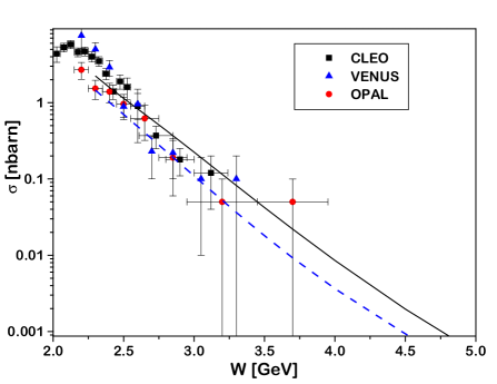
Figure 1: Integrated cross section for $\gamma\gamma\rightarrow p\bar{p}$ ($|\cos(\theta)|<0.6$) versus $W=\sqrt{s}$. The solid line is the complete diquark model prediction, the dashed line is the contribution of only helicity conserving amplitudes, $\bar{\phi}_{1}$ and $\bar{\phi}_{5}$. Data are taken from Refs. CLEO (CLEO), TRISTAN (VENUS), and OPAL (OPAL).

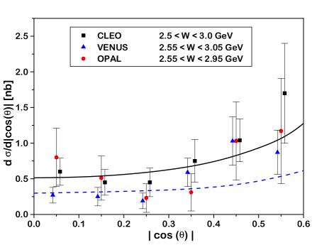
Figure 2: Differential cross section $d\sigma(\gamma\gamma\rightarrow p\bar{p})/d|\cos(\theta)|$) at $W=\sqrt{s}=2.8GeV$. Data are taken from Refs. CLEO (CLEO), TRISTAN (VENUS), and OPAL (OPAL). Solid and dashed lines as in Fig. 1.

In the course of the past decade, large-$|t|$ cross sections for $\gamma\gamma\rightarrow p\bar{p}$ have been measured by various groups CLEO ; TRISTAN ; OPAL . The diquark-model predictions for integrated ($|\cos(\theta)|<0.6$) as well as differential cross sections are seen to lie well within the range of the corresponding data (see Figs. 1 and 2, respectively). The comparison of the solid and the dashed lines shows that the contributions of the mass corrections which enter via the hadronic helicity-flip amplitudes $\bar{\phi}_{2}$, $\bar{\phi}_{4}$, and $\bar{\phi}_{6}$ are of the same order of magnitude as that of the leading-order hadronic helicity conserving amplitudes $\bar{\phi}_{1}$ and $\bar{\phi}_{5}$ . The dashed line corresponds also approximately to the results given in Ref. time , in which quark masses have been neglected completely and the vector-diquark mass has been taken as a fixed parameter. In contrast to our results, the perturbative predictions of the pure quark HSP FMN85 ; FZOZ89 are at least one order of magnitude below the data.

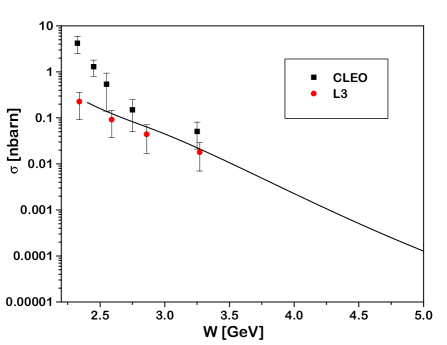
Figure 3: Integrated cross section for $\gamma\gamma\rightarrow\Lambda\bar{\Lambda}$ ($|\cos(\theta)|<0.6$) versus $W=\sqrt{s}$. Data are taken from Refs. CLEO2 (CLEO) and L3 (L3).

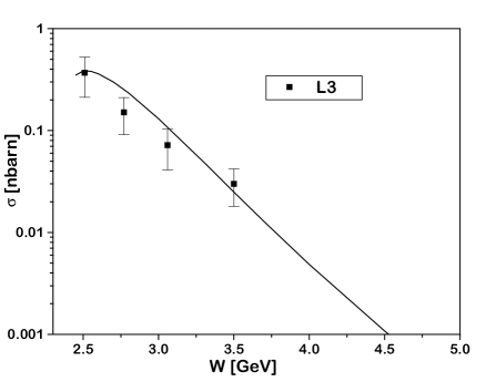
Figure 4: Integrated cross section for $\gamma\gamma\rightarrow\Sigma^{0}\bar{\Sigma}^{0}$ ($|\cos(\theta)|<0.6$) versus $W=\sqrt{s}$. Data are taken from Ref. L3 (L3).

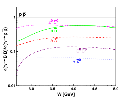
Figure 5: Diquark model predictions for $\gamma\gamma$-annihilation into baryon-antibaryon pairs. Shown are ratios of integrated cross sections $\sigma(\gamma\gamma\rightarrow B\bar{B})/\sigma(\gamma\gamma\rightarrow p\bar{p})$ ($|\cos(\theta)|<0.6$) versus $W=\sqrt{s}$ for neutral baryons.

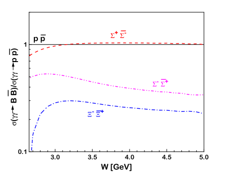
Figure 6: Diquark model predictions for $\gamma\gamma$-annihilation into baryon-antibaryon pairs. Shown are ratios of integrated cross sections $\sigma(\gamma\gamma\rightarrow B\bar{B})/\sigma(\gamma\gamma\rightarrow p\bar{p})$ ($|\cos(\theta)|<0.6$) versus $W=\sqrt{s}$ for charged baryons.

With the SU(3)-symmetric flavor parts of the quark-diquark wave functions given in Tab. 1 and the flavor-dependent distribution amplitude, Eq. (6), we are in the position to treat not only $p\bar{p}$ production, but also the production of other octet-baryon pairs without introducing new parameters. For the $\Lambda$ and $\Sigma^{0}$ channels integrated cross-section data have been published very recently CLEO2 ; L3 . As shown in Fig. 3 our predictions for the $\Lambda$ channel agree favorably with the most recent L3 measurements which are somewhat below the older CLEO data points. Comparable good agreement with the L3 data is also achieved for the $\Sigma^{0}$ channel (cf. Fig. 4). For the other octet-baryon channels we have no experimental information as yet, apart from a statement by the L3 collaboration that the $\Lambda\bar{\Sigma}^{0}+\Sigma^{0}\bar{\Lambda}$ cross section is below their present detection accuracy. In order to have a guideline we have therefore plotted the ratios of integrated $B\bar{B}$ cross sections ($|\cos(\theta)|<0.6$) to the $p\bar{p}$ cross section. These ratios are shown in Fig. 5 and Fig. 6 for neutral and charged baryons, respectively. From these figures one observes that it may be feasible to measure also other hyperon channels like $\Sigma^{+}\bar{\Sigma}^{-}$, $\Sigma^{-}\bar{\Sigma}^{+}$, or $\Xi^{-}\bar{\Xi}^{+}$, since the corresponding cross sections are predicted to be of the same size or even larger than the $\Lambda\bar{\Lambda}$ cross section. Such data could be very useful to determine the amount of SU(3) flavor symmetry breaking in the baryon distribution amplitudes. At asymptotically large momentum transfers $|t|,\;|u|\rightarrow\infty$, where the diquarks dissolve into quarks the three-quark distribution amplitudes of the octet baryons satisfy exact SU(6) spin-flavor symmetry. This leads to relations between the various production cross sections for flavor octet and decuplet baryons farrar . SU(3) flavor symmetry, in particular $U$-spin invariance (which is the symmetry under interchange of $d$ and $s$ quarks) alone, implies already that

$$\sigma(\gamma\gamma\rightarrow p\bar{p})\;\;\;\,\; = \sigma(\gamma\gamma\rightarrow\Sigma^{+}\bar{\Sigma}^{-}),$$ (18)

$$\sigma(\gamma\gamma\rightarrow n\bar{n})\;\;\;\,\; = \sigma(\gamma\gamma\rightarrow\Xi^{0}\bar{\Xi}^{0}),$$ (19)

$$\sigma(\gamma\gamma\rightarrow\Sigma^{-}\!\bar{\Sigma}^{+}) = \sigma(\gamma\gamma\rightarrow\Xi^{-}\bar{\Xi}^{+}).$$ (20)

Two more relations follow from U-spin invariance. These, however, assume only a simple form on the amplitude level:

$$\mathcal{M}^{\Lambda\bar{\Sigma}^{0}} = \sqrt{3}(\mathcal{M}^{\Lambda\bar{\Lambda}}-\mathcal{M}^{n\bar{n}}),$$ (21)

$$\mathcal{M}^{\Sigma^{0}\bar{\Sigma}^{0}} = 3\mathcal{M}^{\Lambda\bar{\Lambda}}-2\mathcal{M}^{n\bar{n}}.$$ (22)

These relations hold for each helicity amplitude. At finite momentum transfers deviations from SU(3)-flavor symmetry have their origin in the different baryon masses and the flavor dependence of the baryon DAs. This is precisely the observation which can be made from Figs. 5 and 6. The larger the mass difference of the produced baryon-antibaryon pair the bigger the violation of SU(3) flavor symmetry. The asymptotic SU(6) spin-flavor symmetry gives rise to additional relations between the amplitudes for octet- and decuplet-baryon production farrar . A systematic breaking of SU(6) spin-flavor symmetry down to SU(3) flavor symmetry is inherent in the diquark model and is caused by the assumption of flavor dependent scalar and vector-diquark masses, different vertex form factors, and different values for $f_{S}$ and $f_{V}$. This kind of symmetry breaking could be investigated by comparing the production of octet and decuplet baryons.

Very recently, the production of baryon pairs has also been investigated within the generalized parton picture in dikrovo . The authors of Ref. dikrovo analyze the handbag contribution to $\gamma\gamma\rightarrow B\bar{B}$ and obtain an expression for the differential $\gamma\gamma\rightarrow B\bar{B}$ cross section which, after some simplifying assumptions, contains only one effective $s$-dependent form factor. After fixing this form factor by means of integrated $p\bar{p}$ cross-section data, the authors employ isospin and $U$-spin invariance to give amplitude ratios $r_{B}=\mathcal{M}^{B\bar{B}}/\mathcal{M}^{p\bar{p}}$ for the other octet baryons $B$. In this way they obtain similar good agreement with the integrated $\Lambda\bar{\Lambda}$ and $\Sigma^{0}\bar{\Sigma}^{0}$ cross section data as we do. In a similar spirit the time-reversed process $p\bar{p}\rightarrow\gamma\gamma$ has been considered in Ref. FRSW02 . In this paper, however, it has been attempted to model directly the time-like double distributions which describe the transition of the $p\bar{p}$ to the $q\bar{q}$ pair. For $s=10$ GeV² the authors predict an integrated cross section ($|\cos(\theta)|<0.7$) of $0.25\times 10^{-9}$ fm². We find a considerably larger cross section, namely $0.14\times 10^{-7}$ fm², which, however, agrees with the estimate of Diehl et al. dikrovo ; kroprivat . Such predictions may be of interest regarding the proposal to build an antiproton storage ring at GSI.

4 The crossed process $\gamma B\rightarrow\gamma B$

Although the focus of the present work is baryon pair production in two-photon collisions, we want to briefly comment on the crossed process, Compton scattering off baryons. Predictions for real and virtual Compton scattering off protons have already been given in Ref. KSG96 for the current parameterization of the diquark model. In the following we will briefly summarize how our improved treatment of constituent masses affects the results for real Compton scattering.

Following the common convention rosti76 we denote the six independent helicity amplitudes for Compton scattering $\mathcal{M}_{\lambda_{2},\,\lambda_{f};\,\lambda_{1},\,\lambda_{i}}$ ($\lambda_{j},\,j=1,2\dots$ helicities of the incoming and outgoing photons, respectively; $\lambda_{i},\,\lambda_{f}\dots$ helicities of the incoming and outgoing baryon, respectively) by

$$\phi_{1} = \mathcal{M}_{1,\,\frac{1}{2};\,1,\,\frac{1}{2}},$$

$$\phi_{2} = \mathcal{M}_{-1,\,-\frac{1}{2};\,1,\,\frac{1}{2}},$$

$$\phi_{3} = \mathcal{M}_{-1,\,\frac{1}{2};\,1,\,\frac{1}{2}},$$

$$\phi_{4} = \mathcal{M}_{1,\,-\frac{1}{2};\,1,\,\frac{1}{2}},$$

$$\phi_{5} = \mathcal{M}_{1,\,-\frac{1}{2};\,1,\,-\frac{1}{2}},$$

$$\phi_{6} = \mathcal{M}_{-1,\,\frac{1}{2};\,1,\,-\frac{1}{2}}.$$ (23)

These amplitudes are related to those for the crossed reaction $\gamma\gamma\rightarrow B\bar{B}$ (see Eq. (2)) via the crossing relations:

$$\overline{\phi}_{1} = \phi_{1}+2m_{B}\sqrt{\frac{\hat{u}}{\hat{s}\,\hat{t}}}\,\phi_{4},$$

$$\overline{\phi}_{2} = \phi_{2}-2m_{B}\sqrt{\frac{\hat{u}}{\hat{s}\,\hat{t}}}\,\phi_{3},$$

$$\overline{\phi}_{3} = \phi_{3}+m_{B}\sqrt{\frac{\hat{u}}{\hat{s}\,\hat{t}}}\,\left(\phi_{2}-\phi_{6}\right),$$

$$\overline{\phi}_{4} = \phi_{4}-m_{B}\sqrt{\frac{\hat{u}}{\hat{s}\,\hat{t}}}\,\left(\phi_{1}+\phi_{5}\right),$$ (24)

$$\overline{\phi}_{5} = -\phi_{5}-2m_{B}\sqrt{\frac{\hat{u}}{\hat{s}\,\hat{t}}}\,\phi_{4},$$

$$\overline{\phi}_{6} = -\phi_{6}-2m_{B}\sqrt{\frac{\hat{u}}{\hat{s}\,\hat{t}}}\,\phi_{3},$$

where $\overline{\phi}_{i}=\overline{\phi}_{i}\left(\hat{t},\hat{u}\right)$ and $\phi_{i}=\phi_{i}\left(\hat{s},\hat{u}\right)$. That is, we exchange $\hat{s}\leftrightarrow\hat{t}$ (if $\hat{s}$ occurs as argument of a square root it has to be replaced by $|\hat{t}|$). The above relations are expanded up to first order in the baryon mass.

We have used these crossing relations to check our analytical expressions for the elementary $\gamma\gamma\rightarrow qD\bar{q}\bar{D}$ and $\gamma qD\rightarrow\gamma qD$ amplitudes which have been calculated separately. Since the explicit calculations agree with the crossing relations (4), we refrain from listing the various amplitudes contributing to $\gamma B\rightarrow\gamma B$. They can be read off from the expressions for $\gamma\gamma\rightarrow B\bar{B}$ listed in Tables 3 and 4, with the appropriate replacements $\hat{s}\leftrightarrow\hat{t}$. A further check of our analytical expressions is the comparison in the massless limit with the earlier results of Refs. Compton ; KSG96 .

The numerical integrations in the convolution integral (1) deserve special care, since the gluon-propagators appearing in the 4-point functions,

$$g_{1}^{-2} = (x_{2}y_{1}\,\hat{u}+x_{1}y_{2}\hat{s})^{-1},$$

$$g_{2}^{-2} = (x_{2}y_{1}\,\hat{s}+x_{1}y_{2}\hat{u})^{-1},$$ (25)

can go on-shell. The resulting propagator poles have to be treated with a principal value prescription,

$$\frac{1}{g^{2}+i\varepsilon}=\wp\left(\frac{1}{g^{2}}\right)-i\pi\delta(g^{2}).$$ (26)

Here we do not go into the technical details of implementing this prescription numerically, but rather refer the reader to CW for further explanation. We only want to emphasize, that our numerical results are absolutely stable for both real and imaginary parts.

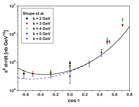
Figure 7: Scaled differential cross section $s^{6}\ d\sigma(\gamma p\rightarrow\gamma p)/dt$. Diquark-model predictions are given for the photon lab energy $k=4$ GeV ($W=\sqrt{s}=2.9$ GeV) with all (solid line) and only hadronic helicity conserving amplitudes (dashed line) taken into account. Data for various photon lab energies are taken from Ref. shu79

As can be seen from Fig. 7 the predictions of the diquark model agree nicely with the few available differential cross-section data at intermediately large momentum transfers. According to a recent study brooksdix it seems to be unlikely, on the other hand, that the pure quark HSP is able to account for these data. Good results, however, are also obtained within the generalized parton picture with its dominant contribution being given by the handbag diagram rad98 ; kroll2 . In this case only one parton undergoes a hard scattering. The (soft) emission and reabsorption of the parton by the hadron is described by generalized parton distributions which may be modelled by the overlaps of light-cone wave functions, since the change of the parton momentum is space-like. It is not surprising that our diquark model which is based on the hard-scattering picture yields results similar to the soft overlap mechanism. It indicates that part of the multidimensional overlap integral is absorbed into diquark form factors which, in our model, are parameterized phenomenologically over the whole momentum-transfer range.

There are, nevertheless, qualitative differences between the diquark model and the overlap mechanism which appear, in particular, in polarization observables. As a representative example let us, e.g., mention the initial state helicity correlation $A_{LL}$. Whereas the soft overlap yields positive values for this spin observable kroll2 , we obtain a negative result within the diquark model. This difference can be understood easily. The comparison of the solid and the dashed lines in Fig. 7 reveals that the (leading order) hadronic helicity conserving amplitudes $\phi_{1}$ and $\phi_{5}$ are dominant. Mass corrections, which enter via the hadron-helicity-flip amplitudes $\phi_{2}$, $\phi_{4}$, and $\phi_{6}$, only start to play a role in the backward region. Thus $A_{LL}$ is roughly given by the difference $(|\phi_{1}|^{2}-|\phi_{5}^{2}|)$. Considering the analytical expressions for these amplitudes (cf. Tabs. 3 and 4 with $\hat{s}\leftrightarrow\hat{t}$ interchanged), specifically the 3-point contributions, which are actually the most important ones, we see that $(|\phi_{1}|^{2}-|\phi_{5}|^{2})\propto(1/(x_{2}^{2}y_{2}^{2})-1/(x_{1}^{2}y_{1}^{2}))(\hat{s}^{2}-\hat{u}^{2})/(\hat{t}^{2}\hat{s}|\hat{u}|)$. For our choice of quark-diquark distribution amplitudes the average values of the momentum fractions are $<x_{1}>=<y_{1}>=1-<x_{2}>=1-<x_{2}>\approx 1/3$ so that one can already conclude that $A_{LL}$ should be negative. This is indeed the result of our numerical calculations. These considerations illustrate also why the soft overlap mechanism provides a positive $A_{LL}$. Within such an approach the active quark carries nearly all of the baryon momentum ($x_{1},y_{1}\approx 1$) and hence $(1/(x_{2}^{2}y_{2}^{2})-1/(x_{1}^{2}y_{1}^{2}))$ becomes positive. By similar qualitative arguments we expect the spin-transfer parameter $D_{LL}$ to be close to $1$ and the photon asymmetry $\Sigma$ to be close to $0$. Our numerical calculations confirm these estimates. They show in addition that polarization observables are, unlike spin averaged quantities, very sensitive to the choice of the quark-diquark distribution amplitudes. Experimental data for such observables could thus be helpful to determine the (phenomenological) quark-diquark distribution amplitudes unambiguously.

5 Final remarks

In this work we have investigated exclusive two-photon reactions at moderately large momentum transfer within a quark-diquark model. This approach is a modification of the pure quark hard-scattering picture where baryons are treated as systems of quarks and diquarks. The work continues and extends the systematic study of photon-induced exclusive hadronic reactions gamgampp ; Compton ; fixed ; time ; KSG96 ; KSPS97 ; fizb ; CW ; mass performed within the same approach. The introduction of diquarks allows us to extend the range of validity of the pure quark HSP down to the kinematic region of a few GeV of momentum transfer, as this modelling accounts for nonperturbative effects present in this region. This is also the kinematic range which is accessible with present-day experimental facilities.

We have extended previous calculations of the two-photon reactions $\gamma\gamma\rightarrow B\bar{B}$ and $\gamma B\rightarrow\gamma B$ gamgampp ; Compton ; time . Refs. Compton and time have only dealt with the proton channel, Ref. gamgampp has investigated other baryon channels as well, but under the simplifying assumption that vector diquarks can be neglected compared to scalar ones. In Refs. gamgampp ; Compton ; time mass effects have been treated in a simplified way, so that the crossing relations between the $\gamma\gamma\rightarrow B\bar{B}$ and the $\gamma B\rightarrow\gamma B$ channels were only exactly fulfilled for the dominant helicity-nonflip amplitudes. In this work we have studied all octet baryon channels with an improved treatment of mass effects by systematically expanding in the small parameter (mass/photon energy). We have performed our calculations within the complete diquark model, that is, with scalar and vector diquarks. For the two-photon annihilation mass corrections are found to be sizable. Their inclusion considerably improves the agreement of the diquark model predictions with the recent LEP data for two-photon annihilation into $\Lambda\bar{\Lambda}$ and $\Sigma^{0}\bar{\Sigma}^{0}$. On the other hand, mass corrections seem to be of minor importance in Compton scattering. It would certainly be desirable to obtain experimental baryon pair-production data for hyperons different from $\Lambda$ or $\Sigma^{0}$. For $\Sigma^{+}$, $\Sigma^{-}$, and $\Xi^{-}$ we find cross sections of comparable size so that one may hope that corresponding measurements could be feasible. Such data could provide information on the flavor dependence of baryon distribution amplitudes, and they could help to decide whether the particular scheme of $SU(6)$ spin-flavor-symmetry breaking inherent to the diquark model is appropriate.

Finally we want to emphasize that to the best of our knowledge the diquark model is, aside from the generalized parton picture, the only constituent-scattering model which is able to account for the $\gamma\gamma\rightarrow p\bar{p}$, $\gamma\gamma\rightarrow\Lambda\bar{\Lambda}$, $\gamma\gamma\rightarrow\Sigma\bar{\Sigma}$, and $\gamma p\rightarrow\gamma p$ data at intermediately large momentum transfer. It is even more remarkable that this is achieved with the set of model parameters that provides also a reasonable description of other exclusive quantities, like electromagnetic nucleon factors fixed ; time or photoproduction cross sections KSPS97 ; CW . Therefore further applications of this effective approach and studies of its underlying mechanisms are certainly worthwhile.

Appendix A Feynman Rules

A.1 Three-point vertices

• SgS-vertex:

  $$\mbox{\small i}\mbox{g}_{\mbox{\scriptsize s}}T^{a}_{ij}(p_{1}+p_{2})_{\mu}$$ (27)

• S$\gamma$S-vertex:

  $$-\mbox{\small i}\mbox{e}_{0}\mbox{e}_{S}(p_{1}+p_{2})_{\mu}$$ (28)

• VgV-vertex:

  $$-\mbox{\small i}\mbox{g}_{\mbox{\scriptsize s}}T^{a}_{ij} \Big{\{} \mbox{g}_{\alpha\beta}(p_{1}+p_{2})_{\mu}$$ (29)

  $$- \mbox{g}_{\mu\alpha}\left[(1+\kappa_{V})p_{1}-\kappa_{V}p_{2}\right]_{\beta}$$

  $$- \mbox{g}_{\mu\beta}\left[(1+\kappa_{V})p_{2}-\kappa_{V}p_{1}\right]_{\alpha}\Big{\}}$$

• V$\gamma$V-vertex:

  $$\mbox{\small i}\mbox{e}_{0}\mbox{e}_{V} \Big{\{} \mbox{g}_{\alpha\beta}(p_{1}+p_{2})_{\mu}$$ (30)

  $$- \mbox{g}_{\mu\alpha}\left[(1+\kappa_{V})p_{1}-\kappa_{V}p_{2}\right]_{\beta}$$

  $$- \mbox{g}_{\mu\beta}\left[(1+\kappa_{V})p_{2}-\kappa_{V}p_{1}\right]_{\alpha}\Big{\}}$$

A.2 Four-point vertices

• $\gamma$SgS-vertex:

  $$-2\mbox{\small i}\mbox{e}_{0}\mbox{e}_{S}\mbox{g}_{\mbox{\scriptsize s}}T^{a}_{ij}\mbox{g}_{\mu\nu}$$ (31)

• $\gamma$S$\gamma$S-vertex:

  $$2\mbox{\small i}\mbox{e}^{2}_{0}\mbox{e}^{2}_{S}\mbox{g}_{\mu\nu}$$ (32)

• gSgS-vertex:

  $$\mbox{\small i}\mbox{g}^{2}_{\mbox{\scriptsize s}}\left\{T^{a},T^{b}\right\}_{ij}\mbox{g}_{\mu\nu}$$ (33)

• $\gamma$VgV-vertex:

  $$\mbox{\small i}\mbox{e}_{0}\mbox{e}_{V}\mbox{g}_{\mbox{\scriptsize s}}T^{a}_{ij}(2\mbox{g}_{\mu\nu}\mbox{g}_{\alpha\beta}-\mbox{g}_{\mu\beta}\mbox{g}_{\alpha\nu}-\mbox{g}_{\mu\alpha}\mbox{g}_{\beta\nu})$$ (34)

• $\gamma$V$\gamma$V-vertex:

  $$-\mbox{\small i}\mbox{e}_{0}^{2}\mbox{e}_{V}^{2}(2\mbox{g}_{\mu\nu}\mbox{g}_{\alpha\beta}-\mbox{g}_{\mu\beta}\mbox{g}_{\alpha\nu}-\mbox{g}_{\mu\alpha}\mbox{g}_{\beta\nu})$$ (35)

• gVgV-vertex:

  $$-\mbox{\small i}\mbox{g}^{2}_{\mbox{\scriptsize s}} \Big{\{} \left\{T^{a},T^{b}\right\}_{ij}\mbox{g}_{\mu\nu}\mbox{g}_{\alpha\beta}$$

  $$- \left[(1+\kappa_{V})(T^{a}T^{b})_{ij}-\kappa_{V}(T^{b}T^{a})_{ij}\right]\mbox{g}_{\mu\beta}\mbox{g}_{\alpha\nu}$$

  $$- \left[(1+\kappa_{V})(T^{b}T^{a})_{ij}-\kappa_{V}(T^{a}T^{b})_{ij}\right]\mbox{g}_{\mu\alpha}\mbox{g}_{\beta\nu}\Big{\}}$$

Here $e_{\mbox{\scriptsize q}},e_{S},e_{V}$ are the charges of quarks, scalar and vector diquarks respectively, $e_{0}=\sqrt{4\pi\alpha}$ denotes the elementary charge with the fine structure constant $\alpha\approx 1/137$, $g_{S}=\sqrt{4\pi\alpha_{s}}$ is the strong coupling constant of QCD, and $T^{a}$ represent the Gell-Mann color matrices.

References

• (1) S. J. Brodsky, G. P. Lepage, Exclusive Processes in Quantum Chromodynamics, in Perturbative Quantum Chromodynamics (World Scientific, Singapore 1989) p. 93.
• (2) B. Pire, Exclusive reactions in QCD, in Les Houches 1996, Trends in nuclear physics, 100 years later (1996) p. 567, [nucl-th/9612009].
• (3) N. G. Stefanis, Eur. Phys. J. direct C 7, (1999) 1, [hep-ph/9911375].
• (4) N. Isgur, C. Llewellyn Smith, Phys. Lett. B 217, (1989) 535.
A. P. Bakulev, A. V. Radyushkin, Phys. Lett. B 271, (1991) 223.
P. Kroll, hep-ph/9511452.
• (5) M. Anselmino, P. Kroll, B. Pire, Z. Phys. C 36, (1987) 89.
• (6) M. Anselmino, F. Caruso, P. Kroll, W. Schweiger, Int. J. Mod. Phys. A 4, (1989) 5213.
• (7) P. Kroll, M. Schürmann, W. Schweiger, Int. J. Mod. Phys. A 6, (1991) 4107.
• (8) R. Jakob, P. Kroll, M. Schürmann, W. Schweiger, Z. Phys. A 347, (1993) 109, [hep-ph/9310227].
• (9) P. Kroll, Th. Pilsner, M. Schürmann, W. Schweiger, Phys. Lett. B 316, (1993) 546, [hep-ph/9305251].
• (10) R. Jakob, Phys. Rev. D 50, (1994) 5647, [hep-ph/9406250].
• (11) P. Kroll, M. Schürmann, P. A. M. Guichon, Nucl. Phys. A 598, (1996) 435, [hep-ph/9507298].
• (12) P. Kroll, M. Schürmann, K. Passek, W. Schweiger, Phys. Rev. D 55, (1997) 4315, [hep-ph/9604353].
• (13) C. F. Berger, B. Lechner, W. Schweiger, Fizika B 8, (1999) 371, [hep-ph/9901338].
• (14) C. F. Berger, W. Schweiger, Phys. Rev. D 61, (2000) 114026, [hep-ph/9910509].
• (15) C. F. Berger, B. Jäger , W. Schweiger, Nucl. Phys. A 689, (2001) 390, [hep-ph/0009295].
B. Jäger, W. Schweiger, Nucl. Phys. A 711, (2002) 203, [hep-ph/0206189].
• (16) G. P. Lepage, S. J. Brodsky, Phys. Rev. D 22, (1980) 2157.
• (17) A. V. Efremov, A. V. Radyushkin, Phys. Lett. B 94, (1980) 245.
• (18) M. Anselmino et al., Rev. Mod. Phys. 65, (1993) 1199.
• (19) B. Lechner, Diploma thesis, University Graz (1997), unpublished.
• (20) M. Schwärz, Diploma thesis, University Graz (2001), unpublished.
M. Schwärz, W. Schweiger, AIP Conf. Proc. 603, (2001) 381, [hep-ph/0109143].
• (21) H. Rollnik, P. Stichel, Springer Tracts in Modern Physics 79, (1976) 1.
• (22) T. Huang, Nucl. Phys. Proc. Suppl. B 7, (1989) 320.
• (23) J. J. Aubert et al., Phys. Lett. B 95, (1980) 306.
• (24) M. G. Sotiropoulos, G. Sterman, Nucl. Phys. B 425, (1994) 489, [hep-ph/9401237].
• (25) A. H. Mueller, Phys. Rept. 73, (1981) 237.
J. Botts, G. Sterman, Nucl. Phys. B 325, (1989) 62.
H.-n. Li, G. Sterman, Nucl.Phys. B 381, (1992) 129.
H.-n. Li, Phys. Rev. D 48, (1993) 4243.
• (26) M. Anselmino, F. Caruso, F. Murgia, Phys. Rev. D 42, (1990) 3218.
• (27) CLEO Collaboration (M. Artuso et al.), Phys. Rev. D 50, (1994) 5484.
• (28) VENUS Collaboration (H. Hamasaki et al.), Phys. Lett. B 407, (1997) 185.
• (29) OPAL Collaboration (G. Abbiendi et al.), hep-ex/0209052.
• (30) G. R. Farrar, E. Maina, F. Neri, Nucl. Phys. B 259, (1985) 702; ibid. B 263 (1986) 746 (E).
• (31) G. R. Farrar, H. Zhang, A. A. Ogloblin, I. R. Zhitnitsky, Nucl. Phys. B 311, (1989) 585.
• (32) CLEO Collaboration (S. Anderson et al.), Phys. Rev. D 56, (1997) 2485, [hep-ex/9701013].
• (33) L3 Collaboration (P. Achard et al.), Phys. Lett. B 536, (2002) 24, [hep-ex/0204025].
• (34) G. R. Farrar, Phys. Rev. Lett. 53, (1984) 28.
• (35) M. Diehl, P. Kroll, C. Vogt, hep-ph/0206288.
• (36) A. Freund, A. V. Radyushkin, A. Schäfer, C. Weiss, hep-ph/0208061.
• (37) P. Kroll, private communication.
• (38) M. A. Shupe et al., Phys. Rev. D 19, (1979) 1921.
• (39) T. C. Brooks, L. J. Dixon, Phys. Rev. D 62, (2000) 114021, [hep-ph/0004143].
• (40) A. V. Radyushkin, Phys. Rev. D 58, (1998) 114008, [hep-ph/9803316].
• (41) M. Diehl, T. Feldmann, R. Jakob, P. Kroll, Eur. Phys. J. C 8, (1999) 409, [hep-ph/9811253]; Phys. Lett. B 460, (1999) 204, [hep-ph/9903268].
H. W. Huang, P. Kroll, T. Morii, Eur. Phys. J. C 23, (2002) 301, [hep-ph/0110208].