FTUAM-02/32; IFT-UAM/CSIC-02-55

hep-ph/0212064

Towards a theory of quark masses, mixings and CP-violation
D. Cremades, L.E. Ibáñez and F. Marchesano
Departamento de Física Teórica C-XI and Instituto de Física Teórica C-XVI,
Universidad Autónoma de Madrid, Cantoblanco, 28049 Madrid, Spain.
Abstract

We discuss the structure of Yukawa couplings in D-brane models in which the SM fermion spectrum appears at the intersections of D-branes wrapping a compact space. In simple toroidal realistic examples one can explicitly compute the Yukawa couplings as a function of the geometrical data summing over world-sheet instanton contributions. A particular simple model with a $N=1$ SUSY spectrum and three quark-lepton generations is studied in some detail. Remarkably, one can reproduce the observed spectrum of quark masses and mixings for particular choices of the compact radii and brane locations. In order to reproduce the smallness of up- and down-quark masses branes should be located in simple geometric configurations leading to some accidental global symmetries. We also find that the brane configurations able to reproduce the observed data may be considered as a deformation (by brane translation) of a configuration with Pati-Salam gauge symmetry. The origin of CP-violation in this formalism is quite elegant. It appears as a consequence of the generic presence of $U(1)$ Wilson line backgrounds in the compact dimensions. One can reproduce the observed results for the CP-violation Jarlskog invariant J as long as the compact radii are of order of the string scale.

DISCLAIMER: This paper is going to be substantially revised. Althought the physics and general concepts are still valid, the Yukawa couplings of the particular model presented in this paper have a simpler form than discussed here, as we recently pointed out in hep-th/0302105. A properly revised version will be eventually sent as the paper is appropriately corrected.

1 Introduction

One of the most outstanding puzzles of the standard model (SM) is the structure of fermion masses and mixing angles. The masses of quark and leptons are clearly not random, showing a hierarchical structure (see table 1) with masses differing by several orders of magnitude.

U-quarks	u	c	t
	0.9-2.9 MeV	530-680  MeV	168-180 GeV
D-quarks	d	s	b
	1.8-5.3 MeV	35-100 MeV	2.8-3.0  GeV
Leptons	e	$\mu$	$\tau$
	0.51  MeV	105.6  MeV	1.777  GeV

Table 1: Masses of quarks and leptons at the $M_{Z}$ scale taken from the first paper in ref. [1].

Something similar happens with the electroweak CKM mixing matrix which numerically is given (for the moduli of the entries) by [2]

$$\begin{array}[]{cc}&\\ \left|V_{CKM}\right|\ =&\left(\begin{array}[]{ccc}0.9741-0.9756&0.219-0.226&0.0025-0.0048\\ 0.219-0.226&0.9732-0.9748&0.038-0.044\\ 0.004-0.014&0.037-0.044&0.9990-0.9993\end{array}\right)\ .\end{array}$$ (1.1)

at the 90% confidence level. This is close to a unit matrix with small off-diagonal mixing except for the Cabibbo (12) entry which is somewhat larger. Again there is a hierarchical structure with the third generation mixing mostly with the second generation rather than the first. The violation of CP is given in the “standard” parametrization [2] by the phase $\delta_{13}=59^{0}\pm 13^{0}$, which may be considered rather large. A convention independent measure of CP-violation [3] is given by the Jarlskog invariant J which experimentally is [2] $J=(3.0\pm 0.3)\times 10^{-5}$.

The understanding of the structure of fermion masses and mixings has been the subject of an enormous amount of effort. A phenomenological attitude widely followed is to consider fermion mass “textures” or definite ansatze for the form of the mass matrices (see, e.g.,[1] and references therein). In the presence of “texture zeros” one can obtain relationships between the mixing angles and quark masses like the approximate numerical equality [4] $sin\ \theta_{12}=\sqrt{m_{d}/m_{s}}$. Attempts to understand the presence of such “textures” have been made in different flavour models, one of the simplest being based in Abelian flavour symmetries [5, 6]. Grand unified theories combined with textures have also been systematically explored in order to understand the fermion spectrum (see, e.g., [7] and references therein). In spite of the fact that these and other approaches can give a semiquantitative understanding of the fermion spectrum, we are still lacking a full explanation of the masses and mixings in terms of a more fundamental theory. An obvious candidate for such a more fundamental theory is string theory. In fact the structure of fermion masses has been studied in a number of semirealistic heterotic string models. Although one can reproduce interesting features of the observed spectrum, one limitation of this approach is that usually the obtained models have (at least before field theory flat directions are taken) additional fermions, gauge and Higgs bosons which make the analysis complicated.

In spite of that, string theory has a priori a theoretical advantage for addressing this puzzle: the Yukawa couplings may be computable as functions of the geometrical moduli in particular models. That is the case, for example of Abelian ${\bf Z}_{N}$ orbifold compactifications in which one can use conformal field theory (CFT) techniques to compute them [8] . In fact, string theory contains built-in a possible mechanism in order to obtain hierarchical Yukawa couplings [9]. In such orbifold models some matter fields are localized in extra dimensions in the different fixed points of the orbifold. Thus one can imagine an scenario in which the Higgs field lives in one of the fixed points and the different right- and left-handed fermions live in different distant fixed points. Yukawa couplings between quarks which are distant from the Higgs are mediated by world-sheet instanton effects and are hence exponentially suppressed by the (distance)² between the different fixed points [9] . The corresponding Yukawa couplings may be explicitly computed in terms of the geometry of the given orbifold. Although from the theoretical point of view this is fine, phenomenologically the problem arises because in such ${\bf Z}_{N}$ heterotic orbifolds searches for models with just three generations and a minimal Higgs sector have been unsuccessful.

With the advent of D-branes in Type II and type I string theory, the phenomenological possibilities of string theory have widened in several respects (see ref. [10, 11, 12, 13, 14, 15, 16, 17, 18, 19, 20, 21, 22, 23, 24, 25, 26, 27] for the construction of explicit D-brane semirealistic string configurations). In particular, there is now the possibility of following a “bottom-up” approach [10, 26] to the construction of semirealistic three-generation models, i.e., one can consider local D-brane configurations giving rise to the gauge group of the SM and three quark-lepton generations and then embed such a local configuration in some general compactification. Many properties of the models depend only on the local brane configuration, rather than on the details of the particular compact (e.g., Calabi-Yau) space.

In the present paper we address the computation of Yukawa couplings in D-brane models. We concentrate on a recently constructed class of D-brane models [12, 13, 14, 15, 16, 17, 18, 19, 20, 21, 22, 23, 24, 25, 26, 27] in which the SM chiral spectrum is obtained at intersecting branes (for short reviews see, e.g., [28, 29]). Nevertheless, we believe the approach is much more general since Yukawa couplings in other type of D-brane models (like those based on D-branes at orbifold singularities or those involving D-branes with magnetic fluxes [30]) are related by T-duality and/or mirror symmetry with intersecting brane configurations [31, 26].

One of the advantages of the present approach is that, unlike what happened in heterotic constructions, it is relatively easy to find D-brane string configurations yielding (at least for the chiral spectrum) just the particle content of the SM (or the MSSM) already at the string level, i.e., without any further effective field theory elaboration [16, 20]. The simplest such models involve orientifold compactifications of Type IIA string theory on a 6-torus $T^{2}\times T^{2}\times T^{2}$. The Yukawa couplings in these schemes correspond to string correlators involving the Higgs scalar, one right-handed and one left-handed fermion [14]. The worldsheets corresponding to those correlators have then a triangular shape with the fields at the intersections and the sides embedded on the three different intersecting stacks of branes (see figure 1). The leading contribution to the Yukawa couplings is then given by worldsheet instanton contributions proportional to $exp(-S_{cl})=exp(-A_{abc})$, where $A_{abc}$ is the area of the triangles [14]. In this paper we will focus mainly on the phenomenological applications of such computations and leave the derivation of general expressions for the Yukawa couplings for arbitrary toroidal Dp-brane configurations for a separate paper [32].

Figure 1: Yukawa coupling between two quarks of opposite chirality and a Higgs boson.

In order to show the possibilities of the approach, we compute the Yukawa couplings for a new simple model yielding the chiral spectrum of the MSSM at the intersection of D6-branes wrapping a 6-torus . We provide explicit simple formulae for the relevant Yukawa couplings in terms of world-sheet instanton sums over the cycles of the 6-torus. In some particular geometrical configurations the Yukawa couplings may be written as products of Jacobi $\theta$-functions with characteristics. One of the nicest features we find is a natural origin for the complex phases necessary for CP-violation. In the present approach they correspond to the generic presence of non-trivial Wilson line backgrounds associated to the Abelian gauge symmetries of the theory.

We have performed a search for particular D-brane geometries in this model capable of describing the observed quark masses, mixings and CP-violation parameters. We have found that for certain torus radii and D6-brane locations one can reproduce the observed quark masses and mixing angles. On the other hand we also find the interesting result that, in order to reproduce the observed size for CP-violation, the compact radii of two of the tori have to be of order the string scale, otherwise the phases get exponentially suppressed as the radii increase. The D6-brane locations reproducing the observed data are close to positions in the tori with certain symmetry properties. At those symmetric positions pairs of triangles corresponding to different quark generations become equal, signalling some accidental global symmetries.

Finally we find that the observed spectrum of fermion masses and mixings is consistent with the existence of an underlying (broken) Pati-Salam symmetry [33]. More precisely, the brane configurations able to reproduce the observed data may be considered as a deformation (by brane translation) of a configuration leading to a Pati-Salam symmetry.

The structure of the rest of the paper is as follows. In the next chapter we give a brief introduction to intersecting brane models and present the specific model to be analyzed numerically afterwards. In chapter three we present the form of the expressions for the Yukawa couplings and discuss the origin of symmetries and CP-violation. In chapter four we perform a numerical analysis and show how all quark masses, mixings and CP-violation parameters may be reproduced with the given Yukawa coupling formulae. We also extend the discussion to charged lepton and (Dirac) neutrino masses, mixings and CP-violation. We leave chapter five for some final comments and conclusions.

2 Intersecting brane standard models

A particular class of models with intersecting D-branes has received recently considerable attention, [12, 13, 15, 16]. These are models in which one has four stacks of intersecting D-branes in an orientifold of Type IIA string theory. The four stacks come under the names of baryonic, left, right and leptonic and each stack gives rise to the gauge groups $SU(3)$, $SU(2)_{L}$, $U(1)_{R}$ and $U(1)_{lepton}$ respectively (with possibly additional $U(1)$’s). Open strings at the intersections give rise to chiral fermions with the quantum numbers of SM quarks and leptons. In one of the simplest class of models the Type IIA string is compactified on a 6-torus $T^{2}\times T^{2}\times T^{2}$ and D6-branes wrap some cycles of the tori. Specifically, the 7-dimensional worldvolume of D6-branes contains Minkowski space and the three remaining dimensions of the D6-branes wrap one-cycles at each of the three 2-tori of the $T^{6}$ (see figure 2). Let us denote by $(n_{a}^{i},m_{a}^{i})$, $i$ = 1,2,3 the wrapping numbers of each brane $D6_{a}$, $n_{a}^{i}$ ($m_{a}^{i}$) being the number of times the brane stack $a$ is wrapping around the $x$($y$)-coordinate of the $i^{th}$ torus. One can check that the number of times two branes $D6_{a}$ and $D6_{b}$ intersect in $T^{6}$ is given by the intersection number [12]:

$$I_{ab}\ =\ (n_{a}^{1}m_{b}^{1}-m_{a}^{1}n_{b}^{1})(n_{a}^{2}m_{b}^{2}-m_{a}^{2}n_{b}^{2})(n_{a}^{3}m_{b}^{3}-m_{a}^{3}n_{b}^{3})$$ (2.1)

Figure 2: Intersecting brane world setup. Consider two D6-branes filling four non-compact dimensions, to be identified with $M_{4}$, and wrapping three 1-cycles of $T^{2}\times T^{2}\times T^{2}$. In this example the wrapping numbers are $(2,1)(1,0)(1,1)$ (solid line) and $(0,1)(1,2)(0,1)$ (dashed line). The total intersection number is $2\times 2\times 1=4$.

Open strings stretching around the intersections give rise to chiral fermions in the bifundamental representation $(N_{a},{\overline{N}}_{b})$ under the gauge group of the two branes $U(N_{a})\times U(N_{b})$. Thus, these configurations yield $I_{ab}$ copies of the same bifundamental representation, providing a natural source for the observed generation replication. In fact, because of technical reasons one performs an “orientifold” twist [34] of this theory by the product $\Omega\times{\cal R}$, where $\Omega$ is the worldsheet parity operator and ${\cal R}$ is the reflection with respect to the horizontal axis of the three tori. Now, for consistency of the construction, one has to include in the D6-brane configuration mirror branes $D6_{a*}$ for each original $D6_{a}$-brane, wrapping geometrical loci that are mirror with respect to the reflection operation ${\cal R}$. In particular, this implies that their wrapping numbers will be $(n_{a}^{i},-m_{a}^{i})$, rather than $(n_{a}^{i},m_{a}^{i})$. Being part of the same dynamical object, both $D6_{a}$ and $D6_{a*}$ branes correspond to the same gauge group, generically $U(N_{a})$. The chiral fermions arising from the intersection $ab$*, though, will transform in the bifundamental representation $(N_{a},N_{b})$, rather than $(N_{a},{\overline{N}}_{b})$. Finally, when branes $a$ and $a$* coincide, the gauge group may be enhanced from $U(N_{a})$ to $SO(2N_{a})$ or $USp(2N_{a})$.

Let us now show a particular D-brane configuration giving rise to three quark-lepton generations. This model has not been studied previously and we chose it here because of its simplicity and because it naturally contains a minimal Higgs sector which makes very simple the study of Yukawa couplings. Consider the stacks of D6-branes with the wrapping numbers of table 2.

$N_{i}$	$(n_{i}^{1},m_{i}^{1})$	$(n_{i}^{2},m_{i}^{2})$	$(n_{i}^{3},m_{i}^{3})$
$N_{a}=3$	$(1,0)$	$(1/\rho,3\rho)$	$(1/\rho,-3\rho)$
$N_{b}=1$	$(0,1)$	$(1,0)$	$(0,-1)$
$N_{c}=1$	$(0,1)$	$(0,-1)$	$(1,0)$
$N_{d}=1$	$(1,0)$	$(1/\rho,3\rho)$	$(1/\rho,-3\rho)$

Table 2: D6-brane wrapping numbers giving rise to the chiral spectrum of the MSSM. The discrete parameter $\rho=1,1/3$ describes two different sets of wrapping numbers yielding the same intersection numbers (2.2). The addition of the mirror branes is understood.

Generically, the gauge group of this configuration is $U(3)\times U(1)^{3}$. However, one can check that the symmetry is enhanced to $U(3)_{a}\times SU(2)_{b}\times U(1)_{c}\times U(1)_{d}$ if the brane $b$ is located on top of its orientifold mirror $b$*. Computing the intersection numbers as above one gets the result

$$\begin{array}[]{lcl}I_{ab}\ =\ 3,&&I_{ab*}\ =\ 3,\\ I_{ac}\ =\ -3,&&I_{ac*}\ =\ -3,\\ I_{db}\ =\ 3,&&I_{db*}\ =\ 3,\\ I_{dc}\ =\ -3,&&I_{dc*}\ =\ 3,\\ I_{bc}\ =\ -1,&&I_{bc*}\ =\ 1,\end{array}$$ (2.2)

which corresponds to the chiral fermion spectrum of the SM (plus right-handed neutrinos, see table 3). In addition there is a minimal set of Higgs multiplets if one locates the brane $b$ on top of the brane $c$ along the first torus (otherwise the branes do not intersect and the state is massive). In other words, there is a minimal Higgs sector with a $\mu$-parameter whose real part is given by the distance between branes $b$ and $c$ along the first torus (see figure 4 below) and its imaginary part is proportional to the relative phase of their Wilson lines in the same torus.

Intersection	Matter fields		$Q_{a}$	$Q_{c}$	$Q_{d}$	Y
(ab),(ab*)	$Q_{L}$	$3(3,2)$	1	0	0	1/6
(ac)	$U_{R}$	$3({\bar{3}},1)$	-1	1	0	-2/3
(ac*)	$D_{R}$	$3({\bar{3}},1)$	-1	-1	0	1/3
(db),(db*)	$L$	$3(1,2)$	0	0	1	-1/2
(dc)	$N_{R}$	$3(1,1)$	0	1	-1	0
(dc*)	$E_{R}$	$3(1,1)$	0	-1	-1	1
(cb),(cb*)	$H_{u,d}$	$(1,2)$	0	$\pm 1$	0	$\mp 1/2$

Table 3: Standard model spectrum and $U(1)$ charges. The hypercharge generator is defined as $Q_{Y}=\frac{1}{6}Q_{a}-\frac{1}{2}Q_{c}-\frac{1}{2}Q_{d}$.

If the ratios of radii in the second and third tori are equal ($R_{2}^{(2)}/R_{1}^{(2)}=R_{2}^{(3)}/R_{1}^{(3)}=\chi$) one can check that the same ${\cal N}=1$ SUSY is preserved at all intersections [18, 20]. So this configuration is (locally) ${\cal N}=1$ supersymmetric, and the massless chiral spectrum is that of the MSSM with a minimal Higgs set. In this model there are three $U(1)$’s and only one of them $(3B+L)$ is anomalous. As usual in this class of models (see, e.g., ref.[16, 35]) the anomalous $U(1)$ gets massive by combining with one RR-field. There are two massless $U(1)$’s corresponding to $(B-L)$ and the 3^rd component of right-handed weak isospin ($U(1)_{c}$). So the actual low-energy gauge group is $SU(3)\times SU(2)\times U(1)_{B-L}\times U(1)_{c}$. The model may be further broken to the SM e.g., by giving a vev to the right-handed sneutrino. This may be triggered by the presence of a FI-term for the anomalous $U(1)$, along the lines explained in ref.[20]. We will not, however, discuss this issue any longer here, since our main interest will be on the computation of the standard Yukawa couplings of Higgs doublets to quarks and leptons.

Figure 3: Scheme of the model in the text. Moving brane $d$ on top of brane $a$ one gets an enhanced $SU(4)$ Pati-Salam symmetry. If in addition brane $c$ is located on top of its mirror $c$* there is an enhanced $SU(2)_{R}$ symmetry.

Note that the gauge interactions of this brane configuration may be enhanced to a full Pati-Salam $SU(4)\times SU(2)_{L}\times SU(2)_{R}$. Indeed, branes $a$ and $d$ are parallel (see table (2) )and if we put the leptonic brane on top of the baryonic branes the gauge group is enhanced $SU(3)\times U(1)_{B-L}\rightarrow SU(4)$. Moreover if the brane $c$ is put on top of its mirror $c$*, there is the further enhancement $U(1)_{c}\rightarrow SU(2)_{R}$. Thus, the model we are studying may be considered as coming from an adjoint breaking of a Pati-Salam model

Figure 4: Brane configuration corresponding to the MSSM-like model described in the text, for the specific value $\rho=1$. For simplicity, we have not depicted the leptonic brane nor the mirror $a$* brane.

Before entering into the details of the Yukawa couplings, let us give a geometric description of the D-brane model under configuration, with the wrapping numbers given in table 2. Here, we will concentrate on the choice of parameter $\rho=1$, but a equivalent description can be given for the model with $\rho=1/3$. The distribution of the $a$, $b$ and $c$ branes is displayed in figure 4. We have not included the leptonic brane (which is anyway parallel to the baryonic one) for clarity. The figure shows the unit cells of the three 2-tori which have been chosen here square for simplicity. With an horizontal discontinuous arrow is denoted the “orientifold hyperplane”, i.e., the region of space which is left fixed under the orientifold reflection $\Omega\times{\cal R}$ with respect to the horizontal axis (note that the horizontal axis itself is also an orientifold hyperplane). Note that the brane $b$, associated to electroweak $SU(2)_{L}$, is taken on top of an orientifold plane so that branes $b$ and $b$* coincide geometrically and the gauge group is enhanced from $U(1)$ to $USp(2)\simeq SU(2)$. The other straight lines represent the different wrapping branes. Thus, e.g., the thick line represents the baryonic stack which wraps once around the horizontal cycle in the first torus. In the second torus it wraps three times around the vertical cycle and once on the horizontal axis. Without loss of generality we have chosen the cycle to pass through the origin. Finally, this baryonic stack wraps three times around the vertical axis (with opposite orientation) and once around the horizontal one in the third torus. Note that this baryonic cycle intersects three times the $b$, $c$ and $c$* branes, giving rise at those intersections to the three generations of quarks. The left-handed quarks ($ab$ intersections) are labelled by the index $i=0,-1,1$ and the origin of triplication lies in the second torus. The right-handed U-quarks (coming from $ac$ intersections) are labelled by $j=-1,1,0$ and their triplication takes place in the third torus. The same phenomenon occurs for the right-handed D-quarks (now located at $ac$* intersections) which are labelled by $j$* $=-1,1,0$. This distribution of intersections turns out to be important for the properties of the corresponding Yukawa couplings.

Note that the branes $b$ and $c$ are parallel on the first torus (although they intersect at the other two tori). If we put them on top of each other in the first torus, massless chiral multiplets with the quantum number of Higgs fields of the MSSM appear. As we separate those two branes in the first torus, open strings have to stretch and the Higgs doublets get a mass $r_{bc}/(2\pi\alpha^{\prime})$, where $r_{bc}$ is the distance between those branes in the first torus. Alternatively, if we put branes $b$ and $c$ on top of each other but we turn on Wilson lines on the circle that they wrap on the first torus, strings between $b$ and $c$ will pick up a phase $exp(2\pi i\varphi_{bc})$, with $\varphi_{bc}=\theta_{b}^{(1)}-\theta_{c}^{(1)}$ , when going around such circle, so that their quantized momenta will be shifted and this will induce a mass $2\pi\varphi_{bc}/R_{2}^{(1)}$. Thus, both the distance $r_{bc}$ and the relative Wilson line $\varphi_{bc}$ are related to the $\mu$-parameter in this configuration. Actually, they are proportional to the real and imaginary part of $\mu$, respectively.

Notice finally that for ${\tilde{\epsilon}}^{(3)}=0,1/6$, the brane $c$ lies on top of its mirror $c$* and there is an enhancement $U(1)_{c}\rightarrow SU(2)_{R}$. Thus we recover a left-right symmetric model $SU(3)\times SU(2)_{L}\times SU(2)_{R}\times U(1)_{B-L}$. If in addition the leptonic brane sits on top of the baryonic stack (i.e., $\epsilon_{l}^{(2)}=\epsilon^{(2)}$ and $\epsilon_{l}^{(3)}=\epsilon^{(3)}$) the gauge symmetry is further enhanced to a full Pati-Salam symmetry $SU(4)\times SU(2)_{L}\times SU(2)_{R}$. It is interesting to notice that in such a model with the minimal Higgs sector quark and lepton masses are unified and, due to the left-right symmetry the U- and D-quark mass matrices are proportional an hence there is no mixing. Separating the branes as in the model we are considering breaks the symmetry down to $SU(3)\times SU(2)_{L}\times U(1)^{2}$. Thus the distance of the separated branes controls how far away is the model from a PS symmetry.

3 The Yukawa couplings and their symmetries

3.1 The Yukawa couplings

In intersecting brane world configurations, chiral matter arises from brane intersections, being localised in a internal compact manifold. As discussed in [14], a Yukawa coupling arises from open strings stretching a worldsheet with triangle shape in which chiral fields lie at the three vertices (see also [36]). The corresponding semiclassical amplitude to the Effective Lagrangian has the form

$$h_{ijk}\sim{\rm exp}\left(-{A_{ijk}\over 2\pi\alpha^{\prime}}\right),$$ (3.1)

where $A_{ijk}$ is the area connecting the $i,j$ and $k$ intersections. In realistic models we will consider, for instance, three different stacks of branes $a$, $b$ and $c$, such that all of them intersect each other, possibly several times. Let us suppose that $ab$ intersections yield left-handed quarks, $ac$ intersections yield right-handed quarks and finally $bc$ intersections give us Higgs bosons. Then, (3.1) would give us a contribution to the corresponding quark-Yukawa for each triplet of intersections of each type, as depicted in figure 1.

In toroidal, orbifold and orientifold compactifications, such minimal surfaces are given by triangles whose vertices are at the intersections and whose sides lie on the worldvolume of the branes. The value of such areas is then, in principle, computable (at least at a classical level) in terms of the geometrical data of the brane configuration. In fact, due to the compact toroidal geometry, for a given Yukawa coupling, there is more than one triangle contributing to the amplitude since there are also triangles wrapping a number of times the tori (see fig. 5).

Figure 5: Different triangular instantons contributing to a Yukawa coupling. In a compact space like a $T^{6}$, three intersection points are connected by an infinite number of triangles, each of them giving rise to a contribution to the same Yukawa coupling. We have illustrated this effect in the simple case of a two-torus (namely, the second two-torus of figure 4). In the figure at the right we have depicted a fundamental region of the torus, where in the left we have patched several copies together. There we have drawn three triangles of increasing area connecting the same intersection points, and thus contributing to the same Yukawa $Q_{0}Hq_{j}$.

Thus, actually the Yukawa coupling comes as a worldsheet instanton sum:

$$h_{ijk}\sim\sum_{l_{1},l_{2},l_{3}}e^{-\frac{A_{ijk}\left(l_{1},l_{2},l_{3}\right)}{2\pi\alpha^{\prime}}}e^{-2\pi i\phi\left(l_{1},l_{2},l_{3}\right)}$$ (3.2)

For a given Yukawa coupling $h_{ijk}$ there is an infinite set of triangles with areas $A_{ijk}\left(l_{1},l_{2},l_{3}\right)$ with $l_{1},l_{2},l_{3}\in{\bf Z}$. The latter are triangles connecting copies of the intersections in the ${\bf R}^{6}$ covering space of the 6-torus . The additional phases in eq.(3.2) are important. As discussed in more detail in [32], $\phi(l_{1},l_{2},l_{3})$ are phases which are present in the generic case in which there are non-trivial Wilson lines of the $U(1)$’s associated to the branes participating in the coupling They are the crucial source of CP-violation in the present formalism .

Let us now compute the Yukawa couplings for the specific MSSM-like configuration described in the previous section. For simplicity, we will suppose that branes $b$ and $c$ are one on top of each other in the first torus and that their Wilson line backgrounds yield equal phases in such torus. This will set the $\mu$-term to zero. In this model the up-quark Yukawas correspond to triplets of intersections between branes $a$, $b$ and $c$ (yielding $abc$ triangles) whereas those of down-like quarks correspond to intersections of $a$, $b$ and $c$* ($abc$* triangles). At the intersection of branes $b$ and $c$, $c$* lie the Higgs fields. The left-handed quarks appear at the three intersections of $a$ and $b$ (labelled by $i=0,1,-1$) whereas the right-handed up(down)-quarks (labelled by $j$ ($j$*) $=0,1,-1$) live at the $ac$ ($ac$*) intersections. The Yukawa couplings are thus labelled $h_{ij}^{U}$, $h_{ij*}^{D}$, and depend on the areas $A_{ij}^{U}(l_{1},l_{2},l_{3})$, $A_{ij*}^{D}(l_{1},l_{2},l_{3})$. In fact, in the present case it turns out that all the relevant geometry takes place in the 2^nd and 3^rd torus and there is no instanton sum over $l_{1}$. After some algebra one finds that the triangular areas are given by [32]

$$A_{ij}\left(l_{2},l_{3}\right)=\frac{1}{2}(2\pi)^{2}\left(\left(R^{(2)}r_{2}\right)^{2}+\left(3\chi R^{(3)}r_{3}\right)^{2}\right)^{\frac{1}{2}}\left(\left(R^{(3)}r_{3}\right)^{2}+\left(3\chi R^{(2)}r_{2}\right)^{2}\right)^{\frac{1}{2}},$$ (3.3)

where we have omitted the radii subindices by defining $R^{(\alpha)}=R_{1}^{(\alpha)}$. Recall also that we have $\chi=R_{2}^{(2)}/R_{1}^{(2)}=R_{2}^{(3)}/R_{1}^{(3)}$. The $r^{\alpha}$ and $\phi^{\alpha}$ quantities for $abc$ (U-quark) and $abc$*) (D-quark) Yukawas are defined in table 4.

	$abc$ triangle	$abc$* triangle
$r_{2}$	$\frac{i}{3}+\epsilon^{(2)}+l_{2}$	$\frac{i}{3}+\epsilon^{(2)}+l_{2}$
$r_{3}$	$\frac{j}{3}+\epsilon^{(3)}+\tilde{\epsilon}^{(3)}+l_{3}$	$\frac{j^{*}}{3}+\epsilon^{(3)}-\tilde{\epsilon}^{(3)}+l_{3}$
$\phi^{2}$	$\theta^{(2)}$	$\theta^{(2)}$
$\phi^{3}$	$\theta^{(3)}+\tilde{\theta}^{(3)}$	$\theta^{(3)}-\tilde{\theta}^{(3)}$

Table 4: Parameters in the MSSM-like model of table 2.

Here $i$ and $j$, $j$* (with values -1, 0, 1) label the intersections in the second and third tori, respectively, whereas $l_{\alpha}\in{\bf Z}$, $\alpha=2,3$, index the infinite family of instantons that contribute to the same Yukawa. The positions of the branes for quarks are parametrized by the continuous parameters $\epsilon^{(2)},\epsilon^{(3)}$ and ${\tilde{\epsilon}}^{(3)}$, their precise geometrical meaning being shown in figure 4. When considering leptons one has to add two more of these parameters $\epsilon_{l}^{(2)}$ and $\epsilon_{l}^{(3)}$ (since ${\tilde{\epsilon}}_{l}^{(3)}={\tilde{\epsilon}}^{(3)}$) which have analogous geometrical meaning, exchanging branes $a$ and $d$.

Concerning the phases in (3.2) one can express $\phi$ as [32]

$$\phi\left(l_{2},l_{3}\right)\ =\ \sum_{\alpha}\ r_{\alpha}\phi^{\alpha}$$ (3.4)

where the sum runs over the second and third tori, $\alpha=2,3$. The phases $\phi^{\alpha}$ are linear combinations of Wilson line backgrounds of the $U(1)$’s associated to the branes participating in the corresponding triangle. Specifically, in the present model we have for the U-quark Yukawa phases [32]

$$\begin{array}[]{rcl}\phi^{2}&=&\left(-\theta_{a}^{(2)}-3\theta_{c}^{(2)}\right)\ \equiv\ \theta^{(2)}\\ \phi^{3}&=&\left(\theta_{a}^{(3)}-3\theta_{b}^{(3)}\right)-\theta_{c}^{(3)}\ \equiv\ \theta^{(3)}+{\tilde{\theta}}^{(3)}\end{array}$$ (3.5)

For D-quarks one just replaces $\theta_{c}^{(3)}\rightarrow-\ \theta_{c}^{(3)}$, and hence ${\phi^{3}}\rightarrow{\tilde{\phi}^{3}}\equiv\theta^{(3)}-\ {\tilde{\theta}}^{(3)}$. Here $\theta_{\sigma}^{(\alpha)}$ represents a $U(1)_{\sigma}$ Wilson line background over the $\alpha^{th}$ torus (see footnote 3).

Note that the flavour indices $i$ for left-handed and $j$, $j$* for right-handed quarks are contained in $r_{2}$ and $r_{3}$, respectively. Thus, the flavour structure depends on the brane configuration on the second and third torus only. Eq. (3.3) as well as the phases (3.4) are the basis for our phenomenological analysis in the next section.

3.2 Symmetries and textures in the Yukawa couplings

The Yukawa couplings so computed have certain points at which some symmetries appear. Note to start with that the Yukawa couplings are invariant under the replacement (see figure 4)

$$\epsilon^{(2)}\ \longrightarrow\epsilon^{(2)}\ +\ \frac{n}{3},\ \quad\quad n\in{\bf Z}$$ (3.6)

since this just corresponds to a relabelling of the left-handed quarks. In the same way one can also check the invariance of (3.3), (3.4) under

$$\begin{array}[]{c}\epsilon^{(3)}\ \longrightarrow\epsilon^{(3)}\ +\ \frac{k}{3}\\ {\tilde{\epsilon}}^{(3)}\ \longrightarrow{\tilde{\epsilon}}^{(3)}\ +\ \frac{\tilde{k}}{3}\end{array}\ \quad\quad k,\tilde{k}\in{\bf Z}$$ (3.7)

which is again equivalent to a relabelling of the right-handed quarks. So, in full generality we could allow $\epsilon^{(2)},\epsilon^{(3)},{\tilde{\epsilon}}^{(3)}$ to vary in between 0 and 1/3.

Let us now discuss certain symmetric configurations for the Yukawa couplings in turn. To simplify the discussion, we will define the new parameters $\delta^{(3)}\equiv\epsilon^{(3)}+\tilde{\epsilon}^{(3)}$ and $\tilde{\delta}^{(3)}\equiv\epsilon^{(3)}-\tilde{\epsilon}^{(3)}$, that appear in the expression involving the Yukawas of U-quarks and D-quarks, respectively. We will also take them to range in $[0,1)$, although that by the invariances (3.6) and (3.7) we can always translate any value to one in the interval $[0,1/3)$. Thus, e.g., $1/2$ is equivalent to $\pm 1/6$ and so on.

i) $(\epsilon^{(2)},\phi^{(2)})\ =\ (0,0),\ (0,1/2),\ (1/2,0)$

If branes are so located, there are two identical rows in the U-quark and D-quark mass matrices, and hence there are one massless U-quark and one massless D-quark eigenvalues. This can be seen from (3.3), since for $\epsilon^{(2)}=0,1/2$ one obtains that $A_{1j}(l_{2},l_{3})=A_{-1j}(-l_{2}-2\epsilon^{(2)},l_{3})$, and so we can exactly match both the areas and phases involved in the instanton sum (3.2) for $i=1$ with the ones for $i=-1$. Thus, in these points there are accidental $SU(2)$ global symmetries acting on the three left-handed quark multiplets. The general pattern for the Yukawa texture near one of these points would have the form

$$\begin{array}[]{cc}h^{U,D}\ =&\left(\begin{array}[]{ccc}a&b&c\\ d&e&f\\ a&b&c\end{array}\right),\end{array}$$ (3.8)

where the entries are generically complex numbers. It is obvious that there is, at least, one massless eigenstate from the presence of these two identical rows.

ii) $(\delta^{(3)},\ \phi^{(3)}),\ ({\tilde{\delta}}^{(3)},\ {\tilde{\phi}}^{(3)})\ =\ (0,0),\ (0,1/2),\ (1/2,0)$

This is somewhat analogous to the previous case. Under these conditions two columns of the U-quark and/or D-quark mass matrices are identical. Thus in this case there is an accidental $SU(2)$ global symmetry acting on the right-handed U-quarks and D-quarks respectively. The mass matrix will thus have the form

$$\begin{array}[]{cc}h^{U,D}\ =&\left(\begin{array}[]{ccc}\alpha&\rho&\alpha\\ \beta&\sigma&\beta\\ \gamma&\tau&\gamma\end{array}\right)\ .\end{array}$$ (3.9)

Again, there is at least one massless eigenstate from the presence of two identical columns.

iii) $(\epsilon^{(2)},\ \phi^{(2)})=(1/2,1/2)$

In this case one can check that while $A_{0j}(l_{2},l_{3})=A_{0j}(-l_{2}-1,l_{3})$, signalling the presence of two instantonic contributions of equal magnitude in the same Yukawa coupling, the corresponding phases associated are opposite in sign. Thus, the total sum of (3.2), when $i=0$, can be reordered in pairs of two terms that cancel each other, yielding a vanishing row in both the U-quark and D-quark mass matrices . In the same manner as in i), one can also match instanton contributions from rows $i=1$ and $i=-1$, now with a relative minus sign arising from the phase $\phi^{(2)}=1/2$. This implies the Yukawa texture

$$\begin{array}[]{cc}h^{U,D}\ =&\left(\begin{array}[]{ccc}a&b&c\\ 0&0&0\\ -a&-b&-c\end{array}\right)\ .\end{array}$$ (3.10)

Where again $a,b,c\in{\bf C}$. Due to this very simple structure one obtains two massless eigenstates.

iv) $(\delta^{(3)},\ \phi^{(3)}),({\tilde{\delta}}^{(3)},\ {\tilde{\phi}}^{(3)})=(1/2,1/2)$

This is like the above case but case but for columns rather than rows. One thus gets a texture of the form

$$\begin{array}[]{cc}h^{U,D}\ =&\left(\begin{array}[]{ccc}\alpha&0&-\alpha\\ \beta&0&-\beta\\ \gamma&0&-\gamma\end{array}\right)\ .\end{array}$$ (3.11)

Again, one has two massless eigenstates. Analogous results are obtained for the leptonic matrices. Note that one may be close to several of this symmetry points simultaneously. Thus, if one is close to e.g. $({\tilde{\delta}}^{(3)},\ {\tilde{\phi}}^{(3)})=(\epsilon^{(2)},\ \phi^{(2)})=(1/2,1/2)$, one would have a texture for the D-quarks close to a pattern

$$\begin{array}[]{cc}h^{D}\ =&\left(\begin{array}[]{ccc}\alpha&0&-\alpha\\ 0&0&0\\ -\alpha&0&\alpha\end{array}\right)\ .\end{array}$$ (3.12)

All these previous symmetric configurations correspond geometrically to several triangles getting the same area. This is translated, after summing all the instantonic contributions with their corresponding phases into some discrete symmetries of the mass matrices of the quarks, that for the above four cases may be summarized as

$\begin{array}[]{l}{\bf i)\ }h_{-i,j}=h_{i,j},\\ {\bf ii)\ }h_{i,-j}=h_{i,j},\\ {\bf iii)\ }h_{-i,j}=-h_{i,j},\\ {\bf iv)\ }h_{i,-j}=-h_{i,j},\end{array}\quad\quad i,j=-1,0,1$

and whose combined effect yields one or two massless eigenvalues. Experimentally, we know that the up and down quarks have very small masses compared to the rest of the quarks. Thus in our numerical search in the next section it turns out that the branes will have often the tendency to sit relatively close to some of these symmetry points in order to reproduce the data. However, it turns out that, whenever the brane configuration sits simultaneously in two symmetry points, no complex phases arise in $V_{CKM}$ and thus there is no CP violation (this can be readily seen in the case $({\tilde{\delta}}^{(3)},\ {\tilde{\phi}}^{(3)})=(\epsilon^{(2)},\ \phi^{(2)})=(0,0)$, where all the entries in (3.8) are real numbers). Note also that the massless modes become massive once the phases become complex, i.e., for $\phi^{(2)},\phi^{(3)},\tilde{\phi}^{(3)}\not=0,1/2$. Let us, for instance, set $\epsilon^{(2)}=0$. Although we still have equal areas, that is $A_{1j}(l_{2},l_{3})=A_{-1j}(-l_{2}-2\epsilon^{(2)},l_{3})$, the associated phases are now not equal (or opposite). This implies that the Yukawa couplings of rows $i=1$ and $i=-1$ are an infinite sum of complex numbers with the same moduli but different phases. The interference pattern on the infinite sum of instantonic contributions in 3.2 is, thus, different for rows $i=1$ and $i=-1$, and the final Yukawas are in general also different complex numbers, both in modulus and phase.

v) The point $\chi=1/3$

The point $R_{2}^{(2)}/R_{1}^{(2)}=R_{2}^{(3)}/R_{1}^{(3)}=\chi=1/3$ is somewhat special. Geometrically what happens is that branes $a$, $d$ form angles $\pm\pi/4$ with the orientifold plane (branes $b$,$c$ form angles $\pm\pi/2$). For $\chi=1/3$ the Yukawa couplings take a particularly simple form. Indeed in that case one has

$$A\left(r_{2},r_{3}\right)=\frac{1}{2}(2\pi)^{2}\left[\left(R^{(2)}r_{2}\right)^{2}+\left(R^{(3)}r_{3}\right)^{2}\right].$$ (3.13)

Now the expression is quadratic and the whole expression for the Yukawa coupling (3.2) allows us to express them in terms of a product of Jacobi theta functions with characteristics, namely

$$h_{ij}^{abc}\ =\ \vartheta\left[\begin{array}[]{c}i/3+\epsilon^{(2)}\\ \theta^{(2)}\end{array}\right](t_{2})\times\vartheta\left[\begin{array}[]{c}j/3+\epsilon^{(3)}+\tilde{\epsilon}^{(3)}\\ \theta^{(3)}+\tilde{\theta}^{(3)}\end{array}\right](t_{3})$$ (3.14)

where $t_{2}=\left(R^{(2)}\right)^{2}/\alpha^{\prime}$ and $t_{3}=\left(R^{(3)}\right)^{2}/\alpha^{\prime}$, and we have imposed the data for $r_{\alpha}$, $\theta^{(\alpha)}$ from table 4. The Yukawas for $abc$* are similar, but for the substitution $(\tilde{\epsilon}^{(3)},\tilde{\theta}^{(3)})\mapsto(-\tilde{\epsilon}^{(3)},-\tilde{\theta}^{(3)})$, and $j\mapsto j$*. The above theta functions are defined by

$$\vartheta\left[\begin{array}[]{c}\delta\\ \phi\end{array}\right](\nu,\tau)=\sum_{l\in{\bf Z}}e^{\pi i(\delta+l)^{2}\tau}\ e^{2\pi i(\delta+l)(\nu+\phi)}.$$ (3.15)

It is easy to show that, irrespective of the brane locations, for $\chi=1/3$ Yukawa matrices all have one massive eigenvalue and two massless ones. Although the expressions for the Yukawas are quite elegant, in our numerical search in the next section we have not found parameter choices with $\chi=1/3$ leading to a good description of the experimental results, although our search has not been exhaustive.

Let us now briefly comment on some intriguing properties of the complex phases. One would expect that all physical quantities like mass eigenvalues and mixings should be invariant under an integer shift in the Wilson line phases

$$\phi^{\alpha}\ \longrightarrow\ \phi^{\alpha}\ +\ n,\ \quad\quad n\in{\bf Z}.$$ (3.16)

This is not obvious from (3.4), since the coefficients $r^{\alpha}$ are in general fractional. This implies that Yukawa matrices $h_{ij}^{U}$, $h_{ij*}^{D}$ are not invariant under (3.16), which is quite puzzling. One can, however, show that this invariance is indeed present in the measurable physical quantities, that is, the mass eigenvalues and the CKM mixing matrix [32].

One can also convince oneself of the following result concerning phases and CP violation. In order to get a non-negligible contribution to CP-phases, more than the first term should be present in the worldsheet instanton sum in eq.(3.2). If there is only the first term (i.e. $l_{1},l_{2},l_{3}=0$), then one can always reabsorb the phases coming from Wilson lines into quark states, so that the mass matrices are real. Note in particular that, if the radii are large, then the leading contribution to Yukawa couplings will come from the first term only, the following terms being exponentially suppressed. As a consequence CP-violation (i.e. the Jarlskog invariant) will be very small for large radii. Indeed this turns out to be the case in the numerical analysis in the next section. Thus we will need relatively small radii (so that several terms contribute in the instanton sum) in order to obtain sufficient CP-violation.

Let us finish this section by making a remark about the absolute size of Yukawa couplings in this setting. The above computation corresponds to the classical contribution $exp(-S_{cl})$ to the actual Yukawa correlators. In addition there are quantum world-sheet corrections which correspond to quantum fluctuations [8] around the flat triangle worldsheets. Those are expected to be flavour-independent and to affect in a similar way both U- and D-quark Yukawas. Thus the actual Yukawa couplings will have a general form [8] $Y_{ij}^{U,D}=h_{qu}h_{ij}^{U,D}$, with $h_{qu}$ including the quantum fluctuation factor and $h_{ij}^{U,D}$ being the classical contribution discussed above.

Furthermore, in order to make contact with the explicit Yukawa coupling constants appearing in the Standard Model, all gauge and fermion fields should have kinetic terms normalized to one. This gives an additional factor which, e.g., in the heterotic case is proportional to the gauge coupling constant $g$. In the present case there is no unified gauge coupling but different couplings for each gauge group. So in our case one expects some geometrical average $g_{0}$ of the gauge couplings. Finally, if we want to compare with fermion data at say the $Z^{0}$-scale, there will be in general a loop running from the string scale, at which all the above expressions apply, down to the $Z^{0}$-scale. Combining these two factors with the quantum fluctuation factor $h_{qu}$ one has for the Yukawas at the $Z^{0}$ scale

$$Y_{ij}(M_{Z})\ =\ \xi(M_{Z})h_{qu}g_{0}h_{ij}\ \equiv\ h_{0}h_{ij}$$ (3.17)

where $\xi(M_{Z})$ is a renormalization group factor. Those corrections are expected to be similar for both U- and D-quarks, since the leading effects should come from QCD loops. Thus we will take $h_{0}^{U}=h_{0}^{D}\equiv h_{0}$. On the other hand, the running effect on leptons should be much smaller and one expects approximately to have $h_{0}^{L}=h_{0}/\xi(M_{Z})$. In any event, in the numerical computation we will leave $h_{0}$ and $h_{0}^{L}$ as free parameters.

4 Reproducing the experimental results

Let us now see if the above brane configuration is able to reproduce the quark spectrum, mixing angles and CP violation. We will also consider the charged lepton and Dirac neutrino masses below. The Yukawa couplings we computed in the previous section applied at the string scale. If the string scale is high the running effects for the quarks down to the weak scale may be large. As we mentioned above we will reabsorb those effects in the definition of $h_{0}^{U,D}\equiv h_{0}$ and $h_{0}^{L}$ and then we will compare with data at the $Z^{0}$ scale.

As we said, this model can also be understood as a Pati-Salam model in which brane separation (adjoint Higgsing) breaks it to $SU(3)\times SU(2)_{L}\times U(1)^{2}$. In the presence of exact Pati-Salam symmetry and a minimal Higgs sector one has (before r.g. running)

$$M_{U}\ =\ M_{\nu}\ =\ tg\beta\ M_{D}\ =tg\beta\ M_{L}$$ (4.1)

where $tg\beta=\frac{<{\bar{H}}>}{<{H}>}$. This leads to identical hierarchies for all fermions and no CKM, so this cannot give, as it stands, a good description of the SM fermion spectrum. However this may be a good starting point since after all the experimental hierarchical structure is somewhat similar for the different quarks and leptons and the CKM mixing matrix is not far away from unity. So it seems it could be a good idea to perturb around such a D-brane configuration. We now separate from this PS symmetry point by setting $\epsilon_{l}^{(2)}\not=\epsilon^{(2)}$ and $\epsilon_{l}^{(3)}\not=\epsilon^{(3)}$. Then the $SU(4)$ breaks to $SU(3)\times U(1)$. In addition we set ${\tilde{\epsilon}}^{(3)}\not=0,1/6$ and then $SU(2)_{R}$ breaks to $U(1)_{c}$. Naively, our field theory experience would tell us that this is not going to affect the electroweak Yukawa couplings, those are different couplings which have nothing to do with the adjoints. However, the implementation in terms of wrapping D-branes tells us that the Yukawa couplings are affected by this breaking: since the relative brane locations vary, the areas of the triangles also vary and the equations (4.1) no longer hold.

Once we have separated from the PS symmetry point, the mass matrices for U- and D-quarks are no longer proportional and are given by

$$M^{U}_{ij}\ =\ h_{0}\ h^{U}_{ij}<{\bar{H}}>\ ;\ M^{D}_{ij}\ =\ cotg(\beta)h_{0}\ h^{D}_{ij}<{\bar{H}}>$$ (4.2)

respectively, where

$$\ \sqrt{|<{\bar{H}}>|^{2}+|<{H}>|^{2}}\ =\ \frac{\sqrt{2}M_{W}}{g_{L}}\ =\ 174GeV$$ (4.3)

and $h^{U}_{ij}$, $h^{D}_{ij}$ are taken from eqs. (3.2), (3.3), (3.4) and the data on table 4. They will explicitly depend on the geometry of the tori ($R^{(2)},R^{(3)},\chi$), the $\epsilon$’s which parametrize the brane positions and the phases $\theta$ coming from the Wilson lines. The mass matrices are in general not symmetric and becomes convenient to work with the hermitic matrices $M^{U}(M^{U})^{\dagger}$ and $M^{D}(M^{D})^{\dagger}$ in order to obtain the mass eigenvalues and the unitary matrices $U_{L}^{U}$, $U_{L}^{D}$

$$\begin{array}[]{c}(U_{L}^{U})^{\dagger}\left(M^{U}(M^{U})^{\dagger}\right)U_{L}^{U}\ =\ \left(\begin{array}[]{ccc}m_{u}^{2}&0&0\\ 0&m_{c}^{2}&0\\ 0&0&m_{t}^{2}\end{array}\right)\\ (U_{L}^{D})^{\dagger}\left(M^{D}(M^{D})^{\dagger}\right)U_{L}^{D}\ =\ \left(\begin{array}[]{ccc}m_{d}^{2}&0&0\\ 0&m_{s}^{2}&0\\ 0&0&m_{b}^{2}\end{array}\right)\end{array}$$ (4.4)

which diagonalize them. Then the CKM mixing matrix will be given by

$$V_{CKM}\ =\ (U_{L}^{U})^{\dagger}\ U_{L}^{D}$$ (4.5)

and will generically be complex. In the present case it is convenient to express CP-violation in a convention independent way, i.e., in terms of the Jarlskog invariant J [3] which may be computed in terms of four complex entries of $V_{CKM}$, for example:

$$J\ =\ Im(V_{cs}V_{us}^{*}V_{ud}V_{cd}^{*})\ .$$ (4.6)

In terms of the ‘standard parametrization’ [2], this may be expressed in terms of three real mixing angles $\theta_{ij}$ and the complex phase $\delta_{13}$ :

$$J\ =\ s_{12}s_{13}s_{23}c_{12}c_{23}c_{13}^{2}sin(\delta_{13})$$ (4.7)

where $s_{ij}=sin(\theta_{ij})$, $c_{ij}=cos(\theta_{ij})$.

The mass matrices depend on the following 8 real parameters: $h_{0}$, $tg\beta$, $R^{(2)}$, $R^{(3)}$, $\chi$, $\epsilon^{(2)}$, $\epsilon^{(3)}$ and ${\tilde{\epsilon}}^{(3)}$. In addition there are the phases $\theta^{(2)}$ , $\theta^{(3)}$ and ${\tilde{\theta}}^{(3)}$. We have made a computer search for choices of these parameters able to describe the observed spectrum of quark masses, mixing angles, CP-violation phase and charged lepton masses. We will discuss first the quark sector. We find different regions in parameter space in which all those data can be reasonably adjusted and we show some possible choices in table 5 and the corresponding results in table 6. Note that the values for $h_{0}$ and $tg\beta$ are fixed by the condition that they reproduce the results $m_{b}(M_{Z^{0}})=3.0$ GeV, $m_{t}(M_{Z^{0}})=180$ GeV.

Model	$h_{0}$	$tg\beta$	$R^{(2)}$	$R^{(3)}$	$\chi$	$\epsilon^{(2)}$	$\delta^{(3)}$	${\tilde{\delta}}^{(3)}$	$\phi^{(2)}$	$\phi^{(3)}$	${\tilde{\phi}}^{(3)}$
A	1.169	33.33	0.105	0.66	2.552	0.09	0.50056	0.03	0.43	0.43	0.485
B	0.715	74.48	0.245	0.17	1.71	0.024	0.5004	0.041	0.1405	0.472	0.384
C	0.715	74.20	0.2516	0.1714	1.71	0.024	0.50059	0.029	0.14	0.47383	0.386
D	0.493	11.04	0.1	0.15	1.75	0.452	0.0011	0.5091	0.4539	0.0	0.25
E	0.597	63.7	0.3024	0.2	1.75	0.186	0.0009	0.1254	0.098	0.50001	0.403

Table 5: Some choices of parameters leading to the results shown in table 6. The radii are given in units of $M_{s}^{-1}$.

Model	$m_{u}$	$m_{d}$	$m_{s}$	$m_{c}$	$m_{b}$	$m_{t}$	$|V_{12}|$	$|V_{23}|$	$|V_{13}|$	J
A	1.28	4.32	81.75	669.1	3.0	180.0	0.224	0.0499	0.0023	$0.9\times 10^{-5}$
B	4.37	6.90	65.73	576.46	3.0	180.0	0.2194	0.0386	0.0049	$3.0\times 10^{-5}$
C	2.81	7.90	71.07	646.97	3.0	180.0	0.2259	0.0408	0.0048	$2.88\times 10^{-5}$
D	0.95	1.97	73.03	607.88	3.0	180.0	0.2199	0.0484	0.0025	$2.61\times 10^{-5}$
E	0.91	1.04	104.05	709.57	3.0	180.0	0.225	0.0381	0.0058	$1.14\times 10^{-5}$

Table 6: Quark masses, mixing angles and Jarlskog invariant at the $Z^{0}$ scale for the model parameters of table 5. The masses for the two heaviest quarks are given in GeV and the rest in MeV.

Let us summarize our findings on a few points:

• Appropriate results are obtained if the branes are close to some symmetry points as discussed in the previous section. We have found all the acceptable results to be very close to points with

  $$\delta^{(3)}\ =\ \phi^{(3)}\ =\ 0,\ 1/2\$$ (4.8)

  with a good accuracy. Also some examples are in addition close to other symmetry points like $\epsilon^{(2)}\ =\ \phi^{(2)}\ =\ 1/2$ (example D) . It is easy to understand the origin of eq.(4.8). The biggest intergeneration hierarchy in the standard model is that of $m_{up}/m_{top}\propto 10^{-5}$ (compared to the D-quark hierarchy which is $m_{d}/m_{b}\propto 10^{-3}$ only). If the brane $b$ is close to a symmetry point $\delta^{(3)}=0,1/2$ in the third torus, then we mentioned in the previous section that a massless U-quark eigenvalue is obtained, explaining the presence of the U-quark hierarchies. On the other hand, the hierarchy of the D-quarks is milder and is obtained by having, e.g., either ${\tilde{\delta}}^{(3)}$ or/and $\epsilon^{(2)}\simeq 0,1/2$.

  It is interesting to show the type of texture for the U- and D-quark masses that one obtains. For example for the choice of parameters D in table 5 one finds for the moduli of the entries $|Y^{U,D}_{ij}|$ and the phases $\sigma^{U,D}_{ij}$ (in radians) of Yukawa couplings

  $$|Y^{U}|=\left(\begin{array}[]{ccc}0.958&0.843&0.959\\ 0.245&0.221&0.246\\ 0.783&0.697&0.784\end{array}\right),\ \sigma^{U}=\left(\begin{array}[]{ccc}-0.290&-0.288&-0.290\\ -0.455&-0.453&-0.455\\ 0.504&0.502&0.504\end{array}\right).$$ (4.9)

  $$|Y^{D}|=\left(\begin{array}[]{ccc}0.185&0.087&0.195\\ 0.056&0.032&0.058\\ 0.162&0.086&0.170\end{array}\right),\ \sigma^{D}=\left(\begin{array}[]{ccc}-0.494&-0.252&-0.086\\ -0.614&-0.454&-0.282\\ 0.300&0.509&0.669\end{array}\right).$$ (4.10)

  One can qualitatively understand this structure by noting that the brane location parameters D are relatively close to a symmetry point with

  $$\epsilon^{(2)} =\ \phi^{(2)} =\ 1/2$$ (4.11)

  $$\delta^{(3)} =\ \phi^{(3)} =\ 0$$ (4.12)

  $${\tilde{\delta}}^{(3)} =\ 1/2$$ (4.13)

  and $\tilde{\phi}^{(3)}$ at some intermediate value between $0$ and $1/2$ (namely $\tilde{\phi}^{(3)}=1/4$). The brane configuration in the 2^nd and 3^rd tori corresponding to this symmetric configuration is depicted in fig.6.

  Figure 6: Brane configuration corresponding to the symmetry point in (4.11), (4.12) and (4.13). For concreteness, we only show the 2^nd and 3^rd tori.

  According to our discussion on symmetries and textures in previous section, due to the proximity to the condition (4.11) both textures of U-quark and D-quark Yukawas should present a behaviour quite similar to (3.10), with the entries of one row much smaller than the other two. In addition, due to (4.12), the U-quark matrix should have two equal rows, as in (3.9), whereas the D-quark matrix should have some intermediate behaviour between (3.9) and (3.11). Indeed, the mass matrices in (4.10) behave qualitatively like that. So the example D in table 5 is able to reproduce the experimental results due to its proximity to points with special symmetries. Something analogous happens with the other choices of parameters in table 5, being all relatively close to some symmetry point .

• The brane configurations able to reproduce the data may be understood as a continuous deformation of a left-right symmetric configuration. As we said, for ${\tilde{\epsilon}}^{(3)}=0$ (or, equivalently, $\delta^{(3)}={\tilde{\delta}}^{(3)}$) the brane $c$ is on top of its mirror $c$* and there is a gauge enhancing $U(1)_{c}\rightarrow SU(2)_{R}$ to a left-right symmetric model. Under those circumstances the U-quark and D-quark mass matrices are proportional and hence there is no CKM mixing. As we switch on ${\tilde{\epsilon}}^{(3)}\not=0$ $M_{U}$ and $M_{D}$ cease to be proportional and CKM mixing is generated . This may be numerically seen in fig. 7.

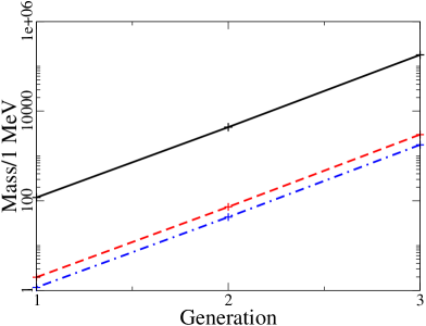
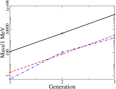
  (a)	(b)
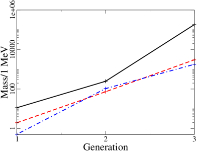
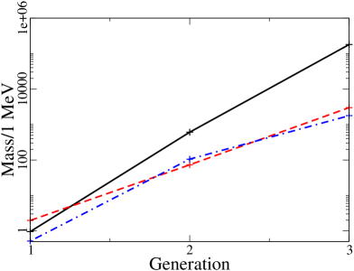
  (c)	(d)

  Figure 7: The masses of U-quarks (solid line), D-quarks (dashed line) and charged leptons (dashed-dotted line) at the $Z^{0}$ scale for the three generations. Figure (d) shows the results for the choice of parameters D in tables 5 and 7, in good agreement with experiment. Figures (a), (b) and (c) show how that brane configuration may be continuously reached from an underlying Pati-Salam configuration by shifting of branes and Wilson line breaking (see text).

  In fig.7(d), the solid and dashed lines show the masses of U- and D-quarks masses respectively of the three generations as reproduced by model D in table 5. One can restore $SU(2)_{R}$ symmetry by setting $\delta^{(3)}={\tilde{\delta}}^{(3)}$ (fig.7(c)) and setting $\phi^{(3)}={\tilde{\phi}}^{(3)}$ (fig.7(b),(a)). Then one observes that the masses of U-quarks and D-quarks are proportional, as it should in a left-right symmetric model. One can also check that in this LR-symmetric limit the mixing disappears. Note also that one observes that this $SU(2)_{R}$ breaking is the cause for the observed inverted hierarchy $m_{up}<m_{down}$ as well as the appearance of mixing (and also CP-violation).

• One can easily obtain fermion mass hierarchies consistent with experimental data. However, getting substantial CP violation requires that there are several instanton numbers contributing significantly to the world-sheet instanton sum in eq.(3.2). This happens when the torus radii $R^{(2)}$ and $R^{(3)}$ are smaller than $M_{s}^{-1}$, otherwise only the first term contributes and CP-violation is suppressed. Note however that the radii $R^{(2)}$ and $R^{(3)}$ cannot be too small, since then the instanton sum diverges and the quantum piece of the Yukawa coupling becomes relevant. We have checked in all the numerical examples that the corresponding instanton sum converges. In most of the cases the terms in the sum eq. (3.2) become negligible for $|l_{2}|,|l_{3}|\geq 6$.

• The complex phases coming from Wilson lines not only may account for the observed CP-violation. In addition, they have important influence on the values of the masses of the lightest fermions. Recall that, e.g., as we mentioned in the previous section the symmetry points with $\epsilon^{(2)},\ \delta^{(3)},\ {\tilde{\delta}}^{(3)}\ =\ 0,\ 1/2$ give rise to massless fermions only if, in addition, one has real phases $\phi^{(2)},\ \phi^{(3)},\ \tilde{\phi}^{(3)}\ =\ 0,\ 1/2$. Thus, for non-vanishing complex phases these massless modes will get massive.

We conclude that one can reproduce in a rather satisfactory way the quark masses, mixings and CP-violation in terms of the present model. Note that we have not done a fully systematic search for ranges of parameters able to reproduce the experimental results and the choices shown in the tables are just possible examples. Some values of parameters are particularly successful, like the choice D in table 5. The values we found for $tg\beta$ vary in the range $10-74$ and the value for $h_{0}$ is of order one, as expected from our discussion at the end of section 3.

Although there are a number of free parameters, note that the brane location parameters $\epsilon$, $\delta$ and phases in almost all cases sit close to symmetry points. One may speculate that those parameters could be fixed by some symmetry in the dynamics which eventually determines the geometry of the brane configuration. One can consider an scenario in which all the branes are located on top of some symmetry point like, e.g., that in (4.11), (4.12), (4.13) and some (e.g., loop) corrections give rise to a small deviation from those values. In such scenario the number of free parameters would be essentially reduced to the geometric moduli and $tg\beta$.

A similar study can be done for charged leptons and Dirac neutrino masses. In fact, once fixed $\epsilon_{l}^{(2)}$ and $\delta_{l}^{(3)}$ (plus phases) to reproduce the charged lepton spectrum, Dirac neutrino masses as well as Dirac mixing angles and leptonic CP-violating phases are fixed, since the geometry of the whole brane configuration gets completely determined. This is a very interesting point. However, in the case of neutrino masses the structure of the Majorana mass for the right-handed neutrinos is very relevant. As we mentioned above, once some linear combinations of sneutrinos get a vev (which may be triggered by a FI-term), the $SU(3)\times SU(2)\times U(1)_{c}\times U(1)_{B-L}$ symmetry is broken to the SM group. One can also see that in the same process r.h. neutrinos get a mass [20]. The latter mechanism is somewhat different to the class of Yukawa couplings we are considering here. Thus we will present a complete analysis of the leptonic and neutrino sector in this class of models in a separate publication. Here we will contempt ourselves with the analysis of the charged leptonic sector. Again one can reproduce the observed spectrum of charged leptons in terms of the location parameters of the leptonic brane $d$, $\epsilon_{l}^{(2)}$ and $\epsilon_{l}^{(3)}$ (and phases). In addition, once we have adjusted the quark and charged lepton sector, the Dirac neutrino masses and (Dirac) neutrino mixing matrix as well as leptonic CP-phases are fixed. Table 7 shows some choices of the leptonic parameters (corresponding to the previous quark sector choices A-E) giving rise to the results in table 8. Of course, only the charged lepton masses are directly measured at present, and those can be adjusted remarkably well. As we said, the rest of the information is certainly relevant for the structure of physical neutrino masses and leptonic CP phases, but a knowledge of the r.h. Majorana masses should be first provided. Let us only mention that the leptonic CP-phases may be large in some cases and also that sometimes one of the Dirac neutrino masses may be essentially vanishing. That happens, for instance, in model D because one sits on the point $(\delta_{l}^{(3)},\phi_{l}^{3})=(1/2,1/2)$, giving a vanishing column in the Dirac neutrino mass matrix. The corresponding sneutrino may then acquire a large vev (breaking (B-L)) without giving rise to a large mass term of type $HL$. This large vev would then give rise to large Majorana masses for all r.h. neutrinos, and a standard seesaw mechanism could then be at work.

We also find that the brane configurations able to reproduce in addition the observed spectrum of charged leptons may be understood as a deformation of a Pati-Salam symmetric configuration. As we said, if the leptonic brane sits on top of the baryonic stack (i.e., $\epsilon_{l}^{(2)}=\epsilon^{(2)}$ and $\epsilon_{l}^{(3)}=\epsilon^{(3)}$) the gauge symmetry is further enhanced to a full Pati-Salam symmetry $SU(4)\times SU(2)_{L}\times SU(2)_{R}$. Numerically we find (modulo 1/3) $\epsilon_{l}^{(2)}-\epsilon^{(2)}$$\simeq\delta_{l}^{(3)}-\delta^{(3)}\simeq 0.04-0.09$ indicating that the brane configuration able to reproduce the quark masses and mixings as well as the charged lepton masses may be considered as a deformation of a brane configuration leading to a Pati-Salam $SU(4)$ symmetry . This is again illustrated in fig.7. In fig.7(a) we have set $\epsilon^{(2)}=\epsilon_{l}^{(2)},\epsilon^{(3)}=\epsilon_{l}^{(3)}$ and also equal phases. Then the masses for D-quarks and charged leptons become proportional. In fact in the PS limit they should be equal at the string scale, but recall that we have allowed for different original values for $h_{0}$ and $h_{0}^{l}$, which could take in to account e.g., the renormalization group running from the string scale to the $Z^{0}$ scale.

Model	$h_{l}$	$\epsilon_{l}^{(2)}$	${\tilde{\delta}}_{l}^{(3)}$	$\phi_{l}^{(2)}$	$\phi_{l}^{(3)}$
A	0.684	0.35	0.0011	0.35	0.3104
B	0.43	0.4	0.155	0.23	0.29
C	1.51	0.17	0.03	0.47	0.38
D	0.166	0.499	0.508	0.1845	0.25
E	0.141	0.0	0.06	0.06	0.14

Table 7: Choices for the leptonic parameters corresponding to the ones in table 5 and leading to the results in table 8.

Model	$m_{e}$	$m_{\mu}$	$m_{\tau}$	$m_{\nu_{e}}$	$m_{\nu_{\mu}}$	$m_{\nu_{\tau}}$	$|V^{l}_{12}|$	$|V^{l}_{23}|$	$|V^{l}_{13}|$	$J_{l}$
A	0.512	105.66	1777	18.15	3.615	124.77	0.127	0.098	0.0002	$1.16\times 10^{-6}$
B	0.516	105.59	1777	309.5	4.683	83.95	0.052	0.228	0.021	$15.3\times 10^{-5}$
C	0.513	105.48	1777	1.90	1.698	160.22	0.021	0.057	0.0018	$5.7\times 10^{-7}$
D	0.516	105.52	1777	0.0	0.652	229.45	0.200	0.0648	0.0232	$5.9\times 10^{-7}$
E	0.511	105.56	1777	35.72	5.989	82.27	0.009	0.128	0.0044	$1.39\times 10^{-6}$

Table 8: Charged lepton and Dirac neutrino masses, mixing angles and (leptonic) Jarlskog invariant at the $Z^{0}$ scale for the model parameters of tables 5 and 7. All masses are given in MeV except for the two heaviest (Dirac) neutrino masses which are given in GeV.

5 Final comments and conclusions

A number of comments are in order:

• A few words about the particular brane configuration analyzed. For the comparison with experimental data we have considered a new D6-brane configuration which is particularly simple. At the local level the model has ${\cal N}=1$ SUSY and the MSSM chiral spectrum. It has the minimal Higgs sector of the MSSM and the $\mu$-parameter is governed by both the distance between the branes $b$ and $c$ and their relative Wilson line in the first torus. The gauge group is that of the SM plus an extra $U(1)$ familiar from left-right symmetric models. The latter may be broken spontaneously by a right-handed sneutrino vev, as explained in ref.[20]. If this configuration of D6-branes is wrapping a 6-torus, there are in addition adjoint scalars and fermions with respect to the gauge group, which would become massive after SUSY breaking. Let us remark that Type II string theory models with D-branes like this have consistency constraints from the cancellation of the Ramond-Ramond (RR) tadpoles. Specifically, the theory has certain antisymmetric fields under which D-branes (and orientifold planes) are charged. Tadpole conditions come from imposing that the overall RR-charges of the D-brane configuration vanishes. In the example considered in the text the D-brane configuration does not cancel by itself the RR-tadpoles. Thus in order to cancel RR-tadpoles there should be further D-branes in the model. Since however, the SM brane configuration is anomaly-free, the extra branes will have vanishing intersection numbers with the SM branes, i.e., they will not give rise to extra chiral massless modes, being some sort of ‘hidden sector’ in the model [20]. One can also check that in the simple toroidal case the complete D-brane configuration including the SM branes and the extra D-branes is necessarily non-SUSY [12, 20]. Thus one would be forced to lower the string scale (by making some compact volume large [39] ) in order to avoid a gauge hierarchy [13, 26] . Alternatively one could consider fully ${\cal N}=1$ SUSY extensions of this model, which is anyway ${\cal N}=1$ supersymmetric locally. In particular it would be interesting to see whether one can embed this very simple brane configuration into a fully ${\cal N}=1$ SUSY model as in refs.[18, 27].

• Irrespective of its construction as a string model, one may consider the brane configuration itself, with the fermions and Higgs fields at intersections, as a phenomenologically viable model for the understanding of quark and lepton masses and CP violation. The idea would be that analogously simple D-brane configurations incorporating similar mechanisms and symmetries could possibly be present in large classes of models with D6-branes wrapping cycles on compact manifolds (like, e.g., a Calabi-Yau). Note in this respect that the size of the string scale, either high or low, has no relevance for the computation of the Yukawa couplings. Thus our Yukawa coupling formulae may be applicable to both low string models and more conventional models with the string scale of order the GUT scale. We have seen, however, that in this toroidal example the size of the second and third tori have to be of order of the string scale in order to adjust the fermion spectrum data.

• The explicit formulae for Yukawa couplings provide a new laboratory for the understanding of the structure of fermion masses. Some properties of these formulae include possibilities phenomenologically explored previously. Thus for example, our Yukawa couplings depend on the brane location parameters, the $\epsilon$’s. Those correspond to vacuum expectation values of adjoints under the full gauge group (including $U(1)$’s). Expanding our formulae on the $\epsilon$-parameters would give rise to non-renormalizable couplings of the form $H\psi_{R}\psi_{L}(adjoint)^{n}$. This kind of couplings have been used since a long time in attempts to understand the SM Yukawa couplings. Unification symmetries like GUT’s have also played an important role in previous analysis. In the specific example studied in detail a Pati-Salam symmetry $SU(4)\times SU(2)_{L}\times SU(2)_{R}$ is underlying the brane configuration. The present scheme has also some analogies with the structure of Yukawa couplings in heterotic ${\bf Z}_{N}$ orbifold models [8, 9], in which fermions and Higgs multiplets located at different fixed points interact via world-sheet instanton effects. This is also somewhat analogous to recent attempts [37] to understand the fermion spectrum in terms of extra dimension models in which the fermions have different locations (with, e.g., a Gaussian wave function) and the different wave function overlap with the Higgs field determines the structure of Yukawa couplings.

• Other property that we find is the presence of accidental (approximate) global (e.g., $SU(2)$) symmetries in the structure of Yukawa couplings . For some geometrically symmetric brane locations some of the triangles formed by the branes become identical. At those locations (and for real phases) two columns and/or rows of the fermion mass matrices become identical, signalling the presence of a massless fermion. The numerical analysis shows that in order to have sufficiently light up- and down-quarks the branes should be close to these symmetry points. We have also found that for other symmetric brane configurations there are cancellations between different instanton contributions giving rise to vanishing columns and/or rows in the mass matrices. It is the interplay of these two effects which turns out to be able to reproduce the observed fermion spectrum, rather than any exponential suppression of the lightest fermions.

• One of the nice insights of the present construction is that of the origin of CP-violation. In our constructions complex phases appear associated to the generic presence of non-vanishing Wilson lines of the $U(1)$’s of the model. We believe this is rather general and is not specific to our particular constructions. This means that the origin of CKM CP-violation is an open string effect, i.e., it is associated to the D-branes, rather than to the bulk fields. This is interesting because if promoted to a fully ${\cal N}=1$ setting, it may provide a solution to the supersymmetry CP-problem, that is, why the phases of soft terms are so small (which is required from EDMN limits) compared to the CKM phase (for some recent work on CP-violation in string models see, e.g., [40] and for the same issue in extra dimensions see [41]). If soft terms physics comes from the bulk (closed string) gravitational sector, they may be all real without affecting CKM mixing. In other words CKM CP-violation would come from the open string sector and soft-term CP-violation from the closed string (bulk) sector.

In summary, we have shown how simple configurations of D-branes wrapping a compact space may give a good quantitative description of quark masses and mixing angles as well as CP-violation and charged lepton masses. We believe that the approach is more general than the particular example numerically explored since all realistic D-brane models constructed up to now may be re-expressed as coming from D6-branes wrapping cycles in some compact space [26].

One of the nice features of this approach is that one can obtain simple explicit formulae for each Yukawa as a sum over world-sheet instanton contributions. A non-vanishing value for $U(1)$ Wilson lines lies at the origin of complex phases and CP violation. Symmetric configurations of the branes lead to approximate symmetries of the fermion mass matrices, giving rise to particular patterns in the fermion spectrum. Interestingly enough our analysis shows that the experimental data is consistent with the existence of an underlying Pati-Salam symmetry which is broken by shifting of the brane locations (adjoint Higgsing in the field theory language). This shifting is also the cause of the reversion of the up-down hierarchy (i.e., $m_{up}<m_{down}$), the presence of CKM mixing and CP violation. It is certainly worthwhile to study the neutrino mass spectrum from this perspective. We hope to report on this issue in the near future.

Acknowledgements

We are grateful to G. Aldazábal, G. Honecker, C. Kokorelis, F. Quevedo, R. Rabadán and A. Uranga for useful discussions. The research of D.C. and F.M. was supported by the Ministerio de Educación, Cultura y Deporte (Spain) through FPU grants. This work is partially supported by CICYT (Spain) and the European Commission (RTN contract HPRN-CT-2000-00148).

References

-
[1]
H. Fritzsch and Z. z. Xing,
“Mass and flavor mixing schemes of quarks and leptons,”
Prog. Part. Nucl. Phys. 45, 1 (2000),
hep-ph/9912358.
F. J. Gilman and Y. Nir, “Quark Mixing: The CKM Picture,” Ann. Rev. Nucl. Part. Sci. 40, 213 (1990). - [2] K. Hagiwara et al. [Particle Data Group Collaboration], “Review Of Particle Physics,” Phys. Rev. D 66, 010001 (2002), http://pdg.lbl.gov/pdg.html.
- [3] C. Jarlskog, “Commutator Of The Quark Mass Matrices In The Standard Electroweak Model And A Measure Of Maximal CP Violation,” Phys. Rev. Lett. 55, 1039 (1985).
-
[4]
R. Gatto, G. Sartori and M. Tonin,
“Weak Selfmasses, Cabibbo Angle, And Broken ,”
Phys. Lett. B 28, 128 (1968).
N. Cabibbo and L. Maiani, “Dynamical Interrelation Of Weak, Electromagnetic And Strong Interactions And The Value Of Theta,” Phys. Lett. B 28, 131 (1968).
R. J. Oakes, “ Breaking And The Cabibbo Angle,” Phys. Lett. B 29, 683 (1969). -
[5]
C. D. Froggatt and H. B. Nielsen,
“Hierarchy Of Quark Masses, Cabibbo Angles And CP Violation,”
Nucl. Phys. B 147, 277 (1979).
Z. G. Berezhiani, “The Weak Mixing Angles In Gauge Models With Horizontal Symmetry - A New Approach To Quark And Lepton Masses,” Phys. Lett. B 129, 99 (1983).
M. Leurer, Y. Nir and N. Seiberg, “Mass matrix models,” Nucl. Phys. B 398, 319 (1993), hep-ph/9212278. -
[6]
L. E. Ibáñez and G. G. Ross,
“Fermion Masses And Mixing Angles From Gauge Symmetries,”
Phys. Lett. B 332, 100 (1994),
hep-ph/9403338.
P. Binétruy and P. Ramond, “Yukawa textures and anomalies,” Phys. Lett. B 350, 49 (1995), hep-ph/9412385. - [7] S. Raby, “Introduction to theories of fermion masses,” hep-ph/9501349.
-
[8]
S. Hamidi and C. Vafa,
“Interactions On Orbifolds,”
Nucl. Phys. B 279, 465 (1987).
L. J. Dixon, D. Friedan, E. J. Martinec and S. H. Shenker, “The Conformal Field Theory Of Orbifolds,” Nucl. Phys. B 282, 13 (1987). -
[9]
L. E. Ibáñez,
“Hierarchy Of Quark - Lepton Masses
In Orbifold Superstring Compactification,”
Phys. Lett. B 181, 269 (1986).
J. A. Casas, F. Gómez and C. Muñoz, “Complete structure of Yukawa couplings,” Int. J. Mod. Phys. A 8, 455 (1993), hep-th/9110060. “Fitting the quark and lepton masses in string theories,” Phys. Lett. B 292, 42 (1992), hep-th/9206083. - [10] G. Aldazábal, L. E. Ibáñez, F. Quevedo and A. M. Uranga, “D-branes at singularities: A bottom-up approach to the string embedding of the standard model,” JHEP 0008, 002 (2000), hep-th/0005067.
-
[11]
J. Lykken, E. Poppitz and S. Trivedi,
“Branes with GUTs and supersymmetry breaking,”
Nucl. Phys. B 542, 31 (1999),
hep-th/9806080.
Z. Kakushadze and S. H. Tye, “Three generations in type I compactifications,” Phys. Rev. D 58, 126001 (1998), hep-th/9806143.
I. Antoniadis, E. Dudas and A. Sagnotti, “Brane supersymmetry breaking,” Phys. Lett. B 464, 38 (1999), hep-th/9908023.
G. Aldazábal and A. M. Uranga, “Tachyon-free non-supersymmetric type IIB orientifolds via brane-antibrane systems,” JHEP 9910, 024 (1999), hep-th/9908072.
G. Aldazábal, L. E. Ibáñez and F. Quevedo, “Standard-like models with broken supersymmetry from type I string vacua,” JHEP 0001, 031 (2000), hep-th/9909172. “A D-brane alternative to the MSSM,” JHEP 0002, 015 (2000), hep-ph/0001083.
A. M. Uranga, “From quiver diagrams to particle physics,” hep-th/0007173.
D. Bailin, G. V. Kraniotis and A. Love, “Supersymmetric standard models on D-branes,” Phys. Lett. B 502, 209 (2001), hep-th/0011289.
D. Berenstein, V. Jejjala and R. G. Leigh, “The Standard Model on a D-brane,” Phys. Rev. Lett. 88, 071602 (2002), hep-ph/0105042.
L. L. Everett, G. L. Kane, S. F. King, S. Rigolin and L. T. Wang, “Supersymmetric Pati-Salam models from intersecting D-branes,” Phys. Lett. B 531, 263 (2002), hep-ph/0202100.
L. F. Alday and G. Aldazábal, “In quest of “just” the Standard Model on D-branes at a singularity,” JHEP 0205, 022 (2002), hep-th/0203129.
I. Antoniadis, E. Kiritsis, J. Rizos and T. N. Tomaras, “D-branes and the Standard Model,” arXiv:hep-th/0210263. - [12] R. Blumenhagen, L. Görlich, B. Körs and D. Lüst, “Noncommutative compactifications of type I strings on tori with magnetic flux”, JHEP 0010, 006 (2000), hep-th/0007024. “Magnetic flux in toroidal type I compactification,” Fortsch. Phys. 49, 591 (2001), hep-th/0010198.
- [13] G. Aldazábal, S. Franco, L. E. Ibáñez, R. Rabadán and A. M. Uranga, “D = 4 chiral string compactifications from intersecting branes,” J. Math. Phys. 42, 3103 (2001), hep-th/0011073.
- [14] G. Aldazábal, S. Franco, L. E. Ibáñez, R. Rabadán and A. M. Uranga, “Intersecting Brane Worlds,” JHEP 0102, 047 (2001), hep-ph/0011132.
- [15] R. Blumenhagen, B. Körs and D. Lüst, “Type I strings with F- and B-flux,” JHEP 0102, 030 (2001), hep-th/0012156.
- [16] L. E. Ibáñez, F. Marchesano and R. Rabadán, “Getting just the Standard Model at Intersecting Branes,” JHEP 0111, 002 (2001), hep-th/0105155.
- [17] R. Blumenhagen, B. Körs, D. Lüst and T. Ott, “The standard model from stable intersecting brane world orbifolds,” Nucl. Phys. B 616, 3 (2001), hep-th/0107138.
- [18] M. Cvetič, G. Shiu and A. M. Uranga, “Three-family supersymmetric standard like models from intersecting branes,” Phys. Rev. Lett. 87, 201801 (2001), hep-th/0107143. “Chiral four-dimensional N = 1 supersymmetric type IIA orientifolds from intersecting branes,” Nucl. Phys. B 615, 3 (2001), hep-th/0107166.
-
[19]
D. Bailin, G. V. Kraniotis and A. Love,
“Standard-like models from intersecting D4-branes,”
Phys. Lett. B 530, 202 (2002),
hep-th/0108131.
“Standard-like models from intersecting D5-branes,”
hep-th/0210219.
D. Bailin, “Standard-like models from D-branes,” hep-th/0210227. - [20] D. Cremades, L. E. Ibáñez and F. Marchesano, “SUSY Quivers, Intersecting Branes and the Modest Hierarchy Problem,” JHEP 0207, 009 (2002), hep-th/0201205. “Intersecting Brane Models of Particle Physics and the Higgs Mechanism,” JHEP 0207, 022 (2002), hep-th/0203160.
- [21] G. Honecker, “Non-supersymmetric orientifolds with D-branes at angles,” Fortsch. Phys. 50, 896 (2002), hep-th/0112174. “Intersecting brane world models from D8-branes on type IIA orientifolds,” JHEP 0201, 025 (2002), hep-th/0201037.
- [22] C. Kokorelis, “GUT model hierarchies from intersecting branes,” JHEP 0208, 018 (2002), hep-th/0203187. “New standard model vacua from intersecting branes,” JHEP 0209, 029 (2002), hep-th/0205147. “Exact standard model compactifications from intersecting branes,” JHEP 0208, 036 (2002), hep-th/0206108. “Exact standard model structures from intersecting D5-branes,” hep-th/0207234. “Deformed intersecting D6-brane GUTs. I,” JHEP 0211, 027 (2002), hep-th/0209202.
- [23] J. R. Ellis, P. Kanti and D. V. Nanopoulos, “Intersecting branes flip SU(5),” hep-th/0206087.
- [24] D. Cremades, L. E. Ibáñez and F. Marchesano, “Standard model at intersecting D5-branes: Lowering the string scale,” Nucl. Phys. B 643, 93 (2002), hep-th/0205074.
- [25] R. Blumenhagen, V. Braun, B. Körs and D. Lüst, “Orientifolds of K3 and Calabi-Yau manifolds with intersecting D-branes,” JHEP 0207, 026 (2002), hep-th/0206038.
- [26] A. M. Uranga, “Local models for intersecting brane worlds,” JHEP 0212, 058 (2002), hep-th/0208014.
- [27] R. Blumenhagen, L. Görlich and T. Ott, “Supersymmetric intersecting branes on the type IIA orientifold,” hep-th/0211059.
- [28] L. E. Ibáñez, “Standard Model Engineering with Intersecting Branes,” hep-ph/0109082.
-
[29]