HIP-2002-61/TH
DO-TH 02/20
hep-ph/0212047
Effects of Universal Extra Dimensions on
$B^{0}-\bar{B^{0}}~{}~{}$Mixing

Abstract

We study contributions coming to $\Delta m_{B}$ from one or more universal extra dimensions (UED) in which all the Standard Model fields can propagate. In the model with a single UED, the box diagrams for mixing are convergent and therefore insensitive to the cutoff scale of the theory. In the case of two UEDs, the result is not very sensitive to the cut-off scale due to GIM mechanism. Within the present range of the parameters at $1\sigma$ level, the lower bound on the compactification scale $1/R$ has been estimated to be 165 GeV for one UED and 280 GeV for two UEDs. The bound increases drastically if one can have a better determination of the $B$ meson decay constant $f_{B}$ and the QCD correction parameter $B_{B}$. For example, it rises to 740 GeV (for one UED) if the error (at $1\sigma$) in the determination of $f_{B}\sqrt{B_{B}}$ from quenched lattice calculation is reduced to one-third from its present value. The UED contributions to the $K$ system are strongly suppressed.

PACS number(s): 11.25.Mj, 12.15.Ff, 14.40.Nd

Inspired by the string theories, a possible solution to the hierarchy problem of the Standard Model (SM) may be the higher dimensional scenarios. These scenarios get additional motivation from the potential to solve some of the open problems of the SM: gauge coupling unification [1], supersymmetry breaking [2], neutrino mass generation [3], and the explanation of fermion mass hierarchies [4]. The observation of four dimensional world in our everyday life ensures that the extra dimensions are compactified. The simplest way is to compactify them on a circle of a radius $R$ ($S^{1}$). A nice feature of these theories is that the compactification radius can be large so that $1/R$ can be as low as a few hundreds of GeV [2, 5]. One might argue that in the most natural framework all the SM fields should be allowed to propagate in the extra dimensions. Care, however, must be taken to obtain chiral fermions in four dimensions (4D) from such universal extra dimension (UED) models.

In this letter we confine ourselves to the UED model formulated in [6]. In 4D effective theory, the existence of these extra dimensions are felt by the appearance of towers of heavy Kaluza-Klein (KK) states having masses quantised in units of the compactification scale $1/R$. The key feature of UED models is the conservation of momentum in extra dimensions which leads to KK number conservation in the effective 4D theory. Such theories naturally lead to the existence of a lightest KK particle which is a viable dark matter candidate [7]. One should note in this context that orbifolding, which is necessary to forbid wrong-chirality fermions at the lowest level, generates KK number violating interactions through boundary terms [8, 9]. Though these interactions have interesting phenomenological implications in the decays of such KK modes, we put them to be equal to zero by hand and do not consider them any further in our study of the virtual effects of those modes. Consequently in our calculations, there are no vertices which violate the KK number conservation. This forbids production of isolated KK particles at colliders and tree level contributions to the electroweak observables. In the non-universal case, where the fermions (and maybe some of the bosons) are confined to a 4D brane, the presence of a localising delta function in the Lagrangian permits KK number violating couplings, which is not true for the UED models, and hence none of the existing bounds on non-universal extra dimensional models from single KK productions at colliders [10] and from tree as well as loop level electroweak constraints [11] are applicable for UEDs. In UED, apart from the direct KK pair production at colliders [12], one may get indirect bound on the compactification scale $1/R$ from the virtual effects of KK modes at loop level [6, 13, 14, 15]. It is natural to look on processes which are sensitive to radiative corrections even in the absence of KK modes in order to study the dominant loop effects induced by the exchange of them. In the SM, the most important loop effects are those enhanced by the heavy top quark mass. Thus one may get valuable information on the size of the extra dimension through the one loop KK mode contributions to the processes, $Z\to b{\bar{b}}$ [6], $b\to s\gamma$ [15] and $B^{0}-\bar{B^{0}}$ mixing. The lower bound on the compactification scale ($1/R$) from collider phenomenology [12], Higgs physics [14], electroweak precision measurements [6], and flavour changing process $b\to s\gamma$ [15] has been estimated to lie between 200 and 500 GeV.

In this letter, we mainly address the effects of only one spatial UED at the one-loop level to $B^{0}-\bar{B^{0}}$ mixing. The bound on the compactification scale is derived taking into account all input uncertainties (and we also show what happens if these uncertainties come down) and hence can be regarded as a robust one. A brief qualitative discussion for more than one extra dimension is also presented, and we comment on the $K$ system too. As a starting point, we consider the relevant part of the five dimensional ($5D$) Lagrangian:

$${\cal L}_{5}(x,y)=i{\bar{Q}}\Gamma^{M}D_{M}Q+\lambda^{U}_{5}{\bar{Q}}U(i\sigma_{2}H^{*})+\lambda_{5}^{D}{\bar{Q}}DH+h.c.$$ (1)

Here $M$ (1 to 5) is the Lorentz index. The covariant derivative $D_{M}$ can be expressed as

$$D_{M}=\partial_{M}+i\sum_{i=1}^{3}g_{5}^{i}T_{i}^{a}A_{iM}^{a},$$ (2)

where $g_{5}^{i}$s are the $5D$ coupling constants associated with the SM gauge group $SU(3)_{c}\times SU(2)_{L}\times U(1)_{Y}$, and $T_{i}^{a}$s are the corresponding generators. The parameters $\lambda_{5}^{U}$ and $\lambda_{5}^{D}$ are the 5D Yukawa couplings. The 5D Dirac matrices are $\Gamma^{M}\equiv(\gamma^{\mu},i\gamma^{5})$ (see, e.g., [16]) and $y$ denotes the coordinate along the extra dimension. The fields $Q$, $U$ and $D$, all functions of $x^{\mu}$ and $y$, describe 5D generic quark doublet, up type quark singlet, and down type quark singlet, respectively. Unlike in the Standard Model, they have both chiralities, and are of vector type. The field $H$ is the 5D Higgs doublet, and the generic 5D gauge bosons for each gauge group are denoted by $A_{iM}^{a}$. The component of the gauge bosons along the extra dimension is the pseudoscalar $A_{i5}$. In order to derive the 4D Lagrangian we must expand the five dimensional fields into their KK modes. To project out the zero modes of the wrong chirality (i.e., $Q_{R}$, $U_{L}$, and $D_{L}$) and the fifth component of the gauge field, $A_{5}^{i}$, the fifth dimension $y$ is compactified on an $S^{1}/Z_{2}$ orbifold ($Z_{2}:y\to-y$). The KK decompositions of the 5D fields are:

$$H(x,y) = {1\over{\sqrt{2\pi R}}}\left\{H^{(0)}(x)+\sqrt{2}\sum_{n=1}^{\infty}H^{(n)}(x)\cos(ny/R)\right\}$$

$$A_{i\mu}(x,y) = {1\over{\sqrt{2\pi R}}}\left\{A_{i\mu}^{(0)}(x)+\sqrt{2}\sum_{n=1}^{\infty}A_{i\mu}^{(n)}(x)\cos(ny/R)\right\}$$

$$A_{i5}(x,y) = {1\over{\sqrt{\pi R}}}\sum_{n=1}^{\infty}A_{i5}^{(n)}(x)\sin(ny/R)$$

$$Q(x,y) = {1\over{\sqrt{2\pi R}}}\left\{Q_{L}^{(0)}(x)+\sqrt{2}\sum_{n=1}^{\infty}\left[Q_{L}^{(n)}(x)\cos(ny/R)+Q_{R}^{(n)}(x)\sin(ny/R)\right]\right\}$$

$$U(x,y) = {1\over{\sqrt{2\pi R}}}\left\{U_{R}^{(0)}(x)+\sqrt{2}\sum_{n=1}^{\infty}\left[U_{R}^{(n)}(x)\cos(ny/R)+U_{L}^{(n)}(x)\sin(ny/R)\right]\right\}$$

$$D(x,y) = {1\over{\sqrt{2\pi R}}}\left\{D_{R}^{(0)}(x)+\sqrt{2}\sum_{n=1}^{\infty}\left[D_{R}^{(n)}(x)\cos(ny/R)+D_{L}^{(n)}(x)\sin(ny/R)\right]\right\}$$ (3)

Here the factor of $\sqrt{2}$ is due to the different normalizations of the zero and higher modes in the KK tower; it would not have been there if we run the sum over both positive and negative values of the KK number $n$. The fields which are even under the $Z_{2}$ orbifold symmetry have zero modes, and they correspond to the SM particles in usual four dimensions. Fields which are odd under $Z_{2}$ do not have zero modes and hence are absent in the SM spectrum.

Using the KK expansions of the 5D fields and integrating out the 5D Lagrangian over the extra dimension $y$, the effective 4D Lagrangian is obtained. Apart from the usual mass term coming from the vacuum expectation value of the zero-mode Higgs, KK excitations also receive masses from the kinetic energy term in the 5D Lagrangian. The mass of the $n$-th level KK particle, where $n$ is the KK excitation number that quantises the momentum along the extra dimension $y$, is given by $m_{n}^{KK}=\sqrt{m_{0}^{2}+m_{n}^{2}}$ where $m_{0}$ is the zero mode mass and $m_{n}=n/R$. Thus the KK spectrum at each excitation level is nearly degenerate except for the heavy SM particles ($t,W,Z,h$). This degeneracy is removed by the radiative corrections of KK mode masses [8] which play an important role in collider phenomenology. However, this has only a negligible effect on our results, and so we can take the KK excitations of all the light particles to be degenerate. The couplings $g_{5}^{i}$, $\lambda_{5}^{U}$ and $\lambda_{5}^{D}$ are dimensionful and they have to be rescaled as $g^{i}=g_{5}^{i}/\sqrt{2\pi R}$, $\lambda^{U}=\lambda_{5}^{U}/\sqrt{2\pi R}$ and $\lambda^{D}=\lambda_{5}^{D}/\sqrt{2\pi R}$ to obtain the proper dimensionless SM couplings.

The zero mode and the KK Higgs doublets can be written as

$$\pmatrix{\phi^{(0)+}\cr{1\over\sqrt{2}}(v+h^{(0)}+i\chi^{(0)})},{\quad}\pmatrix{\phi^{(n)+}\cr{1\over\sqrt{2}}(h^{(n)}+i\chi^{(n)})}.$$ (4)

Here $h^{(n)}$s are neutral Higgs KK excitations. The charged scalars $\phi^{\pm(n)}$ combining with the $W^{\pm 5(n)}$ form longitudinal components of the $W^{\pm(n)}_{\mu}$. The orthogonal combinations yield physical charged Higgs KK tower. Goldstone KK modes for $W^{\pm(n)}$ are

$$G^{\pm(n)}={{m_{n}W^{\pm(n)}_{5}\pm im_{W}\phi^{\pm(n)}}\over{\sqrt{m_{n}^{2}+m_{W}^{2}}}}$$ (5)

and the physical charged Higgs KK tower is

$$H^{\pm(n)}={{m_{n}\phi^{\pm(n)}\pm im_{W}W^{\pm(n)}_{5}}\over{\sqrt{m_{n}^{2}+m_{W}^{2}}}}.$$ (6)

Similarly, the $\chi^{(n)}$ together with the $Z^{5(n)}$ generate additional physical neutral Higgs tower and longitudinal components of the $Z_{\mu}^{(n)}$. However, they do not contribute to our study and have consequently not been discussed further. In the unitary gauge which we will use for our calculation, Goldstone KK modes are eaten up by the longitudinal parts of the gauge boson KK modes. The fields $W_{\mu}^{\pm(n)}$ and $H^{\pm(n)}$ have the same mass as $m_{W,n}=\sqrt{m_{n}^{2}+m_{W}^{2}}$, since we are neglecting the loop corrections to the KK modes.

Rotating the quark fields to the mass eigenbasis from the weak eigenbasis is similar to that in the SM and leads to a universal CKM matrix, same for all KK levels. Furthermore, one generally performs a chiral transformation to get the 4D mass terms with the correct sign:

$$\pmatrix{U^{(n)}\cr Q^{(n)}}=\pmatrix{-\gamma_{5}\cos{\alpha_{n}}&\sin{\alpha_{n}}\cr\gamma_{5}\sin{\alpha_{n}}&\cos{\alpha_{n}}}\pmatrix{U^{(n)^{\prime}}\cr Q^{(n)^{\prime}}}$$ (7)

with the mixing angle $\tan{2\alpha_{n}}=m_{q}/m_{n}$. Obviously, the mixing angles can be neglected for all quarks except the top.

For $B^{0}-\bar{B^{0}}$ mixing, we need the vertices involving one zero mode and two non zero KK modes, $W^{+(n)}{\bar{d}}u_{i}^{(n)}$, $W^{-(n)}{\bar{u}}_{i}^{(n)}b$, $H^{+(n)}{\bar{d}}u_{i}^{(n)}$ and $H^{-(n)}{\bar{u}}_{i}^{(n)}b$, to calculate the relevant box diagrams in UED. The vertices $H^{+(n)}{\bar{d}}u_{i}^{(n)}$ and $H^{-(n)}{\bar{u}}_{i}^{(n)}b$ have two parts, one coming from $\phi^{\pm(n)}$ interactions, while other part from $W_{5}^{\pm(n)}$. All these relevant vertices are obtained from the four dimensional Lagrangian $\int_{-\pi R}^{\pi R}{\cal L}_{5}(x,y)dy$. The 5D integrations ${1\over{(2\pi R)^{3/2}}}\int_{-\pi R}^{\pi R}2\cos^{2}(ny/R)dy$ and ${1\over{(2\pi R)^{3/2}}}\int_{-\pi R}^{\pi R}2\sin^{2}(ny/R)dy$ are just $1\over\sqrt{2\pi R}$, and combining them with $g_{5}^{i}$’s we get just the ordinary 4D gauge couplings $g^{i}$. Thus these vertices are exactly identical to the SM ones in weak basis. The only point to note is that the mass terms appearing in the Yukawa couplings of the $\phi^{\pm(n)}$ (relevant for charged Higgs KK mode interactions) are the zero-mode and not the excited level masses of the corresponding quarks. The box diagrams relevant for $B^{0}-\bar{B^{0}}$ mixing in UED are shown in Fig. 1, to which one must add the crossed diagrams with intermediate boson and quark lines interchanged. In the case of SM, the box diagram is mediated only by the exchange of the $W$ boson in the unitary gauge, while in the UED case, the exchange of the KK modes of the charged Higgs will give extra diagrams in addition to that by the KK excitations of $W$.

Figure 1: UED contributions to the box diagrams for $B^{0}-\bar{B^{0}}$ mixing.

The UED contributions to the effective Hamiltonian for $\Delta B=2$ transitions responsible for $B^{0}-\bar{B^{0}}$ mixing, which come from the box diagrams shown in Fig. 1, are

$${\cal H}_{\rm eff}^{UED}={{G_{F}^{2}\lambda_{t}^{2}}\over{4\pi^{2}}}\left({m_{W}^{4}\over{m_{W,n}^{2}}}\right)\left({\bar{d}}\gamma_{\mu}{{(1-\gamma_{5})}\over 2}b\right)^{2}\sum_{n=1}^{\infty}\left[S(X_{t},X_{t})+S(X_{u},X_{u})-2S(X_{t},X_{u})\right]$$ (8)

where

$$S(X_{i},X_{j})=S^{WW}(X_{i},X_{j})+S^{HW}(X_{i},X_{j})+S^{HH}(X_{i},X_{j})$$ (9)

with $X_{i}=m_{i,n}^{2}/m_{W,n}^{2}$ and $\lambda_{i}=V_{ib}V_{id}^{*}$. The functions $S^{WW}(X_{i},X_{j})$ come from the box diagram mediated by two excited $W$s and is of the same form as in the SM [17] with the appropriate modification of masses:

$$S^{WW}(X_{i},X_{j})=X_{i}X_{j}{\Big{\{}}{\Big{[}}{1\over 4}+{3\over 2}{1\over{1-X_{i}}}-{3\over 4}{1\over{(1-X_{i})^{2}}}{\Big{]}}{\ln{X_{i}}\over{X_{i}-X_{j}}}+(X_{i}\leftrightarrow X_{j})-{3\over 4}{1\over{(1-X_{i})(1-X_{j})}}{\Big{\}}}.$$ (10)

$S^{HH}(X_{i},X_{j})$ and $S^{HW}(X_{i},X_{j})$ are the contributions coming from the charged Higgs KK box and the mixed boxes (with one $W^{(n)}$ and one $H^{(n)}$) respectively:

$$S^{HW}(X_{i},X_{j}) = {x_{n}\over{(1+x_{n})^{2}}}(1-x_{i})(1-x_{j})\left[{F_{1}(X_{i},X_{j})\over 2}-2F_{2}(X_{i},X_{j})\right]$$ (11)

$$S^{HH}(X_{i},X_{j}) = {1\over{4(1+x_{n})^{2}}}(1+x_{i}x_{n})(1+x_{j}x_{n})F_{1}(X_{i},X_{j})$$ (12)

with $x_{i}=m_{i}^{2}/m_{W}^{2}$ and $x_{n}=m_{n}^{2}/m_{W}^{2}$. The functional forms of $F_{1}(X_{i},X_{j})$ and $F_{2}(X_{i},X_{j})$ are given by,

$$F_{1}(X_{i},X_{j}) = {{[X_{j}^{2}(1-X_{i})^{2}\log{X_{j}}-X_{i}^{2}(1-X_{j})^{2}\log{X_{i}}+(1-X_{j})(X_{j}-X_{i})(1-X_{i})]}\over{(1-X_{i})^{2}(1-X_{j})^{2}(X_{j}-X_{i})}}$$ (13)

$$F_{2}(X_{i},X_{j}) = {{[X_{j}(1-X_{i})^{2}\log{X_{j}}-X_{i}(1-X_{j})^{2}\log{X_{i}}+(1-X_{j})(X_{j}-X_{i})(1-X_{i})]}\over{(1-X_{i})^{2}(1-X_{j})^{2}(X_{j}-X_{i})}}$$ (14)

In the limit $X_{i}=X_{j}$, the expressions $S^{WW}(X_{i},X_{j})$, $F_{1}(X_{i},X_{j})$ and $F_{2}(X_{i},X_{j})$ become

$$S^{WW}(X_{i},X_{i}) = {{X_{i}(4-15X_{i}+12X_{i}^{2}-X_{i}^{3}-6X_{i}^{2}\ln{X_{i}})}\over{4(1-X_{i})^{3}}}$$ (15)

$$F_{1}(X_{i},X_{i}) = {{1-X_{i}^{2}+2X_{i}\log{X_{i}}}\over{(1-X_{i})^{3}}}$$

$$F_{2}(X_{i},X_{i}) = {{2-2X_{i}+(1+X_{i})\log{X_{i}}}\over{(1-X_{i})^{3}}}$$

In eq. (8), we have considered box diagrams with all combinations of the three excited up type quarks ($i,j=u,c,t$). The terms are then rearranged by eliminating $\lambda_{u}$ in favour of $\lambda_{c}$ and $\lambda_{t}$ using the unitarity relation and thus the GIM mechanism of the SM is restored. The terms containing $\lambda_{c}^{2}$ and $\lambda_{c}\lambda_{t}$ are $[S(X_{c},X_{c})+S(X_{u},X_{u})-2S(X_{c},X_{u})]$ and $[2S(X_{c},X_{t})-2S(X_{u},X_{t})+2S(X_{u},X_{u})-2S(X_{c},X_{u})]$ respectively and vanish as $X_{c}\simeq X_{u}\simeq{m_{n}^{2}/m_{W,n}^{2}}$.

The UED contribution to the mass difference for the $B^{0}$ mesons ($\Delta m_{B}$) is given by

$$(\Delta m_{B})^{UED}={{|\langle B^{0}|{\cal H}_{\rm eff}^{UED}|\bar{B^{0}}\rangle|}\over m_{B^{0}}}.$$ (16)

The matrix element for $\langle B^{0}|({\bar{d}}\gamma_{\mu}(1-\gamma_{5})b)({\bar{d}}\gamma^{\mu}(1-\gamma_{5})b)|{\bar{B^{0}}}\rangle$ is calculated in the usual vacuum insertion approximation, and we have

$$\langle B^{0}|({\bar{d}}\gamma_{\mu}(1-\gamma_{5})b)({\bar{d}}\gamma^{\mu}(1-\gamma_{5})b)|\bar{B^{0}}\rangle={8\over 3}B_{B}f_{B}^{2}m_{B}^{2}$$ (17)

which gives,

$$(\Delta m_{B})^{UED}={G_{F}^{2}\over{6\pi^{2}}}\sum_{n=1}^{\infty}{m_{W}^{4}\over{m_{W,n}^{2}}}|\lambda_{t}|^{2}[S(X_{t},X_{t})+S(X_{u},X_{u})-2S(X_{t},X_{u})]B_{B}f_{B}^{2}m_{B}\eta_{B},$$ (18)

where the bag factor, $B_{B}$, is introduced to parametrize all possible deviations from the vacuum saturation approximation. The quantity $B_{B}f_{B}^{2}$ has been evaluated from QCD studies on lattice. The next-to-leading order (NLO) short distance QCD correction is given by $\eta_{B}$.

Let us also comment on the case when one has more than one UED. The electroweak observables are known be convergent for one UED, but diverges when the number of UEDs is two or more [6]. The SU(3) gauge coupling also becomes nonperturbative at high scales for two UEDs, so one has to use a cut-off scale $M_{s}$ in the multi-TeV range upto which such perturbative calculations make sense. This means a natural truncation of the KK mode sum at $n=n_{s}$ ($n_{s}\sim M_{s}R$) where $R$ is the common compactification radius. The effect mainly arises due to a crowding of KK states for more than one UED. However, it is gratifying to note that the lower limit on $1/R$ is fairly insensitive to the exact value of $n_{s}$ since the terms which do not decouple vanish due to GIM cancellation.

Now we shall comment on the reliability of the parameters we need for $B^{0}-\bar{B^{0}}$ mixing. The short distance QCD corrections $\eta_{B}$ are well determined [18], while the long distance corrections are estimated to be small, unlike in the case of $K$-${\bar{K}}$ mixing. Major uncertainties come from quantities like $V_{td}$, $f_{B}$ and $B_{B}$. We have used the value of $f_{B}\sqrt{B_{B}}$ at a scale of order $m_{b}$ obtained by UKQCD collaboration [19] in quenched lattice calculation. In the widely used generalised Wolfenstein parametrisation of the CKM matrix, the CKM matrix elements are expressed in terms of the four parameters $\lambda$, $A$, $\bar{\rho}$ and $\bar{\eta}$. Of these, $\lambda$ and A are presently known at $1\%$ and $5\%$ levels respectively, whereas $\bar{\rho}$ and $\bar{\eta}$ are the least known CKM parameters. The uncertainty in $V_{td}$ is solely due to the broad allowed range in the $({\bar{\rho}},{\bar{\eta}})$ plane. However, one should note that since $\Delta m_{B}$ is affected by UED, the SM fit values of quantities like $V_{td}$, mainly determined from $B^{0}-\bar{B^{0}}$ mass difference, may not be used any further.

Parameter	$1\sigma$ level
$\lambda$	$0.221\pm 0.002$
$A$	$0.83\pm 0.02$
$\bar{\rho}$	$0.151\pm 0.057$
$\bar{\eta}$	$0.369\pm 0.032$
$|V_{td}|(\times 10^{3})$	$8.36\pm 0.55$
$f_{B}\sqrt{B_{B}}$	$(235{{+33}\atop{-41}})~{}~{}{\rm MeV}$

Table 1: The ranges of relevant parameters allowed by UUT at $1\sigma$ level from [21].

The models with UED do not have any new local operators beyond those already present in SM. In UED, the flavor changing transitions and CP violation are solely governed by the CKM matrix. Furthermore, these models do not contribute to inclusive and exclusive $K$ and $B$ decays due to the absence of KK number violating interactions. These properties specify the so-called universal unitarity triangle (UUT) scenario [20], which has been constructed from $|V_{ub}/V_{cb}|$, $\Delta m_{B}/\Delta m_{B_{s}}$ and $\sin{2\beta}$ extracted from the CP asymmetry in $B^{0}\to\Psi K_{s}$ where all dependence on $1/R$ cancel out. We have performed a complete analysis for $\Delta m_{B}$ in UED by varying all parameters in their UUT-allowed range, which is specified at the $1\sigma$ interval in Table 1 [21]. The result is shown in Fig. 2 where we have plotted the points in the $1/R-f_{B}\sqrt{B_{B}}$ plane compatible with the experimental prediction of $\Delta m_{B}$ at $1\sigma$ level. The lower bound on the compactification scale comes out to be at 165 GeV from the analysis. This is compatible with bounds coming from other processes, but definitely not better.

         

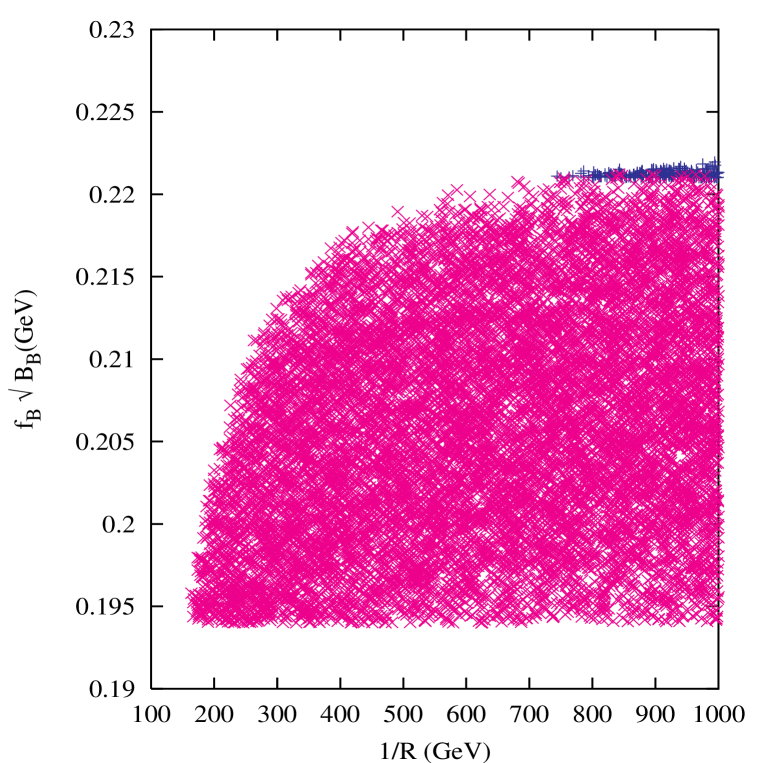
Figure 2: The region in $1/R-f_{B}\sqrt{B_{B}}$ plane allowed by the experimental value of $\Delta m_{B}$ at $1\sigma$ level with the range of the CKM parameters allowed by UUT at $1\sigma$ level. The dark region at the top corresponds to the case when the error on $f_{B}\sqrt{B_{B}}$ is reduced to one-third of its present value.

Now let us comment on possible future theoretical and experimental improvements which may modify this bound drastically. Note that the full range of the Wolfenstein parameters as mentioned in Table 1 is strongly curtailed by the allowed range of $|V_{td}|$, and it is unforeseen in near future to have such an improvement in these four parameters as to put a better constraint on $|V_{td}|$ than that coming from $B^{0}-\bar{B^{0}}$ mixing. Anyway, the bound does not change much for a marginal improvement of $|V_{td}|$. The case of $f_{B}\sqrt{B_{B}}$ is, however, different. The obtained lower bound is strongly sensitive to the value of $f_{B}\sqrt{B_{B}}$ as shown in Fig. 2. If in the future, the error in $f_{B}\sqrt{B_{B}}$ is reduced to $1/3$ of its present value, keeping the central value fixed, the lower bound on $1/R$ will be pushed up to 740 GeV. (Only the dark region in Fig. 2 will remain allowed.) If we use the CKMfitter [22] value for this quantity, viz., $230\pm 28\pm 28$ MeV, the lower bound is close to the present value, but an improvement by a factor of 3 will only push up the bound to 400 GeV.

In the case of two UEDs, the lower bound on the compactification scale (assumed same for both the dimensions) is estimated to be about $280$ GeV for $n_{s}=5$. This is fairly insensitive to the exact value of $n_{s}$ since the contributions from higher $n$ states are decoupling in nature due to GIM cancellation. This bound shots up to 1 TeV if the error bar on $f_{B}\sqrt{B_{B}}$ is again reduced threefold.

It is interesting to note that the UED contribution is always positive, increasing the value of $\Delta m_{B}$ from its SM value. Thus, if the lower bound on $f_{B}\sqrt{B_{B}}$ goes past 222 MeV, the UED models will be ruled out or at least $1/R$ will be pushed up to the multi-TeV range. The other side of the coin is that if UED has to contribute in a non-trivial way to $B^{0}-\bar{B^{0}}$ mixing, lowest-lying KK excitations are going to be detected hopefully at Tevatron run II, and definitely at the LHC.

Let us now discuss the related process $K$-${\bar{K}}$ mixing induced by box diagrams in the context of UED. This process is governed by $\Delta S=2$ effective Hamiltonian. The contribution from the KK excitations of UED is proportional to $\{\lambda_{t}^{2}[S(X_{t},X_{t})+S(X_{u},X_{u})-2S(X_{t},X_{u})]+\lambda_{c}^{2}[S(X_{c},X_{t})+S(X_{u},X_{u})-2S(X_{c},X_{u})]+\lambda_{c}\lambda_{t}[S(X_{u},X_{u})-S(X_{u},X_{t})+S(X_{c},X_{t})-S(X_{c},X_{u})]\}$. Here $|\lambda_{t}|$ (relevant for $\Delta S=2$ interactions) is suppressed by order $\lambda^{4}$ ($\lambda\simeq 0.22$ being the expansion parameter of the CKM matrix) compared to $|\lambda_{c}|$. In the context of CP violation, the term with $\lambda_{t}^{2}$ may be important as $V_{td}$ only contain the CKM phase at ${\cal O}(\lambda^{4})$. The terms proportional to $\lambda_{c}^{2}$ and $\lambda_{c}\lambda_{t}$ almost vanish as $X_{u}\simeq X_{c}\simeq{m_{n}^{2}/m_{W,n}^{2}}$. Furthermore, in $K$-${\bar{K}}$ mixing there are large long distance contributions in which the intermediate states in the transition $K\to{\bar{K}}$ are mesons instead of up type quarks and bosons. The short distance corrections are not well under control even at NLO due to the renormalisation scale ambiguity. Furthermore, there is still a large uncertainty in the determination of the bag factor $B_{K}$ for the $K$ system. Thus the study of $K$-${\bar{K}}$ mixing in the light of UED models is not promising.

To summarize, we have studied the $B^{0}-\bar{B^{0}}$ mixing in a UED model. We find lower limit for the compactification scale (165 GeV), which is close to the limits from other processes. In addition, we note that even modest theoretical improvements will have a considerable effect on the bound. With the error on $f_{B}\sqrt{B_{B}}$ reduced to one third, the bound is pushed up to 740 GeV. Thus, $B^{0}-\bar{B^{0}}$ mixing may provide us with a useful tool to discover or strictly constrain the UED models. Unfortunately, the same cannot be said for the $K$ system.

Note added. After this work was completed, a paper came to the archive [23] where the authors have discussed the same effect in the context of UED and pointed out an error in our calculation. Their results are in agreement with our corrected calculation.

Acknowledgements

The authors thank K. Agashe, A.J. Buras, M. Spranger and A. Weiler for useful discussions and comments. They also thank the organisers of WHEPP-7 in HRI, Allahabad, where this work started. DC and KH thank the Academy of Finland (project number 48787) for financial support. AK’s work has been supported by the BRNS grant 2000/37/10/BRNS of DAE, Govt. of India, the grant F.10-14/2001 (SR-I) of UGC, India, and by the fellowship of the Alexander von Humboldt Foundation.

References

• [1] K.R. Dienes, E. Dudas, T. Gherghetta, Phys. Lett. B436 (1998) 55, Nucl. Phys. B537 (1999) 47.
• [2] I. Antoniadis, Phys. Lett. B246 (1990) 377; I. Antoniadis, C. Munoz, M. Quiros, Nucl. Phys. B397 (1993) 515; I. Antoniadis, K. Benakli, Phys. Lett. B326 (1994) 69.
• [3] K.R. Dienes, E. Dudas, T. Gherghetta, Nucl. Phys. B557 (1999) 25; N. Arkani-Hamed, S. Dimopoulos, G.R. Dvali, J. March-Russell, Phys. Rev. D65 (2002) 024032.
• [4] N. Arkani-Hamed, M. Schmaltz, Phys. Rev. D61 (2000) 033005.
• [5] N. Arkani-Hamed, S. Dimopoulos, G. Dvali, Phys. Lett. B429 (1998) 263, Phys. Rev. D59 (1999) 086004.
• [6] T. Appelquist, H.-C. Cheng, B. A. Dobrescu, Phys. Rev. D64 (2001) 035002.
• [7] G. Servant, T.M.P. Tait, hep-ph/0206071, hep–ph/0209262; D. Hooper, G. D. Kribs, hep–ph/0208261; H.-C. Cheng, J. L. Feng, K. T. Matchev, Phys. Rev. Lett. 89 (2002) 211301 ; D. Majumdar, hep–ph/0209277; G. Bertone, G. Servant, G. Sigl, hep–ph/0211342.
• [8] H.-C. Cheng, K.T. Matchev, M. Schmaltz, Phys. Rev. D66 (2002) 036005.
• [9] H. Georgi, A. K. Grant, G. Hailu, Phys. Lett. B506 (2001) 207.
• [10] P. Nath, Y. Yamada, M. Yamaguchi, Phys. Lett. B466 (1999) 100; I. Antoniadis, K. Benakli, M. Quiros, Phys. Lett. B460 (1999) 176; T.G. Rizzo, J.D. Wells, Phys. Rev. D61 (200) 016007;
• [11] M. Masip, A. Pomarol, Phys. Rev. D60 (1999) 096005; C.D. Carone, Phys. Rev. D61 (2000) 015008; J. Papavassiliou, A. Santamaria, Phys. Rev. D63 (2001) 016002.
• [12] T.G. Rizzo, Phys. Rev. D64 (2001) 095010; C. Macesanu, C.D. McMullen, S. Nandi, Phys. Rev. D66 (2002) 015009; C. Macesanu, C.D. McMullen, S. Nandi, Phys. Lett. B546 (2002) 253; H.-C. Cheng, hep–ph/0206035.
• [13] K. Agashe, N.G. Deshpande, G.-H. Wu, Phys. Lett. B511 (2001) 85; T. Appelquist, B.A. Dobrescu, Phys. Lett. B516 (2001) 85;
• [14] F.J. Petriello, Jour. High Energy Phys. 0209:030 (2002); T. Appelquist, H.-U. Yee, hep–ph/0211023.
• [15] K. Agashe, N.G. Deshpande, G.-H. Wu, Phys. Lett. B514 (2001) 309.
• [16] A. van Proeyen, hep-th/9910030.
• [17] E. Gabrielli and G.F. Giudice, Nucl. Phys. B433 (1995) 3.
• [18] P.J. Franzini, Phys. Rep. 173 (1989) 1; A. Buras, Lectures given at Les Houches Summer School in Theoretical Physics, Session 68: Probing the Standard Model of Particle Interactions, Les Houches, France (1997), ed. by R. Gupta, A. Morel, E. de Rafael and F. David, North-Holland (1999).
• [19] L. Lellouch and C.J.D. Lin (UKQCD Collab.), Phys. Rev. D64 (2001) 094501; L. Lellouch, hep–ph/0211359.
• [20] A.J. Buras et al, Phys. Lett. B500 (2001) 161.
• [21] A.J. Buras, F. Parodi, A. Stocchi, hep–ph/0207101; A.J. Buras, hep–ph/0210291.
• [22] S. Laplace, hep-ph/0209188.
• [23] A.J. Buras, M. Spranger, A. Weiler, hep–ph/0212143.