Abstract

We present analytic results for first order radiative QCD corrections to $e^{+}e^{-}$ annihilation processes into quarks and gluons under the special aspect of polarized final state particles. This aspect involves single-spin polarization, gluon polarization, and the correlation between quark spins for massive final state quarks.

Invited talk given at the Füüsika Instituut,
Tartu Ülikool, Estonia, May 14th, 2002

1 Introduction

Quark mass effects play an important role in the production of quarks and gluons in $e^{+}e^{-}$ annihilations. Jet definition schemes, event shape variables, heavy flavour momentum correlations and the polarization of quarks and gluons are affected by the presence of quark masses for charm and bottom quarks even when they are produced at the scale of the $Z^{0}$ mass [1, 2, 3]. A careful investigation of quark mass effects in $e^{+}e^{-}$ annihilations may even lead to an alternative determination of the quark mass values [1, 2, 3, 4].

There is an obvious interest in quark mass effects for $t\bar{t}$ production where quark mass effects cannot be neglected in the envisaged range of energies to be covered by the Next Linear Collider (NLC). The longitudinal polarization of massive quarks affects the shape of the energy spectrum of their secondary decay leptons, the longitudinal spin-spin correlation effects in pair produced quarks and antiquarks will lead to correlation effects of the energy spectra of their secondary decay leptons and antileptons. Quark mass effects are important in the $m\to 0$ calculation of radiative corrections to quark polarization variables because residual mass effects change the naive no-flip pattern of the $m=0$ polarization results [5, 6].

In this talk I present $O(\alpha_{s})$ radiative corrections to different polarization observables, namely the longitudinal and transverse single-spin polarization of the quark [7, 8, 9, 10], the polarization of the gluon [11, 12], and the longitudinal spin-spin correlation [13, 14] for massive quark pairs produced in $e^{+}e^{-}$ annihilations, always including the polar angle dependence. As a byproduct of our calculations I discuss the $m\to 0$ limit and the role of the $O(\alpha_{s})$ residual mass effects. I explain how residual mass effects contribute to the various spin-flip and no-flip terms in the $m\to 0$ limit for each of the three structure functions that describe the polar angle dependence.

2 The joint quark-antiquark density matrix

Let us start with the joint quark-antiquark density matrix $d\hbox{$\kern 2.5pt\vrule height=4.0pt\kern-2.5pt\sigma$}^{\alpha}=d\sigma^{\alpha}_{\lambda_{1}\lambda_{2};\lambda^{\prime}_{1}\lambda^{\prime}_{2}}$ where $\lambda_{1}$ and $\lambda_{2}$ denote the helicities of the quark and antiquark, respectively. In the applications covered by this talk, only the diagonal case $\lambda_{1}=\lambda^{\prime}_{1}$ and $\lambda_{2}=\lambda^{\prime}_{2}$ is of importance. The label $\alpha$ specifies the polarization of the initial $\gamma^{*}$, $Z$ or interference contributions thereof. This index will be specified later on by the labels $U$ (unpolarized transverse), $L$ (longitudinal), $F$ (forward–backward), and the two labels $A$ and $I$ for the case of transverse polarization of the final state quarks.

The diagonal part of the differential joint density matrix can be represented in terms of its components along the products of the unit matrix and the $z$-components of the Pauli matrix $\hbox{$\kern 2.5pt\vrule height=4.0pt\kern-2.5pt\sigma$}_{3}$ ($\hbox{$\kern 2.5pt\vrule height=4.0pt\kern-2.5pt\sigma$}_{3}=\hat{p}_{1}\vec{\hbox{$\kern 2.5pt\vrule height=4.0pt\kern-2.5pt\sigma$}}$ for the quark and $\hbox{$\kern 2.5pt\vrule height=4.0pt\kern-2.5pt\sigma$}_{3}=\hat{p}_{2}\vec{\hbox{$\kern 2.5pt\vrule height=4.0pt\kern-2.5pt\sigma$}}$ for the antiquark, $\hat{p}_{i}=\vec{p}_{i}/|\vec{p}_{i}|$). One has

$$d\hbox{$\kern 2.5pt\vrule height=4.0pt\kern-2.5pt\sigma$}^{\alpha}=\frac{1}{4}\left(d\sigma_{\alpha}\hbox{$1\kern-2.5pt\hbox{\rm l}$}\otimes\hbox{$1\kern-2.5pt\hbox{\rm l}$}+d\sigma_{\alpha}^{(\ell_{1})}\hbox{$\kern 2.5pt\vrule height=4.0pt\kern-2.5pt\sigma$}_{3}\otimes\hbox{$1\kern-2.5pt\hbox{\rm l}$}+d\sigma_{\alpha}^{(\ell_{2})}\hbox{$1\kern-2.5pt\hbox{\rm l}$}\otimes\hbox{$\kern 2.5pt\vrule height=4.0pt\kern-2.5pt\sigma$}_{3}+d\sigma_{\alpha}^{(\ell_{1}\ell_{2})}\hbox{$\kern 2.5pt\vrule height=4.0pt\kern-2.5pt\sigma$}_{3}\otimes\hbox{$\kern 2.5pt\vrule height=4.0pt\kern-2.5pt\sigma$}_{3}\right)$$ (1)

as formulated for longitudinal polarization, the first and the second Pauli matrices stand for the quark and the antiquark, respectively. An alternative but equivalent representation of the longitudinal spin contributions can be written down in terms of the longitudinal spin components $s_{1}^{\ell}=2\lambda_{1}$ and $s_{2}^{\ell}=2\lambda_{2}$ with $s_{1}^{\ell},s_{2}^{\ell}=\pm 1$ (or $s_{1}^{\ell},s_{2}^{\ell}\in\{\uparrow,\downarrow\}$). The spin dependent parts of the differential cross section are given by

$$d\sigma_{\alpha}(s_{1}^{\ell},s_{2}^{\ell})=\frac{1}{4}\left(d\sigma_{\alpha}+d\sigma^{(\ell_{1})}_{\alpha}s_{1}^{\ell}+d\sigma^{(\ell_{2})}_{\alpha}s_{2}^{\ell}+d\sigma^{(\ell_{1}\ell_{2})}_{\alpha}s_{1}^{\ell}s_{2}^{\ell}\right).$$ (2)

Eq. (2) is easily inverted,

$$d\sigma_{\alpha} = d\sigma_{\alpha}(\uparrow\uparrow)+d\sigma_{\alpha}(\uparrow\downarrow)+d\sigma_{\alpha}(\downarrow\uparrow)+d\sigma_{\alpha}(\downarrow\downarrow),$$

$$d\sigma_{\alpha}^{(\ell_{1})} = d\sigma_{\alpha}(\uparrow\uparrow)+d\sigma_{\alpha}(\uparrow\downarrow)-d\sigma_{\alpha}(\downarrow\uparrow)-d\sigma_{\alpha}(\downarrow\downarrow),$$

$$d\sigma_{\alpha}^{(\ell_{2})} = d\sigma_{\alpha}(\uparrow\uparrow)-d\sigma_{\alpha}(\uparrow\downarrow)+d\sigma_{\alpha}(\downarrow\uparrow)-d\sigma_{\alpha}(\downarrow\downarrow),$$

$$d\sigma_{\alpha}^{(\ell_{1}\ell_{2})} = d\sigma_{\alpha}(\uparrow\uparrow)-d\sigma_{\alpha}(\uparrow\downarrow)-d\sigma_{\alpha}(\downarrow\uparrow)+d\sigma_{\alpha}(\downarrow\downarrow).$$ (3)

The first line is the unpolarized contribution, the second line the contribution due to a single polarized quark, while the last line is the correlation between quark and antiquark. While all these contributions will be considered in the following, the polarisation of a single antiquark (third line) is not considered because it is equivalent to the case of a single polarized quark.

2.1 The differential cross section

According to Fermi’s “golden rule” the differential cross section is given by

$$d\sigma=2\pi|T_{fi}|^{2}dPS.$$ (4)

Using conventional Feynman rules, especially

$$-ieQ_{f}\gamma_{\mu}\quad\mbox{and}\quad-ie(v_{f}\gamma_{\mu}-a_{f}\gamma_{\mu}\gamma_{5})$$ (5)

for the vertex of the fermion line with a photon or a $Z$ boson, respectively, and

$$\frac{-ig^{\mu\nu}}{q^{2}}\quad\mbox{and}\quad\chi_{Z}(q)\frac{-ig^{\mu\nu}}{q^{2}}$$ (6)

for the boson propagators with momentum $q$, one can write

$$T_{fi}\ =\ \bar{v}(p_{2})\Big{[}-ieQ_{f}\gamma^{\mu}\Big{]}u(p_{1})\frac{-i}{q^{2}}\bar{v}(p_{+})\Big{[}-ieQ_{e}\gamma_{\mu}\Big{]}u(p_{-})\,+$$ (7)

$$+\bar{v}(p_{2})\Big{[}-ie(v_{f}\gamma^{\mu}-a_{f}\gamma^{\mu}\gamma_{5})\Big{]}u(p_{1})\chi_{Z}(q)\frac{-i}{q^{2}}\bar{v}(p_{+})\Big{[}-ie(v_{e}\gamma_{\mu}-a_{e}\gamma_{\mu}\gamma_{5})\Big{]}u(p_{-})\qquad$$

where $p_{-}$ and $p_{-}$ are the moments of the electron and positron, $p_{1}$ and $p_{2}$ are the moments of the quark and antiquark, and $q=p_{-}+p_{+}=p_{1}+p_{2}$ is the moment of the boson. Possible polarisation degrees of freedom enter the squared matrix element by replacing for instance $u(p_{1})\bar{u}(p_{1})$ by $(\gamma_{\mu}p_{1}^{\mu}+m)(1+\gamma_{5}\gamma_{\nu}s_{1}^{\nu})/2$ instead of summing over the polarisations of the final state. $m$ is the mass of the quark (and antiquark). The squared matrix element reads

$$|T_{fi}|^{2}=g_{ij}L_{\mu\nu}^{i}H^{j\mu\nu}$$ (8)

where $L_{\mu\nu}^{i}$ contains all elements due to electron and positron (lepton tensor), $H^{j\mu\nu}$ contains all elements due to the quark and antiquark (hadron tensor), and $g_{ij}$ contains the elements due to the intemediate bosons (photon and $Z$ boson) which mix up. These parts will be considered in turn.

2.2 The hadron tensor

The hadron tensor is determined by the hadron dynamics, i.e. by the current-induced production of a quark-antiquark pair which, in the $O(\alpha_{s})$ case, is followed by gluon emission. In the $O(\alpha_{s})$ case one also has to add the one-loop contribution. The index $i=1,2,3,4$ in Eq. (8) specifies the current composition in terms of the parity-even (for $i=1,2$) and parity-odd ($i=3,4$) products of the vector and the axial vector currents according to

$$H^{1}_{\mu\nu}=\frac{1}{2}(H^{VV}_{\mu\nu}+H^{AA}_{\mu\nu}), H^{2}_{\mu\nu}=\frac{1}{2}(H^{VV}_{\mu\nu}-H^{AA}_{\mu\nu}),$$

$$H^{3}_{\mu\nu}=\frac{i}{2}(H^{VA}_{\mu\nu}-H^{A\,V}_{\mu\nu}), H^{4}_{\mu\nu}=\frac{1}{2}(H^{VA}_{\mu\nu}+H^{A\,V}_{\mu\nu}).$$ (9)

In order to be specific, the unpolarized hadron tensor $H_{\mu\nu}^{VA}$ is e.g. given by the matrix element

$$H_{\mu\nu}^{VA}=\langle q\bar{q}|J_{\mu}^{V}|0\rangle\langle 0|(J_{\nu}^{A})^{\dagger}|q\bar{q}\rangle.$$ (10)

In the two-body case $e^{+}e^{-}\to q\bar{q}$ the components of the cross section are given by

$$\sigma_{\alpha}^{i(P)}=\frac{\pi\alpha^{2}v}{3q^{4}}H_{\alpha}^{i(P)}\qquad\left(\mbox{with\ }v=\sqrt{1-4m^{2}/q^{2}}\right)$$ (11)

where $(P)$ stands for unpolarized, single-spin or spin-spin correlation contributions. In the three-body case $e^{+}e^{-}\to q\bar{q}g$ the hadron tensor components $H_{\alpha}^{i(P)}(y,z)$ are related to the components of the differential cross section by

$$\frac{d\sigma_{\alpha}^{i(P)}}{dy\,dz}=\frac{\pi\alpha^{2}v}{3q^{4}}\left\{\frac{q^{2}}{16\pi^{2}v}H_{\alpha}^{i(P)}(y,z)\right\}.$$ (12)

The two energy-type variables $y=1-2p_{1}q/q^{2}$ and $z=1-2p_{2}q/q^{2}$ are used as kinematic variables. Note that the three-body helicity structure functions $H_{\alpha}^{i(P)}(y,z)$ have a different dimension than their two-body counterparts in Eq. (12) which we indicate by explicitly referring to the $(y,z)$-dependence of the three-body structure functions. An example for the phase space in terms of $y$ and $z$ is shown in Fig. 4.

2.3 The electro-weak form factors

The second building block $g_{ij}$ ($i,j=1,2,3,4$) specifies the electro-weak model dependence of the $e^{+}e^{-}$ cross section. For the present discussion we need the components $g_{11}$, $g_{12}$, $g_{43}$ and $g_{44}$. They are given by

$$g_{11} = Q_{f}^{2}-2Q_{f}v_{e}v_{f}\mathop{\rm Re}\nolimits\chi_{Z}+(v_{e}^{2}+a_{e}^{2})(v_{f}^{2}+a_{f}^{2})|\chi_{Z}|^{2},$$

$$g_{12} = Q_{f}^{2}-2Q_{f}v_{e}v_{f}\mathop{\rm Re}\nolimits\chi_{Z}+(v_{e}^{2}+a_{e}^{2})(v_{f}^{2}-a_{f}^{2})|\chi_{Z}|^{2},$$

$$g_{13} = -2Q_{f}v_{e}a_{f}\mathop{\rm Im}\nolimits\chi_{Z},$$

$$g_{14} = 2Q_{f}v_{e}a_{f}\mathop{\rm Re}\nolimits\chi_{Z}-2(v_{e}^{2}+a_{e}^{2})v_{f}a_{f}|\chi_{Z}|^{2},$$ (13)

$$g_{21} = q_{f}^{2}-2Q_{f}v_{e}v_{f}\mathop{\rm Re}\nolimits\chi_{Z}+(v_{e}^{2}-a_{e}^{2})(v_{f}^{2}+a_{f}^{2})|\chi_{Z}|^{2},$$

$$g_{22} = q_{f}^{2}-2Q_{f}v_{e}v_{f}\mathop{\rm Re}\nolimits\chi_{Z}+(v_{e}^{2}-a_{e}^{2})(v_{f}^{2}-a_{f}^{2})|\chi_{Z}|^{2},$$

$$g_{23} = -2Q_{f}v_{e}a_{f}\mathop{\rm Im}\nolimits\chi_{Z},$$

$$g_{24} = 2Q_{f}v_{e}a_{f}\mathop{\rm Re}\nolimits\chi_{Z}-2(v_{e}^{2}-a_{e}^{2})v_{f}a_{f}|\chi_{Z}|^{2},$$ (14)

$$g_{31} = -2Q_{f}a_{e}v_{f}\mathop{\rm Im}\nolimits\chi_{Z},$$

$$g_{32} = -2Q_{f}a_{e}v_{f}\mathop{\rm Im}\nolimits\chi_{Z},$$

$$g_{33} = 2Q_{f}a_{e}a_{f}\mathop{\rm Re}\nolimits\chi_{Z},$$

$$g_{34} = 2Q_{f}a_{e}a_{f}\mathop{\rm Im}\nolimits\chi_{Z},$$ (15)

$$g_{41} = 2Q_{f}a_{e}v_{f}\mathop{\rm Re}\nolimits\chi_{Z}-2v_{e}a_{e}(v_{f}^{2}+a_{f}^{2})|\chi_{Z}|^{2},$$

$$g_{42} = 2Q_{f}a_{e}v_{f}\mathop{\rm Re}\nolimits\chi_{Z}-2v_{e}a_{e}(v_{f}^{2}-a_{f}^{2})|\chi_{Z}|^{2},$$

$$g_{43} = 2Q_{f}a_{e}a_{f}\mathop{\rm Im}\nolimits\chi_{Z},$$

$$g_{44} = -2Q_{f}a_{e}a_{f}\mathop{\rm Re}\nolimits\chi_{Z}+4v_{e}a_{e}v_{f}a_{f}|\chi_{Z}|^{2}$$ (16)

where $\chi_{Z}(q^{2})=gM_{Z}^{2}q^{2}/(q^{2}-M_{Z}^{2}+iM_{Z}\Gamma_{Z})$, with $M_{Z}$ and $\Gamma_{Z}$ the mass and width of the $Z^{0}$ ($M_{Z}=91.1887{\rm\,GeV}$ and $\Gamma_{Z}=2.487{\rm\,GeV}$ [15]) and $g=G_{F}(8\sqrt{2}\pi\alpha)^{-1}\approx 4.49\times 10^{-5}\mbox{\rm GeV}^{-2}$. $Q_{f}$ are the charges of the final state quarks to which the electro-weak currents directly couple; $v_{e}$ and $a_{e}$, $v_{f}$ and $a_{f}$ are the electro-weak vector and axial vector coupling constants. For example, in the Weinberg–Salam model, one has $v_{e}=-1+4\sin^{2}\theta_{W}$, $a_{e}=-1$ for leptons, $v_{f}=1-\frac{8}{3}\sin^{2}\theta_{W}$, $a_{f}=1$ for up-type quarks ($Q_{f}=\frac{2}{3}$), and $v_{f}=-1+\frac{4}{3}\sin^{2}\theta_{W}$, $a_{f}=-1$ for down-type quarks ($Q_{f}=-\frac{1}{3}$). The left- and right-handed coupling constants are then given by $g_{L}=v+a$ and $g_{R}=v-a$, respectively. In the purely electromagnetic case one has $g_{11}=g_{12}=g_{21}=g_{22}=Q_{f}^{2}$ and all other $g_{r^{\prime}r}=0$. The terms linear in $\mathop{\rm Re}\nolimits\chi_{Z}$ and $\mathop{\rm Im}\nolimits\chi_{Z}$ come from $\gamma-Z^{0}$ interference, whereas the terms proportional to $|\chi_{Z}|^{2}$ originate from $Z$-exchange.

The generalization of the case where one starts with longitudinally polarized beams is straightforward and amounts to the replacement

$$g_{1i}\rightarrow(1-h^{-}h^{+})g_{1i}+(h^{-}-h^{+})g_{4i}\qquad g_{4i}\rightarrow(1-h^{-}h^{+})g_{4i}+(h^{-}-h^{+})g_{1i}$$ (17)

where $h^{-}$ and $h^{+}$ ($-1\leq h^{\pm}\leq+1$) denote the longitudinal polarization of the electron and the positron beam, respectively. Clearly there is no interaction between the beams when $h^{+}=h^{-}=\pm 1$.

2.4 The polar angle dependence

As mentioned in the introduction, the polar angle dependence will be determined. The rest frame of the boson is a natural choice for the considerations. However, two coordinate systems are in use here, the event frame for the outgoing particles and the beam frame for the incoming particles. Transforming from one to the other system brings in a relative polar angle $\theta$ (and in case of transverse spin vectors also a azimuthal angle $\varphi$ which is averaged out normally). The polar angle $\theta$ is given by the angle between the colliding electron beam direction and the outgoing quark direction. Transformed to the event frame, the lepton tensor $L_{\mu\nu}^{i}$ leads to the different angular distributions. While for massless leptons the components $L_{\mu\nu}^{2}$ and $L_{\mu\nu}^{3}$ vanish, one can decompose the remaining lepton tensor components according to

$$L^{1} = \frac{q^{2}}{2}\left\{\frac{1}{2}(1+\cos^{2}\theta){\mit\Pi}_{U}+\sin^{2}\theta\,{\mit\Pi}_{L}+\sin\theta\cos\theta\,{\mit\Pi}_{I}\right\},$$

$$L^{4} = \frac{q^{2}}{2}\left\{\cos\theta\,{\mit\Pi}_{F}+\sin\theta\,{\mit\Pi}_{A}\right\}.$$ (18)

Remark that ${\mit\Pi}_{I}$ and ${\mit\Pi}_{A}$ depend linearly on $\sin\varphi$ and $\cos\varphi$. The matrices ${\mit\Pi}_{U}$, ${\mit\Pi}_{L}$, ${\mit\Pi}_{I}$, ${\mit\Pi}_{F}$ and ${\mit\Pi}_{A}$ are called projectors because in contracting the lepton tensor with the hadron tensor they project out the contribution of the hadron tensor to the different angle dependences. Explicit projectors are

$${\mit\Pi}_{U}^{\mu\nu} = -\hat{g}^{\mu\nu}-\frac{\hat{p}_{1}^{\mu}\hat{p}_{1}^{\nu}}{p_{1z}^{2}},\qquad{\mit\Pi}_{L}^{\mu\nu}\ =\ \frac{\hat{p}_{1}^{\mu}\hat{p}_{1}^{\nu}}{p_{1z}^{2}},\qquad{\mit\Pi}_{F}^{\mu\nu}\ =\ i\varepsilon^{\mu\nu\alpha\beta}\frac{\hat{p}_{1\alpha}q_{\beta}}{p_{1z}\sqrt{q^{2}}},$$ (19)

$${\mit\Pi}_{I}^{\mu\nu} = s_{1}^{\mu}\hat{p}_{1}^{\nu}+\hat{p}_{1}^{\mu}s_{1}^{\nu},\qquad{\mit\Pi}_{A}^{\mu\nu}\ =\ i\varepsilon^{\mu\nu\alpha\beta}q_{\alpha}s_{1\beta}\qquad(\hat{g}^{\mu\nu}=g^{\mu\nu}-q^{\mu}q^{\nu}/q^{2},\ \hat{p}_{i}=\vec{p}_{i}/|\vec{p}_{i}|)$$

The decomposition in Eq. (2.4) covers all possible angle dependences which occur in the process with a single polarized quark. This decomposition gives rise to the decomposition of the differential cross section according to

$$\frac{d\sigma^{(P)}}{d\cos\theta} = \frac{3}{8}(1+\cos^{2}\theta)\sigma_{U}^{(P)}+\frac{3}{4}\sin^{2}\theta\sigma_{L}^{(P)}+\frac{3}{4}\cos\theta\sigma_{F}^{(P)}\,+$$ (20)

$$\qquad+\frac{3}{4}\sin\theta\cos\theta\sigma_{I}^{(P)}+\frac{3}{4}\sin\theta\sigma_{A}^{(P)}$$

3 Unpolarized and polarized structure functions

In Ref. [7] the mean longitudinal polarization of the quark (i.e. the average over the polar angle $\theta$) was calculated, while in Refs. [8, 10] the polar angle dependence was determined, including beam polarisation effects. The polar angle dependence of the transverse polarisation was considered in Ref. [9]. In this section I present the results and show a few instructive steps of the calculations.

Figure 1: Born term contributions to the single spin case

3.1 Born term contributions

The Born term contributions are easy to calculate. The Feynman diagrams for the hadronic part (in case of the single polarized case) are shown in Fig. 1. The unpolarized contributions are given by

$$H_{U}^{1}({\it born\/})=2N_{c}q^{2}(1+v^{2}), H_{L}^{1}({\it born\/})=N_{c}q^{2}(1-v^{2})\ =\ H_{L}^{2}({\it born\/}),$$

$$H_{U}^{2}({\it born\/})=2N_{c}q^{2}(1-v^{2}), H_{F}^{4}({\it born\/})=4N_{c}q^{2}v.$$ (21)

where $N_{c}$ is the number of colours. The longitudinally polarized contributions read

$$H_{U}^{4\ell}({\it born\/})=4N_{c}q^{2}v, H_{F}^{1\ell}({\it born\/})=2N_{c}q^{2}(1+v^{2}),$$

$$H_{L}^{4\ell}({\it born\/})=0, H_{F}^{2\ell}({\it born\/})=2N_{c}q^{2}(1-v^{2}).$$ (22)

For the transverse polarization we finally obtain

$$H_{I}^{4\perp}({\it born\/})=-2N_{c}q^{2}v\sqrt{\xi}, H_{A}^{1\perp}({\it born\/})=-2N_{c}q^{2}\sqrt{\xi}=H_{A}^{2\perp}({\it born\/}),$$ (23)

$$H_{A}^{3N}({\it born\/})=2N_{c}q^{2}\sqrt{\xi}$$

where $\xi=4m^{2}/q^{2}=1-v^{2}$ and “$\perp$” and “$N$” indicate the transverse polarisations perpendicular and normal to the event plane.

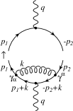
Figure 2: Loop contributions to the single spin case

3.2 First order loop contributions

The calculation of loop contributions can be formally be done by using the vertex form factors, i.e. by replacing the vector and axial vector vertices according to

$$\gamma^{\mu}\rightarrow(1+A)\gamma^{\mu}+B(p_{1}-p_{2})^{\mu},\qquad\gamma^{\mu}\gamma_{5}\rightarrow\left((1+C)\gamma^{\mu}+D(p_{1}+p_{2})^{\mu}\right)\gamma_{5}.$$ (24)

The squared matrix element including first order loop corrections contains the Born term contributions as well as first and second order contributions. Only the first order contributions, as shown in Fig. 2, are used for a first order calculation. The non-vanishing contributions read

$$H_{U}^{1}({\it loop\/}) = 4N_{c}q^{2}\left((1+v^{2})\mathop{\rm Re}\nolimits A-2v^{2}\mathop{\rm Re}\nolimits B\right),$$

$$H_{U}^{2}({\it loop\/}) = 4N_{c}q^{2}\left((1-v^{2})\mathop{\rm Re}\nolimits A+2v^{2}\mathop{\rm Re}\nolimits B\right),$$

$$H_{L}^{1}({\it loop\/}) = 2N_{c}q^{2}\left((1-v^{2})\mathop{\rm Re}\nolimits A+v^{2}\mathop{\rm Re}\nolimits B\right)\ =\ H_{L}^{2}({\it loop\/}),$$

$$H_{F}^{4}({\it loop\/}) = 8N_{c}q^{2}v\left(\mathop{\rm Re}\nolimits A-\mathop{\rm Re}\nolimits B\right),$$

$$H_{U}^{4\ell}({\it loop\/}) = 8N_{c}q^{2}v\left(\mathop{\rm Re}\nolimits A-\mathop{\rm Re}\nolimits B\right),\qquad H_{L}^{4\ell}({\it loop\/})\ =\ 0,$$

$$H_{F}^{1\ell}({\it loop\/}) = 4N_{c}q^{2}\left((1+v^{2})\mathop{\rm Re}\nolimits A-2v^{2}\mathop{\rm Re}\nolimits B\right),$$

$$H_{F}^{2\ell}({\it loop\/}) = 4N_{c}q^{2}\left((1-v^{2})\mathop{\rm Re}\nolimits A+2v^{2}\mathop{\rm Re}\nolimits B\right),$$

$$H_{I}^{3\perp}({\it loop\/}) = -2N_{c}q^{2}v\sqrt{\xi}(1+\xi)\mathop{\rm Im}\nolimits B/\xi,$$

$$H_{I}^{4\perp}({\it loop\/}) = -2N_{c}q^{2}v\sqrt{\xi}\left(2\mathop{\rm Re}\nolimits A+(1-3\xi)\mathop{\rm Re}\nolimits B/\xi\right),$$

$$H_{A}^{1\perp}({\it loop\/}) = -2N_{c}q^{2}\sqrt{\xi}\left(\mathop{\rm Re}\nolimits A-v^{2}\mathop{\rm Re}\nolimits B/\xi\right)\ =\ H_{A}^{2\perp}({\it loop\/}),$$

$$H_{I}^{1N}({\it loop\/}) = -2N_{c}q^{2}v\sqrt{\xi}(1-\xi)\mathop{\rm Im}\nolimits B/\xi\ =\ H_{I}^{2N}({\it loop\/}),$$

$$H_{A}^{3N}({\it loop\/}) = 2N_{c}q^{2}v\sqrt{\xi}\left(2\mathop{\rm Re}\nolimits A+(1-3\xi)\mathop{\rm Re}\nolimits B/\xi\right),$$

$$H_{A}^{4N}({\it loop\/}) = 2N_{c}q^{2}v\sqrt{\xi}(1+\xi)\mathop{\rm Im}\nolimits B/\xi,$$ (25)

the vertex form factors $A$ and $B$ are given by

$$\mathop{\rm Re}\nolimits A = -\frac{\alpha_{s}C_{F}}{4\pi}\Bigg{\{}\left(2+\frac{1+v^{2}}{v}\ln\left(\frac{1-v}{1+v}\right)\right)\ln\left(\frac{\Lambda q^{2}}{m^{2}}\right)+3v\ln\left(\frac{1-v}{1+v}\right)+4$$

$$\qquad+\frac{1+v^{2}}{v}\left({\rm Li}_{2}\left(\frac{2v}{1+v}\right)+\frac{1}{4}\ln^{2}\left(\frac{1-v}{1+v}\right)-\frac{\pi^{2}}{2}\right)\Bigg{\}},$$

$$\mathop{\rm Re}\nolimits B = \frac{\alpha_{s}C_{F}}{4\pi}\ \frac{1-v^{2}}{v}\ln\left(\frac{1-v}{1+v}\right),\qquad\mathop{\rm Im}\nolimits B\ =\ \frac{\alpha_{s}C_{F}}{4\pi}\ \frac{1-v^{2}}{v}\pi$$ (26)

were we already have replaced the axial-vector form factor $C$ by $A$ according to $C=A-2B$, and where $m_{G}^{2}=\Lambda q^{2}$ is the squared mass of the gluon which we use for the regularization of the first order tree contributions and which is replaces the parameter $\varepsilon=(4-D)/2$ of the dimensional regularization by means of $1/\varepsilon-\gamma_{E}+\ln(4\pi\mu^{2}/m^{2})\rightarrow\ln(\Lambda q^{2}/m^{2})$.

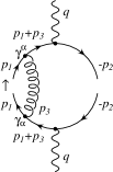
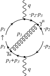
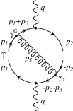
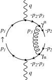
Figure 3: tree graph contributions to the single spin case

3.3 First order tree graph contributions

Even though ending up with a different final state, namely a three particle state including quark, antiquark and gluon, the first order tree graph contributions are needed for a full first order result. For vanishing gluon momentum the (soft) gluon cannot be resolved by the detector, the event is counted as two particle final state. In this soft region the infrared singularity of the three graph contribution cancels the infrared singularity of the loop contribution. This is a general result formulated in the Lee–Nauenberg theorem [5].

The hadronic part of the diagrams is shown in Fig. 3. The additional degree of freedom given by the gluon leads to two additional integration measures, expressible in the energy type variables $y$ and $z$ mentioned earlier. The three particle phase space for some specified center-of-mass energy $\sqrt{q^{2}}$ is shown in Fig. 4.

Figure 4: Example for the phase space for the three particle decay

Integrals to be calculated are of the general type ($p$ and $q$ take integer values in a finite range around zero)

$$I(\xi,\Lambda)=\int y^{p}z^{q}dy\,dz$$ (27)

where the integration limits are given by the phase space boundary,

$$y_{-} = \sqrt{\Lambda\xi}+\Lambda,\qquad y_{+}\ =\ 1-\sqrt{\xi}$$ (28)

$$z_{\pm}(y) = \frac{2y}{4y+\xi}\left\{1-y-\frac{1}{2}\xi+\Lambda+\frac{\Lambda}{y}\pm\frac{1}{y}\sqrt{(y-\Lambda)^{2}-\Lambda\xi}\sqrt{(1-y)^{2}-\xi}\right\}$$ (29)

where $\sqrt{\Lambda q^{2}}$ is again the gluon mass. While the integration over $z$ can be performed easily, the second integration is not so easy to perform, the most complicated (logarithmic) integrals are of the shape

$$I^{\prime}(\xi,\Lambda)=\int_{\sqrt{\Lambda\xi}}^{1-\sqrt{\xi}}y^{n}\ln\left(\frac{z_{+}(y)}{z_{-}(y)}\right)dy.$$ (30)

Two issues should be mentioned here. First, the gluon mass is necessary only for regularizing the integrals. Therefore, the parameter $\Lambda$ need to appear only at places where the integral at the lower limit would lead to singular expressions if the parameter were absent. A lot of integrals, therefore, can be calculated for $\Lambda=0$. On the other hand, the singular integrals can be calculated by subtracting and adding a (simpler) integral which has the same singular structure. According to

$$I^{\prime}(\xi,\Lambda)=\left(I^{\prime}(\xi,\Lambda)-I^{\prime}_{0}(\xi,\Lambda)\right)+I^{\prime}_{0}(\xi,\Lambda)=\Delta I^{\prime}(\xi,\Lambda)+I^{\prime}_{0}(\xi,\Lambda),$$ (31)

for the difference term $\Lambda=0$ can be chosen. The integral $I^{\prime}_{0}$ can be obtained from $I^{\prime}$ by taking approximations for the integrand close to the lower (infrared singular) limit, $y=\sqrt{\Lambda\xi}+\Lambda$. So

$$z_{\pm}\rightarrow\frac{1}{\xi}\left((2-\xi)y\pm 2\sqrt{(y-\Lambda)^{2}-\Lambda\xi}\sqrt{1-\xi}\right)$$ (32)

and a substitution $y=\Lambda+\sqrt{\Lambda\xi}\cosh\zeta$ helps for the integration. For the integrals with $\Lambda=0$, on the other hand, a combined substitution $y=1-\sqrt{\xi}(1+z^{2})/(1-z^{2})$ works to separate the integral into integrable pieces. The results can be finally expressed in a very compact form by using the so-called decay rate terms. At this point I only show the results for the unpolarized case for reasons of brevity, the spin-dependent parts are only different but not more complicated, ($N=\alpha_{s}N_{c}C_{f}/4\pi v$)

$$H_{U}^{1}(\alpha_{s}) = N\Big{\{}2(2+7\xi)v+(48-48\xi+7\xi^{2})t_{3}+2\sqrt{\xi}\left(2-7\xi+\sqrt{\xi}(2+3\xi)\right)t_{4}$$

$$-2\xi(2+3\xi)t_{5}-4(2-\xi)\left((2-\xi)(t_{8}-t_{9})+2v(t_{10}+2t_{12})\right)\Big{\}},$$

$$H_{U}^{2}(\alpha_{s}) = \xi N\Big{\{}12v+2(6-\xi)t_{3}+2\sqrt{\xi}(1-\sqrt{\xi})t_{4}$$

$$+2\xi t_{5}-4\left((2-\xi)(t_{8}-t_{9})+2v(t_{10}+2t_{12})\right)\Big{\}},$$

$$H_{L}^{1}(\alpha_{s}) = \!\!N\Big{\{}\frac{1}{2}(16-46\xi+3\xi^{2})v+\frac{\xi}{4}(88-32\xi+3\xi^{2})t_{3}$$

$$-2\sqrt{\xi}\left(2-7\xi+\sqrt{\xi}(2+3\xi)\right)t_{4}+2\xi(2+3\xi)t_{5}$$

$$-2\xi\left((2-\xi)(t_{8}-t_{9})+2v(t_{10}+2t_{12})\right)\Big{\}},$$

$$H_{L}^{2}(\alpha_{s}) = \xi N\Big{\{}\frac{3}{2}(10-\xi)v+\frac{1}{4}(24-16\xi-3\xi^{2})t_{3}$$

$$-2\sqrt{\xi}(1-\sqrt{\xi})t_{4}-2\xi t_{5}-2\left((2-\xi)(t_{8}-t_{9})+2v(t_{10}+2t_{12})\right)\Big{\}},$$

$$H_{F}^{3}(\alpha_{s}) = -8\xi Nv\pi,$$

$$H_{F}^{4}(\alpha_{s}) = N\Big{\{}-16\sqrt{\xi}(1-\sqrt{\xi})-16(t_{1}-t_{2})+8(2-3\xi)vt_{3}$$ (33)

$$-4(4-5\xi)t_{6}-8v\left((2-\xi)(t_{8}-t_{7})+2v(t_{10}+t_{11})\right)\Big{\}}$$

where the decay rate terms, containing logarithms and dilogarithms, are found in Ref. [10] together with the polarized contributions. More interesting at this point are the results we obtain. In Fig. 6 (top) the total cross section for pair production of top quarks is shown in dependence on the center-of-mass energy $\sqrt{q^{2}}$, with and without the first order radiative correction. The polar angle dependence of the longitudinal polarization

$$P=\frac{d\sigma(\uparrow)-d\sigma(\downarrow)}{d\sigma(\uparrow)+d\sigma(\downarrow)}$$ (34)

of the top quark is shown in Fig. 6 (bottom). In Fig. 7 the polar angle dependence of the normal (top) and perpendicular polarization (bottom) of the top quark is displayed. What is not shown here is the change with respect to the Born term contribution. It figures out that despite the fact of rather large corrections to the total cross section, the corrections to the polarizations are quite small (about 5%). A detailed discussion of the results can be found in Refs. [8, 9, 10]. Quantities like the polarization can be measured by the asymmetry of the decay products of the top quark.

3.4 Finite gluon energy cut

Besides the comparison with the massless case, resulting in anomalous spin-flip contributions which will be shown later, additional work has been investigated in the exact calculation of the contributions for a given gluon energy cut, dividing the phasespace up into a soft and a hard part [16]. This “excurse” will not be taken here.

4 Longitudinal spin correlation

If both quark and antiquark are considered to be polarized, the correlation between their spins can be measured. In Ref. [13] the correlation of longitudinal polarized quark and antiquark is considered, in Ref. [14] the angular dependence is considered as well. Because of the representation

$$(s_{1}^{\ell})^{\mu} = \frac{s_{1}^{\ell}}{\sqrt{\xi}}(\sqrt{(1-y)^{2}-\xi};0,0,1-y)$$ (35)

$$(s_{2}^{\ell})^{\mu} = \frac{s_{2}^{\ell}}{\sqrt{\xi}}(\sqrt{(1-z)^{2}-\xi};(1-z)\sin\theta_{12},0,(1-z)\cos\theta_{12})$$

for the longitudinal spins where

$$\cos\theta_{12}=\frac{yz+y+z-1+\xi}{\sqrt{(1-y)^{2}-\xi}\sqrt{(1-z)^{2}-\xi}},$$ (36)

there occurs an additional square root $\sqrt{(1-z)^{2}-\xi}$ in the denominator which makes the integrations more complicated. However, the same integration methods work also in this case, an appropiate substitution could be found to make the integration feasible. New decay rate terms had to be defined in order to describe the final result (see Ref. [14]).

Figure 5: Correlation of longitudinal top and antitop spin

4.1 Result for the correlation

The correlation is defined as

$$C=\frac{d\sigma(\uparrow\uparrow)-d\sigma(\uparrow\downarrow)-d\sigma(\downarrow\uparrow)+d\sigma(\downarrow\downarrow)}{d\sigma(\uparrow\uparrow)+d\sigma(\uparrow\downarrow)+d\sigma(\downarrow\uparrow)+d\sigma(\downarrow\downarrow)}$$ (37)

The polar angle dependence of this result is shown in Fig. 5.

4.2 Anomalous spin-flip contributions

It is an easy task to calculate results for polarized structure functions also in the case where the quark mass is assumed to be massless, even though this calculation have to be performed in dimensional regularization. The results, however, differ from results one obtains by taking the results for the massive quark as obtained earlier and calculating the limit $m\to 0$. By adding in the Born term contributions one finally obtains in the $m\to 0$ limit ($C_{F}=4/3$ is made explicit here)

$$H^{1}_{U}(s_{1}^{\ell},s_{2}^{\ell}) = \frac{1}{4}\Big{(}H^{1}_{U}+H^{1(\ell_{1}\ell_{2})}_{U}s_{1}^{\ell}s_{2}^{\ell}\Big{)}\ =$$

$$= N_{c}q^{2}\left((1-s_{1}^{\ell}s_{2}^{\ell})\left(1+\frac{1}{3}\times\frac{\alpha_{s}}{\pi}\right)+\left[\frac{4}{3}\times\frac{\alpha_{s}}{\pi}s_{1}^{\ell}s_{2}^{\ell}\right]\right),$$

$$H^{1}_{L}(s_{1}^{\ell},s_{2}^{\ell}) = \frac{1}{4}\Big{(}H^{1}_{L}+H^{1(\ell_{1}\ell_{2})}_{L}s_{1}^{\ell}s_{2}^{\ell}\Big{)}\ =$$

$$= N_{c}q^{2}(1-s_{1}^{\ell}s_{2}^{\ell})\left(0+\frac{2}{3}\times\frac{\alpha_{s}}{\pi}+[0]\right),$$

$$H^{1}_{F}(s_{1}^{\ell},s_{2}^{\ell}) = \frac{1}{4}\Big{(}H^{1(\ell_{1})}_{F}s_{1}^{\ell}+H^{1(\ell_{2})}_{F}s_{2}^{\ell}\Big{)}\ =$$

$$= N_{c}q^{2}(s_{1}^{\ell}-s_{2}^{\ell})\left(1+0\times\frac{\alpha_{s}}{\pi}-\left[\frac{2}{3}\times\frac{\alpha_{s}}{\pi}\right]\right),$$

$$H^{4}_{U}(s_{1}^{\ell},s_{2}^{\ell}) = \frac{1}{4}\Big{(}H^{1(\ell_{1})}_{U}s_{1}^{\ell}+H^{1(\ell_{2})}_{U}s_{2}^{\ell}\Big{)}\ =$$

$$= N_{c}q^{2}(s_{1}^{\ell}-s_{2}^{\ell})\left(1+\frac{1}{3}\times\frac{\alpha_{s}}{\pi}-\left[\frac{2}{3}\times\frac{\alpha_{s}}{\pi}\right]\right),$$

$$H^{4}_{L}(s_{1}^{\ell},s_{2}^{\ell}) = \frac{1}{4}\Big{(}H^{1(\ell_{1})}_{L}s_{1}^{\ell}+H^{1(\ell_{2})}_{L}s_{2}^{\ell}\Big{)}\ =$$

$$= N_{c}q^{2}(s_{1}^{\ell}-s_{2}^{\ell})\left(0+\frac{2}{3}\times\frac{\alpha_{s}}{\pi}+[0]\right),$$

$$H^{4}_{F}(s_{1}^{\ell},s_{2}^{\ell}) = \frac{1}{4}\Big{(}H^{4}_{F}+H^{4(\ell_{1}\ell_{2})}_{F}s_{1}^{\ell}s_{2}^{\ell}\Big{)}\ =$$ (38)

$$= N_{c}q^{2}\left((1-s_{1}^{\ell}s_{2}^{\ell})\left(1+0\times\frac{\alpha_{s}}{\pi}\right)+\left[\frac{4}{3}\times\frac{\alpha_{s}}{\pi}s_{1}^{\ell}s_{2}^{\ell}\right]\right)$$

where the anomalous spin-flip contributions are made explicit by the square bracket notation. These contributions have their origin in the collinear limit where the spin-flip contribution proportional to $m$ survives since it is multiplied by the $1/m$ collinear mass singularity. Because the anomalous spin-flip terms are associated with the collinear singularity, the flip contributions are universal and factorize into the Born term contribution and an universal spin-flip bremsstrahlung function [17]. This explains why there is no anomalous contribution to $H_{L}^{4}$ and why the anomalous flip contributions to $H_{U}^{4}$ and $H_{F}^{1}$, for instance, are equal. In fact the strength of the anomalous spin-flip contribution can directly be calculated from the universal helicity-flip bremsstrahlung function listed in Ref. [17].

Figure 6: total cross section dependence on the center-of-mass energy $\sqrt{q^{2}}$ with and without first order radiative corrections for the top quark pair production (top) and polar angle dependence of the longitudinal polarization for the center-of-mass energies $380{\rm\,GeV}$ (solid), $500{\rm\,GeV}$ (dashed) and $1000{\rm\,GeV}$ (dashed-dotted) including radiative corrections

Figure 7: angular dependence of the normal polarization (top) and the perpendicular polarization of the top quark (bottom) for the center-of-mass energies $380{\rm\,GeV}$ (solid), $500{\rm\,GeV}$ (dashed) and $1000{\rm\,GeV}$ (dashed-dotted) including first order radiative corrections

5 Gluon polarization

The polarization of gluons in $e^{+}e^{-}$-annihilation [18, 19], in deep inelastic scattering [20] and in quarkonium decays [18, 21] has been studied in a series of papers dating back to the early 80’s. Several proposals have been made to measure the polarization of the gluon among which is the analytic proposal to angular correlation effects in the splitting process of a polarized gluon into a pair of gluons or quarks.

Results for the linear and circular polarization of gluons produced in the $e^{+}e^{-}$ annihilation process for massive quarks with subsequent gluon emission are presented in this section. Similar to the joined quark-antiquark density matrix the two-by-two differential density matrix $d\hbox{$\kern 2.5pt\vrule height=4.0pt\kern-2.5pt\sigma$}=d\sigma_{\lambda_{G}\lambda^{\prime}_{G}}$ of the gluon is used with gluon helicities $\lambda_{G}=\pm 1$ in terms of its components along the unit matrix and the three Pauli matrices. Accordingly one has

$$d\hbox{$\kern 2.5pt\vrule height=4.0pt\kern-2.5pt\sigma$}=\frac{1}{2}(d\sigma\hbox{$1\kern-2.5pt\hbox{\rm l}$}+d\sigma^{x}\hbox{$\kern 2.5pt\vrule height=4.0pt\kern-2.5pt\sigma$}_{x}+d\sigma^{y}\hbox{$\kern 2.5pt\vrule height=4.0pt\kern-2.5pt\sigma$}_{y}+d\sigma^{z}\hbox{$\kern 2.5pt\vrule height=4.0pt\kern-2.5pt\sigma$}_{z}),$$ (39)

where $d\sigma$ is the unpolarized differential rate and $d\vec{\sigma}=(d\sigma^{x},d\sigma^{y},d\sigma^{z})$ are the three components of the (unnormalized) differential Stokes vector. After azimuthal averaging the $y$-component of the Stokes vektor $d\sigma^{y}$ drops out, one is left with the $x$- and $z$-components of the Stokes vector which are referred to as the gluon’s linear polarization in the event plane and the circular polarization of the gluon, respectively.

5.1 The differential cross section

The differential unpolarized and polarized cross section, differential with regard to the polar beam-event orientation and the two energy-type variables $x=2p_{3}\cdot q/q^{2}$ and $w=2(p_{1}-p_{2})\cdot q/q^{2}$ (with $q=p_{1}+p_{2}+p_{3}$) are then given by

$$\frac{d\sigma^{(x)}}{d\cos\theta\,dx\,dw} = \frac{3}{8}(1+\cos^{2}\theta)\left(g_{11}\frac{d\sigma_{U}^{1(x)}}{dx\,dw}+g_{12}\frac{d\sigma_{U}^{2(x)}}{dx\,dw}\right)\,+$$

$$+\frac{3}{4}\sin^{2}\theta\left(g_{11}\frac{d\sigma_{L}^{1(x)}}{dx\,dw}+g_{12}\frac{d\sigma_{L}^{2(x)}}{dx\,dw}\right)+\frac{3}{4}\cos\theta\,g_{44}\frac{d\sigma_{F}^{4(x)}}{dx\,dw},$$

$$\frac{d\sigma^{z}}{d\cos\theta\,dx\,dw} = \frac{3}{8}(1+\cos^{2}\theta)g_{14}\frac{d\sigma_{U}^{4z}}{dx\,dw}+\frac{3}{4}\cos\theta\left(g_{41}\frac{d\sigma_{F}^{1z}}{dx\,dw}+g_{42}\frac{d\sigma_{F}^{2z}}{dx\,dw}\right).\qquad$$ (41)

The notation $d\sigma^{(x)}$ stand for either $d\sigma$ or $d\sigma^{x}$, and the same for $d\sigma_{\alpha}^{i(x)}$. Of course, in this case no Born terms occur, the first order tree diagram is the leading order contribution. The phase space in terms of the variables $x$ and $w$ is similar to the one in $y$ and $z$ (see Fig. 4), standing on the sharp corner. The phase space limits are therefore symmetric,

$$x_{-} = 0,\qquad x_{+}\ =\ 1-\xi,$$

$$w_{\pm}(x) = \pm x\sqrt{\frac{1-2x-\xi}{1-2x}}.$$ (42)

5.2 Results for the gluon polarization

The integration can be done also in this case by using an appropiate substitution (see Refs. [11, 12]). However, it is also worth to consider the results still depending on the gluon energy variable $x$. The results are given by

$$H_{U}^{1}(x) = -32\Big{(}\frac{4}{x}-4+x\Big{)}\frac{1}{x}w_{+}(x)+32\Big{(}\frac{2}{x}-2+x\Big{)}t_{+}^{\ell}(x),$$

$$H_{U}^{2}(x) = -32\xi\Big{(}\frac{1}{x}-1\Big{)}\frac{1}{x}w_{+}(x)+16\xi\Big{(}\frac{2-\xi}{x}-2\Big{)}t_{+}^{\ell}(x),$$

$$H_{L}^{1}(x) = 16(4+\xi)\Big{(}\frac{1}{x}-1\Big{)}\frac{1}{x}w_{+}(x)-8\xi\Big{(}\frac{6-\xi}{x}-2-x\Big{)}t_{+}^{\ell}(x),$$ (43)

$$H_{L}^{2}(x) = -16\xi\Big{(}\frac{1}{x}-1\Big{)}\frac{1}{x}w_{+}(x)+8\xi\Big{(}\frac{2-\xi}{x}-2-x\Big{)}t_{+}^{\ell}(x),$$

$$H_{F}^{4}(x) = 64\Big{(}\frac{1-\xi}{x}-1\Big{)}-32\Big{(}\frac{2}{x}-2+x\Big{)}t_{-}^{\ell}(x),$$

$$H_{U}^{1x}(x) = -128\Big{(}\frac{1}{x}-1\Big{)}\frac{1}{x}w_{+}(x)+64\Big{(}\frac{1}{x}-1)t_{+}^{\ell}(x)$$

$$H_{U}^{2x}(x) = -32\xi\Big{(}\frac{1}{x}-1\Big{)}\frac{1}{x}w_{+}(x)+16\xi\Big{(}\frac{2-\xi}{x}-2\Big{)}t_{+}^{\ell}(x),$$

$$H_{L}^{1x}(x) = 16(4+\xi)\Big{(}\frac{1}{x}-1\Big{)}\frac{1}{x}w_{+}(x)-8\xi\Big{(}\frac{6-\xi}{x}-2\Big{)}t_{+}^{\ell}(x),$$ (44)

$$H_{L}^{2x}(x) = -16\xi\Big{(}\frac{1}{x}-1\Big{)}\frac{1}{x}w_{+}(x)+8\xi\Big{(}\frac{2-\xi}{x}-2\Big{)}t_{+}^{\ell}(x),$$

$$H_{F}^{4x}(x) = 64\Big{(}\frac{1-\xi}{x}-1\Big{)}-64\Big{(}\frac{1}{x}-1\Big{)}t_{-}^{\ell}(x),$$

$$H_{U}^{4z}(x) = 64(1-\xi-x)-32(2-x)t_{-}^{\ell}(x),\qquad H_{L}^{4z}(x)\ =\ 0,$$

$$H_{F}^{1z}(x) = -32(4-3x)\frac{1}{x}w_{+}(x)+32(2-x)t_{+}^{\ell}(x),\qquad H_{F}^{2z}(x)\ =\ 0$$ (45)

where

$$w_{+}(x)=x\sqrt{\frac{1-x-\xi}{1-x}},\quad t_{+}^{\ell}(x)=\ln\left(\frac{\sqrt{1-x}+\sqrt{1-x-\xi}}{\sqrt{1-x}-\sqrt{1-x-\xi}}\right),\quad t_{-}^{\ell}(x)=\ln\left(\frac{1-x}{\xi}\right).$$ (46)

For different values of $x$ in terms of $x_{\rm max}=1-\xi$ the polar angle dependence of the linear and circular polarization of the top quark is shown in Fig. 8.

Figure 8: polar angle dependence of the linear (top) and circular polarization (bottom) of the gluon in the case of top quark pair production

6 Conclusion

First order radiative QCD corrections for polarization observables can be done analytically and are done in most of the cases. The corrections for the polarization observables figure out to be small. This, however, proves the quality of perturbation theory estimates. The polarization observables can be measured by the asymmetry in the decay rate of final state leptons. The consideration of massive quarks are important especially at the high energies which are reached by the NLC. The calculation techniques can be combined with other techniques like the high spin tools developed in the theory group at Tartu University, a future collaboration is scheduled.

Acknowledgements:

I want to thank my J.G. Körner, M.M. Tung, J.A. Leyva, and V. Kleinschmidt for a fruitful collaboration on this field. My work is supported by a habilitation grant given by the DFG.

References

• [1] W. Bernreuther, A. Brandenburg and P. Uwer,
Phys. Rev. Lett. 79 (1997) 189
• [2] G. Rodrigo and A. Santamaria, Phys. Rev. Lett. 79 (1997) 193
• [3] P. Nason and C. Oleari, Phys. Lett. B407 (1997) 57
• [4] G. Grunberg, Y.J. Ng and S.H.H. Tye, Phys. Rev. D21 (1980) 62
• [5] T.D. Lee and M. Nauenberg, Phys. Rev. B6 (1964) 1594;
A.V. Smilga, Comm. Nucl. Part. Phys. 20 (1991) 69
• [6] B. Falk and L.M. Sehgal, Phys. Lett. B325 (1994) 509
• [7] J.G. Körner, A. Pilaftsis and M.M. Tung, Z. Phys. C63 (1994) 575
• [8] S. Groote, J.G. Körner and M.M. Tung, Z. Phys. C70 (1996) 281
• [9] S. Groote and J.G. Körner, Z. Phys. C72 (1996) 255
• [10] S. Groote, J.G. Körner and M.M. Tung, Z. Phys. C74 (1997) 615
• [11] S. Groote, J.G. Körner and J.A. Leyva, Phys. Rev. D56 (1997) 6031
• [12] S. Groote, J.G. Körner and J.A. Leyva, Eur. Phys. J. C7 (1999) 49
• [13] S. Groote, J.G. Körner and J.A. Leyva, Phys. Lett. B418 (1998) 192
• [14] S. Groote, J.G. Körner and J.A. Leyva, “$O(\alpha_{s})$ corrections to the polar angle dependence of the longitudinal spin-spin correlation asymmetry in $e^{+}e^{-}\rightarrow q\bar{q}$”,
Report No. MZ-TH/00-49
• [15] D.E. Groom et al., Eur. Phys. J. C15 (2000) 1
• [16] S. Groote, J.G. Körner and V. Kleinschmidt, “Analytical results for $O(\alpha_{s})$ radiative corrections to $e^{+}e^{-}\to\bar{t}t^{\uparrow}$ up to a given gluon energy cut”,
Report No. MZ-TH/98-23
• [17] B. Falk and L.M. Sehgal, Phys. Lett. B325 (1994) 509
• [18] H.A. Olsen, P. Osland and I. Øverbø,
Phys. Lett. B89 (1980) 221; Nucl. Phys. B192 (1981) 33
• [19] J.G. Körner and D.H. Schiller, DESY preprint DESY-81-043 (1981)
• [20] O.E. Olsen and H.A. Olsen, Phys. Scripta 29 (1984) 12
• [21] S.J. Brodsky, T.A. DeGrand and R. Schwitters, Phys. Lett. B79 (1978) 255