Abstract

Gauge theory defined on the orbifold $M^{4}\times(S^{1}/Z_{2})$ is investigated from the viewpoint of the Hosotani mechanism. Rearrangement of gauge symmetry takes place due to the dynamics of Wilson line phases. The physical symmetry of the theory, in general, differs from the symmetry of the boundary conditions. Several sets of boundary conditions having distinct symmetry can be related by gauge transformations, belonging to the same equivalence class. The Hosotani mechanism guarantees the same physics in all theories in one equivalence class. Examples are presented in the $SU(5)$ theory. Zero modes of the extra-dimensional components, $A_{y}$, of gauge fields acquire masses by radiative corrections. In the nonsupersymmetric $SU(5)$ model the presence of bulk fermions leads to the spontaneous breaking of color $SU(3)$. In the supersymmetric model with Scherk-Schwarz SUSY breaking zero modes of $A_{y}$’s acquire masses of order of the SUSY breaking.

22 January 2003 OU-HET 424/2002

Corrected. 12 July 2003 hep-ph/0212035

1.  Introduction

Gauge theory defined in more than four dimensions have many attractive features. Interactions at low energies may be truely unified and some of the distinct fields in four dimensions can be integrated in a single multiplet in higher dimensions. Higgs fields could be a part of gauge fields. Furthermore topology and structure of extra-dimensional space provide new ways of breaking symmetries, accounting for, at the same time, the hierarchy problem.

Higher dimensional gauge theory has long history. It has been discussed in the context of the Kaluza-Klein unification of gravity, gauge interactions, and others.[1] With the invent of the string theory higher dimensional theory, which had been just curiosity of theorists till then, has become important ingredient and necessity in the present paradigm for the ultimate theory. The string theory is consistently defined only in ten dimensions.[2] What we are left with after compactification of extra six-dimensional space is a low energy theory of gravity and gauge interactions in four dimensions. Without good understanding of the compactification mechanism one cannot pin down which gauge theory to result at low energies. The compactification may take place in several steps. It is possible that an effective gauge theory in five dimensions emerges at an energy scale between the electroweak scale and the Planck scale. We need to know how such higher dimensional theory reduces to the established four-dimensional standard theory based on the gauge group $SU(3)\times SU(2)\times U(1)$.

In this paper we shall consider five dimensional gauge theory, though the idea and analysis can be easily generalized to higher dimensions. There are a couple of possibilities for the topology of the fifth dimension. One choice is a circle, $S^{1}$, which gives a multiply connected manifold without a singularity. On a multiply connected manifold boundary conditions imposed on fields affect symmetry of the theory. Scherk and Schwarz were the first to introduce such a twisted boundary condition to break supersymmetry.[3, 4] In gauge theory there appear new degrees of freedom whose dynamics spontaneously break or restore symmetry of the theory.[5]-[12] Hosotani showed that the dynamics of Wilson lines, which become physical degrees of freedom on a multiply connected manifold and parametrise degenerate vacua at the tree level, lift the degeneracy of vacua. When the effective potential assumes the absolute minimum at a nontrivial configuration of the Wilson line phases, the gauge symmetry can be spontaneously broken or enhanced. Further theories with different boundary conditions with different symmetries can be connected by the dynamics of the Wilson lines, therefore falling under one equivalence class with the same physics. With all these interesting behavior, however, it is very difficult to construct a realistic model. The main reason lies in the fact that a simple manifold does not accommodate chiral fermions in four dimensions, unless nontrivial topology is assigned to extra-dimensional space with resulting complexity.

Major advance has been made recently. Five dimensional spacetime may not be a smooth manifold. Instead it may be an orbifold such as $S^{1}/Z_{2}$ with four-dimensional hypersurfaces, branes, at the boundaries. Such orbifolds naturally emerge in the string theory.[13] Depending on how the compactification proceeds $`$matter’ fields such as gauge fields, Higgs fields, and fermion fields may live only on the branes, or may live in the bulk five-dimensional spacetime. Randall and Sundrum showed, supposing that only gravity lives in the bulk, that the gauge hierarchy problem can be solved without fine tuning on $S^{1}/Z_{2}$.[14] Kawamura showed that if the gauge fields and Higgs fields live in the bulk in the $SU(5)$ model, the triplet-doublet splitting problem is naturally solved on $S^{1}/(Z_{2}\times Z_{2}^{\prime})$.[15, 16, 17] Since then extensive investigation has been made for constructing realistic grand unified models on orbifolds.[18]-[24]

One aspect which has not been understood well is the role of the dynamics of the Wilson line phases left over on orbifolds. Recently Kubo, Lim and Yamashita have analysed the $SU(3)$ model on $S^{1}/Z_{2}$ to find that the vacuum shifts to a new one by quantum corrections, generating fermion masses.[11] This effect brought by the Hosotani mechanism is generic in most of the gauge theories on orbifolds.

We shall investigate $SU(5)$ gauge theories on $S^{1}/Z_{2}$ with particular attention on physics of the orbifold boundary condition and the dynamics of the Wilson lines. During the course of the investigation we have encountered great amount of confusion in the literature on the issue. We shall first give, in section 2, general arguments for classifying the equivalence classes of the boundary conditions, evaluating the effective potential for the left-over Wilson lines, and determining the residual gauge symmetry. In subsequent sections we give detailed analysis of $SU(5)$ models. Wilson line degrees of freedom are pinned down and the effective potential for those degrees of freedom is evaluated. With typical orbifold boundary conditions it is found in section 5 that the gauge symmetry in the standard model, $G_{\rm SM}=SU(3)\times SU(2)\times U(1)$, is preserved only in the absence of bulk fermions. In section 6 a thorough discussion is given about the dependence of theories on orbifold boundary conditions. It is shown by explicit computation of the effective potential that so long as boundary conditions belong to the same equivalence class, all theories yield the same physics content through the Hosotani mechanism. A theory having $U(1)\times U(1)\times U(1)$ as the symmetry of boundary conditions, for instance, actually has the physical symmetry $G_{\rm SM}$ at the quantum level. Such enhancement of the symmetry takes place as a result of the dynamics of Wilson line phases. Supersymmetric $SU(5)$ models with soft SUSY breaking are analysed in Section 7. It is shown that the existence of more than one Higgs hypermultiplets in the bulk induces color $SU(3)$ breaking. Extra-dimensional components of gauge fields corresponding to Wilson line degrees of freedom acquire finite masses of order of the SUSY breaking scale by radiative corrections. It is a generic feature in those models that there appears a false vacuum which has higher energy density than the true vacuum but is classically stable. In section 8 the quantum stability of the false vacuum is examined. Surprisingly we shall find there that the false vacuum is practically stable. Technical details of computations are summarized in four appedices.

We shall see in this paper how models with simple boundary conditions have rich structure in the pattern of symmetry breaking and mass generation. It is a consequence of the dynamics of Wilson line phases.

2.  Orbifold conditions and the Hosotani mechanism

In this article we focus on a five-dimensional orbifold $M^{4}\times(S^{1}/Z_{2})$ where $M^{4}$ is the four-dimensional Minkowski spacetime. The fifth dimension $S^{1}/Z_{2}$ is obtained by identifying two points on $S^{1}$ by parity. Let $x^{\mu}$ and $y$ be coordinates of $M^{4}$ and $S^{1}$, respectively. $S^{1}$ has a radius $R$ so that a point $(x^{\mu},y+2\pi R)$ is identified with a point $(x^{\mu},y)$. The orbifold $M^{4}\times(S^{1}/Z_{2})$ is obtained by further identifying $(x^{\mu},-y)$ and $(x^{\mu},y)$. The resultant fifth dimension is the interval $0\leq y\leq\pi R$. As we shall see below, however, it is not simply an interval. It carries over the information on $S^{1}$.

2.1 Boundary conditions

As a general principle the Lagrangian density has to be single-valued and gauge invariant on $M^{4}\times(S^{1}/Z_{2})$. In a gauge theory with a gauge group $G$ each field needs to return to its original value after a loop translation along $S^{1}$ only up to a global transformation of $G$. We call it the $S^{1}$ boundary condition. For a gauge field $A_{M}$

$$U:~{}A_{M}(x,y+2\pi R)=UA_{M}(x,y)U^{\dagger}$$ (2.1)

The $Z_{2}$-orbifolding is specified by parity matrices. Around $y=0$

$$P_{0}: A_{\mu}(x,-y)=P_{0}A_{\mu}(x,y)P_{0}^{\dagger}$$ (2.3)

$$A_{y}(x,-y)=-P_{0}A_{y}(x,y)P_{0}^{\dagger}$$

and around $y=\pi R$

$$P_{1}: A_{\mu}(x,\pi R-y)=P_{1}A_{\mu}(x,\pi R+y)P_{1}^{\dagger}$$ (2.5)

$$A_{y}(x,\pi R-y)=-P_{1}A_{y}(x,\pi R+y)P_{1}^{\dagger}~{}~{}.$$

To preserve the gauge invariance $A_{y}$ must have an opposite sign relative to $A_{\mu}$ under these transformations. As the repeated $Z_{2}$-parity operation brings a field configuration back to the original, $P_{0}^{2}$ must be an element of the center of the group $G$. By redefinition of $P_{0}$ one can suppose $P_{0}^{2}=1$, and therefore $P_{0}^{\dagger}=P_{0}$. The compatibility with the gauge invariance demands that $P_{0}$, with an appropriate phase factor, is an element of $G$. The same conditions apply to $P_{1}$.

At this stage we observe that not all of $U$, $P_{0}$ and $P_{1}$ are independent. As a transformation $\pi R+y\rightarrow\pi R-y$ must be the same as a transformation $\pi R+y\rightarrow-(\pi R+y)\rightarrow\pi R-y$, it follows that

$$U=P_{1}P_{0}~{}~{}.$$ (2.6)

In case $\det(P_{1}P_{0})=-1$, $U$ need to be defined as $e^{i\alpha}P_{1}P_{0}$ such that $\det U=1$ for gauge groups, say, $SU(N)$. However, this phase factor does not affect the results below. The definition (2.6) is adopted in the following discussions.

For other fields it is more convenient to first specify the $Z_{2}$ parity conditions and then derive the $S^{1}$ condition. For a scalar field

$$\hskip-28.45274pt\phi(x,-y)=\pm T_{\phi}[P_{0}]\phi(x,y)$$ (2.7)

$$\hskip-28.45274pt\phi(x,\pi R-y)=\pm e^{i\pi\beta_{\phi}}T_{\phi}[P_{1}]\phi(x,\pi R+y)$$ (2.8)

$$\hskip-28.45274pt\phi(x,y+2\pi R)=e^{i\pi\beta_{\phi}}T_{\phi}[U]\phi(x,y)~{}~{}.$$ (2.9)

$T[U]$ represents an appropriate representation matrix. For instance, if $\phi$ belongs to the fundamental or adjoint representation of the group $G$, then $T_{\phi}[U]\phi$ is $U\phi$ or $U\phi U^{\dagger}$, respectively. In (2.9) the relation $T_{\phi}[P_{1}]T_{\phi}[P_{0}]=T_{\phi}[U]$ has been made use of. There appears arbitrariness in the sign provided the whole interaction terms in the Lagrangian remain invariant. As the repeated $Z_{2}$ parity operations must be the identity operation, $e^{i\pi\beta_{\phi}}$ must be either $+1$ or $-1$, or equivalently to say, $\beta_{\phi}$ has to be either 0 or 1.

For Dirac fields defined in the bulk the gauge invariance of the kinetic energy term demands

$$\hskip-28.45274pt\psi(x,-y)=\pm T_{\psi}[P_{0}]\gamma^{5}\psi(x,y)$$ (2.10)

$$\hskip-28.45274pt\psi(x,\pi R-y)=\pm e^{i\pi\beta_{\psi}}T_{\psi}[P_{1}]\gamma^{5}\psi(x,\pi R+y)$$ (2.11)

$$\hskip-28.45274pt\psi(x,y+2\pi R)=e^{i\pi\beta_{\psi}}T_{\psi}[U]\psi(x,y)~{}~{}.$$ (2.12)

Just as for the scalar field, the phase factor $e^{i\pi\beta_{\psi}}$ is restricted to be either $+1$ or $-1$, or equivalently $\beta_{\psi}$ to be either 0 or 1. $(\gamma^{5})^{2}=1$ in our convention.

One comment is in order. In case there are several multiplets, say, $\phi^{A}$’s, in the same representation of the gauge group, there can be more general twisting in the flavor space. The $S^{1}$ condition for $\phi$ in (2.9) becomes, in general,

$$\phi^{A}(x,y+2\pi R)={\big{(}e^{i\pi\beta M}\big{)}^{A}}_{B}T_{\phi}[U]\phi^{B}(x,y)$$ (2.13)

where $M$ is a matrix in the flavor space. If nontrivial $Z_{2}$ parity is assigned in the flavor space and $M$ anti-commutes with the $Z_{2}$ parity, then $\beta$ can take an arbitrary value. Such an example naturally emerges in supersymmetric gauge theories. In those theories a nontrivial $e^{i\pi\beta M}$ induces soft SUSY breaking. We shall examine supersymmetric $SU(5)$ models and come back to this point in section 7.

To summarize, the boundary conditions on $S^{1}/Z_{2}$ are specified with $(P_{0},P_{1},U,\beta)$ and additional signs in (2.9) and (2.12). $(P_{0},P_{1},U)$ satisfies $U=P_{1}P_{0}$ and $P_{0}^{2}=P_{1}^{2}=1$. We stress that $P_{0}$ and $P_{1}$ need not be diagonal in general. A nontrivial example in the group $G=SU(2)$ is given by

$$P_{0}=\tau_{3}~{}~{},~{}~{}U=\pm\,e^{i(\alpha_{1}\tau_{1}+\alpha_{2}\tau_{2})}~{}~{},~{}~{}P_{1}=UP_{0}~{}~{}.$$ (2.14)

In the literature the orbifold $S^{1}/(Z_{2}\times Z_{2}^{\prime})$ has been often considered,[16] where the assignment of $P_{0}$ and $P_{1}$ is given. It is equivalent to a gauge theory on $S^{1}/Z_{2}$ after rescaling of the length of the interval. When $P_{0}\not=P_{1}$, $U=P_{1}P_{0}\not=1$ so that the $S^{1}$ boundary condition becomes nontrivial.

The orbifold $M^{4}\times(S^{1}/Z_{2})$ can be viewed as a manifold with boundaries.[21] At the boundaries $y=0$ and $y=\pi R$ appropriate boundary conditions have to be imposed on fields such that everything follows from the action principle. As $P_{0}^{2}=P_{1}^{2}=1$, eigenvalues of $P_{0}$ and $P_{1}$ are either $+1$ or $-1$, which implies that with an appropriate basis chosen fields obey either Neumann or Dirichlet boundary condition at each boundary. Although this viewpoint is sometimes useful, there can arise twist in the boundary conditions, i.e.  the appropriate basis on one boundary can be different from that on the other boundary. Furthermore, in gauge theory Wilson line degrees of freedom left over under the orbifold conditions become dynamical and can lead to dynamical alteration of the boundary conditions. When the Hosotani mechanism is operative, the orbifold viewpoint turns more powerful and useful.

We would like to add a remark that nontrivial assignment of the $Z_{2}$ parities provides a natural solution to the triplet-doublet mass splitting problem and the chiral fermion problem. Suppose that $[P_{0},P_{1}]=0$ and $U=P_{1}P_{0}=1$. Let $\Phi^{+}(x,y)$ and $\Phi^{-}(x,y)$ be fields with $(P_{0},P_{1})=(1,1)$ and $(-1,-1)$, respectively. They are expanded, for $\beta_{\Phi}=0$, as

$$\hskip-28.45274pt\Phi^{+}(x,y)={1\over\sqrt{\pi R}}~{}\phi^{+}_{0}(x)+\sqrt{{2\over\pi R}}\sum_{n=1}^{\infty}\phi^{+}_{n}(x)\cos\bigg{(}{ny\over R}\bigg{)}~{}~{},$$ (2.15)

$$\hskip-28.45274pt\Phi^{-}(x,y)=\sqrt{{2\over\pi R}}\sum_{n=1}^{\infty}\phi_{n}^{-}(x)\sin\bigg{(}{ny\over R}\bigg{)}~{}~{}.$$ (2.16)

The fields $\phi^{\pm}_{n}(x)$ acquire mass $n/R$ upon compactification. Let $\Phi(x,y)$ be a multiplet in a symmetry group. The symmetry reduction occurs at the classical level unless all components of $\Phi(x,y)$ have common $Z_{2}$ parities. It is due to the absence of zero modes in the components with odd parity. By use of this feature the triplet-doublet mass splitting in the Higgs multiplet is realized. Four-dimensional theory with chiral fermions is also constructed by projecting out their mirror fermions.

2.2 Residual gauge invariance of the boundary conditions

Given the boundary conditions $(P_{0},P_{1},U,\beta)$, there still remains the residual gauge invariance. Recall that under a gauge transformation $\Omega(x,y)$

$$A_{M} \to {A^{\prime}}_{M}=\Omega A_{M}\Omega^{\dagger}-{i\over g}\Omega\partial_{M}\Omega^{\dagger}~{}~{},$$ (2.17)

$$\phi \to \phi^{\prime}=T_{\phi}[\Omega]\phi~{}~{},$$ (2.18)

$$\psi \to \psi^{\prime}=T_{\psi}[\Omega]\psi~{}~{}.$$ (2.19)

The new fields $A^{\prime}_{M}$ satisfy, instead of (2.1) and (2.3),

$$A_{M}^{\prime}(x,y+2\pi R) = U^{\prime}A_{M}^{\prime}(x,y)U^{\prime\dagger}-{i\over g}U^{\prime}\partial_{M}U^{\prime\dagger}$$ (2.20)

$$\pmatrix{A_{\mu}^{\prime}(x,-y)\cr A_{y}^{\prime}(x,-y)\cr} = P_{0}^{\prime}\pmatrix{A_{\mu}^{\prime}(x,y)\cr-A_{y}^{\prime}(x,y)\cr}P_{0}^{\prime\dagger}-{i\over g}\,P_{0}^{\prime}\,\pmatrix{\partial_{\mu}\cr-\partial_{y}\cr}P_{0}^{\prime\dagger}$$ (2.21)

$$\pmatrix{A_{\mu}^{\prime}(x,\pi R-y)\cr A_{y}^{\prime}(x,\pi R-y)\cr} = P_{1}^{\prime}\pmatrix{A_{\mu}^{\prime}(x,\pi R+y)\cr-A_{y}^{\prime}(x,\pi R+y)\cr}P_{1}^{\prime\dagger}-{i\over g}\,P_{1}^{\prime}\,\pmatrix{\partial_{\mu}\cr-\partial_{y}\cr}P_{1}^{\prime\dagger}$$ (2.22)

where

$$\hskip-28.45274ptU^{\prime}=\Omega(x,y+2\pi R)\,U\,\Omega^{\dagger}(x,y)$$ (2.23)

$$\hskip-28.45274ptP_{0}^{\prime}=\Omega(x,-y)\,P_{0}\,\Omega^{\dagger}(x,y)$$ (2.24)

$$\hskip-28.45274ptP_{1}^{\prime}=\Omega(x,\pi R-y)\,P_{1}\,\Omega^{\dagger}(x,\pi R+y)~{}~{}.$$ (2.25)

Other fields $\phi^{\prime}$ and $\psi^{\prime}$ satisfy relations similar to (2.1), (2.9) and (2.12) where $(P_{0},P_{1},U)$ are replaced by $(P_{0}^{\prime},P_{1}^{\prime},U^{\prime})$.

The residual gauge invariance of the boundary conditions is given by gauge transformations which preserve the given boundary conditions, namely those transformations which satisfy $U^{\prime}=U$, $P_{0}^{\prime}=P_{0}$, and $P_{1}^{\prime}=P_{1}$;

$$\hskip-28.45274pt\Omega(x,y+2\pi R)\,U=U\,\Omega(x,y)$$ (2.26)

$$\hskip-28.45274pt\Omega(x,-y)\,P_{0}=P_{0}\,\Omega(x,y)$$ (2.27)

$$\hskip-28.45274pt\Omega(x,\pi R-y)\,P_{1}=P_{1}\Omega(x,\pi R+y)~{}~{}.$$ (2.28)

We call the residual gauge invariance of the boundary conditions the symmetry of the boundary conditions. Explicit classification in the $SU(2)$ model is given in Appendix A. We remark that the symmetry of the boundary conditions in general differs from the physical symmetry. It may change at the quantum level by the Hosotani mechanism.

Quite often we are interested in the symmetry at low energies, or more precisely speaking, gauge invariance with $y$-independent gauge transformation potential $\Omega=\Omega(x)$. The low energy symmetry of the boundary conditions is given by

$$\hskip-28.45274pt\Omega(x)\,U=U\,\Omega(x)$$ (2.29)

$$\hskip-28.45274pt\Omega(x)\,P_{0}=P_{0}\,\Omega(x)$$ (2.30)

$$\hskip-28.45274pt\Omega(x)\,P_{1}=P_{1}\Omega(x)~{}~{},$$ (2.31)

that is, the symmetry is generated by generators which commute with $U$, $P_{0}$ and $P_{1}$.

2.3 Wilson line phases

On a multiply connected manifold there appear new degrees of freedom associated with a path-ordered integral along a noncontractible loop $W=P\exp\Big{\{}ig\int_{C}dx^{M}A_{M}\Big{\}}$. Non-integrable phases of $WU$ cannot be gauged away, and are called Wilson line phases.[6] Although constant Wilson line phases yield vanishing field strengths at the classical level, they affect the spectrum of excitations and the symmetry of the theory at the quantum level. The expectation values of the Wilson line phases are determined such that the effective potential is minimized. In lower dimensions quantum fluctuations of the Wilson line phases become more dominant. In quantum electrodynamics on a circle, for instance, the dynamics of the Wilson line phase lead to the $\theta$-vacuum.[25, 26] In the $2+1$ dimensional Chern-Simons theory on a torus the phases induce the Heisenberg-Weyl algebra in the degenerate ground states as well.[27]

On an orbifold $M^{4}\times(S^{1}/Z_{2})$ some of the Wilson line phases on $M^{4}\times S^{1}$ remain as physical degrees of freedom, depending on the orbifold boundary conditions. On $M^{4}\times(S^{1}/Z_{2})$ Wilson line phases correspond to $(x,y)$-independent modes of $A_{y}$. It follows from (2.3) and (2.5) that $A_{y}=-P_{0}A_{y}P_{0}=-P_{1}A_{y}P_{1}$. As $U=P_{1}P_{0}$, the relation $A_{y}=UA_{y}U^{\dagger}$ follows.

Let us represent

$$A_{M}=\sum_{a}A^{a}_{M}\,{\lambda^{a}\over 2}~{}~{},~{}~{}{\rm Tr\,}\lambda^{a}\lambda^{b}=2\,\delta^{ab}~{}~{}.$$ (2.32)

A set, $\cal G$, of the generators of the group $G$ is divided in two, ${\cal H}_{W}$ and ${\cal G}-{\cal H}_{W}$;

$${\cal H}_{W}=\Bigg{\{}~{}{\lambda^{a}\over 2}~{};~{}\{\lambda^{a},P_{0}\}=\{\lambda^{a},P_{1}\}=0~{}\Bigg{\}}~{}~{}.$$ (2.33)

Wilson line phases on $M^{4}\times(S^{1}/Z_{2})$ are $\{\theta_{a}=g\pi RA_{y}^{a}~{},~{}a\in{\cal H}_{W}\}$.

2.4 Equivalence classes of the boundary conditions

Theory is specified with the boundary conditions. Theories with different boundary conditions can be equivalent in physics content. The key observation is that in gauge theory one can always choose a gauge. Physics should not depend on a gauge chosen. Under (2.19) new fields satisfy boundary conditions (2.22) and (2.25). If

$$\hskip-28.45274pt\partial_{M}U^{\prime}=0~{}~{},~{}~{}\partial_{M}P_{0}^{\prime}=0~{}~{},~{}~{}\partial_{M}P_{1}^{\prime}=0~{}~{},$$ (2.34)

$$\hskip-28.45274ptP_{0}^{\prime\dagger}=P_{0}^{\prime}~{}~{},~{}~{}P_{1}^{\prime\dagger}=P_{1}^{\prime}~{}~{},$$ (2.35)

then

$$(U^{\prime},P_{0}^{\prime},P_{1}^{\prime})\sim(U,P_{0},P_{1})$$ (2.36)

i.e.  the two sets of the boundary conditions are equivalent. It is easy to show that the relation $U^{\prime}=P_{1}^{\prime}P_{0}^{\prime}$ is maintained thanks to (2.35).

The equivalence relation (2.36) defines equivalence classes of the boundary conditions. We stress that the boundary conditions indeed change under general gauge transformations. As an example, consider a $SU(2)$ gauge theory with $(U,P_{0},P_{1})=(1,\tau_{3},\tau_{3})$. Now make a gauge transformation $\Omega=\exp\{i(\alpha y/2\pi R)\tau_{1}\}$. We find equivalence

$$(1,\tau_{3},\tau_{3})\sim(e^{i\alpha\tau_{1}},\tau_{3},e^{i\alpha\tau_{1}}\tau_{3})~{}~{}.$$ (2.37)

The symmetry of the boundary conditions in one theory is also different from that in the other.

2.5 The Hosotani mechanism

Readers may be puzzled by the above result (2.37). The two theories with distinct symmetry of boundary conditions are equivalent to each other in physics content. How can it be possible? The equivalence is secured by the dynamics of the Wilson line phases. It is a part of the Hosotani mechanism.

Let us recall the Hosotani mechanism in gauge theories defined on multiply connected manifolds.[5, 6] It consists of several parts.

(i) Wilson line phases along non-contractible loops become physical degrees of freedom. Once boundary conditions on fields are given, Wilson line phases cannot be gauged away. They yield vanishing field strengths so that there appear degenerate vacua at the classical level.

(ii) The degeneracy is lifted by quantum effects in general. The effective potential $V_{\rm eff}$ for Wilson line phases $\theta$’s acquires nontrivial dependence on $\theta$’s unless it is strictly forbidden by such symmetry as supersymmetry. The physical vacuum is given by the configuration $\theta$’s which minimizes $V_{\rm eff}$. (In two or three dimensions significant quantum fluctuations appear around the minimum of $V_{\rm eff}$.)

(iii) If the effective potential $V_{\rm eff}$ is minimized at a nontrivial configuration of Wilson line phases, then the gauge symmetry is spontaneously broken or restored by radiative corrections. This part of the mechanism is sometimes called the Wilson line symmetry breaking in the literature. Nonvanishing expectation values of the Wilson line phases give masses to those gauge fields in lower dimensions whose gauge symmetry is broken. Some of matter fields also acquire masses.

(iv) Nontrivial $V_{\rm eff}$ also implies that all extra-dimensional components of gauge fields become massive. Their masses are given by second derivatives of $V_{\rm eff}$ up to numerical constants.

(v) Two sets of boundary conditions for fields can be related to each other by a boundary-condition-changing gauge transformation. They are physically equivalent, even if the two sets have distinct symmetry of the boundary conditions. This defines equivalence classes of the boundary conditions. The effective potential $V_{\rm eff}$ for Wilson line phases depends on the boundary conditions so that the expectation values of the Wilson line phases depend on the boundary conditions. Physical symmetry of the theory is determined by the combination of the boundary conditions and the expectation values of the Wilson line phases. Theories in the same equivalence class of the boundary conditions have the same physical symmetry and physics content.

We need to discuss about the Hosotani mechanism on orbifolds. The orbifold conditions eliminate some or all of the Wilson line degrees of freedom. Take a gauge theory on $M^{4}\times(S^{1}/Z_{2})$ discussed in the present paper. As described in (2.33), surviving Wilson line phases belong to the set ${\cal H}_{W}$. Suppose that ${\cal H}_{W}$ is not empty. Then the mechanism functions with no modification, provided the equivalence classes of boundary conditions are defined as in subsection 2.4.

Let us spell out the part (v) of the mechanism in gauge theory defined on $M^{4}\times(S^{1}/Z_{2})$. One needs to first find physical symmetry of the theory. With the boundary conditions $(U,P_{0},P_{1})$ the effective potential $V_{\rm eff}$ for the Wilson line phases is minimized at

$$\hskip-28.45274pt\raise 0.68889pt\hbox{$\langle$}\lower 0.68889pt\hbox{}A_{y}\,\raise 0.68889pt\hbox{$\rangle$}\lower 0.68889pt\hbox{}={1\over 2\pi gR}\sum_{a\in{{\cal H}_{W}}}\theta_{a}\lambda^{a}$$ (2.38)

$$\hskip-28.45274ptW\equiv\exp\Big{\{}i2\pi gR\raise 0.68889pt\hbox{$\langle$}\lower 0.68889pt\hbox{}A_{y}\,\raise 0.68889pt\hbox{$\rangle$}\lower 0.68889pt\hbox{}\Big{\}}=\exp\bigg{\{}i\sum_{a\in{{\cal H}_{W}}}\theta_{a}\lambda^{a}\bigg{\}}~{}.$$ (2.39)

Now we make a gauge transformation given by

$$\hskip-28.45274pt\Omega(y;\gamma)=S\bigg{(}{y\over 2\pi R}+\gamma\bigg{)}$$ (2.40)

$$\hskip-28.45274ptS(z)=\exp\bigg{\{}~{}iz\sum_{a\in{{\cal H}_{W}}}\theta_{a}\lambda^{a}\bigg{\}}$$ (2.41)

where $\gamma$ is arbitrary. Note $W=S(1)$. In the new gauge

$$\raise 0.68889pt\hbox{$\langle$}\lower 0.68889pt\hbox{}A_{y}^{\prime}\,\raise 0.68889pt\hbox{$\rangle$}\lower 0.68889pt\hbox{}=\Omega\raise 0.68889pt\hbox{$\langle$}\lower 0.68889pt\hbox{}A_{y}\,\raise 0.68889pt\hbox{$\rangle$}\lower 0.68889pt\hbox{}\Omega^{\dagger}-{i\over g}\Omega\partial_{y}\Omega^{\dagger}=0~{},$$ (2.42)

i.e. the effective potential is minimized at the vanishing gauge potentials. However, the boundary conditions change;

$$\hskip-28.45274ptP_{0}^{\rm sym}\equiv P_{0}^{\prime}=\Omega(-y;\gamma)P_{0}\Omega^{\dagger}(y;\gamma)=S(\gamma)~{}P_{0}~{}S(\gamma)^{\dagger}$$ (2.43)

$$\hskip-28.45274ptP_{1}^{\rm sym}\equiv P_{1}^{\prime}=\Omega(\pi R-y;\gamma)P_{1}\Omega^{\dagger}(\pi R+y;\gamma)=S(\gamma)~{}WP_{1}~{}S(\gamma)^{\dagger}$$ (2.44)

$$\hskip-28.45274ptU^{\rm sym}\equiv U^{\prime}=\Omega(y+2\pi R;\gamma)U\Omega^{\dagger}(y;\gamma)=WU~{}~{}.$$ (2.45)

Here use of (2.6) and (2.33) has been made. Therefore we have equivalence

$$(U,P_{0},P_{1},\beta)\sim(U^{\rm sym},P_{0}^{\rm sym},P_{1}^{\rm sym},\beta)~{}.$$ (2.46)

Since the expectation values of the Wilson line phases vanish in the new gauge, the physical symmetry of the theory is spanned by the generators which commute with $(U^{\rm sym},P_{0}^{\rm sym},P_{1}^{\rm sym})$;

$${\cal H}^{\rm sym}=\Bigg{\{}~{}{\lambda^{a}\over 2}~{};~{}[\lambda^{a},P_{0}^{\rm sym}]=[\lambda^{a},P_{1}^{\rm sym}]=0~{}\Bigg{\}}~{}~{}.$$ (2.47)

The group, $H^{\rm sym}$, generated by ${\cal H}^{\rm sym}$ is the unbroken symmetry of the theory. Although $(P_{0}^{\rm sym},P_{1}^{\rm sym})$ depends on the parameter $\gamma$, $H^{\rm sym}$ does not.

Part (v) of the Hosotani mechanism presented above asserts that if two sets of the boundary conditions are in the same equivalence class, then the corresponding theories have the same $H^{\rm sym}$ among others. We demonstrate it in the $SU(5)$ models in Sections 5 and 6.

Dynamics of the Wilson line phases are at the core of the mechanism. We would like to mention again that many attempts have been made to utilize the mechanism on orbifolds to have coherent unified theories. Kubo, Lim and Yamashita have investigated the $SU(3)$ model.[11] Further advance has been made by Gersdorff, Quiros and Riotto to achieve spontaneous supersymmetry breaking in the gauged supergravity model.[31] In the rest of the paper we attempt to construct $SU(5)$ models on $M^{4}\times(S^{1}/Z_{2})$ to incorporate natural solution to the triplet-doublet splitting problem.

3.  Orbifold conditions in $SU(5)$ gauge theory

As stressed in the introduction one of the attractive features of gauge theories defined on orbifolds is that the hierarchy problem in the conventional four-dimensional grand unified theory may be naturally solved. In particular, the symmetry reduction by a non-trivial $Z_{2}$ parity assignment ($P_{0},P_{1}$) offers a powerful tool to construct a realistic grand unified model realizing the triplet-doublet splitting naturally.[15, 16]

In this and subsequent sections we shall study five-dimensional $SU(5)$ gauge theories with non-trivial $Z_{2}$ parity assignments to understand a role of non-integrable Wilson line phases on $M^{4}\times(S^{1}/Z_{2})$. Our visible world is assumed to be one of the four-dimensional hypersurfaces at the boundaries of the five-dimensional space-time. For the moment we suppose that gauge bosons $A_{M}(x,y)$ and some other fields live in the bulk five-dimensional spacetime and the $SU(5)$ gauge symmetry is broken down to that of the standard model, $G_{\rm SM}=SU(3)\times SU(2)\times U(1)$, by a non-trivial $Z_{2}$ parity assignment. The argument will be generalized in Section 6.

There are two types of $Z_{2}$ parity assignments which reduce $SU(5)$ symmetry to $G_{SM}$ at the classical level, or equivalently, have $G_{SM}$ as the symmetry of the boundary conditions. They are

$${\rm Case~{}1} P_{0}=\pm\mbox{diag}(1,1,1,1,1)~{}~{},~{}~{}P_{1}=\pm\mbox{diag}(1,1,1,-1,-1)~{}~{},$$ (3.2)

$$U=\mbox{diag}(1,1,1,-1,-1)~{}~{},$$

$${\rm Case~{}2} P_{0}=\pm\mbox{diag}(1,1,1,-1,-1)~{}~{},~{}~{}P_{1}=\pm\mbox{diag}(1,1,1,-1,-1)~{}~{},$$ (3.4)

$$U=\mbox{diag}(1,1,1,1,1)~{}~{}.$$

The assignment in Case 1 has been employed in refs. [16] and [17]. Surviving zero modes of gauge fields are $A_{\mu}^{a}(x)$ where $a$ is the index of the generators of $G_{SM}$ of the standard model. There are no zero modes for the fifth-dimensional component $A_{y}$ of the gauge fields. The $SU(5)$ gauge symmetry is broken at the fixed point $y=\pi R$ by the orbifold condition $P_{1}$. There are no Wilson line phases, i.e. ${\cal H}_{W}$ is empty.

The boundary conditions in Case 2, which have been considered in ref. [15], have the same symmetry, $G_{SM}$, of the boundary conditions as in Case 1. However, the physics content is quite different. There appear Wilson line phases. ${\cal H}_{W}$ in (2.33) is

$${\rm Case~{}2~{}:}\quad{\cal H}_{W}=\bigg{\{}{\lambda^{a}\over 2}~{};~{}a=13\sim 24~{}\bigg{\}}$$ (3.5)

where $\lambda^{a}$’s are defined in Appendix B. Notice that ${\cal H}_{W}$ is complementary to the set, ${\cal G}_{\rm SM}$, of the generators of $G_{\rm SM}$; ${\cal G}={\cal G}_{\rm SM}+{\cal H}_{W}$. The zero modes, namely the constant modes, of $A_{y}^{a}$ ($a\in{\cal H}_{W}$) give Wilson line phases.

Dynamics of the Wilson line phases set in. As discussed in the previous section, the dynamics give $A_{y}^{a}$’s ($a\in{\cal H}_{W}$) finite masses at the quantum level. Furthermore, these $A_{y}^{a}$’s may develop nonvanishing expectation values, depending on the matter content residing in the bulk five-dimensional spacetime. If that happens, the physical symmetry of the theory is reduced, $SU(3)$ color of $G_{\rm SM}$ being broken. In other words ${\cal H}^{\rm sym}\not={\cal G}_{\rm SM}$. One needs to evaluate the effective potential $V_{\rm eff}$ for the Wilson line phases to know if that happens. If $V_{\rm eff}$ is minimized at vanishing $A_{y}^{a}$’s ($a\in{\cal H}_{W}$), then $G_{\rm SM}$ remains intact at the quantum level. Otherwise we end up with a theory with broken color, which cannot be accepted on phenomenological grounds.

Various sets of the boundary conditions belong to the same equivalence class as that in Case 2. They have various symmetry of the boundary conditions. The set in Case 2 has $G_{\rm SM}$, whereas some others have either $[SU(2)]^{2}\times[U(1)]^{2}$, or $SU(2)\times[U(1)]^{3}$, or $[U(1)]^{3}$. Those sets are continuously connected by the Wilson lines, $\theta_{a}$’s. The absolute minimum of the effective potential $V_{\rm eff}(\theta_{a})$ determines the true vacuum and the physical symmetry of the theory in this equivalence class. In the rest of the paper we evaluate $V_{\rm eff}$ for various matter content as well as the masses of $A_{y}^{a}$’s ($a\in{\cal H}_{W}$). The structure of the equivalence class of the boundary conditions is also clarified in due course.

4.  Effective potential

The effective potential can be evaluated as in gauge theory on multiply connected manifolds. The only necessary modification is to incorporate the additional orbifold boundary conditions in the gauge fixing term.

Let us summarize the effective potential at one-loop level in the background field method. The system is described by the following gauge fixed Lagrangian density for non-Abelian gauge theory on D-dimensional space-time,

$$\hskip-28.45274pt{\cal{L}}={\cal{L}}_{gauge}+{\cal{L}}_{matter}~{}~{},$$ (4.1)

$$\hskip-28.45274pt{\cal{L}}_{gauge}=-{1\over 2}\mbox{Tr}F_{MN}F^{MN}-{1\over\alpha}\mbox{Tr}F[A]^{2}-\mbox{Tr}\left(\bar{\eta}{\delta F[A]\over\delta A_{M}}D^{M}\eta\right)~{}~{},$$ (4.2)

$$\hskip-28.45274pt{\cal{L}}_{matter}=\bar{\psi}i\gamma_{M}D^{M}\psi+|D_{M}\phi|^{2}-V[\phi,\psi]~{}~{},$$ (4.3)

where the second and third terms in ${\cal{L}}_{gauge}$ are the gauge-fixing term with a gauge parameter $\alpha$ to be chosen to be $\alpha=1$ and the ghost term, respectively. $\psi$ and $\phi$ generically denote Dirac fermion fields and complex scalar fields. On orbifolds there cannot be bare Dirac mass terms. The covariant derivative is defined by $D_{M}\equiv\partial_{M}+igT^{a}A_{M}^{a}$ where $T^{a}$ is an appropriate representation matrix of the gauge group.

The background field method is outlined as follows.

(1) We split the gauge field $A_{M}$ into the classical part $A_{M}^{0}$ and the quantum part $A_{M}^{q}$. The $A_{M}^{0}$ is called the background field and is chosen so as to solve the classical equation of motion and satisfy the gauge-fixing condition $F[A^{0}]=0$. The $A_{M}^{q}$ is a variable of integration in the path-integral formalism.

(2) We choose the following gauge-fixing condition,

$$F[A]=D_{M}(A^{0})A^{qM}=\partial_{M}A^{qM}+ig[A_{M}^{0},A^{qM}]=0~{}~{}.$$ (4.4)

The covariant derivative $D_{M}(A^{0})$ is often denoted by $D_{M}^{0}$ for short. In this gauge there is the residual gauge invariance discussed in section 2.2;

$$A_{M}^{0} \to {A^{\prime}}_{M}^{0}=\Omega A_{M}^{0}\Omega^{\dagger}-{i\over g}\Omega\partial_{M}\Omega^{\dagger}~{}~{},$$ (4.5)

$$A_{M}^{q} \to {A^{\prime}}_{M}^{q}=\Omega A_{M}^{q}\Omega^{\dagger}~{}~{},$$ (4.6)

$$\psi~{}~{} \to \psi^{\prime}=T_{\psi}[\Omega]\psi~{}~{},~{}~{}~{}\phi\to\phi^{\prime}=T_{\phi}[\Omega]\phi,$$ (4.7)

where $\Omega$ is the gauge transformation matrix and $T[\Omega]$ is an appropriate representation matrix of the gauge group. The $A_{M}^{q}$ behaves as an adjoint matters. $\Omega$ must be subject to (2.28).

(3) Using the field equation for $A_{M}^{0}$ and the condition $F[A^{0}]=0$, we rewrite ${\cal{L}}_{gauge}$ to obtain, up to quadratic terms in $A^{q}$,

$${\cal{L}}_{gauge}=-\mbox{Tr}A_{M}^{q}M_{MN}^{g}A^{Nq}-\mbox{Tr}\bar{\eta}M^{gh}\eta$$ (4.8)

where $M_{MN}^{g}$ and $M^{gh}$ are defined by

$$\hskip-28.45274ptM_{MN}^{g}=-\eta_{MN}D_{L}^{0}D^{0L}-4igF_{MN}^{0}~{}~{},$$ (4.9)

$$\hskip-28.45274ptM^{gh}=D_{L}^{0}D^{0L}~{}~{}.$$ (4.10)

Integrating out the quantum fields $A_{M}^{q}$, $\bar{\eta}$, $\eta$, $\psi$ and $\phi$, we obtain the one-loop effective potential for $A_{M}^{0}$;

$$\hskip-28.45274ptV_{\rm eff}[A^{0}]=V_{\rm eff}[A^{0}]^{g+gh}+V_{\rm eff}[A^{0}]^{fermion}+V_{\rm eff}[A^{0}]^{scalar}~{}~{},$$ (4.11)

$$\hskip-28.45274ptV_{\rm eff}[A^{0}]^{g+gh}=-(D-2)\,{i\over 2}\,{\rm Tr\,}\ln D_{L}^{0}D^{0L}~{}~{},$$ (4.12)

$$\hskip-28.45274ptV_{\rm eff}[A^{0}]^{fermion}=f(D){i\over 2}\,{\rm Tr\,}\ln D_{L}^{0}D^{0L}~{}~{},~{}~{}~{}f(D)=2^{[D/2]}~{}~{},$$ (4.13)

$$\hskip-28.45274ptV_{\rm eff}[A^{0}]^{scalar}=-2\,{i\over 2}\,{\rm Tr\,}\ln D_{L}^{0}D^{0L}~{}~{}.$$ (4.14)

Here we have supposed that $F_{MN}^{0}=0$ and $\phi$-fields are massless.

The effective potential in the background field gauge has gauge invariance. In this regard the dependence of the effective potential on the boundary conditions has to be carefully treated. In gauge theory on $M^{D-1}\times(S^{1}/Z_{2})$, $V_{\rm eff}[A^{0}]$ depends on the boundary condition parameters $(P_{0},P_{1},U,e^{i\beta})$ defined in Section 2.1.

$$V_{\rm eff}[A^{0}]=V_{\rm eff}[A^{0};P_{0},P_{1},U,\beta]~{}~{}.$$ (4.15)

Now consider a boundary-condition-changing gauge transformation introduced in Section 2.4 to define equivalence classes of the boundary conditions. A gauge potential $\Omega$ in (2.19) or (4.7) must satisfy the condition (2.35);

$$\partial_{M}U^{\prime}=0~{}~{},~{}~{}\partial_{M}P_{0}^{\prime}=0~{}~{},~{}~{}\partial_{M}P_{1}^{\prime}=0~{}~{},~{}~{}P_{0}^{\prime\dagger}=P_{0}^{\prime}~{}~{},~{}~{}P_{1}^{\prime\dagger}=P_{1}^{\prime}~{}~{},$$ (4.16)

where

$$\hskip-28.45274ptU^{\prime}=\Omega(x,y+2\pi R)\,U\,\Omega^{\dagger}(x,y)$$ (4.17)

$$\hskip-28.45274ptP_{0}^{\prime}=\Omega(x,-y)\,P_{0}\,\Omega^{\dagger}(x,y)$$ (4.18)

$$\hskip-28.45274ptP_{1}^{\prime}=\Omega(x,\pi R-y)\,P_{1}\,\Omega^{\dagger}(x,\pi R+y)~{}~{}.$$ (4.19)

The set $(P_{0}^{\prime},P_{1}^{\prime},U^{\prime},e^{i\beta})$ is in the same equivalence class as the set $(P_{0},P_{1},U,e^{i\beta})$. The action is invariant under the gauge transformation except the gauge-fixing term. If the relation

$$D^{0M}(\partial_{M}\Omega^{\dagger}\Omega)=\partial^{M}(\partial_{M}\Omega^{\dagger}\Omega)+ig[A^{0M},\partial_{M}\Omega\Omega^{\dagger}]=0~{}~{},$$ (4.20)

is satisfied, then the gauge fixing term is also invariant under the gauge transformation as

$$D^{M}(A^{0})A_{M}=0\to D^{M}({A^{\prime}}^{0})A^{\prime}_{M}=\Omega D^{M}(A^{0})A_{M}\Omega^{\dagger}=0~{}~{}.$$ (4.21)

The entire action is gauge invariant under gauge transformations subject to (4.16) and (4.20). Hence the effective potential satisfies the relation

$$V_{\rm eff}[A^{0};P_{0},P_{1},U,\beta]=V_{\rm eff}[A^{\prime 0};P_{0}^{\prime},P_{1}^{\prime},U^{\prime},\beta]~{}~{}.$$ (4.22)

There are two special cases. For transformations leaving $(P_{0},P_{1},U)$ unchanged, the relation (4.22) implies that $V_{\rm eff}[A^{0}]=V_{\rm eff}[A^{\prime 0}]$, i.e. $V_{\rm eff}[A^{0}]$ is a function of invariant quantities under the symmetry of the boundary conditions. In particular, it is invariant under global transformations satisfying (2.31). Secondly, the relation (4.22) applies to a gauge transformation which brings $(P_{0},P_{1},U)$ to $(P_{0}^{\rm sym},P_{1}^{\rm sym},U^{\rm sym})$ defined in section 2.5. As (2.41) certainly satisfies the condition (4.20) for $A^{0}=\raise 0.68889pt\hbox{$\langle$}\lower 0.68889pt\hbox{}A\,\raise 0.68889pt\hbox{$\rangle$}\lower 0.68889pt\hbox{}$ in the theory with $(P_{0},P_{1},U)$,

$$V_{\rm eff}[\raise 0.68889pt\hbox{$\langle$}\lower 0.68889pt\hbox{}A\,\raise 0.68889pt\hbox{$\rangle$}\lower 0.68889pt\hbox{};P_{0},P_{1},U,\beta]=V_{\rm eff}[A=0;P_{0}^{\rm sym},P_{1}^{\rm sym},U^{\rm sym},\beta]~{}~{}.$$ (4.23)

The set $(P_{0}^{\rm sym},P_{1}^{\rm sym},U^{\rm sym})$ determines the physical symmetry of the theories in each equivalence class.

We apply the above results to Case 2, (3.4). Configulations of interest are constant Wilson line phases having $\raise 0.68889pt\hbox{$\langle$}\lower 0.68889pt\hbox{}F_{MN}\,\raise 0.68889pt\hbox{$\rangle$}\lower 0.68889pt\hbox{}=0$. Since ${\cal H}_{W}$ is given by (3.5), we parametrize $A^{0}$ in $V_{\rm eff}$ as

$$A^{0}_{y}={1\over 2gR}\pmatrix{0&\Theta\cr\Theta^{\dagger}&0\cr}$$ (4.24)

where $g$ is a 5D gauge coupling constant related to 4D one $g_{4}$ by $g_{4}^{2}=g^{2}/\pi R$. $\Theta$ is a $3\times 2$ matrix. The set of the boundary conditions in Case 2 has the symmetry of the boundary conditions $G_{\rm SM}$. Under a global transformation in $G_{\rm SM}$ $\Theta$ is transformed as

$$\Theta\to\Theta^{\prime}=e^{i\alpha}\Omega_{3}\Theta\Omega_{2}^{\dagger}$$ (4.25)

where $\Omega_{3}$, $\Omega_{2}$ and $e^{i\alpha}$ are transformation matrices of $SU(3)$, $SU(2)$, and $U(1)$, respectively. $\Theta\Theta^{\dagger}$ is an $SU(2)\times U(1)$ invariant quantity transforming as $\Theta\Theta^{\dagger}\to\Theta^{\prime}{\Theta^{\prime}}^{\dagger}=\Omega_{3}\Theta\Theta^{\dagger}\Omega_{3}^{\dagger}$, whereas $\Theta^{\dagger}\Theta$ is an $SU(3)\times U(1)$ invariant quantity transforming as $\Theta^{\dagger}\Theta\to{\Theta^{\prime}}^{\dagger}\Theta^{\prime}=\Omega_{2}\Theta^{\dagger}\Theta\Omega_{2}^{\dagger}$.

Because the effective potential $V_{\rm eff}$ has $G_{\rm SM}$ invariance, we have $V_{\rm eff}[\Theta]=V_{\rm eff}[\Theta^{\prime}]$. As $\Theta$ is a $3\times 2$ matrix, there are only two invariants. To see it, we first apply a global $G_{\rm SM}$ transformation to bring $\Theta$ in the form

$$\Theta=\pmatrix{\alpha&\gamma\cr 0&\beta\cr 0&0\cr}$$ (4.26)

where $\alpha$ and $\gamma$ are complex parameters and $\beta$ is a real parameter. Using these parameters, $\Theta\Theta^{\dagger}$ and $\Theta^{\dagger}\Theta$ are written as

$$\Theta\Theta^{\dagger}=\left(\begin{array}[]{ccc}|\alpha|^{2}+|\gamma|^{2}&\beta\gamma&0\\ \beta\gamma^{*}&\beta^{2}&0\\ 0&0&0\end{array}\right)~{}~{},~{}~{}\Theta^{\dagger}\Theta=\left(\begin{array}[]{cc}|\alpha|^{2}&\gamma\alpha^{*}\\ \gamma^{*}\alpha&\beta^{2}+|\gamma|^{2}\\ \end{array}\right)~{}~{}.$$ (4.32)

The eigenvalues for $\Theta\Theta^{\dagger}$ are given by $0$, $\lambda_{+}$ and $\lambda_{-}$ and those for $\Theta^{\dagger}\Theta$ are given by $\lambda_{+}$ and $\lambda_{-}$. Here $\lambda_{\pm}$ are given by

$$\lambda_{\pm}={1\over 2}\left(\beta^{2}+|\alpha|^{2}+|\gamma|^{2}\pm\sqrt{(\beta^{2}+|\alpha|^{2}+|\gamma|^{2})^{2}-4|\alpha|^{2}\beta^{2}}\right).$$ (4.33)

$V_{\rm eff}$ is a function of invariants of $\Theta\Theta^{\dagger}$ and $\Theta^{\dagger}\Theta$ as well. Hence $V_{\rm eff}$ is regarded as a function of the two parameters $\lambda_{+}$ and $\lambda_{-}$. This implies that one can further simplify the form of $\Theta$ without loss of generality. We adopt a simple choice that $\alpha=a$, $\beta=b$ and $\gamma=0$ where $a$ and $b$ are real. In this case, $\lambda_{\pm}$ are given by $a^{2}$ and $b^{2}$. In subsequent sections we evaluate $V_{\rm eff}$ for

$$\Theta=\pmatrix{a&0\cr 0&b\cr 0&0\cr}~{}~{}.$$ (4.34)

The resultant $V_{\rm eff}(a,b)$ should be interpreted as $V_{\rm eff}(\sqrt{\lambda_{+}},\sqrt{\lambda_{-}})$ where $\lambda_{\pm}$’s are the eigenvalues of the matrix $\Theta^{\dagger}\Theta$ for general $\Theta$.

5.  Non-supersymmetric $SU(5)$ model

In this section we evaluate the effective potential in the non-supersymmetric $SU(5)$ gauge theory. It consists of the gauge fields $A_{M}$, the Higgs field $H$ in the fundamental ($\bf 5$) representation, and fermion multiplets. We suppose that the gauge fields and Higgs field live in the bulk five-dimensional spacetime. Quarks and leptons are supposed to be confined on the boundary at $y=0$. If there are additional fermions living in the bulk, they also contribute to the effective potential. We include their contributions here for generality. It is known that anomalies may arise at the boundaries in a five-dimensional model with chiral fermions.[28] Those anomalies must be cancelled in the four-dimensional effective theory, for instance, by counter terms such as the Chern-Simons term.[28, 29] We assume that the four-dimensional effective theory be anomaly free.

To be more specific, we adopt

$$\hskip-28.45274ptP_{0}=\mbox{diag}(-1,-1,-1,1,1)~{}~{},~{}~{}P_{1}=\mbox{diag}(-1,-1,-1,1,1)~{}~{},$$ (5.1)

$$\hskip-28.45274ptU=\mbox{diag}(1,1,1,1,1)~{}~{},$$ (5.2)

and $+$ sign in (2.9) and (2.12) for the Higgs field and fermion fields in the bulk. With the boundary conditions (5.2) each field component is periodic on $S^{1}$, and is either even or odd under reflection $y\rightarrow-y$. Accordingly a field $\Phi(x,y)$, with $\beta_{\Phi}=0$ in (2.9), can be expanded as

$$\hskip-28.45274pt\Phi^{+}(x,y)={1\over\sqrt{\pi R}}~{}\phi^{+}_{0}(x)+\sqrt{{2\over\pi R}}\sum_{n=1}^{\infty}\phi^{+}_{n}(x)\cos\bigg{(}{ny\over R}\bigg{)}~{}~{},$$ (5.3)

$$\hskip-28.45274pt\Phi^{-}(x,y)=\sqrt{{2\over\pi R}}\sum_{n=1}^{\infty}\phi_{n}^{-}(x)\sin\bigg{(}{ny\over R}\bigg{)}~{}~{},$$ (5.4)

depending on the parity of $\Phi$.

To evaluate $V_{\rm eff}[A^{0}]$ for

$$A^{0}_{y}={1\over 2gR}\pmatrix{0&\Theta\cr\Theta^{\dagger}&0\cr}~{}~{},~{}~{}\Theta=\pmatrix{a&0\cr 0&b\cr 0&0\cr}~{}~{},$$ (5.5)

we need to evaluate ${\rm Tr\,}\ln D_{M}(A^{0})D^{M}(A^{0})$ for various fields. For a field $B$ in the adjoint representation, for instance, the operator $D_{M}(A^{0})D^{M}(A^{0})$ is given by the relations

$$\hskip-28.45274ptD_{M}(A^{0})D^{M}(A^{0})=\partial_{\mu}\partial^{\mu}-D_{y}(A^{0}_{y})D_{y}(A^{0}_{y})$$ (5.6)

$$\hskip-28.45274pt{\rm Tr\,}BD_{y}(A^{0}_{y})D_{y}(A^{0}_{y})B=-{\rm Tr\,}(\partial_{y}B+ig[A^{0}_{y},B])^{2}~{}~{}.$$ (5.7)

Eigenvalues of $D_{y}(A^{0}_{y})D_{y}(A^{0}_{y})$ are found by expanding $B(x,y)$ in an appropriate basis consisting of mixture of even and odd functions given by (5.4).

Technical details of computations, with more general boundary conditions, are given in Appendices A - D. Gauge fields and ghost fields have 24 $SU(5)$ components. The spectrum of the eigenvalues appears in a pair such that it is symmetric under $(a,b)\rightarrow(-a,-b)$ as a whole set. As a consequence the sum over $n(\geq 1)$ modes and a zero mode ($n=0$) is summarized as a sum over $n$ from $-\infty$ to $+\infty$ for each pair. The resultant $V_{\rm eff}^{g+gh}[A^{0}]=V^{g+gh}_{\rm eff}(a,b)$ is

$$\hskip-28.45274ptV_{\rm eff}^{g+gh}(a,b)=-3~{}{i\over 2}\int{d^{4}p\over(2\pi)^{4}}~{}{1\over 2\pi R}~{}\Bigg{\{}2\sum_{n=-\infty}^{\infty}\ln\Bigg{[}-p^{2}+\bigg{(}{n\over R}\bigg{)}^{2}\Bigg{]}$$ (5.8)

$$+2\sum_{n=-\infty}^{\infty}\ln\Bigg{[}-p^{2}+\bigg{(}{n-\hbox{${1\over 2}$}a\over R}\bigg{)}^{2}\Bigg{]}+2\sum_{n=-\infty}^{\infty}\ln\Bigg{[}-p^{2}+\bigg{(}{n-\hbox{${1\over 2}$}b\over R}\bigg{)}^{2}\Bigg{]}$$ (5.9)

$$+2\sum_{n=-\infty}^{\infty}\ln\Bigg{[}-p^{2}+\bigg{(}{n-\hbox{${1\over 2}$}(a+b)\over R}\bigg{)}^{2}\Bigg{]}+2\sum_{n=-\infty}^{\infty}\ln\Bigg{[}-p^{2}+\bigg{(}{n-\hbox{${1\over 2}$}(a-b)\over R}\bigg{)}^{2}\Bigg{]}$$ (5.10)

$$+\sum_{n=-\infty}^{\infty}\ln\Bigg{[}-p^{2}+\bigg{(}{n-a\over R}\bigg{)}^{2}\Bigg{]}+\sum_{n=-\infty}^{\infty}\ln\Bigg{[}-p^{2}+\bigg{(}{n-b\over R}\bigg{)}^{2}\Bigg{]}~{}\Bigg{\}}~{}~{}.$$ (5.11)

After Wick rotating the momentum variables, we make use of the formula

$$\hskip-28.45274pt\int{d^{D-1}p_{E}\over(2\pi)^{D-1}}{1\over 2\pi R}\sum_{n=-\infty}^{\infty}\ln\Bigg{[}p_{E}^{2}+\bigg{(}{n-x\over R}\bigg{)}^{2}\Bigg{]}$$ (5.12)

$$\hskip 0.0pt=-{2\Gamma(\hbox{${1\over 2}$}D)\over(2\pi R)^{D}\pi^{D/2}}~{}f_{D}(2x)+(x{\rm-independent~{}terms})$$ (5.13)

where

$$\hskip-28.45274ptf_{D}(x)=\sum_{m=1}^{\infty}{\cos m\pi x\over m^{D}}=f_{D}(x+2)=f_{D}(-x)$$ (5.14)

$$\hskip-28.45274ptf_{D}(0)=\zeta_{R}(D)~{}~{},~{}~{}f_{D}(1)=-(1-2^{1-D})~{}\zeta_{R}(D)~{}~{}.$$ (5.15)

Here $\zeta_{R}(z)$ is the Riemann’s zeta function. The effective potential $V_{\rm eff}^{g+gh}(a,b)$ becomes

$$\hskip-28.45274ptV_{\rm eff}^{g+gh}(a,b)=-3C\bigg{\{}f_{5}(a)+f_{5}(b)+f_{5}(a+b)+f_{5}(a-b)+{1\over 2}f_{5}(2a)+{1\over 2}f_{5}(2b)\bigg{\}}~{},$$ (5.16)

$$\hskip 28.45274ptC={3\over 64\pi^{7}R^{5}}~{}~{}.$$ (5.17)

Terms independent of $a$ and $b$ have been dropped.

Similarly one can evaluate contributions from the Higgs fields $H$ in 5 and fermion fields $\psi$ in 5 or 10 in the bulk. For fermions due care has to be given for the chirality in four-dimensional spacetime, which will be detailed in Appendix D. The result is

$$\hskip-28.45274pt\pmatrix{V_{\rm eff}^{H_{5}}(a,b)\cr V_{\rm eff}^{\psi_{5}}(a,b)\cr}=\pmatrix{-C\cr 2C\cr}\Big{\{}~{}f_{5}(a-\beta)+f_{5}(b-\beta)~{}\Big{\}}~{}~{},$$ (5.18)

$$\hskip-17.07182ptV_{\rm eff}^{\psi_{10}}(a,b)~{}~{}=+2C\Big{\{}~{}f_{5}(a-\beta)+f_{5}(b-\beta)+f_{5}(a+b-\beta)+f_{5}(a-b-\beta)~{}\Big{\}}~{}~{},$$ (5.19)

where $\beta$ is $\beta_{\phi}$ or $\beta_{\psi}$ in (2.1), and can be either 0 or 1 on $S^{1}/Z_{2}$.

Suppose that there are $N_{h}$ Higgs fields in 5, $N_{f}^{5}$ fermions in 5, and $N_{f}^{10}$ fermions 10 in the bulk, and also that all the phases $\beta$ vanish. Then the total effective potential is given by

$$\hskip-28.45274ptV_{\rm eff}(a,b)=-C~{}\Bigg{\{}N_{A}\Big{[}f_{5}(a)+f_{5}(b)\Big{]}$$ (5.20)

$$\hskip 28.45274pt+N_{B}~{}\Big{[}f_{5}(a+b)+f_{5}(a-b)\Big{]}+{3\over 2}\Big{[}f_{5}(2a)+f_{5}(2b)\Big{]}~{}\Bigg{\}}$$ (5.21)

where

$$N_{A}\equiv 3+N_{h}-2N_{f}^{5}-2N_{f}^{10}~{}~{},$$ (5.22)

$$N_{B}\equiv 3-2N_{f}^{10}~{}~{}.$$ (5.23)

The effective potential $V_{\rm eff}(a,b)$ is symmetric under $a\leftrightarrow b$, $a\rightarrow-a$, and $b\rightarrow-b$. It is periodic in $a$ and $b$; $V_{\rm eff}(a+2,b)=V_{\rm eff}(a,b+2)=V_{\rm eff}(a,b)$. If both $N_{A}$ and $N_{B}$ are positive, the effective potential is minimized at $a=b=0$. At the one loop level the effective potential is expressed in terms of the function $f_{5}(x)$ in (5.15). Its behavior is depicted in fig. 1.

Figure 1: $f_{5}(x)$ (solid line) and $f_{4}(x)$ (dashed line) in (5.15) are plotted. $f_{D}(x)$ depends on $D$ very little.

Let us restrict ourselves to the fundamental region $0\leq a,b<2$. $V_{\rm eff}(a,b)$ is stationary at $(a,b)=(0,0)$, $(0,1)$, $(1,0)$, $(1,1)$ and $(0.4481,0.8096)$, $(0.8096,0.4481)$, $(1.5519,1.1904)$, and $(1.1904,1.5519)$.

Let us compare $V_{\rm eff}$ at three distinct points, $(a,b)=(0,0)$, $(0,1)$, and $(1,1)$. $V_{\rm eff}(1,0)=V_{\rm eff}(0,1)$. In cases of interest $(0,0)$ and $(1,1)$ correspond to minima, whereas $(0,1)$ a saddle point. It follows from (5.21) that

$$\hskip-28.45274ptV_{\rm eff}(0,0)=-C\sum_{n=1}^{\infty}{1\over n^{5}}~{}[2N_{A}+2N_{B}+3]$$ (5.24)

$$\hskip-28.45274ptV_{\rm eff}(0,1)=-C\sum_{n=1}^{\infty}{1\over n^{5}}~{}[(N_{A}+3)+(-1)^{n}(N_{A}+2N_{B})]$$ (5.25)

$$\hskip-28.45274ptV_{\rm eff}(1,1)=-C\sum_{n=1}^{\infty}{1\over n^{5}}~{}[(2N_{B}+3)+(-1)^{n}2N_{A}]~{}~{}.$$ (5.26)

and

$$\hskip-28.45274ptV_{\rm eff}(0,1)-V_{\rm eff}(1,1)=-2CF(N_{A}-2N_{B})~{}~{},$$ (5.27)

$$\hskip-28.45274ptV_{\rm eff}(0,0)-V_{\rm eff}(0,1)=-2CF(N_{A}+2N_{B})~{}~{},$$ (5.28)

$$\hskip-28.45274ptV_{\rm eff}(0,0)-V_{\rm eff}(1,1)=-4CFN_{A}~{}~{},$$ (5.29)

where $F=\sum_{n=1}^{\infty}(2n-1)^{-5}=(1-2^{-5})\zeta_{R}(5)$. Hence, among these three points the minimum of $V_{\rm eff}$ is found at

$$(0,0) {\rm if~{}~{}}N_{A}>0{\rm~{}and~{}}N_{A}+2N_{B}>0~{}~{},$$ (5.30)

$$(1,1) {\rm if~{}~{}}N_{A}<0{\rm~{}and~{}}N_{A}-2N_{B}<0~{}~{},$$ (5.31)

$$(0,1) {\rm if~{}~{}}N_{A}+2N_{B}<0{\rm~{}and~{}}N_{A}-2N_{B}>0~{}~{}.$$ (5.32)

Let us consider two typical cases. In the minimal model $N_{h}=1$ and $N_{f}^{5}=N_{f}^{10}=0$. (There are no fermions living in the bulk.) Then $N_{A}=4$ and $N_{B}=3$ so that the global minimum of $V_{\rm eff}$ is found at $(a,b)=(0,0)$. It is depicted in fig. 2.

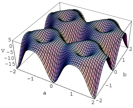
Figure 2: $V_{\rm eff}(a,b)/C$ in (5.21) for $N_{h}=1$ and $N_{f}^{5}=N_{f}^{10}=0$. The global minimum and local minimum are located at $(0,0)$ and $(1,1)$, respectively. The global maxima are located at $(0.4481,0.8096)$, $(0.8096,0.4481)$, $(1.5519,1.1904)$, and $(1.1904,1.5519)$.

As another example, consider a case $N_{h}=1$ and $N_{f}^{5}=N_{f}^{10}=3$. Then $N_{A}=-8$ and $N_{B}=-3$ so that the minimum is found at $(a,b)=(1,1)$. The potential is plotted in fig. 3. The presence of bulk fermions drastically changes the symmetry of the theory.

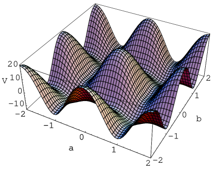
Figure 3: $V_{\rm eff}(a,b)/C$ in (5.21) for $N_{h}=1$ and $N_{f}^{5}=N_{f}^{10}=3$. The global minimum is located at $(1,1)$ whereas $(0,1)$ or $(1,0)$ corresponds to a local minimum. $(0,0)$ is the global maximum.

6.  Phases in the $SU(5)$ theory

The symmetry of the true vacuum for $(N_{h},N_{f}^{5},N_{f}^{10})=(1,0,0)$ or $(1,3,3)$ in the model in the previous section can be found easily. First consider the case $(1,0,0)$. The effective potential has the global minimum at $(a,b)=(0,0)$. The physical symmetry of the theory is the same as the symmetry of the boundary conditions since $(P_{0}^{\rm sym},P_{1}^{\rm sym})=(P_{0},P_{1})$. It is $G_{\rm SM}=SU(3)\times SU(2)\times U(1)$. The extra-dimensional components of the gauge fields $A_{y}^{a}$ ($a=13,\cdots,24$) acquire the common mass $M_{A}$. Recalling $A_{y}^{13}\leftrightarrow a/(gR)$ in (5.5), we find

$$\hskip-28.45274ptM_{A}^{2}=(gR)^{2}~{}{\partial^{2}V_{\rm eff}(a,b)\over\partial a^{2}}\bigg{|}_{a=b=0}={3g^{2}\over 4\pi^{5}R^{3}}~{}\zeta_{R}(3)$$ (6.1)

$$\hskip-5.69046pt={3g_{4}^{2}\over 4\pi^{4}R^{2}}~{}\zeta_{R}(3)~{}~{},$$ (6.2)

where the four-dimensional coupling constant $g_{4}^{2}=g^{2}/(\pi R)$ has been used. A large mass of $O(g_{4}/R)$ has been generated by radiative corrections. As $\raise 0.68889pt\hbox{$\langle$}\lower 0.68889pt\hbox{}A_{y}\,\raise 0.68889pt\hbox{$\rangle$}\lower 0.68889pt\hbox{}=0$, the Higgs field and bulk fermions do not aquire masses by the Hosotani mechanism. Their masses are subject to radiative corrections by other interactions, however.

In the case $(N_{h},N_{f}^{5},N_{f}^{10})=(1,3,3)$ the global minimum of $V_{\rm eff}$ is located at $(1,1)$. The Wilson line phases develop nonvanishing expectation values. As described in Section 2.5, the physical symmetry of the theory is given by (2.47). $(a,b)=(1,1)$ corresponds to

$$\hskip-28.45274pt\hat{w}=2\pi gR\raise 0.68889pt\hbox{$\langle$}\lower 0.68889pt\hbox{}A_{y}\,\raise 0.68889pt\hbox{$\rangle$}\lower 0.68889pt\hbox{}=\pi\pmatrix{0&0&0&1&0\cr 0&0&0&0&1\cr 0&0&0&0&0\cr 1&0&0&0&0\cr 0&1&0&0&0\cr}~{}~{},$$ (6.3)

$$\hskip-28.45274ptW=e^{i\hat{w}}={\rm diag~{}}(-1,-1,1,-1,-1)~{}~{}.$$ (6.4)

Under a gauge transformation $\Omega(y)=\exp\{i(y/2\pi R)\hat{w}\}$, $\raise 0.68889pt\hbox{$\langle$}\lower 0.68889pt\hbox{}A_{y}^{\prime}\,\raise 0.68889pt\hbox{$\rangle$}\lower 0.68889pt\hbox{}=0$ and

$$\hskip-28.45274ptP_{0}^{\rm sym}=P_{0}={\rm diag~{}}(-1,-1,-1,1,1)$$ (6.5)

$$\hskip-28.45274ptP_{1}^{\rm sym}=WP_{1}={\rm diag~{}}(1,1,-1,-1,-1)~{}~{}.$$ (6.6)

The physical symmetry is given by $[SU(2)]^{2}\times[U(1)]^{2}$. The color $SU(3)$ is broken down to $SU(2)\times U(1)$.

At this stage it is appropriate to examine the equivalence classes of boundary conditions in the $SU(5)$ model. The notion of the equivalence class was introduced in Section 2.4, and was claimed in Section 2.5 that theories belonging to the same equivalence class have the same physics as a result of the Hosotani mechanism. We can confirm it in the model under discussions.

Let us consider several boundary conditions belonging to the same equivalence class. Examples are generated by the equivalence relation (2.37) in an $SU(2)$ subspace. The transformation encountered in (6.4) and (6.6) also belong to this category. The examples we consider are

$$({\rm BC}1): P_{0}={\rm diag~{}}(-1,-1,-1,1,1)~{}~{},~{}~{}U={\rm diag~{}}(1,1,1,1,1)~{}~{},$$ (6.9)

$$P_{1}={\rm diag~{}}(-1,-1,-1,1,1)~{}~{},$$

$$\hskip 56.9055ptG_{\rm BC}^{(1)}=SU(3)\times SU(2)\times U(1)$$

$$({\rm BC}2): P_{0}={\rm diag~{}}(-1,-1,-1,1,1)~{}~{},~{}~{}U={\rm diag~{}}(1,-1,1,1,-1)~{}~{},$$ (6.12)

$$P_{1}={\rm diag~{}}(-1,1,-1,1,-1)~{}~{},$$

$$\hskip 56.9055ptG_{\rm BC}^{(2)}=SU(2)\times U(1)\times U(1)\times U(1)$$

$$({\rm BC}3): P_{0}={\rm diag~{}}(-1,-1,-1,1,1)~{}~{},~{}~{}U={\rm diag~{}}(-1,-1,1,-1,-1)~{}~{},$$ (6.15)

$$P_{1}={\rm diag~{}}(1,1,-1,-1,-1)~{}~{},$$

$$\hskip 56.9055ptG_{\rm BC}^{(3)}=SU(2)\times SU(2)\times U(1)\times U(1)$$

$$({\rm BC}4): P_{0}={\rm diag~{}}(-1,-1,-1,1,1)~{}~{},~{}~{}U=P_{1}P_{0}~{}~{},$$ (6.18)

$$P_{1}=\pmatrix{-\cos\pi p&0&0&-i\sin\pi p&0\cr 0&-\cos\pi q&0&0&-i\sin\pi q\cr 0&0&-1&0&0\cr i\sin\pi p&0&0&\cos\pi p&0\cr 0&i\sin\pi q&0&0&\cos\pi q\cr}~{}~{},$$

$$\hskip 56.9055ptG_{\rm BC}^{(4)}=U(1)\times U(1)\times U(1)$$

$G_{\rm BC}$ denotes the symmetry of the boundary conditions at low energies specified by (2.31). (BC1) is Case 2, (5.2). (BC2) and (BC3) are special cases of (BC4) with $(p,q)=(0,1)$ and $(1,1)$, respectively. (BC3) has been encountered in (6.6).

All of the boundary conditions listed in (6.18) belong to the same equivalence class so that the corresponding theories have the same physics. The physical symmetry, $H^{\rm sym}$ defined in (2.47), is determined by the matter content. $H^{\rm sym}=G_{\rm BC}^{(1)}=G_{\rm SM}$ for $(N_{h},N_{f}^{5},N_{f}^{10})=(1,0,0)$, whereas $H^{\rm sym}=G_{\rm BC}^{(3)}$ for $(N_{h},N_{f}^{5},N_{f}^{10})=(1,3,3)$. Although $G_{\rm BC}$’s are different, the theories yield the same physical symmetry by the Hosotani mechanism.

In the rest of this section we shall give detailed accounts of how the cases (BC2), (BC3), and (BC4) lead to the same physics by the dynamics of the Wilson line phases. First we recall that for the boundary conditions (BC1) the effective potential is given by (5.23);

$$\hskip-28.45274ptV_{\rm eff}^{\rm BC1}(a,b)=-C~{}\Bigg{\{}N_{A}\Big{[}f_{5}(a)+f_{5}(b)\Big{]}$$ (6.19)

$$\hskip 28.45274pt+N_{B}~{}\Big{[}f_{5}(a+b)+f_{5}(a-b)\Big{]}+{3\over 2}\Big{[}f_{5}(2a)+f_{5}(2b)\Big{]}~{}\Bigg{\}}~{}~{}.$$ (6.20)

In the case (BC2) there are six degrees of freedom for the Wilson line phases. They are given by

$$A^{0}_{y}={1\over 2gR}\pmatrix{0&\Theta\cr\Theta^{\dagger}&0\cr}~{}~{},~{}~{}\Theta=\pmatrix{\alpha&0\cr 0&\beta\cr\gamma&0\cr}$$ (6.21)

where $\alpha,\beta,\gamma$ are complex. With the aid of the residual symmetry $G_{BC}^{(2)}$ one can take, without loss of generality, $\alpha=a$, $\beta=b$, and $\gamma=0$ ($a,b$: real) for the evaluation of $V_{\rm eff}$. The resultant $A_{y}^{0}$ is the same as (5.5). As described in Appendices C and D, the change in the boundary conditions amounts to the shift $b\rightarrow b-1$ in the spectrum. Hence

$$V_{\rm eff}^{\rm BC2}(a,b)=V_{\rm eff}^{\rm BC1}(a,b-1)~{}~{}.$$ (6.22)

Similarly, in the case (BC3) there remain eight degrees of freedom for the Wilson line phases. They are given by

$$A^{0}_{y}={1\over 2gR}\pmatrix{0&&\Theta\cr&0\cr\Theta^{\dagger}&&0\cr}~{}~{},~{}~{}\Theta=\pmatrix{\alpha&\delta\cr\gamma&\beta\cr}$$ (6.23)

where $\alpha\sim\delta$ are complex. Again with the aid of $G_{BC}^{(3)}$ one can take $\alpha=a$, $\beta=b$, $\gamma=\delta=0$ ($a,b$: real). The resultant $A_{y}^{0}$ is the same as before. In this case the spectrum shifts, from the (BC1) case, as $a\rightarrow a-1$ and $b\rightarrow b-1$ so that

$$V_{\rm eff}^{\rm BC3}(a,b)=V_{\rm eff}^{\rm BC1}(a-1,b-1)~{}~{}.$$ (6.24)

It is easy to generalize the argument. With the boundary condition (BC4) with generic $(p,q)$, there remain only two degrees of freedom for Wilson line phases;

$$A^{0}_{y}={1\over 2gR}\pmatrix{0&&&a\cr&0&&&b\cr&&0\cr a&&&0\cr&b&&&0\cr}$$ (6.25)

where $a,b$ are real. The computation of the effective potential is involved. The detailed accounts are given in appendices A, C and D. It turns out that the shift in the spectrum is summarized by the replacement $a\rightarrow a-p$ and $b\rightarrow b-q$. Consequently

$$V_{\rm eff}^{\rm BC4}(a,b)\equiv V_{\rm eff}^{(p,q)}(a,b)=V_{\rm eff}^{\rm BC1}(a-p,b-q)~{}~{}.$$ (6.26)

This establishes the relation (4.22) in the model under consideration.

Now one can find the physical symmetry. The global minimum of $V_{\rm eff}^{(p,q)}(a,b)$ is located at $(a,b)=(p,q)$ or $(p-1,q-1)$ ($\mbox{mod}~{}1$) for $(N_{h},N_{f}^{5},N_{f}^{10})=(1,0,0)$ or $(1,3,3)$, respectively. In the former case a gauge transformation

$$\Omega(y;p,q)\equiv\exp\bigg{\{}i\,{y\over 2R}\,(p\lambda_{13}+q\lambda_{19})\bigg{\}}$$ (6.27)

brings $\raise 0.68889pt\hbox{$\langle$}\lower 0.68889pt\hbox{}A_{y}\,\raise 0.68889pt\hbox{$\rangle$}\lower 0.68889pt\hbox{}$ to $\raise 0.68889pt\hbox{$\langle$}\lower 0.68889pt\hbox{}A_{y}^{\prime}\,\raise 0.68889pt\hbox{$\rangle$}\lower 0.68889pt\hbox{}=0$. $P_{0}$ remains invariant, whereas $P_{1}$ is transformed back to $P_{1}$ in (BC1). In other words,

$$\hskip-28.45274pt{\rm for~{}}(N_{h},N_{f}^{5},N_{f}^{10})=(1,0,0)$$ (6.28)

$$\hskip-14.22636ptP_{0}^{\rm sym}={\rm diag~{}}(-1,-1,-1,1,1)~{}~{},$$ (6.29)

$$\hskip-14.22636ptP_{1}^{\rm sym}={\rm diag~{}}(-1,-1,-1,1,1)~{}~{},$$ (6.30)

$$\hskip-14.22636ptU^{\rm sym}={\rm diag~{}}(1,1,1,1,1)~{}~{},$$ (6.31)

$$\hskip-14.22636ptH^{\rm sym}=SU(3)\times SU(2)\times U(1)$$ (6.32)

irrespective of the values of $(p,q)$. Similarly, for $(N_{h},N_{f}^{5},N_{f}^{10})=(1,3,3)$ a gauge transformation $\Omega(y;p-1,q-1)$ brings $\raise 0.68889pt\hbox{$\langle$}\lower 0.68889pt\hbox{}A_{y}\,\raise 0.68889pt\hbox{$\rangle$}\lower 0.68889pt\hbox{}$ to $\raise 0.68889pt\hbox{$\langle$}\lower 0.68889pt\hbox{}A_{y}^{\prime}\,\raise 0.68889pt\hbox{$\rangle$}\lower 0.68889pt\hbox{}=0$. The resulting symmetry is

$$\hskip-28.45274pt{\rm for~{}}(N_{h},N_{f}^{5},N_{f}^{10})=(1,3,3)$$ (6.33)

$$\hskip-14.22636ptP_{0}^{\rm sym}={\rm diag~{}}(-1,-1,-1,1,1)~{}~{},$$ (6.34)

$$\hskip-14.22636ptP_{1}^{\rm sym}={\rm diag~{}}(1,1,-1,-1,-1)~{}~{},$$ (6.35)

$$\hskip-14.22636ptU^{\rm sym}={\rm diag~{}}(-1,-1,1,-1,-1)~{}~{},$$ (6.36)

$$\hskip-14.22636ptH^{\rm sym}=SU(2)\times SU(2)\times U(1)\times U(1)$$ (6.37)

independent of $(p,q)$.

As far as two theories belong to the same equivalence class of boundary conditions, the physical symmetry is the same. It is guaranteed by the Hosotani mechanism as stated in Section 2. The symmetry depends on the matter content in the theory. Dynamical rearrangement of gauge symmetry has taken place. We summarize the result in Table I. We remark that the number of Wilson line phases depends on the boundary conditions chosen. This does not mean, however, that the total number of degrees of freedom in the theory varies with the boundary conditions. Wilson line phases are zero modes ($y$-independent modes) in $A_{y}$’s. As explained in Appendix A, some components of $A_{y}$’s have mode expansion in $\big{\{}\cos[(n+p)y/R]\big{\}}$ or $\big{\{}\cos[(n+\hbox{${1\over 2}$}p)y/R]\big{\}}$ when the boundary conditions are given by (BC4) in (6.18). There appear zero modes when $n+p$ or $n+\hbox{${1\over 2}$}p$ can be zero for an integral $n$. The number of degrees of freedom is unchanged as the value of $p$ changes.

matter content	minimum of $V_{\rm eff}$	physical symmetry
$(N_{h},N_{f}^{5},N_{f}^{10})$	$(~{}a~{},~{}b~{})$	$H^{\rm sym}$
$(~{}1~{},~{}0~{},~{}0)$	$(~{}p~{},~{}q~{})$	$SU(3)\times SU(2)\times U(1)$
$(~{}1~{},~{}3~{},~{}3~{})$	$(p-1,q-1)$	$SU(2)\times SU(2)\times U(1)\times U(1)$

Table I: Physical symmetry is summarized in the non-supersymmetric $SU(5)$ theory with the boundary conditions (BC4) in (6.18). The physical symmetry is determined by the matter content, but is independent of the parameters $(p,q)$ in the boundary conditions.

7.  Supersymmetric $SU(5)$ model

In the non-supersymmetric $SU(5)$ gauge theory discussed in the previous sections, the triplet-doublet mass splitting for the Higgs field in the fundamental representation is realized at the tree level by the orbifold boundary condition (5.2). However, we have not taken into account a contribution from the potential $V(\phi,\psi)$ at the tree level. In general, there is a mass term $m_{\phi}^{2}|\phi|^{2}$, which is subject to radiative corrections. It is natural to suppose that the magnitude of $m_{\phi}$ is as big as the unification scale in grand unified theories and can become as large as a cutoff scale by radiative corrections due to inherent quadratic divergences. In these circumstances both triplet and doublet components would acquire large mass corrections, unless fine-tuning of parameters were exercised. One way to preserve the large mass splitting between triplet and doublet Higgs fields at and beyond the tree level is to resort to supersymmetry (SUSY) as Kawamura has proposed in his original $SU(5)$ gauge models on $M^{4}\times(S^{1}/Z_{2})$.[16, 18]. The mass term of Higgs multiplets is forbidden by $U(1)_{R}$ symmetry at the tree level and there is no quadratic divergence to alter the magnitude of scalar masses thanks to SUSY. Bearing these advantages in mind, we shall investigate features of the SUSY $SU(5)$ model with the orbifold boundary condition (5.2).

One general comment is in order. If the boundary conditions (5.2) is adopted, there appear Wilson line degrees of freedom as in the non-supersymmetric theory. There are dynamics of those Wilson line phases. However, if supersymmetry remains exact and unbroken, the effective potential $V_{\rm eff}$ for the Wilson line phases remains flat at the one loop level, i.e. there remain degenerate vacua.

To have nontrivial dynamics supersymmetry must be broken, either spontaneously or by soft breaking terms. On multiply connected manifolds there is a natural way of introducing soft SUSY breaking. Scherk and Schwarz noted that distinct twisting along, say, $S^{1}$, for bosons and fermions can be implemented without spoiling good properties of SUSY theories.[3] This Scherk-Schwarz mechanism can be exploited in theories on $M^{4}\times(S^{1}/Z_{2})$.[30, 20] Takenaga has examined the Hosotani mechanism in supersymmetric gauge theories on $M^{3}\times S^{1}$ with Scherk-Schwarz SUSY breaking.[12] Gersdorff and Quiros have shown that the Scherk-Schwarz SUSY breaking can be realized as the Hosotani mechanism in the gauged supergravity model as well.[31] We shall adopt the Scherk-Schwarz mechanism for the SUSY breaking, which makes the evaluation of the effective potential easy.

We start to specify the content of the SUSY $SU(5)$ model on $M^{4}\times(S^{1}/Z_{2})$. We take, as an example, the model investigated in ref. [20] modified in the orbifold boundary conditions. $N=1$ SUSY in five-dimensional space-time corresponds to $N=2$ SUSY in four-dimensional ones. A five-dimensional gauge multiplet

$${\cal{V}}=(A^{M},\lambda,\lambda^{\prime},\sigma).$$ (7.1)

is decomposed, in four dimensions, to a vector super-field and a chiral super-field

$$V=(A^{\mu},\lambda)~{}~{},~{}~{}\Sigma=(\sigma+iA^{y},\lambda^{\prime})~{}~{}.$$ (7.2)

We introduce hypermultiplets in fundamental representation (5),

$${\cal H}=(h,h^{c}{}^{\dagger},\tilde{h},\tilde{h}^{c}{}^{\dagger})~{}~{},~{}~{}\overline{{\cal H}}=(\overline{h},\overline{h}^{c}{}^{\dagger},\tilde{\overline{h}},\tilde{\overline{h}}^{c}{}^{\dagger})~{}~{},$$ (7.3)

which are decomposed into chiral superfields as

$$\hskip-28.45274ptH=(h,\tilde{h})~{}~{},~{}~{}\overline{H}=(\overline{h},\tilde{\overline{h}})$$ (7.4)

$$\hskip-28.45274ptH^{c}=(h^{c},\tilde{h}^{c})~{}~{},~{}~{}\overline{H^{c}}=(\overline{h}^{c},\tilde{\overline{h}^{c}})$$ (7.5)

where $H$ ($\overline{H}$)and $H^{c}$ ($\overline{H^{c}}$) have conjugated transformation under the gauge group $SU(5)$.

Next we write down boundary conditions for each field based on the boundary conditions (5.2). Under the $Z_{2}$ reflection at $y=0$, each superfield transforms such that

$$\hskip-28.45274pt\pmatrix{V\cr\Sigma\cr}(x,-y)=P_{0}~{}\pmatrix{V\cr-\Sigma\cr}(x,y)~{}P_{0}^{\dagger}$$ (7.6)

$$\hskip-28.45274pt\left(\begin{array}[]{cc}H&\overline{H}\\ H^{c}{}^{\dagger}&\overline{H}^{c}{}^{\dagger}\end{array}\right)(x,-y)=P_{0}\left(\begin{array}[]{cc}H&-\overline{H}\\ -H^{c}{}^{\dagger}&\overline{H}^{c}{}^{\dagger}\end{array}\right)(x,y)~{}~{},$$ (7.11)

where we take the opposite parity between ${\mathcal{H}}$ and $\overline{\mathcal{H}}$. In this case the supersymmetric Higgs mass term called the $\mu$-term can be derived by twisting boundary conditions on $S^{1}$.[20] If the $\mu$ term is induced by another mechanism such as the Giudice-Masiero mechanism,[32] there is no need to assign opposite parity between ${\mathcal{H}}$ and $\overline{\mathcal{H}}$.

For the shift by $2\pi R$ on $S^{1}$, we impose the following boundary condition on each field a la Scherk and Schwarz,[3]

$$\hskip-28.45274ptA^{M}(x^{\mu},y+2\pi R)=U~{}A^{M}(x^{\mu},y)~{}U^{\dagger}~{}~{},$$ (7.12)

$$\hskip-28.45274pt\left(\begin{array}[]{c}\lambda\\ \lambda^{\prime}\end{array}\right)(x,y+2\pi R)=e^{-2\pi i\beta\sigma_{2}}~{}U~{}\left(\begin{array}[]{c}\lambda\\ \lambda^{\prime}\end{array}\right)(x,y)~{}U^{\dagger}~{}~{},$$ (7.17)

$$\hskip-28.45274pt\sigma(x,y+2\pi R)=U~{}\sigma(x,y)~{}U^{\dagger}~{}~{},$$ (7.18)

$$\hskip-28.45274pt\left(\begin{array}[]{cc}h&\overline{h}\\ h^{c}{}^{\dagger}&\overline{h}^{c}{}^{\dagger}\end{array}\right)(x,y+2\pi R)=e^{-2\pi i\beta\sigma_{2}}~{}U~{}\left(\begin{array}[]{cc}h&\overline{h}\\ h^{c}{}^{\dagger}&\overline{h}^{c}{}^{\dagger}\end{array}\right)(x,y)~{}~{},$$ (7.23)

$$\hskip-28.45274pt\left(\begin{array}[]{cc}\tilde{h}&\tilde{\overline{h}}\\ \tilde{h}^{c}{}^{\dagger}&\tilde{\overline{h}^{c}}{}^{\dagger}\end{array}\right)(x,y+2\pi R)=U~{}\left(\begin{array}[]{cc}\tilde{h}&\tilde{\overline{h}}\\ \tilde{h}^{c}{}^{\dagger}&\tilde{\overline{h}^{c}}{}^{\dagger}\end{array}\right)(x,y)~{}~{},$$ (7.28)

where $\sigma_{2}$ is the Pauli matrix in $SU(2)_{R}$. $\beta$ is real. The five-dimensional action possesses $SU(2)_{R}$ symmetry. With a nonvanishing $\beta$, there appear soft SUSY breaking mass terms for gauginos and scalar fields in four-dimensional theory as will be seen below.

Boundary conditions under $Z_{2}$ reflection at $y=\pi R$ follow from (7.11) and (7.28) by use of generic arguments in 2.1.,

$$\hskip-28.45274ptA^{\mu}(x^{\mu},\pi R-y)=P_{1}~{}A^{\mu}(x^{\mu},\pi R+y)~{}P_{1}^{\dagger}~{}~{},$$ (7.29)

$$\hskip-28.45274ptA^{y}(x^{\mu},\pi R-y)=-P_{1}~{}A^{y}(x^{\mu},\pi R+y)~{}P_{1}^{\dagger}~{}~{},$$ (7.30)

$$\hskip-28.45274pt\left(\begin{array}[]{c}\lambda\\ \lambda^{\prime}\end{array}\right)(x,\pi R-y)=e^{-2\pi i\beta\sigma_{2}}~{}P_{1}~{}\left(\begin{array}[]{c}\lambda\\ -\lambda^{\prime}\end{array}\right)(x,\pi R+y)~{}P_{1}^{\dagger}~{}~{},$$ (7.35)

$$\hskip-28.45274pt\sigma(x,\pi R-y)=-P_{1}~{}\sigma(x,\pi R+y)~{}P_{1}^{\dagger}~{}~{},$$ (7.36)

$$\hskip-28.45274pt\left(\begin{array}[]{cc}h&\overline{h}\\ h^{c}{}^{\dagger}&\overline{h}^{c}{}^{\dagger}\end{array}\right)(x,\pi R-y)=e^{-2\pi i\beta\sigma_{2}}~{}P_{1}~{}\left(\begin{array}[]{cc}h&-\overline{h}\\ -h^{c}{}^{\dagger}&\overline{h}^{c}{}^{\dagger}\end{array}\right)(x,\pi R+y)~{}~{},$$ (7.41)

$$\hskip-28.45274pt\left(\begin{array}[]{cc}\tilde{h}&\tilde{\overline{h}}\\ \tilde{h}^{c}{}^{\dagger}&\tilde{\overline{h}^{c}}{}^{\dagger}\end{array}\right)(x,\pi R-y)=P_{1}~{}\left(\begin{array}[]{cc}\tilde{h}&-\tilde{\overline{h}}\\ -\tilde{h}^{c}{}^{\dagger}&\tilde{\overline{h}^{c}}{}^{\dagger}\end{array}\right)(x,\pi R+y)~{}~{},$$ (7.46)

where $P_{1}=P_{1}^{\dagger}=UP_{0}^{\dagger}=UP_{0}$.

From the above boundary conditions (7.11), (7.28) and (7.46), mode expansions of each field are obtained. We adopt the boundary condition (5.2), or (BC1) in (6.18). The components

$$\hskip-28.45274ptA_{\mu}^{a}\quad(a=1\sim 12)~{}~{},~{}~{}A_{y}^{b}~{},~{}\sigma^{b}\quad(b=13\sim 24)~{},$$ (7.47)

$$\hskip-28.45274pt\widetilde{h}_{i}~{},~{}\widetilde{\overline{h}^{c}_{i}}{}^{\dagger}\quad(i=4,5)~{},\quad\widetilde{\overline{h}^{c}_{j}}~{},~{}\widetilde{h}^{c}_{j}{}^{\dagger}\quad(j=1,2,3)$$ (7.48)

have the same expansion as $\Phi^{+}(x,y)$ in (5.4), whereas the components

$$\hskip-28.45274ptA_{\mu}^{b}\quad(b=13\sim 24)~{},\quad A_{y}^{a}~{},\sigma^{a}\quad(a=1\sim 12)$$ (7.49)

$$\hskip-28.45274pt\widetilde{h}_{j}~{},~{}\widetilde{\overline{h}^{c}_{j}}{}^{\dagger}\quad(j=1,2,3)~{},\quad\widetilde{\overline{h}^{c}_{i}}~{},~{}\tilde{h}^{c}_{i}{}^{\dagger}\quad(i=4,5)$$ (7.50)

have the same expansion as $\Phi^{-}(x,y)$ in (5.4). The gaugino and scalar fields have twist in the $SU(2)_{R}$ space. Their mode expansions are of the type discussed in Appendix A. Gauginos are expanded as

$$\hskip-28.45274pt\pmatrix{\lambda^{a}(x,y)\cr{\lambda^{\prime}}^{a}(x,y)\cr}={1\over\sqrt{\pi R}}\sum_{n=-\infty}^{\infty}\lambda^{a}_{n}(x)\pmatrix{\displaystyle\cos{(n+\beta)y\over R}\cr\displaystyle\sin{(n+\beta)y\over R}\cr}~{}~{},$$ (7.51)

$$\hskip-28.45274pt\pmatrix{\lambda^{b}(x,y)\cr{\lambda^{\prime}}^{b}(x,y)\cr}={1\over\sqrt{\pi R}}\sum_{n=-\infty}^{\infty}\lambda^{b}_{n}(x)\pmatrix{\displaystyle\sin{(n-\beta)y\over R}\cr\displaystyle\cos{(n-\beta)y\over R}\cr}~{}~{},$$ (7.52)

for $a=1\sim 12$ and $b=13\sim 24$, whereas Higgs fields are expanded as

$$\hskip-28.45274pt\pmatrix{h_{j}&\overline{h}_{j}\cr h^{c}_{j}{}^{\dagger}&\overline{h}^{c}{}^{\dagger}_{j}\cr}(x,y)={1\over\sqrt{\pi R}}\sum_{n=-\infty}^{\infty}\pmatrix{h_{j,n}(x)\displaystyle\sin{(n-\beta)y\over R}&\overline{h}_{j,n}(x)\displaystyle\cos{(n+\beta)y\over R}\cr h_{j,n}(x)\displaystyle\cos{(n-\beta)y\over R}&\overline{h}_{j,n}(x)\displaystyle\sin{(n+\beta)y\over R}\cr}$$ (7.53)

$$\hskip-28.45274pt\pmatrix{h_{i}&\overline{h}_{i}\cr h^{c}_{i}{}^{\dagger}&\overline{h}^{c}{}^{\dagger}_{i}\cr}(x,y)={1\over\sqrt{\pi R}}\sum_{n=-\infty}^{\infty}\pmatrix{h_{i,n}(x)\displaystyle\cos{(n+\beta)y\over R}&\overline{h}_{i,n}(x)\displaystyle\sin{(n-\beta)y\over R}\cr h_{i,n}(x)\displaystyle\sin{(n+\beta)y\over R}&\overline{h}_{i,n}(x)\displaystyle\cos{(n-\beta)y\over R}\cr}$$ (7.54)

for $j=1,2,3$ and $i=4,5$.

When the above mode expansions are inserted, the following mass terms appear for gauginos and Higgs scalars upon compactification from the kinetic terms of the five-dimensional theory;

$$\hskip-28.45274pt{\cal L}_{\rm soft}={1\over 2}\left(\sum_{a=1}^{12}\sum_{n=-\infty}^{\infty}{n+\beta\over R}(\lambda_{n}^{a})^{2}\right.-\sum_{b=13}^{24}\sum_{n=-\infty}^{\infty}\left.{n-\beta\over R}(\lambda_{n}^{b})^{2}+\mbox{h.c.}\right)$$ (7.55)

$$\hskip 28.45274pt-\sum_{j=1}^{3}\sum_{n=-\infty}^{\infty}\left(\left({n-\beta\over R}\right)^{2}|{h}_{j,n}(x)|^{2}+\right.\left.\left({n+\beta\over R}\right)^{2}|\overline{h}_{j,n}(x)|^{2})\right)$$ (7.56)

$$\hskip 28.45274pt-\sum_{i=4}^{5}\sum_{n=-\infty}^{\infty}\left(\left({n+\beta\over R}\right)^{2}|{h}_{i,n}(x)|^{2}+\right.\left.\left({n-\beta\over R}\right)^{2}|\overline{h}_{i,n}(x)|^{2})\right)~{}~{},$$ (7.57)

where $(\lambda_{n}^{a})^{2}=(\lambda_{n}^{a})_{\alpha}\epsilon^{\alpha\beta}(\lambda_{n}^{a})_{\beta}$. At the same time gauge bosons and Higgsinos acquire masses, $n/R$, upon compactification. Hence the supersymmetry is broken explicitly by the twisted boundary condition in the $SU(2)_{R}$ space on $S^{1}$. The zero modes of gauginos and Higgs scalars, some of which constitute the MSSM, have non-vanishing masses, $\beta/R$. Those masses are interpreted as the soft SUSY breaking masses. If there is an additional $U(1)$ twisting in the flavor $SU(2)$ space of $H_{i}$ and $\overline{H_{i}}$, there appear $\mu$ terms proportional to this $U(1)$ phase.[20] For the sake of simplicity this twisting is suppressed in the present paper.

With all these mode expansions the effective potential at the one loop level is evaluated in a similar manner to that in the nonsupersymmetric model. One finds that

$$\hskip-42.67912ptV_{\rm eff}(a,b)=-2C\Bigg{\{}2(1-N_{h})[f_{5}(a)-{1\over 2}f_{5}(a+2\beta)-{1\over 2}f_{5}(a-2\beta)$$ (7.58)

$$\hskip 42.67912pt+f_{5}(b)-{1\over 2}f_{5}(b+2\beta)-{1\over 2}f_{5}(b-2\beta)]$$ (7.59)

$$\hskip 42.67912pt+2f_{5}(a+b)-f_{5}(a+b+2\beta)-f_{5}(a+b-2\beta)$$ (7.60)

$$\hskip 42.67912pt+2f_{5}(a-b)-f_{5}(a-b+2\beta)-f_{5}(a-b-2\beta)$$ (7.61)

$$\hskip 42.67912pt+f_{5}(2a)-{1\over 2}f_{5}(2(a+\beta))-{1\over 2}f_{5}(2(a-\beta))$$ (7.62)

$$\hskip 42.67912pt+f_{5}(2b)-{1\over 2}f_{5}(2(b+\beta))-{1\over 2}f_{5}(2(b-\beta))\Bigg{\}}$$ (7.63)

$$\hskip-14.22636pt=-2C\sum_{n=1}^{\infty}{1\over n^{5}}(1-\cos 2\pi n\beta)~{}\bigg{\{}2(1-N_{h})(\cos\pi na+\cos\pi nb)$$ (7.64)

$$\hskip 85.35826pt+4\cos\pi na\cos\pi nb+\cos 2\pi na+\cos 2\pi nb\bigg{\}}$$ (7.65)

where $N_{h}$ indicates the number of the set of hyper-multiplets ${\mathcal{H}}+\overline{\mathcal{H}}$. Note that $V_{\rm eff}(a,b)=0$ for $\beta=0$. The global minimum of $V_{\rm eff}$ is located at $(a,b)=(0,0)$ or $(1,1)$ depending on $N_{h}$. The difference in the height of the potential at these two points is

$$\hskip-28.45274ptV_{\rm eff}(0,0)-V_{\rm eff}(1,1)=-16(1-N_{h})C\sum_{n=1}^{\infty}{1\over(2n-1)^{5}}~{}\Big{\{}1-\cos 2\pi(2n-1)\beta\Big{\}}$$ (7.66)

$$\hskip 28.45274pt\sim-32\pi^{2}(1-N_{h})C\beta^{2}\sum_{n=1}^{\infty}{1\over(2n-1)^{3}}\qquad\hbox{for small }\beta~{}.$$ (7.67)

Irrespective of the value of the SUSY breaking parameter $\beta$ the point $(a,b)=(0,0)$ is the global minimum of $V_{\rm eff}(a,b)$ when $N_{h}=0$ and $N_{h}=1$. The numerical study shows that

$$\begin{array}[]{c|c|cc}N_{h}&(a,b)=(0,0)&(a,b)=(1,1)&\\ \cline{1-3}\cr 0&\mbox{global min.}&\mbox{local min.}&\\ 1&\mbox{degenerate global min.}&\mbox{degenerate global min.}&\\ 2\sim 4&\mbox{local min.}&\mbox{global min.}&\\ 5\sim&\mbox{unstable}&\mbox{global min.}&\\ \end{array}$$ (7.73)

for small $|\beta|$. $\beta$ should be of order $10^{-14}$ on the phenomenological ground for the soft SUSY breaking masses to be $O(1)$TeV in Eq.(7.57). In fig. 4 $V_{\rm eff}(a,b)$ for $N_{h}=2$ and $N_{f}^{5}=N_{f}^{10}=0$ is depicted. At the global minimum $(a,b)=(1,1)$ the gauge symmetry is dynamically broken to $SU(2)\times SU(2)\times U(1)\times U(1)$. Color $SU(3)$ is broken, which is unacceptable phenomenologically. In the theory with $N_{h}=1$ and $N_{f}^{5}=N_{f}^{10}=0$, both $(a,b)=(0,0)$ and $(a,b)=(1,1)$ are global minima of the effective potential. At $(a,b)=(0,0)$ the symmetry is $SU(3)\times SU(2)\times U(1)$.

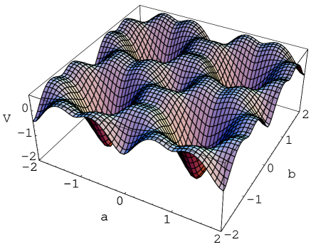
Figure 4: $V_{\rm eff}(a,b)/2C$ in (7.65) for $N_{h}=2$ and $\beta=0.1$ is depicted. The global minimum is located at $(1,1)$ whereas $(0,0)$ corresponds to a local minimum. For $N_{h}=1$ there are degenerate global minima at $(0,0)$ and $(1,1)$.

Physical symmetry is summarized in Table II. No more than one Hyper-multiplet Higgs fields can live in the bulk in the SUSY $SU(5)$ model with the boundary conditions (5.2) to maintain $G_{\rm SM}$ as physical symmetry. To have triplet-doublet splitting, the weak colorless Higgs chiral supermultiplets can be located on the boundary brane not in company with the colored ones, as the gauge symmetry of the four-dimensional boundary brane is not $SU(5)$ but $SU(3)\times SU(2)\times U(1)$. Such an idea for triplet-doublet splitting has been proposed by Hebecker and March-Russell[21] in the scenario that our world is not $SU(5)$-symmetric but $SU(5)$-violating brane in the SUSY SU(5) model equivalent to the one with the boundary conditions (3.2).

Higgs content	minimum of $V_{\rm eff}$	physical symmetry
$N_{h}$	$(a,b)$	$H^{\rm sym}$
$0$	$(~{}0~{},~{}0~{})$	$SU(3)\times SU(2)\times U(1)$
$1$	${\displaystyle(~{}0~{},~{}0~{})\atop\displaystyle(~{}1~{},~{}1~{})}$	${\displaystyle SU(3)\times SU(2)\times U(1)\atop\displaystyle SU(2)\times SU(2)\times U(1)\times U(1)}$
$2$	$(~{}1~{},~{}1~{})$	$SU(2)\times SU(2)\times U(1)\times U(1)$

Table II: Physical symmetry is summarized in the supersymmetric $SU(5)$ theory with the boundary conditions (5.2). The SM gauge symmetry is preserved only when $N_{h}=0$ or $N_{h}=1$.

The mass of $A_{y}^{a}$ $(a=13\sim 24)$ in the $SU(3)\times SU(2)\times U(1)$ vacuum is calculated to be

$$m^{2}=(gR)^{2}{\partial^{2}V_{\rm eff}(a,b)\over\partial a^{2}}\bigg{|}_{a=b=0}\simeq{3g_{4}^{2}\beta^{2}\over 32R^{2}}~{}(5-N_{h})~{}\bigg{(}1-{2\over 3}\log 2\pi\beta\bigg{)}~{}~{},$$ (7.74)

for small $\beta$ where use has been made of

$$\sum_{n=1}^{\infty}{\cos(n\beta)\over n^{3}}\simeq\zeta_{R}(3)+{\beta^{2}\over 2}\log{\beta}-{3\over 4}\beta^{2}~{}.$$ (7.75)

We find that the $A_{y}$ components containing Wilson line degrees of freedom acquire masses by quantum corrections and their magnitude is of order the soft SUSY breaking $\beta/R$. In passing, Eq. (7.74) shows that large $N_{h}\geq 3$ makes the mass square, namely the curvature at origin, be negative, which is consistent with the numerical results in the table in Eq. (7.73).

Before closing this section, we would like to comment on proton stability in this model. We suppose that quarks and leptons are localized on the brane at $y=0$. In the minimal case $N_{h}=0$, there are no dangerous processes inducing proton decay by dimension 5 operators as there lack colored Higgs multiplets. In the case $N_{h}=1$, there may appear colored Higgs multiplets with masses at the TeV scale. Their existence, however, does not threaten the stability of proton thanks to the $U(1)_{R}$ symmetry on the brane. Matter fields have a unit $U(1)_{R}$ charge so that dimension 5 operators such as $[QQQL]_{F}$ and $[\bar{U}\bar{U}\bar{D}\bar{E}]_{F}$ are forbidden. Dimension 4 operators, which trigger rapid proton decay, are also forbidden. The effective dimension 6 operators induced through the exchange of four-dimensional $X$ and $Y$ gauge bosons, $[Q^{\dagger}\bar{U}Q^{\dagger}\bar{E}]_{D}$ and $[Q^{\dagger}\bar{U}L^{\dagger}\bar{D}]_{D}$, are also absent because $X$ and $Y$ gauge bosons do not live in the four-dimensional hypersurface. There are no diagrams involving the exchange of scalar fields $X_{5}^{a}$ and $Y_{5}^{a}$ $(a=13\sim 24)$ unless such light mirror particles as $Q^{c}$ and $L^{c}$ exist on the four-dimensional brane. We conclude that the proton life time is long enough in our model.

We stress that in the SUSY model with $N_{h}=1$, which is most interesting from the phenomenological viewpoint, the color-conserving vacuum is legitimate choice of the nature.

8.  False vacuum decay

In the preceding sections we have found that the effective potential $V_{\rm eff}(a,b)$ is minimized at $(a,b)=(0,0)$ or $(1,1)$, depending on the matter content. The true vacuum corresponds to the global minimum of $V_{\rm eff}(a,b)$. As displayed in figs. 2, 3, and 4 there appears a local minimum of the potential in each case. One may wonder what would happen if the universe were trapped in the local minimum, or in the false vacuum.

The false vacuum would eventually decay to the true vacuum by tunneling. How long does it take before the system decays to settle in the true vacuum? The decay rate is estimated in the semiclassical method.[33] The transition probability per unit volume per unit time is estimated as

$$\frac{\Gamma}{V}\sim Ae^{-S_{E}}$$ (8.1)

where $S_{E}$ is the Euclidean action of the bounce solution. The front coefficient $A$ is $\sim M^{4}$ where $M$ is a typical mass scale of the problem. We shall consider two cases; the nonsupersymmetric and supersymmetric models with $(N_{h},N_{f}^{5},N_{f}^{10})=(1,0,0)$. In the former case $(a,b)=(0,0)$ and $(1,1)$ corresponds to the true and false vacua, respectively. It is the other way around in the latter case.

To find a bounce solution we first note that the size $R$ of the fifth dimension is so small that a bounce solution is expected to be approximately uniform in the fifth dimension. It is four-dimensional. The relevant fields are $A_{y}^{13}$ and $A_{y}^{19}$. As seen from the shape of the potential in fig.  2 or fig. 4, the transition from the false vacuum to the true vacuum takes place mostly along a straight line in the $a$-$b$ space connecting $(0,0)$ and $(1,1)$. Accordingly we restrict ourselves to $A_{y}^{13}=A_{y}^{19}$ and introduce a field $\phi(x)$ by

$$\phi(x)={1\over 2}\,gR\,(A_{y}^{13}+A_{y}^{19})~{}~{}.$$ (8.2)

The bounce solution is a function of $\rho=R^{-1}(x_{1}^{2}+\cdots+x_{4}^{2})^{1/2}$. The relevant part of the effective Euclidean action is

$$\hskip-28.45274ptS_{E}=\int d^{4}x\int_{0}^{\pi R}dy\,\bigg{\{}\frac{1}{2}(\partial_{\mu}A_{y}^{13})^{2}+\frac{1}{2}(\partial_{\mu}A_{y}^{19})^{2}+V_{\rm eff}(A_{y})\bigg{\}}$$ (8.3)

$$\hskip-8.5359pt={4\pi^{2}\over g_{4}^{2}}\int_{0}^{\infty}\rho^{3}d\rho~{}\bigg{\{}{1\over 2}\Big{(}{d\phi\over d\rho}\Big{)}^{2}+U(\phi)\bigg{\}}~{}~{},$$ (8.4)

$$\hskip-28.45274ptU(\phi)={1\over 2}\pi R^{5}g_{4}^{2}~{}V_{\rm eff}(a,b)\Big{|}_{a=b=\phi}~{}~{}.$$ (8.5)

The minima of $U(\phi)$ are located at $\phi=0$ and 1 ($mod$ 2). It is our disposal to normalize $U(\phi)$ such that $U(\phi_{\rm false})=0$.

The Euler-Lagrange equation for $\phi$ is

$$\frac{d^{2}\phi}{d\rho^{2}}+\frac{3}{\rho}\frac{d\phi}{d\rho}=U^{\prime}(\phi)~{}~{},$$ (8.6)

which is equivalent to the equation of motion for a particle in a potential $-U(\phi)$ with friction. The bounce solution needs to satisfy the boundary conditions

$$\hskip-28.45274pt\lim_{\rho\to\infty}\phi(\rho)=\phi_{\rm false}~{}~{},$$ (8.7)

$$\hskip-28.45274pt\frac{d\phi}{d\rho}\,\Bigg{|}_{\rho=0}=0~{}~{}.$$ (8.8)

At $\rho=0$ $\phi$ is at $\phi_{0}$ near $\phi_{\rm true}$. It starts to roll down the hill of the potential $-U(\phi)$, passes the valley, and climbs up the hill to reach $\phi_{\rm false}$ at $\rho=\infty$. The solution can be easily found numerically by the shooting method, which amounts to finding a right value of $\phi_{0}$.

In the non-supersymmetric case $U(\phi)$ is given, from (5.21), by

$$\hskip-28.45274ptU(\phi)={3g_{4}^{2}\over 16\pi^{6}}~{}\widetilde{U}_{1}(\phi)$$ (8.9)

$$\hskip-28.45274pt\widetilde{U}_{1}(\phi)=-[f_{5}(\phi)-f_{5}(1)]-{3\over 4}~{}[f_{5}(2\phi)-f_{5}(0)]~{}~{}.$$ (8.10)

$\widetilde{U}_{1}(\phi)$ has a global minimum at $\phi=0$, a local minimum at $\phi=1$, and a maximum at $\phi=0.6124$. Its values are $\widetilde{U}_{1}(0)=-{31\over 16}\zeta_{R}(5)=-2.00905$, $\widetilde{U}_{1}(1)=0$, and $\widetilde{U}_{1}(0.6124)=0.73749$.

To estimate the tunneling rate we rescale $\rho$ by $z=(3g_{4}^{2}/16\pi^{6})^{1/2}~{}\rho$. Then the equation to be solved becomes

$$\hskip-28.45274pt\frac{d^{2}\phi}{dz^{2}}+\frac{3}{z}\frac{d\phi}{dz}=\widetilde{U}_{1}^{\prime}(\phi)~{}~{},$$ (8.11)

$$\hskip-28.45274pt\phi^{\prime}(0)=0~{}~{},~{}~{}\phi(\infty)=1~{}~{}.$$ (8.12)

The Euclidean action for the bounce is

$$S_{E}={64\pi^{8}\over 3g_{4}^{4}}\int_{0}^{\infty}z^{3}dz~{}\bigg{\{}{1\over 2}\Big{(}{d\phi\over dz}\Big{)}^{2}+\widetilde{U}_{1}(\phi)\bigg{\}}~{}~{}.$$ (8.13)

The equation (8.12) does not contain any parameter. The thin-wall approximation cannot be applied in the problem. As the magnitude of $\widetilde{U}(\phi)$ is $O(1)$, the integral in (8.13) is expected to be $O(1)$. The detailed numerical evaluation shows that the integral is about 1.396. Hence for $g_{4}^{2}/4\pi\sim 1/50$, $S_{E}\sim 4.5\times 10^{7}$. The false vacuum is practically stable. We note that the bounce solution starts at $\phi(0)=3.274\times 10^{-4}$ and make transition in the interval $[1.0,2.5]$ in $z$. The friction term in (8.12) is very effective. The size of the bounce is about $143R$.

In the supersymmetric case $U(\phi)$ is obtained from (7.65). For $N_{h}=2$ and $\beta\ll 1$ it is approximately given by

$$\hskip-28.45274ptU(\phi)\sim{3\beta^{2}g_{4}^{2}\over 8\pi^{4}}~{}\widetilde{U}_{2}(\phi)$$ (8.14)

$$\hskip-28.45274pt\widetilde{U}_{2}(\phi)=f_{3}(\phi)-f_{3}(2\phi)~{}~{}.$$ (8.15)

This time $\widetilde{U}_{2}(\phi)$ has a global minimum at $\phi=1$, a local minimum at $\phi=0$, and a maximum at $\phi=0.3803$. Its values are $\widetilde{U}_{2}(1)=-{7\over 4}\zeta_{R}(3)=-2.1036$, $\widetilde{U}_{2}(0)=0$, and $\widetilde{U}_{2}(0.3803)=0.960244$. After rescaling $z=(3\beta^{2}g_{4}^{2}/8\pi^{4})^{1/2}\rho$, $\phi$ satisfies the same equation as in (8.12) where $\widetilde{U}_{1}$ is replaced by $\widetilde{U}_{2}$. The Euclidean action for the bounce is

$$S_{E}={32\pi^{6}\over 3\beta^{2}g_{4}^{4}}\int_{0}^{\infty}z^{3}dz~{}\bigg{\{}{1\over 2}\Big{(}{d\phi\over dz}\Big{)}^{2}+\widetilde{U}_{2}(\phi)\bigg{\}}~{}~{}.$$ (8.16)

One remark is in order. The potential $\widetilde{U}_{2}(\phi)$ is not regular at $\phi=1$. Its second derivative $\widetilde{U}_{2}^{\prime\prime}(1)$ diverges. The bounce solution starts very close to the true vacuum; $\phi(0)=1-1.0\times 10^{-7}$. It stays near $\phi=1$ for a while, then make a transition to $\phi=0$ in the interval $[1.5,2.3]$ in $z$. Again the friction term in the equation is very effective. The integral in (8.16) is numerically evaluated to be 1.4. $S_{E}$ is large. For $\beta=10^{-2}$ and $g_{4}^{2}/4\pi=1/50$, for instance, $S_{E}\sim 2.3\times 10^{9}$. The size of the bounce is about $(8\pi^{4}/3g_{4}^{2})^{1/2}(R/\beta)$, or $(M_{\rm SUSY})^{-1}$.

The life time of the false vacuum is extremely long. In the SUSY SU(5) model the false vacuum with the $SU(3)\times SU(2)\times U(1)$ symmetry eventually decays into the true vacuum with the $SU(2)\times SU(2)\times U(1)\times U(1)$ symmetry. Its tunneling rate per unit time is $\Gamma\sim 1.04\times 10^{-10^{9}}$ year^-1 for $V=1.7\times 10^{78}$m³, $M=M_{\rm GUT}=10^{16}$GeV, (or $M_{\rm SUSY}=10^{3}$GeV) $\beta=10^{-13}$, and $g_{4}^{2}/4\pi=1/50$. In other words, it is, in practice, stable.

The long life time of the false vacuum originates from the form of the effective potential $V_{\rm eff}$ generated by the dynamics of Wilson line phases, $\theta$’s. The salient feature of $V_{\rm eff}(\theta)$ is that it takes the form $V_{\rm eff}(\theta)=k\,R^{-5}\,\widetilde{U}(\theta)$ where $\widetilde{U}(\theta)$ does not contain any parameters in the theory. The overall coefficient $k$ depends on various parameters in the theory. In four dimensional (low-energy) spacetime small $k$ translates to large $S_{E}$ and longer life time.

9.  Summary and discussions

We have investigated $SU(5)$ gauge theories on $M^{4}\times(S^{1}/Z_{2})$ with particular attention on physics of the orbifold boundary condition and the dynamics of the Wilson lines. First we have given general arguments for classifying the equivalence classes of the boundary conditions, evaluating the effective potential for the left-over Wilson lines, and determining the residual gauge symmetry. These arguments are applicable to theories with arbitrary gauge groups. In particular, the structure of the Hosotani mechanism has been sharpened in (i) $\sim$ (v) of section 2.5. Here we summarize it briefly. ‘Wilson line phases $\theta$’s along non-contractible loops become physical degrees of freedom, whose dynamics selects the physical vacuum configuration minimizing the effective potential $V_{\rm eff}$. If the configuration is nontrivial, the gauge symmetry is either spontaneously broken or enhanced by radiative corrections and gauge fields for broken generators and all extra-dimensional components of gauge fields become massive. Some of matter fields also acquire masses. Rearrangement of gauge symmetry takes place. The physical symmetry of the theory, in general, differs from the symmetry of the boundary conditions. Several sets of boundary conditions having distinct symmetry can be related by boundary-condition-changing gauge transformations, thus belonging to the same equivalence class.’ The Hosotani mechanism guarantees the same physics in each equivalence class. The effective potential $V_{\rm eff}$ , and so do the expectation values of the Wilson line phases. Physical symmetry of the theory is determined by the combination of the boundary conditions and the expectation values of the Wilson line phases. Theories in the same equivalence class of the boundary conditions have the same physical symmetry and physics content.

We have also examined non-SUSY and SUSY $SU(5)$ models on $M^{4}\times(S^{1}/Z_{2})$ to demonstrate rearrangement of gauge symmetry, showing how the symmetry is reduced or enhanced by quantum corrections, depending on the matter content. In the nonsupersymmetric $SU(5)$ model with the boundary conditions (5.2) the minimum of $V_{\rm eff}$ is found at three points, depending on the particle content as shown in (5.32). The physical symmetry is $SU(3)\times SU(2)\times U(1)$ when there are no bulk fermion fields.

The presence of bulk fermions can lead to the spontaneous breaking of color $SU(3)$. Systems with various boundary conditions in (6.18) have been shown to possess the same physics and to be gauge equivalent to each other due to the Hosotani mechanism. We have found that zero modes of the extra-dimensional components, $A_{y}$, of gauge fields acquire masses by radiative corrections. In the supersymmetric model with Scherk-Schwarz SUSY breaking, color $SU(3)$ can be spontaneously broken at the global minimum of $V_{\rm eff}$ if there exist more than one Higgs hypermultiplets ($N_{h}\geq 2$) in the bulk. The zero modes of $A_{y}$’s acquire masses of order of SUSY breaking.

It has been also found that the false vacuum appearing in the model has sufficiently long lifetime, much larger than the age of the universe. It is due to the special form of the effective potential for the dimensionless Wilson line phases.

In this paper we have shown how models with simple boundary conditions have rich structure in the pattern of symmetry breaking/enhancement and mass generation. As an interesting subject, it is yet left over to construct a more realistic grand unified model based on higher-dimensional space-time in which the Hosotani mechanism and the orbifold symmetry breaking conspire to reduce symmetries of the system to those of the standard model. Implementation of the electroweak symmetry breaking is also necessary. Last but not least, our treatment of Higgs fields in the fundamental representation is incomplete in the sense that they have not been unified with gauge fields. With a larger gauge group to start with, all of the Higgs fields in the standard model can be unified in a single gauge field multiplet. We shall come back to these problems in near future.

Acknowledgments

We would like to thank S. Komine, C.S. Lim and K. Oda for many useful discussions. M.H. is grateful to Y. Takubo for his helpful advice in programming. N.H. and Y.H. would like to thank the Summer Institute 2002 held at Fuji-Yoshida for its hospitality where a part of the work was carried out. This work was supported in part by Scientific Grants from the Ministry of Education and Science, Grant No. 13135215, Grant No. 13640284 (M.H. and Y.H.), Grant No. 14039207, Grant No. 14046208,  Grant No. 14740164 (N.H.).

A.  Residual gauge invariance and mode expansion in $SU(2)$ models

It is instructive to classify the residual gauge invariance and mode expansion with orbifold boundary conditions in $SU(2)$ models. The residual gauge invariance is given by (2.28);

$$\hskip-28.45274pt\Omega(x,y+2\pi R)\,U=U\,\Omega(x,y)$$ (A.1)

$$\hskip-28.45274pt\Omega(x,-y)\,P_{0}=P_{0}\,\Omega(x,y)$$ (A.2)

$$\hskip-28.45274pt\Omega(x,\pi R-y)\,P_{1}=P_{1}\Omega(x,\pi R+y)~{}~{}.$$ (A.3)

$P_{0}^{2}=P_{1}^{2}=I$ and $U=P_{1}P_{0}$. One can always diagonalize $P_{0}=P_{0}^{\dagger}$ utilizing global $SU(2)$ invariance.

Case (i)   $P_{0},P_{1}=I$ or $-I$

In this case $U=I$ or $-I$ and the conditions in (A.3) reduce to

$$\Omega(x,y+2\pi R)=\Omega(x,y)~{}~{},~{}~{}\Omega(x,-y)=\Omega(x,y)~{}~{}.$$ (A.4)

There remains the $SU(2)$ gauge invariance.

$$\hskip-28.45274pt\Omega(x,y)=\exp\Big{\{}i\sum_{a=1}^{3}\omega_{a}(x,y)\tau_{a}\Big{\}}$$ (A.5)

$$\hskip-28.45274pt\omega_{a}(x,y)={1\over\sqrt{\pi R}}~{}\omega_{a,0}(x)+\sqrt{{2\over\pi R}}\sum_{n=1}^{\infty}\omega_{a,n}(x)~{}\cos{ny\over R}~{}~{}.$$ (A.6)

$\{\omega_{a,0}(x);a=1,2,3\}$ represents the low energy $SU(2)$ gauge invariance.

Mode expansion in this case is well known. Each component of fields is characterized by the values of $(P_{0},P_{1})$. A field $\phi^{(P_{0},P_{1})}(x,y)$ is expanded as

$$\hskip-28.45274pt\phi^{(++)}(x,y)={1\over\sqrt{\pi R}}~{}\phi_{0}(x)+\sqrt{{2\over\pi R}}\sum_{n=1}^{\infty}\phi_{n}(x)~{}\cos{ny\over R}$$ (A.7)

$$\hskip-28.45274pt\phi^{(--)}(x,y)=\sqrt{{2\over\pi R}}\sum_{n=1}^{\infty}\phi_{n}(x)~{}\sin{ny\over R}$$ (A.8)

$$\hskip-28.45274pt\phi^{(+-)}(x,y)=\sqrt{{2\over\pi R}}\sum_{n=0}^{\infty}\phi_{n}(x)~{}\cos{(n+\hbox{${1\over 2}$})y\over R}$$ (A.9)

$$\hskip-28.45274pt\phi^{(-+)}(x,y)=\sqrt{{2\over\pi R}}\sum_{n=0}^{\infty}\phi_{n}(x)~{}\sin{(n+\hbox{${1\over 2}$})y\over R}~{}~{},$$ (A.10)

where $\pm$ indicates $\pm 1$.

Case (ii)   $P_{0}=I$ or $-I$, and $P_{1}=\tau_{3}$

If $P_{0}\propto I$, $P_{1}$ can be diagonalized by a global $SU(2)$ rotation. One can take without loss of generality $P_{1}=\tau_{3}$ if $P_{1}$ is not proportional to $I$. In this case $U=i\tau_{3}$. The symmetry of the boundary conditions is $U(1)$. The conditions in (A.3) read

$$\Omega(x,y+2\pi R)\tau_{3}=\tau_{3}\Omega(x,y)~{}~{},~{}~{}\Omega(x,-y)=\Omega(x,y)~{}~{}.$$ (A.11)

The residual gauge invariance is given by

$$\hskip-28.45274pt\pmatrix{\omega_{1}(x,y)\cr\omega_{2}(x,y)\cr}=\sqrt{{2\over\pi R}}\sum_{n=0}^{\infty}\pmatrix{\omega_{1,n}(x)\cr\omega_{2,n}(x)\cr}~{}\cos{(n+\hbox{${1\over 2}$})y\over R}$$ (A.12)

$$\hskip-28.45274pt\omega_{3}(x,y)={1\over\sqrt{\pi R}}~{}\omega_{3,0}(x)+\sqrt{{2\over\pi R}}\sum_{n=1}^{\infty}\omega_{3,n}(x)~{}\cos{ny\over R}~{}~{}.$$ (A.13)

where $\omega_{a}$’s are defined in (A.6). $\{\omega_{3,0}(x)\}$ represents the low energy $U(1)$ gauge invariance.

Mode expansion is the same as in Case (i), and is given by (A.10).

Case (iii)   $P_{0}=\tau_{3}$, and $P_{1}=\tau_{3}\,e^{2\pi i(\alpha_{1}\tau_{1}+\alpha_{2}\tau_{2})}$

Without loss of generality we set $\alpha_{1}=0$ and $\alpha_{2}=\alpha$. $U=e^{-2\pi i\alpha\tau_{2}}$. The symmetry of the boundary conditions is minimal; there is none. The conditions in (A.3) are

$$\hskip-28.45274pt\Omega(x,y+2\pi R)=e^{-2\pi i\alpha\tau_{2}}\,\Omega(x,y)\,e^{+2\pi i\alpha\tau_{2}}~{}~{},$$ (A.14)

$$\hskip-28.45274pt\Omega(x,-y)=\tau_{3}\Omega(x,y)\tau_{3}~{}~{},$$ (A.15)

which read

$$\hskip-28.45274pt\omega_{a}(x,-y)=\mp\omega_{a}(x,y)\qquad{\rm for}~{}~{}\cases{a=1,2\cr a=3~{}~{}.\cr}$$ (A.16)

$$\hskip-28.45274pt\omega_{2}(x,y+2\pi R)=\omega_{2}(x,y)$$ (A.17)

$$\hskip-36.98866pt\pmatrix{\omega_{1}(x,y+2\pi R)\cr\omega_{3}(x,y+2\pi R)\cr}=\pmatrix{\cos 4\pi\alpha&\sin 4\pi\alpha\cr-\sin 4\pi\alpha&\cos 4\pi\alpha\cr}\pmatrix{\omega_{1}(x,y)\cr\omega_{3}(x,y)\cr}~{}~{}.$$ (A.18)

The residual gauge symmetry is given by

$$\hskip-28.45274pt\omega_{2}(x,y)=\sqrt{{2\over\pi R}}\sum_{n=1}^{\infty}\omega_{2,n}(x)\sin{ny\over R}$$ (A.19)

$$\hskip-28.45274pt\pmatrix{\omega_{1}(x,y)\cr\omega_{3}(x,y)\cr}={1\over\sqrt{\pi R}}\sum_{n=-\infty}^{\infty}v_{n}(x)\pmatrix{\sin\displaystyle{(n+2\alpha)y\over R}\cr\cos\displaystyle{(n+2\alpha)y\over R}\cr}~{}~{}.$$ (A.20)

The low energy $U(1)$ gauge invariance appears at $\alpha=0,\pm\hbox{${1\over 2}$},\pm 1,\cdots$.

Mode expansion depends on representations in $SU(2)$. For a doublet field $\phi$, or more specifically for

$$\hskip-28.45274pt\phi(x,-y)=\tau_{3}\phi(x,y)~{}~{},$$ (A.21)

$$\hskip-28.45274pt\phi(x,y+2\pi R)=e^{-2\pi i\alpha\tau_{2}}\,\phi(x,y)=\pmatrix{\cos 2\pi\alpha&-\sin 2\pi\alpha\cr\sin 2\pi\alpha&~{}~{}\cos 2\pi\alpha\cr}\,\phi(x,y)$$ (A.22)

the expansion is given by

$$\hskip-28.45274pt\pmatrix{\phi_{1}(x,y)\cr\phi_{2}(x,y)\cr}={1\over\sqrt{\pi R}}\sum_{n=-\infty}^{\infty}\phi_{n}(x)\pmatrix{\cos\displaystyle{(n+\alpha)y\over R}\cr\sin\displaystyle{(n+\alpha)y\over R}\cr}~{}~{}.$$ (A.23)

For a triplet field $\phi_{a}(x,y)$, the expansion is the same as for $\omega_{a}(x,y)$ in (A.20). As the parameter $\alpha$ changes, the mode expansion also changes. When $\alpha$ shifts to $\alpha+1$, $\phi_{n}(x)$ of a doublet field shifts to $\phi_{n-1}(x)$. The resultant spectrum returns to the original one.

The expansion (A.23) with the boundary condition (A.22) constitutes the most typical one. In the computations of the effective potential $V_{\rm eff}(a,b)$ all fields decompose into pairs of the type (A.23).

B.  Generators and structure constants of $SU(5)$

Generators $\Big{\{}~{}\hbox{${1\over 2}$}\lambda_{a}~{};~{}a=1,\cdots,24~{}\Big{\}}$ of $SU(5)$ are given as follows. $\lambda_{3},\lambda_{8},\lambda_{9},\lambda_{12}$ are diagonal matrices given by

$$\hskip-28.45274pt\lambda_{3}={\rm diag~{}}(1,-1,0,0,0)$$ (B.1)

$$\hskip-28.45274pt\lambda_{8}={1\over\sqrt{3}}~{}{\rm diag~{}}(1,1,-2,0,0)$$ (B.2)

$$\hskip-28.45274pt\lambda_{9}={1\over\sqrt{15}}~{}{\rm diag~{}}(2,2,2,-3,-3)$$ (B.3)

$$\hskip-28.45274pt\lambda_{12}={\rm diag~{}}(0,0,0,1,-1)~{}~{}.$$ (B.4)

Other generators are summarized by the following table;

$$\left(\begin{array}[]{ccc|cc}&(1,2)&(4,5)&(13,14)&(15,16)\\ (1,2)&&(6,7)&(17,18)&(19,20)\\ (4,5)&(6,7)&&(21,22)&(23,24)\\ \cline{1-5}\cr(13,14)&(17,18)&(21,22)&&(10,11)\\ (15,16)&(19,20)&(23,24)&(10,11)&\end{array}\right)~{}~{}.$$ (B.10)

Here $(1,2)$, for instance, indicates

$$\lambda_{1}=\left(\begin{array}[]{ccccc}&1&&&\\ 1&&&&\\ &&&&\\ &&&&\\ &&&&\end{array}\right),\;\;\lambda_{2}=\left(\begin{array}[]{ccccc}&-i&&&\\ i&&&&\\ &&&&\\ &&&&\\ &&&&\end{array}\right)~{}~{}.$$ (B.21)

Generators of $G_{\rm SM}=SU(3)\times SU(2)\times U(1)$ are ${\cal G}_{\rm SM}=\Big{\{}~{}\hbox{${1\over 2}$}\lambda_{a}~{};~{}a=1,\cdots,12~{}\Big{\}}$.

In the text and Appendices C and D we need to evaluate eigenvalues of $D^{M}(A^{0})D_{M}(A^{0})$ or $\gamma^{M}D_{M}(A^{0})$ where $A^{0}$ is given by (4.24) and (4.34). As $A^{0}$ is non-vanishing only in the $\lambda_{13}$ and $\lambda_{19}$ components, one needs to know only the structure constants $f_{abc}$’s with $a$ being either 13 or 19. ($f_{abc}$ is normalized such that $[\lambda_{a},\lambda_{b}]=2if_{abc}\lambda_{c}$.) They are given by,

$$\hskip-28.45274ptf_{13,1,18}=f_{13,2,17}=f_{13,3,14}=f_{13,4,22}=f_{13,5,21}$$ (B.22)

$$\hskip 8.5359pt=f_{13,16,10}=f_{13,11,15}=-f_{13,12,14}=-{1\over 2}~{}~{},$$ (B.23)

$$\hskip-28.45274ptf_{19,1,16}=-f_{19,2,15}=-f_{19,3,20}=f_{19,6,24}=f_{19,7,23}$$ (B.24)

$$\hskip 8.5359pt=-f_{19,10,18}=-f_{19,11,17}=-f_{19,20,12}=-{1\over 2}~{}~{},$$ (B.25)

$$\hskip-28.45274ptf_{13,8,14}=f_{19,8,20}=-{1\over 2\sqrt{3}}~{}~{},~{}~{}f_{13,9,14}=f_{19,9,20}=-{\sqrt{5}\over 2\sqrt{3}}~{}~{}.$$ (B.26)

C.  Derivation of $V^{g+gh}_{\rm eff}(a,b)$

In this appendix we derive (5.11) which is the sum of contributions from the gauge fields and the ghost fields in the adjoint representation of $SU(5)$. We present the more general result (6.26) for the boundary condition (BC4) in (6.18). (5.11) corresponds to a special case $p=q=0$ in (BC4).

The evaluation of the effective potential at the one loop level is reduced to finding the excitation spectrum of fields. We start the discussion by examining the spectrum for a pair of fields $\{\phi_{1}(x,y),\phi_{2}(x,y)\}$ subject to the boundary condition (A.22) whose Lagrangian density is given by

$${\cal L}_{\rm pair}={1\over 2}\bigg{(}\partial_{y}\phi_{1}-{\gamma\over R}\phi_{2}\bigg{)}^{2}+{1\over 2}\bigg{(}\partial_{y}\phi_{2}+{\gamma\over R}\phi_{1}\bigg{)}^{2}~{}~{}.$$ (C.1)

Note that ${\cal L}_{\rm pair}(x,-y)={\cal L}_{\rm pair}(x,y)$ and ${\cal L}_{\rm pair}(x,y+2\pi R)={\cal L}_{\rm pair}(x,y)$. Making use of the expansion (A.23), one finds

$$\hskip-28.45274pt\int_{0}^{\pi R}dy\,{\cal L}_{\rm pair}={1\over 4}\int_{-\pi R}^{\pi R}dy\,(\phi_{1},\phi_{2})\pmatrix{-\partial_{y}^{2}+{\displaystyle\gamma^{2}\over\displaystyle R^{2}}&{\displaystyle 2\gamma\over\displaystyle R}\partial_{y}\cr-{\displaystyle 2\gamma\over\displaystyle R}\partial_{y}&-\partial_{y}^{2}+{\displaystyle\gamma^{2}\over\displaystyle R^{2}}\cr}\pmatrix{\phi_{1}\cr\phi_{2}\cr}$$ (C.2)

$$\hskip 0.0pt={1\over 2}\sum_{n=-\infty}^{\infty}{(n+\alpha+\gamma)^{2}\over R^{2}}\,\phi_{n}(x)^{2}~{}~{}.$$ (C.3)

The Kaluza-Klein excitation spectrum in the fifth dimension is $(n+\alpha+\gamma)^{2}/R^{2}$ ($-\infty<n<\infty$), which we symbolically summarize as

$$\big{[}~{}\phi_{1},\phi_{2};\alpha,\gamma~{}\big{]}=\bigg{\{}{(n+\alpha+\gamma)^{2}\over R^{2}}~{};-\infty<n<\infty\bigg{\}}$$ (C.4)

Here $\alpha$ is the boundary condition parameter in (A.22) whereas $\gamma$ represents the amount of mixing caused by nonvanishing Wilson line phases as in (C.1). Note that $[~{}\phi_{1},\phi_{2};\alpha,\gamma~{}]=[~{}\phi_{1},\phi_{2};-\alpha,-\gamma~{}]$.

In (4.14), $V_{\rm eff}[A^{0}]^{g+gh}$ is given by $-(D-2){i\over 2}{\rm Tr\,}\ln D_{L}^{0}D^{0L}$. The trace of operator $D_{L}^{0}D^{0L}$ is evaluated as the sum of its eigenvalues. Hence we must first find the eigenvalues of $D_{L}^{0}D^{0L}=\partial_{\mu}\partial^{\mu}+D_{y}(A_{y}^{0})D_{y}(A_{y}^{0})$ for the adjoint representation. Let us introduce a field $B=\sum_{a}B_{a}{\lambda_{a}\over 2}$ in the adjoint representation. The eigenvalues are found by diagonalizing the bilinear form ${\rm tr}\,(BD_{y}(A^{0})D_{y}(A^{0})B)$ in an appropriate orthogonal basis as given in (A.23). Insertion of $A_{y}^{0}={1\over 2gR}(a\lambda_{13}+b\lambda_{19})$ leads to

$$\hskip-28.45274pt{\cal L}=-{\rm tr\,}(BD_{y}(A^{0})D_{y}(A^{0})B)\sim{\rm tr\,}(\partial_{y}B+ig[A^{0},B])^{2}$$ (C.5)

$$\hskip-14.22636pt={\rm tr\,}\left(\sum_{c}[\partial_{y}B_{c}-{1\over R}\sum_{a,b}f_{abc}\theta_{a}B_{b}]{\lambda_{c}\over 2}\right)^{2}$$ (C.6)

$$\hskip-14.22636pt={1\over 2}\sum_{c=1}^{24}\left(\partial_{y}B_{c}-{a\over R}\sum_{d}f_{13,d,c}B_{d}-{b\over R}\sum_{d}f_{19,d,c}B_{d}\right)^{2}~{}~{}.$$ (C.7)

Making use of (B.26), (C.7) is written as

$$\hskip-28.45274pt{\cal L}={\cal L}_{1}+{\cal L}_{2}+{\cal L}_{4}+{\cal L}_{6}~{}~{},$$ (C.8)

$$\hskip-28.45274pt{\cal L}_{1}={1\over 2}\Big{\{}(\partial_{y}B_{13})^{2}+(\partial_{y}B_{19})^{2}\Big{\}}$$ (C.9)

$$\hskip-28.45274pt{\cal L}_{2}={1\over 2}\bigg{\{}\Big{(}\partial_{y}B_{4}-{a\over 2R}B_{22}\Big{)}^{2}+\Big{(}\partial_{y}B_{22}+{a\over 2R}B_{4}\Big{)}^{2}$$ (C.10)

$$\hskip 14.22636pt+\Big{(}\partial_{y}B_{5}-{a\over 2R}B_{21}\Big{)}^{2}+\Big{(}\partial_{y}B_{21}+{a\over 2R}B_{5}\Big{)}^{2}$$ (C.11)

$$\hskip 14.22636pt+\Big{(}\partial_{y}B_{6}-{b\over 2R}B_{24}\Big{)}^{2}+\Big{(}\partial_{y}B_{24}+{b\over 2R}B_{6}\Big{)}^{2}$$ (C.12)

$$\hskip 14.22636pt+\Big{(}\partial_{y}B_{7}-{b\over 2R}B_{23}\Big{)}^{2}+\Big{(}\partial_{y}B_{23}+{b\over 2R}B_{7}\Big{)}^{2}\bigg{\}}~{}~{},$$ (C.13)

$$\hskip-28.45274pt{\cal L}_{4}={1\over 2}\bigg{\{}\Big{(}\partial_{y}B_{1}-{a\over 2R}B_{18}-{b\over 2R}B_{16}\Big{)}^{2}+\Big{(}\partial_{y}B_{10}+{a\over 2R}B_{16}+{b\over 2R}B_{18}\Big{)}^{2}$$ (C.14)

$$\hskip 14.22636pt+\Big{(}\partial_{y}B_{16}-{a\over 2R}B_{10}+{b\over 2R}B_{1}\Big{)}^{2}+\Big{(}\partial_{y}B_{18}+{a\over 2R}B_{1}-{b\over 2R}B_{10}\Big{)}^{2}$$ (C.15)

$$\hskip 14.22636pt+\Big{(}\partial_{y}B_{2}-{a\over 2R}B_{17}+{b\over 2R}B_{15}\Big{)}^{2}+\Big{(}\partial_{y}B_{11}-{a\over 2R}B_{15}+{b\over 2R}B_{17}\Big{)}^{2}$$ (C.16)

$$\hskip 14.22636pt+\Big{(}\partial_{y}B_{15}+{a\over 2R}B_{11}-{b\over 2R}B_{2}\Big{)}^{2}+\Big{(}\partial_{y}B_{17}+{a\over 2R}B_{2}-{b\over 2R}B_{11}\Big{)}^{2}\bigg{\}}$$ (C.17)

$$\hskip-28.45274pt{\cal L}_{6}={1\over 2}\bigg{\{}\Big{(}\partial_{y}B_{3}-{a\over 2R}B_{14}+{b\over 2R}B_{20}\Big{)}^{2}+\Big{(}\partial_{y}B_{12}+{a\over 2R}B_{14}-{b\over 2R}B_{20}\Big{)}^{2}$$ (C.18)

$$\hskip 14.22636pt+\Big{(}\partial_{y}B_{8}-{a\over 2\sqrt{3}R}B_{14}-{b\over 2\sqrt{3}R}B_{20}\Big{)}^{2}+\Big{(}\partial_{y}B_{9}-{\sqrt{5}\,a\over 2\sqrt{3}R}B_{14}-{\sqrt{5}\,b\over 2\sqrt{3}R}B_{20}\Big{)}^{2}$$ (C.19)

$$\hskip 14.22636pt+\Big{(}\partial_{y}B_{14}+{a\over 2R}B_{3}-{a\over 2R}B_{12}+{a\over 2\sqrt{3}R}B_{8}+{\sqrt{5}\,a\over 2\sqrt{3}R}B_{9}\Big{)}^{2}$$ (C.20)

$$\hskip 14.22636pt+\Big{(}\partial_{y}B_{20}-{b\over 2R}B_{3}+{b\over 2R}B_{12}+{b\over 2\sqrt{3}R}B_{8}+{\sqrt{5}\,b\over 2\sqrt{3}R}B_{9}\Big{)}^{2}~{}\bigg{\}}~{}~{}.$$ (C.21)

We start to evaluate the contributions from ${\cal L}_{2}$. There are four pairs [4-22], [5-21], [6-24], and [7-23]. They are already in the basic form of (A.22) and (C.1). For the [4-22] pair of $A_{\mu}$,

$$\hskip-28.45274pt\pmatrix{B_{4}\cr B_{22}\cr}(x,-y)=\tau_{3}\pmatrix{B_{4}\cr B_{22}\cr}(x,y)$$ (C.22)

$$\hskip-28.45274pt\pmatrix{B_{4}\cr B_{22}\cr}(x,y+2\pi R)=e^{i\pi p\tau_{2}}\pmatrix{B_{4}\cr B_{22}\cr}(x,y)~{}~{}.$$ (C.23)

For the [4-22] pair of $A_{y}$ the $Z_{2}$ parity at $y=0$ is reversed in (C.23), while the $S^{1}$ boundary condition remains the same. The same relations hold for the [5-21] pair. Similar relations hold for the [6-24] pair where $(B_{4},B_{22},p)$ are replaced by $(B_{6},B_{24},q)$ in (C.23). To sum up, we have

$$\hskip-28.45274pt\big{[}~{}B_{4},B_{22};-\hbox{${1\over 2}$}p,\hbox{${1\over 2}$}a~{}\big{]}~{}~{},~{}~{}\big{[}~{}B_{5},B_{21};-\hbox{${1\over 2}$}p,\hbox{${1\over 2}$}a~{}\big{]}$$ (C.24)

$$\hskip-28.45274pt\big{[}~{}B_{6},B_{24};-\hbox{${1\over 2}$}q,\hbox{${1\over 2}$}b~{}\big{]}~{}~{},~{}~{}\big{[}~{}B_{7},B_{23};-\hbox{${1\over 2}$}q,\hbox{${1\over 2}$}b~{}\big{]}~{}~{},$$ (C.25)

for the $A_{\mu}$ and ghost components. For the $A_{y}$ components $[B_{4},B_{22};-\hbox{${1\over 2}$}p,\hbox{${1\over 2}$}a]$, for instance, is replaced by $[B_{22},B_{4};+\hbox{${1\over 2}$}p,-\hbox{${1\over 2}$}a]$. The resulting spectrum is the same as for $A_{\mu}$. Adding the contribution of $\partial_{\mu}\partial^{\mu}$ in the lower four dimensions, one finds that the ${\cal L}_{2}$ part yields

$$2\sum_{n=-\infty}^{\infty}\ln\Bigg{\{}-k^{2}+\left({n-\hbox{${1\over 2}$}p+\hbox{${1\over 2}$}a\over R}\right)^{2}\Bigg{\}}+2\sum_{n=-\infty}^{\infty}\ln\Bigg{\{}-k^{2}+\left({n-\hbox{${1\over 2}$}q+\hbox{${1\over 2}$}b\over R}\right)^{2}\Bigg{\}}~{}.$$ (C.26)

The part ${\cal L}_{4}$ in (C.21) consists of two sets [1-10-16-18] and [2-11-15-17]. Both of them decompose to fundamental pairs. Take the set [1-10-16-18], for example. Introducing

$$C_{\pm}={B_{16}\pm B_{18}\over\sqrt{2}}~{}~{},~{}~{}D_{\pm}={B_{1}\pm B_{10}\over\sqrt{2}}~{}~{},$$ (C.27)

one finds

$$\hskip-42.67912pt{\cal L}_{4}^{\rm[1-10-16-18]}={1\over 2}\bigg{\{}\Big{(}\partial_{y}D_{+}+{a-b\over 2R}C_{-}\Big{)}^{2}+\Big{(}\partial_{y}C_{-}-{a-b\over 2R}D_{+}\Big{)}^{2}$$ (C.28)

$$\hskip 42.67912pt+\Big{(}\partial_{y}D_{-}-{a+b\over 2R}C_{+}\Big{)}^{2}+\Big{(}\partial_{y}C_{+}+{a+b\over 2R}D_{-}\Big{)}^{2}\bigg{\}}~{}~{}.$$ (C.29)

The boundary conditions for the $A_{\mu}$ components are

$$\hskip-28.45274pt\pmatrix{D_{\pm}\cr C_{\mp}\cr}(x,-y)=\tau_{3}\pmatrix{D_{\pm}\cr C_{\mp}\cr}(x,y)$$ (C.30)

$$\hskip-28.45274pt\pmatrix{D_{\pm}\cr C_{\mp}\cr}(x,y+2\pi R)=e^{i\pi(\mp p+q)\tau_{2}}\pmatrix{D_{\pm}\cr C_{\mp}\cr}(x,y)~{}~{}.$$ (C.31)

It follows that

$$\big{[}~{}D_{+},C_{-};\hbox{${1\over 2}$}(p-q),-\hbox{${1\over 2}$}(a-b)~{}\big{]}~{}~{},~{}~{}\big{[}~{}D_{-},C_{+};-\hbox{${1\over 2}$}(p+q),\hbox{${1\over 2}$}(a+b)~{}\big{]}$$ (C.32)

for the $A_{\mu}$ components. The same spectrum holds for the set [2-11-15-17]. The spectrum is unchanged for the $A_{y}$ components as well. The contributions from ${\cal L}_{4}$ are

$$\hskip-28.45274pt2\sum_{n=-\infty}^{\infty}\ln\Bigg{\{}-k^{2}+{1\over R^{2}}\left[~{}n+\hbox{${1\over 2}$}(p+q)-\hbox{${1\over 2}$}(a+b)~{}\right]^{2}\Bigg{\}}$$ (C.33)

$$\hskip 28.45274pt+2\sum_{n=-\infty}^{\infty}\ln\Bigg{\{}-k^{2}+{1\over R^{2}}\left[~{}n+\hbox{${1\over 2}$}(p-q)-\hbox{${1\over 2}$}(a-b)~{}\right]^{2}\Bigg{\}}~{}~{}.$$ (C.34)

${\cal L}_{6}$ in (C.21) simplifies by expressing the diagonal components $B_{3}$, $B_{8}$, $B_{9}$, and $B_{12}$ in an appropriate basis. It is obvious that one should take, instead of (B.4),

$$\hskip-28.45274pt\Lambda_{1}={\rm diag~{}}(1,0,0,-1,0)$$ (C.35)

$$\hskip-28.45274pt\Lambda_{2}={\rm diag~{}}(0,1,0,0,-1)$$ (C.36)

$$\hskip-28.45274pt\Lambda_{3}={1\over\sqrt{2}}~{}{\rm diag~{}}(1,-1,0,1,-1)$$ (C.37)

$$\hskip-28.45274pt\Lambda_{4}={1\over\sqrt{10}}{\rm diag~{}}(1,1,-4,1,1)$$ (C.38)

as a basis for diagonal elements. Accordingly new fields $C_{j}$’s are introduced by

$$C_{1}\Lambda_{1}+C_{2}\Lambda_{2}+C_{3}\Lambda_{3}+C_{4}\Lambda_{4}=B_{3}\lambda_{3}+B_{8}\lambda_{8}+B_{9}\lambda_{9}+B_{12}\lambda_{12}~{}~{},$$ (C.39)

in terms of which ${\cal L}_{6}$ becomes

$$\hskip-42.67912pt{\cal L}_{6}={1\over 2}\bigg{\{}\Big{(}\partial_{y}C_{1}-{a\over R}B_{14}\Big{)}^{2}+\Big{(}\partial_{y}B_{14}+{a\over R}C_{1}\Big{)}^{2}$$ (C.40)

$$\hskip 0.0pt+\Big{(}\partial_{y}C_{2}-{b\over R}B_{20}\Big{)}^{2}+\Big{(}\partial_{y}B_{20}+{b\over R}C_{2}\Big{)}^{2}$$ (C.41)

$$\hskip 0.0pt+(\partial_{y}C_{3})^{2}+(\partial_{y}C_{4})^{2}\bigg{\}}~{}~{}.$$ (C.42)

$(C_{1},B_{14})$ and $(C_{2},B_{20})$ form pairs. Their boundary conditions for $A_{\mu}$’s are

$$\hskip-28.45274pt\pmatrix{C_{1}\cr B_{14}\cr}(x,-y)=\tau_{3}\pmatrix{C_{1}\cr B_{14}\cr}(x,y)~{}~{},$$ (C.43)

$$\hskip-28.45274pt\pmatrix{C_{1}\cr B_{14}\cr}(x,y+2\pi R)=e^{2\pi ip\tau_{2}}\pmatrix{C_{1}\cr B_{14}\cr}(x,y)~{}~{},$$ (C.44)

and

$$\hskip-28.45274pt\pmatrix{C_{2}\cr B_{20}\cr}(x,-y)=\tau_{3}\pmatrix{C_{2}\cr B_{20}\cr}(x,y)~{}~{},$$ (C.45)

$$\hskip-28.45274pt\pmatrix{C_{2}\cr B_{20}\cr}(x,y+2\pi R)=e^{2\pi iq\tau_{2}}\pmatrix{C_{2}\cr B_{20}\cr}(x,y)~{}~{},$$ (C.46)

Contributions from $(C_{1},C_{2},B_{14},B_{20})$ are summarized as

$$\big{[}~{}C_{1},B_{14};-p,a~{}\big{]}~{}~{},~{}~{}\big{[}~{}C_{2},B_{20};-q,b~{}\big{]}$$ (C.47)

so that we have, in the effective potential,

$$\sum_{n=-\infty}^{\infty}\ln\Bigg{\{}-k^{2}+\left({n+p-a\over R}\right)^{2}\Bigg{\}}+\sum_{n=-\infty}^{\infty}\ln\Bigg{\{}-k^{2}+\left({n+q-b\over R}\right)^{2}\Bigg{\}}~{}~{}.$$ (C.48)

Finally contributions from $(B_{13},B_{19})$ in ${\cal L}_{1}$ and $(C_{3},C_{4})$ in ${\cal L}_{6}$ combine to result in a simple form. Their Lagrangian is independent of the Wilson line phases $(a,b)$. All of these fields are periodic on $S^{1}$. For $A_{\mu}$ components, $(B_{13},B_{19})$ has $Z_{2}$ parity $-1$, whereas $(C_{3},C_{4})$ has $+1$. The sign is reversed for $A_{y}$. Hence $(B_{13},B_{19},C_{3},C_{4})$ gives

$$2\sum_{n=-\infty}^{\infty}\ln\Bigg{\{}-k^{2}+{n^{2}\over R^{2}}\Bigg{\}}~{}~{}.$$ (C.49)

Summing (C.26), (C.34), (C.48) and (C.49) and putting $p=q=0$, we have arrived at the expression (5.11). The effective potential for the general boundary condition (BC4) is obtained by replacing $(a,b)$ by $(a-p,b-q)$.

D.  Contributions from fermions in the bulk

Let us consider the case in which there are fermions in the ${\bf 5}$ and ${\bf 10}$ representation of $SU(5)$ propagating in the bulk. They contribute to $V_{\rm eff}$. We shall find that the contribution from the representation ${\bf r}$ is same as that from its conjugate representation $\bar{\bf r}$ as seen from the derivation below.

First we study the contribution from fermions $\psi_{i}(x,y)$, $(i=1,\cdots,5)$ in the ${\bf 5}$ representation. The orbifold boundary conditions are given by

$$\hskip-28.45274pt\psi(x,-y)=\pm P_{0}\gamma^{5}\psi(x,y)$$ (D.1)

$$\hskip-28.45274pt\psi(x,\pi R-y)=\pm e^{i\pi\beta}P_{1}\gamma^{5}\psi(x,\pi R+y)$$ (D.2)

$$\hskip-28.45274pt\psi(x,y+2\pi R)=e^{-i\pi\beta}P_{1}P_{0}\psi(x,y)$$ (D.3)

where $\beta$ is $0$ or $1$. The left and right handed components are defined by $\psi_{L}(x,y)=\hbox{${1\over 2}$}(1-\gamma_{5})\psi(x,y)$ and $\psi_{R}(x,y)=\hbox{${1\over 2}$}(1+\gamma_{5})\psi(x,y)$.

Let us consider the case with the $+$ sign in (D.3). (The formula for the case of the $-$ sign is obtained by interchanging L and R.) For the pair $(\psi_{1},\psi_{4})$ the condition (D.3) reads

$$\hskip-28.45274pt\pmatrix{\psi_{1}\cr i\psi_{4}\cr}(x,-y)=-\tau_{3}\gamma^{5}\pmatrix{\psi_{1}\cr i\psi_{4}\cr}(x,y)$$ (D.4)

$$\hskip-28.45274pt\pmatrix{\psi_{1}\cr i\psi_{4}\cr}(x,y+2\pi R)=e^{-i\pi(p+\beta)\tau_{2}}\pmatrix{\psi_{1}\cr i\psi_{4}\cr}(x,y)~{}~{}.$$ (D.5)

It follows from (A.22) and (A.23) that the fields in the pair are expanded as

$$\hskip-42.67912pt\pmatrix{\psi_{1}(x,y)\cr i\psi_{4}(x,y)\cr}={1\over\sqrt{\pi R}}\sum_{n=-\infty}^{\infty}\Bigg{\{}~{}\psi_{L}^{(n)}(x)\pmatrix{\cos\displaystyle\Big{(}n+\hbox{${1\over 2}$}(p+\beta)\Big{)}{y\over R}\cr\kern 5.0pt\cr\sin\displaystyle\Big{(}n+\hbox{${1\over 2}$}(p+\beta)\Big{)}{y\over R}\cr}$$ (D.6)

$$\hskip 128.0374pt+~{}\psi_{R}^{(n)}(x)\pmatrix{\sin\displaystyle\Big{(}n-\hbox{${1\over 2}$}(p+\beta)\Big{)}{y\over R}\cr\kern 5.0pt\cr\cos\displaystyle\Big{(}n-\hbox{${1\over 2}$}(p+\beta)\Big{)}{y\over R}\cr}~{}\Bigg{\}}~{}~{}.$$ (D.7)

In (4.14), $V_{\rm eff}[A^{0}]^{\rm fermion}$ is given by $-f(D){i\over 2}{\rm Tr\,}\ln D_{L}^{0}D^{0L}$. Eigenvalues of $D_{L}^{0}D^{0L}=\partial_{\mu}\partial^{\mu}-D_{y}^{2}$ in the 1-4 subspace are easily found in the basis of $(\psi_{1},i\psi_{4})$. Notice that

$$\hskip-28.45274pt(\psi\kern-6.49994pt\raise 6.00006pt\hbox{$-$}_{1},\psi\kern-6.49994pt\raise 6.00006pt\hbox{$-$}_{4})(-D_{y}^{2})\pmatrix{\psi_{1}\cr\psi_{4}\cr}$$ (D.8)

$$\hskip-28.45274pt=(\psi\kern-6.49994pt\raise 6.00006pt\hbox{$-$}_{1},-i\psi\kern-6.49994pt\raise 6.00006pt\hbox{$-$}_{4})\pmatrix{-\partial_{y}^{2}+{\displaystyle a^{2}\over\displaystyle 4R^{2}}&-{\displaystyle a\over\displaystyle R}\partial_{y}\cr{\displaystyle a\over\displaystyle R}\partial_{y}&-\partial_{y}^{2}+{\displaystyle a^{2}\over\displaystyle 4R^{2}}\cr}\pmatrix{\psi_{1}\cr i\psi_{4}\cr}$$ (D.9)

which takes the same form as in (C.3). Hence in the notation of (C.4) the spectrum is summarized as

$$\big{[}~{}\psi_{1L},i\psi_{4L};\hbox{${1\over 2}$}(p+\beta),-\hbox{${1\over 2}$}a~{}]~{}~{},~{}~{}\big{[}~{}i\psi_{4R},\psi_{1R};-\hbox{${1\over 2}$}(p+\beta),\hbox{${1\over 2}$}a~{}]~{}.$$ (D.10)

Similarly for the 2-5 components we have

$$\big{[}~{}\psi_{2L},i\psi_{5L};\hbox{${1\over 2}$}(q+\beta),-\hbox{${1\over 2}$}b~{}]~{}~{},~{}~{}\big{[}~{}i\psi_{5R},\psi_{2R};-\hbox{${1\over 2}$}(q+\beta),\hbox{${1\over 2}$}b~{}]~{}.$$ (D.11)

The contribution from $\psi_{3}$ does not contain any dependence on $a$ or $b$. The spectrum is given by $(n+\hbox{${1\over 2}$}\beta)^{2}/R^{2}$ ($n$: integers) after combining contributions from the L and R components. With all these contributions added together each fermion multiplet in 5 yields, for ${\rm Tr\,}\ln D_{M}^{0}D^{0M}$,

$$\hskip-28.45274pt\sum_{n=-\infty}^{\infty}\ln\left\{-k^{2}+\left({n+\hbox{${1\over 2}$}\beta\over R}\right)^{2}\right\}$$ (D.12)

$$\hskip-28.45274pt+2\sum_{n=-\infty}^{\infty}\ln\left\{-k^{2}+\left({n-\hbox{${1\over 2}$}(a-p-\beta)\over R}\right)^{2}\right\}$$ (D.13)

$$\hskip-28.45274pt+2\sum_{n=-\infty}^{\infty}\ln\left\{-k^{2}+\left({n-\hbox{${1\over 2}$}(b-q-\beta)\over R}\right)^{2}\right\}~{}~{}.$$ (D.14)

Next we study the contribution from fermion $\psi_{ij}=-\psi_{ji}$, $(i,j=1,\cdots,5)$ in the ${\bf 10}$ representation. The $Z_{2}$ transformation property is given by

$$\hskip-28.45274pt\psi_{ij}(x,-y)=\pm{(P_{0})_{i}}^{i^{\prime}}{(P_{0})_{j}}^{j^{\prime}}\gamma^{5}\psi_{i^{\prime}j^{\prime}}(x,y)~{}~{},$$ (D.15)

$$\hskip-28.45274pt\psi_{ij}(x,\pi R-y)=\pm e^{i\pi\beta}{(P_{1})_{i}}^{i^{\prime}}{(P_{1})_{j}}^{j^{\prime}}\gamma^{5}\psi_{i^{\prime}j^{\prime}}(x,\pi R+y)~{}~{},$$ (D.16)

$$\hskip-28.45274pt\psi_{ij}(x,y+2\pi R)=e^{-i\pi\beta}{(P_{1}P_{0})_{i}}^{i^{\prime}}{(P_{1}P_{0})_{j}}^{j^{\prime}}\psi_{i^{\prime}j^{\prime}}(x,y)$$ (D.17)

where $\beta$ is either $0$ or $1$. We consider the case with the $+$ sign in (D.8).

The covariant derivative for $\psi_{ij}$ is given by

$$({D_{M}\psi})_{jk}\equiv\partial_{M}\psi_{jk}+ig\Big{\{}{(A_{M})_{j}}^{l}\psi_{lk}+{(A_{M})_{k}}^{l}\psi_{jl}\Big{\}}~{}~{}.$$ (D.18)

The kinetic term is decomposed as

$$\hskip-28.45274pt{1\over 2}\psi\kern-6.49994pt\raise 6.00006pt\hbox{$-$}{}^{ij}i\gamma^{5}(D_{y}\psi)_{ij}={\cal L}_{1}+{\cal L}_{2}+{\cal L}_{4}~{}~{},$$ (D.19)

$$\hskip-28.45274pt{\cal L}_{1}=\psi\kern-6.49994pt\raise 6.00006pt\hbox{$-$}_{14}i\gamma^{5}\partial_{y}\psi_{14}+\psi\kern-6.49994pt\raise 6.00006pt\hbox{$-$}_{25}i\gamma^{5}\partial_{y}\psi_{25}$$ (D.20)

$$\hskip-28.45274pt{\cal L}_{2}=(\psi\kern-6.49994pt\raise 6.00006pt\hbox{$-$}_{34},\psi\kern-6.49994pt\raise 6.00006pt\hbox{$-$}_{13})\,i\gamma^{5}\pmatrix{\partial_{y}&-{\displaystyle ia\over\displaystyle 2R}\cr-{\displaystyle ia\over\displaystyle 2R}&\partial_{y}\cr}\pmatrix{\psi_{34}\cr\psi_{13}\cr}$$ (D.21)

$$\hskip 71.13188pt+(\psi\kern-6.49994pt\raise 6.00006pt\hbox{$-$}_{35},\psi\kern-6.49994pt\raise 6.00006pt\hbox{$-$}_{23})\,i\gamma^{5}\pmatrix{\partial_{y}&-{\displaystyle ib\over\displaystyle 2R}\cr-{\displaystyle ib\over\displaystyle 2R}&\partial_{y}\cr}\pmatrix{\psi_{35}\cr\psi_{23}\cr}~{}~{},$$ (D.22)

$$\hskip-28.45274pt{\cal L}_{4}=(\psi\kern-6.49994pt\raise 6.00006pt\hbox{$-$}_{12},\psi\kern-6.49994pt\raise 6.00006pt\hbox{$-$}_{15},\psi\kern-6.49994pt\raise 6.00006pt\hbox{$-$}_{24},\psi\kern-6.49994pt\raise 6.00006pt\hbox{$-$}_{45})\,i\gamma^{5}\pmatrix{\partial_{y}&{\displaystyle ib\over\displaystyle 2R}&-{\displaystyle ia\over\displaystyle 2R}&0\cr{\displaystyle ib\over\displaystyle 2R}&\partial_{y}&0&{\displaystyle ia\over\displaystyle 2R}\cr-{\displaystyle ia\over\displaystyle 2R}&0&\partial_{y}&-{\displaystyle ib\over\displaystyle 2R}\cr 0&{\displaystyle ia\over\displaystyle 2R}&-{\displaystyle ib\over\displaystyle 2R}&\partial_{y}\cr}\pmatrix{\psi_{12}\cr\psi_{15}\cr\psi_{24}\cr\psi_{45}\cr}~{}~{}.$$ (D.23)

The condition (D.8) for the pair $(\psi_{34},\psi_{13})$ reads

$$\hskip-28.45274pt\pmatrix{\psi_{34}\cr i\psi_{13}\cr}(x,-y)=-\tau_{3}\gamma^{5}\pmatrix{\psi_{34}\cr i\psi_{13}\cr}(x,y)$$ (D.24)

$$\hskip-28.45274pt\pmatrix{\psi_{34}\cr i\psi_{13}\cr}(x,y+2\pi R)=e^{i\pi(p+\beta)\tau_{2}}\pmatrix{\psi_{34}\cr i\psi_{13}\cr}(x,y)~{}~{},$$ (D.25)

which has the same form as (D.5) when $(\psi_{1},\psi_{4},p)$ is replaced by $(\psi_{34},\psi_{13},-p)$. As

$$\hskip-28.45274pt(\psi\kern-6.49994pt\raise 6.00006pt\hbox{$-$}_{34},\psi\kern-6.49994pt\raise 6.00006pt\hbox{$-$}_{13})(-D_{y}^{2})\pmatrix{\psi_{34}\cr\psi_{13}\cr}$$ (D.26)

$$\hskip-28.45274pt=(\psi\kern-6.49994pt\raise 6.00006pt\hbox{$-$}_{34},-i\psi\kern-6.49994pt\raise 6.00006pt\hbox{$-$}_{13})\pmatrix{-\partial_{y}^{2}+{\displaystyle a^{2}\over\displaystyle 4R^{2}}&{\displaystyle a\over\displaystyle R}\partial_{y}\cr-{\displaystyle a\over\displaystyle R}\partial_{y}&-\partial_{y}^{2}+{\displaystyle a^{2}\over\displaystyle 4R^{2}}\cr}\pmatrix{\psi_{34}\cr i\psi_{13}\cr}~{}~{},$$ (D.27)

the spectrum is given by

$$\big{[}~{}\psi_{34L},i\psi_{13L};-\hbox{${1\over 2}$}(p+\beta),\hbox{${1\over 2}$}a~{}]~{}~{},~{}~{}\big{[}~{}i\psi_{13R},\psi_{34R};\hbox{${1\over 2}$}(p+\beta),-\hbox{${1\over 2}$}a~{}]~{}.$$ (D.28)

Similarly we have for the pair $(\psi_{35},\psi_{23})$

$$\big{[}~{}\psi_{35L},i\psi_{23L};-\hbox{${1\over 2}$}(q+\beta),\hbox{${1\over 2}$}b~{}]~{}~{},~{}~{}\big{[}~{}i\psi_{23R},\psi_{35R};\hbox{${1\over 2}$}(q+\beta),-\hbox{${1\over 2}$}b~{}]~{}.$$ (D.29)

${\cal L}_{4}$ in (D.23) is simplified when expressed in terms of

$$E_{\pm}={\psi_{12}\pm\psi_{45}\over\sqrt{2}}~{}~{},~{}~{}F_{\pm}={\psi_{15}\pm\psi_{24}\over\sqrt{2}}~{}~{}.$$ (D.30)

One finds from (D.17) that

$$\hskip-28.45274pt\pmatrix{iF_{-}\cr E_{+}\cr}(x,-y)=-\tau_{3}\gamma^{5}\pmatrix{iF_{-}\cr E_{+}\cr}(x,y)$$ (D.31)

$$\hskip-28.45274pt\pmatrix{iF_{-}\cr E_{+}\cr}(x,y+2\pi R)=e^{i\pi(p+q+\beta)\tau_{2}}\pmatrix{iF_{-}\cr E_{+}\cr}(x,y)~{}~{}.$$ (D.32)

As

$$\hskip-28.45274pt(\overline{F}_{-},\overline{E}_{+})(-D_{y}^{2})\pmatrix{F_{-}\cr E_{+}\cr}$$ (D.33)

$$\hskip-28.45274pt=(-i\overline{F}_{-},\overline{E}_{+})\pmatrix{-\partial_{y}^{2}+\bigg{(}{\displaystyle a+b\over\displaystyle 2R}\bigg{)}^{2}&{\displaystyle a+b\over\displaystyle R}\partial_{y}\cr-{\displaystyle a+b\over\displaystyle R}\partial_{y}&-\partial_{y}^{2}+\bigg{(}{\displaystyle a+b\over\displaystyle 2R}\bigg{)}^{2}\cr}\pmatrix{iF_{-}\cr E_{+}\cr}~{}~{},$$ (D.34)

the spectrum is given by

$$\big{[}~{}iF_{-L},E_{+L};-\hbox{${1\over 2}$}(p+q+\beta),\hbox{${1\over 2}$}(a+b)~{}\big{]}~{}~{},~{}~{}\big{[}~{}E_{+R},iF_{-R};\hbox{${1\over 2}$}(p+q+\beta),-\hbox{${1\over 2}$}(a+b)~{}\big{]}~{}.$$ (D.35)

Relations for the pair $(E_{-},F_{+})$ are obtained by replacing $(E_{+},F_{-};p+q,a+b)$ in (D.32) and (D.34) by $(E_{-},F_{+};-p+q,-a+b)$. The spectrum is given by

$$\big{[}~{}iF_{+L},E_{-L};\hbox{${1\over 2}$}(p-q+\beta),-\hbox{${1\over 2}$}(a-b)~{}\big{]}~{}~{},~{}~{}\big{[}~{}E_{-R},iF_{+R};-\hbox{${1\over 2}$}(p-q+\beta),\hbox{${1\over 2}$}(a-b)~{}\big{]}~{}~{}.$$ (D.36)

The contributions from $(\psi_{14},\psi_{25})$ depend on neither Wilson line phases $a,b$ nor boundary condition parameters $p,q$. Their spectrum is given by $(n+\hbox{${1\over 2}$}\beta)^{2}/R^{2}$ ($n$: integers). With all these contributions added each fermion multiplet in 10 yields, for ${\rm Tr\,}\ln D_{M}^{0}D^{0M}$,

$$\hskip-28.45274pt2\sum_{n=-\infty}^{\infty}\ln\left\{-k^{2}+\left({n+\hbox{${1\over 2}$}\beta\over R}\right)^{2}\right\}$$ (D.37)

$$\hskip-28.45274pt+2\sum_{n=-\infty}^{\infty}\ln\left\{-k^{2}+\left({n-\hbox{${1\over 2}$}(a-p-\beta)}\over R\right)^{2}\right\}$$ (D.38)

$$\hskip-28.45274pt+2\sum_{n=-\infty}^{\infty}\ln\left\{-k^{2}+\left({n-\hbox{${1\over 2}$}(b-q-\beta)}\over R\right)^{2}\right\}$$ (D.39)

$$\hskip-28.45274pt+2\sum_{n=-\infty}^{\infty}\ln\left\{-k^{2}+\left({n-\hbox{${1\over 2}$}(a+b-(p+q)-\beta)}\over R\right)^{2}\right\}$$ (D.40)

$$\hskip-28.45274pt+2\sum_{n=-\infty}^{\infty}\ln\left\{-k^{2}+\left({n-\hbox{${1\over 2}$}(a-b-(p-q)-\beta)}\over R\right)^{2}\right\}~{}~{}.$$ (D.41)

(D.14) and (D.41), after being integrated over $k$, lead to (5.19) for $p=q=0$.

The results in the previous and this appendices show that the effective potential $V_{\rm eff}^{(p,q)}(a,b)$ with the boundary condition (BC4) in (6.18) is a function of $a-p$ and $b-q$, thus establishing (6.26).

References

References

[1]
Th. Kaluza, Sitzungsber, Preuss. Akad. Wiss. Berlin, Phys. Math. Klasse
(1921) 966;
O. Klein, Z. Phys.37 (1926) 895.
[2]
M. B. Green, J. H. Schwarz and E. Witten, Superstring theory I, II,
Cambridge Univ. Press (1987);
J. Polchinski, Superstring theory I, II, Cambridge Univ. Press (1998).
[3]
J. Scherk and J. H. Schwarz,
Phys. Lett. B82 (1979) 60; Nucl. Phys. B153 (1979) 61.
[4]
P. Fayet,
Phys. Lett. B159 (1985) 121; Nucl. Phys. B263 (1986) 649.
[5]
Y. Hosotani, Phys. Lett. B126 (1983) 309.
[6]
Y. Hosotani, Ann. Phys. (N.Y.)190 (1989) 233.
[7]
Y. Hosotani, Phys. Lett. B129 (1984) 193; Phys. Rev. D29 (1984) 731.
[8]
K. Shiraishi, Z. Phys. C35 (1987) 37;
A.T. Davies and A. McLachlan, Phys. Lett. B200 (1988) 305;
Nucl. Phys. B317 (1989) 237;
A. Higuchi and L. Parker, Phys. Rev. D37 (1988) 2853;
J.E. Hetrick and C.L. Ho, Phys. Rev. D40 (1989) 4085;
M. Bergess and D.J. Toms, Phys. Lett. B234 (1990) 97;
A. McLachlan, Nucl. Phys. B338 (1990) 188;
C.L. Ho and Y. Hosotani, Nucl. Phys. B345 (1990) 445.
[9]
K. Ohnishi and M. Sakamoto, Phys. Lett. B486 (2000) 179;
C.C. Lee and C.L. Ho, Phys. Rev. D62 (2000) 085021;
H. Hatanaka, S. Matsumoto, K. Ohnishi, M. Sakamoto,
Phys. Rev. D63 (2001) 105003;
M. Sakamoto and S. Tanimura, Phys. Rev. D65 (2002) 065004;
H. Hatanaka, K. Ohnishi, M. Sakamoto and K. Takenaga,
Prog. Theoret. Phys. 107 (2002) 1191.
[10]
H. Hatanaka, T. Inami and C.S. Lim,
Mod. Phys. Lett. A13 (1998) 2601.
[11]
M. Kubo, C.S. Lim and H. Yamashita,
Mod. Phys. Lett. A17 (2002) 2249.
[12]
K. Takenaga, Phys. Lett. B425 (1998) 114;
Phys. Rev. D58 (1998) 026004;
M. Sakamoto, M. Tachibana and K. Takenaga,
Prog. Theoret. Phys. 104 (2000) 633;
K. Takenaga, Phys. Rev. D64 (2001) 066001; Phys. Rev. D66 (2002) 085009.
[13]
L. J. Dixon, J. A. Harvey, C. Vafa and E. Witten, Nucl. Phys. B261 (1985) 678;
Nucl. Phys. B274 (1986) 285.
[14]
L. Randall and R. Sundrum, Phys. Rev. Lett. 83 (1999) 3370.
[15]
Y. Kawamura, Prog. Theoret. Phys. 103 (2000) 613.
[16]
Y. Kawamura, Prog. Theoret. Phys. 105 (2001) 999.
[17]
Y. Kawamura, Prog. Theoret. Phys. 105 (2001) 691.
[18]
L. Hall and Y. Nomura,
Phys. Rev. D64 (2001) 055003.
[19]
G. Altarelli and F. Feruglio,
Phys. Lett. B511 (2001) 257;
A. B. Kobakhidze,
Phys. Lett. B514 (2001) 131;
Y. Nomura, D. Smith and N. Weiner,
Nucl. Phys. B613 (2001) 147;
A. Hebecker and J. March-Russell,
Nucl. Phys. B625 (2002) 128;
L. J. Hall and Y. Nomura,
Phys. Rev. D65 (2002) 125012;
L. Hall, H. Murayama, and Y. Nomura, Nucl. Phys. B645 (2002) 85;
N. Haba, T. Kondo, Y. Shimizu, T. Suzuki and K. Ukai,
Prog. Theoret. Phys. 106 (2001) 1247;
Y. Nomura,
Phys. Rev. D65 (2002) 085036;
R. Dermisek and A. Mafi,
Phys. Rev. D65 (2002) 055002;
T. Li,
Nucl. Phys.B619 (2001), 75;
Phys. Lett. B520 (2001) 377;
L. J. Hall, Y. Nomura and D. Smith,
Nucl. Phys. B639 (2002) 307;
F. P. Correia, M.. G. Schmidt and Z. Tavartkiladze,
Nucl. Phys. B649 (2003) 39; Phys. Lett. B545 (2002) 153.
[20]
R. Barbieri, L. Hall and Y. Nomura,
Phys. Rev. D66 (2002) 045025; Nucl. Phys. B624 (2002) 63.
[21] A. Hebecker and J. March-Russell,
Nucl. Phys. B613 (2001) 3;
J.A. Bagger and F. Feruglio, Phys. Rev. Lett. 88 (2002) 101601;
C. Biggio and F. Feruglio, Ann. Phys. (N.Y.)301 (2002) 65;
C. Biggio, F. Feruglio, A. Wulzer and F. Zwirner,
JHEP0211 (2002) 13;
T.J. Li, Eur. Phys. J. C24 (2002) 595.
[22]
T. Watari and T. Yanagida, Phys. Lett. B519 (2001) 164;
T. Asaka, W. Buchmüller and L. Covi,
Phys. Lett. B523 (2001) 199;
L. J. Hall, Y. Nomura, T. Okui and D. Smith,
Phys. Rev. D65 (2002) 035008;
L. Hall and Y. Nomura, hep-ph/0205067; hep-ph/0207079;
R. Barbieri, L. Hall, G. Marandella, Y. Nomura, T. Okui, and S. Oliver,
M. Papucci, hep-ph/0208153.
[23]
L. J. Hall, J. March-Russell, T. Okui and D. Smith,
hep-ph/0108161;
N. Haba, Y. Shimizu, T. Suzuki and K. Ukai,
Prog. Theoret. Phys. 107 (2002) 151;
N. Haba, T. Kondo and Y. Shimizu,
Phys. Lett. B531 (2002) 245;
Phys. Lett. B535 (2002) 271;
C. Csaki, C. Grojean, and H. Murayama, hep-ph/0210133.
[24]
G. von Gersdorff, N. Irges and M. Quiros, Nucl. Phys. B635 (2002) 127;
Phys. Lett. B551 (2003) 351;
G. von Gersdorff and M. Quiros, hep-ph/0206029.
[25]
J. E. Hetrick and Y. Hosotani, Phys. Rev. D38 (1988) 2621;
Y. Hosotani and R. Rodriguez, J. Phys. A31 (1998) 9925.
[26]
J. E. Hetrick and Y. Hosotani, Phys. Lett. B230 (1989) 88; J. E. Hetrick, Int. J. Mod. Phys. A9 (1994) 3153.
[27]
Y. Hosotani, Phys. Rev. Lett. 62 (1989) 2785; C.L. Ho and Y. Hosotani, Int. J. Mod. Phys. A7 (1992) 5797.
[28]
N. Arkani-Hamed, A. G. Cohen and H. Georgi, Phys. Lett. B516 (2001) 395;
C. G. Callan and J. A. Harvey, Nucl. Phys. B250 (1985) 427.
[29]
H. D. Kim, J. E. Kim and H. M. Lee, JHEP06 (2002) 48.
[30]
I. Antoniadis,
Phys. Lett. B246 (1990) 377;
I. Antoniadis, C. Munoz, and M. Quiros,
Nucl. Phys. B397 (1993) 515;
A. Pomarol and M. Quiros, Phys. Lett. B438 (1998) 255;
I. Antoniadis, S. Dimopoulos, A. Pomarol and M. Quiros,
Nucl. Phys. B544 (1999) 503;
A. Delgado, A. Pomarol and M. Quiros,
Phys. Rev. D60 (1999) 095008.
[31] G.V. Gersdorff, M. Quiros and A. Riotto, Nucl. Phys. B634 (2002) 90;
G.V. Gersdorff and M. Quiros, Phys. Rev. D65 (2002) 064016.
[32]
G. F. Giudice and A. Masiero,
Phys. Lett. B206 (1988) 480.
[33]
S. Coleman, Phys. Rev. D15 (1977) 2929;
C.G. Callan and S. Coleman, Phys. Rev. D16 (1977) 1762.