Abstract

A non-perturbative approach to Generalized Parton Distributions, and to Deeply Virtual Compton Scattering in particular, based on off mass shell extension of dual amplitudes with Mandelstam analyticity (DAMA) is developed with the spin and helicity structure as well as the threshold behavior accounted for. The model is tested against the data on deep inelastic electron-proton scattering from JLab.

1 Introduction

Parton distributions measure the probability that a quark or gluon carry a fraction $x$ of the hadron momentum. Relevant structure functions (SF) are related by unitarity to the imaginary part of the forward Compton scattering amplitude. Generalized parton distributions (GPD) [1, 2, 3] represent the interference of different wave functions: one, where a parton carries momentum fraction $x+\xi$, and the other one, with momentum fraction $x-\xi$, correspondingly; here $\xi$ is skewedness and can be determined by the external momenta in a deeply virtual Compton scattering (DVCS) experiment. Basically, the DVCS amplitude can be viewed as a binary hadronic scattering amplitude continued off mass shell. DVCS is related to the GPD in the same way as elastic Compton scattering is related to the ordinary SFs.

Apart from the longitudinal momentum fraction of gluons and quarks, GPDs contain also information about their transverse location, given by a Fourier transformation over the $t$-dependent GPD. Real-space images of the target can thus be obtained in a completely new way [4]. Spacial resolution is determined by the virtuality of the incoming photon. Quantum photographs of the nucleons and nuclei with resolutions on the scale of a fraction of femtometer are thus feasible.

One of the first experimental observations of DVCS was based on the recent analysis of the JLab data from the CLAS collaboration. New measurements at higher energies are currently being analyzed, and dedicated experiments are planned [5].

On the theoretical side, much progress has been achieved [1, 2, 3] in treating GPD in the framework of quantum chromodynamics (QCD) and the light-cone technique. On the other hand, non-nonpertubative effects (resonance production, the background, low-$Q^{2}$ effects) dominating the kinematical region of present measurements and the underlying dynamics still leave much ambiguity in the above-mentioned field-theoretical approach. Therefore, as an alternative or complementary approach we have suggested [6, 7, 8] to use dual amplitudes with Mandelstam analyticity (DAMA) as a model for GPD in general and DVCS in particular. We remind that DAMA realizes duality between direct-channel resonances and high-energy Regge behavior (“Veneziano-duality”). By introducing $Q^{2}$-dependence in DAMA, we have extended the model off mass shell and have shown [6, 7] how parton-hadron (or “Bloom-Gilman”) duality is realized in this way. With the above specification, DAMA can serve as and explicit model valid for all values of the Mandelstam variables $s$, $t$ and $u$ as well as any $Q^{2}$, thus realizing the ideas of DVCS and related GPDs. The historical and logical connections between different kinametical regions and relevant models are depicted in Fig. 1.

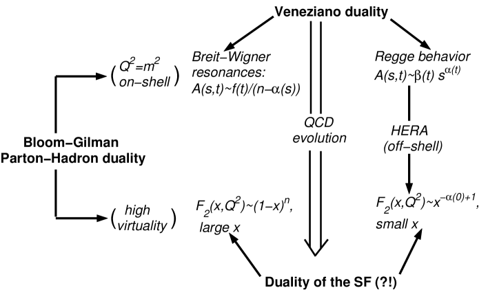
Figure 1.  : Generalized parton distribution amplitudes. A road map.

In this work we concentrate on the very delicate and disputable problem of the off mass shell continuation (introduction of the variable $Q^{2}$) in the dual model, starting with inclusive electron-nucleon scattering both at high energies, typical of HERA, and low energies, with the JLab data in mind (see ref. [8] for more details).

2 Simplified model

The central object of the present study is the nucleon SF, uniquely related to the photoproduction cross section by

$$F_{2}(x,Q^{2})={Q^{2}(1-x)\over{4\pi\alpha(1+{4m^{2}x^{2}\over{Q^{2}}})}}\sigma_{t}^{\gamma^{*}p}(s,Q^{2})\ ,$$ (1)

where the total cross section, $\sigma_{t}^{\gamma^{*}p}$, is the imaginary part of the forward Compton scattering amplitude, $A(s,Q^{2})$, $\sigma_{t}^{\gamma^{*}p}(s)={\cal I}m\ A(s,Q^{2})$; $m$ is the nucleon mass, $\alpha$ is the fine structure constant. The center of mass energy of the $\gamma^{*}p$ system, the negative squared photon virtuality $Q^{2}$ and the Bjorken variable $x$ are related by $s=Q^{2}(1-x)/x+m^{2}$.

We adopt the two-component picture of strong interactions [9], according to which direct-channel resonances are dual to cross-channel Regge exchanges and the smooth background in the $s-$channel is dual to the Pomeron exchange in the $t-$channel. This nice idea, formulated [9] more than three decades ago, was first realized explicitly in the framework of DAMA with nonlinear trajectories (see [11, 6] and earlier references therein).

As explained in Refs. [6] and [11], the background in a dual model corresponds to a pole term with an exotic trajectory that does not produce any resonance.

In the dual-Regge approach [6, 7, 8] Compton scattering can be viewed as an off mass shell continuation of a hadronic reaction, dominated in the resonance region by direct-channel non-strange ($N$ and $\Delta$) baryon trajectories. The scattering amplitude follows from the pole decomposition of a dual amplitude [6]

$$A(s,Q^{2})\Biggl{|}_{t=0}=norm\sum_{i=N_{1}^{*},N_{2}^{*},\Delta,E}A_{i}\sum_{n=n_{i}^{min}}^{n_{i}^{max}}{f_{i}(Q^{2})^{2\left(n-n_{i}^{min}+1\right)}\over{n-\alpha_{i}(s)}}\ ,$$ (2)

where $i$ runs over all the trajectories allowed by quantum number exchange, $norm$ and $A_{i}$’s are constants, $f_{i}(Q^{2})$’s are the form factors. These form factors generalize the concept of inelastic (transition) form factors to the case of continuous spin, represented by the direct-channel trajectories. The $n_{i}^{min}$ refers to the spin of the first resonance on the corresponding trajectory $i$ (it is convenient to shift the trajectories by $1/2$, therefore we use $\alpha_{i}=\alpha^{phys}_{i}-1/2$, which due to the semi-integer values of the baryon spin leaves $n$ in Eq. (2) integer). The sum over $n$ runs with step $2$ (in order to conserve parity).

It follows from Eq. (2) that

$${\cal I}m\ A(s,Q^{2})=norm\sum_{i=N_{1}^{*},N_{2}^{*},\Delta,E}A_{i}\sum_{n=n_{i}^{min}}^{n_{i}^{max}}{[f_{i}(Q^{2})]^{2\left(n-n_{i}^{min}+1\right)}{\cal I}m\ \alpha_{i}(s)\over{(n-{\cal R}e\ \alpha_{i}(s))^{2}+\left({\cal I}m\ \alpha_{i}(s)\right)^{2}}}\ .$$ (3)

TABLE 1.  : Values of the fitted parameters. In the first column we show the result of the fit when the parameters of the baryonic trajectories are fixed. The second column contains the result of the fit when the parameters of the trajectories are varied. ^† denotes the parameters of the physical baryon trajectories from ref. [8]. ^∗ The coefficient $norm$ is chosen in such a way as to keep $A_{N_{1}^{*}}=1$ in order to see the interplay between different resonances.^⋄ Using intercepts and thresholds as a free parameters does not improve the fit, but they may get values far from original.

  $\alpha_{0}$ -0.8377 (fixed)^† -0.8070 -0.8377 (fixed)^⋄ $\alpha_{1}$ 0.95 (fixed)^† 0.9632 0.9842 $N_{1}^{*}$ $\alpha_{2}$ 0.1473 (fixed)^† 0.1387 0.1387 $A_{N_{1}^{*}}$ 1 (fixed)^∗ 1 (fixed)^∗ – $Q^{2}_{N_{1}^{*}}$, GeV² 2.4617 2.6066 –   $\alpha_{0}$ -0.37(fixed)^† -0.3640 -0.37(fixed)^⋄ $\alpha_{1}$ 0.95 (fixed)^† 0.9531 0.9374 $N_{2}^{*}$ $\alpha_{2}$ 0.1471 (fixed)^† 0.1239 0.1811 $A_{N_{2}^{*}}$ 0.5399 0.6086 – $Q^{2}_{N_{2}^{*}}$, GeV² 2.9727 2.6614 –   $\alpha_{0}$ 0.0038 (fixed)^† -0.0065 0.0038 (fixed)^⋄ $\alpha_{1}$ 0.85 (fixed)^† 0.8355 0.8578 $\Delta$ $\alpha_{2}$ 0.1969 (fixed)^† 0.2320 0.2079 $A_{\Delta}$ 4.2225 4.7279 – $Q^{2}_{\Delta}$, GeV² 1.5722 1.4828 –   $s_{0}$, GeV² 1.14 (fixed)^† 1.2871 1.14 (fixed)^⋄       $\alpha_{0}$   0.5645   0.5484   7.576
  $\alpha_{2}$ 0.1126 0.1373 0.0276
${E}$ $s_{E}$, GeV² 1.3086 1.3139 1.311 (fixed)^⋄
$A_{exot}$ 19.2694 14.7267 –
$G_{exot}$ – – 24.16
$Q^{2}_{exot}$, GeV² 4.5259 4.6041 4.910
 DS $Q_{0}^{2}$ – – 2.691
${Q^{\prime}_{0}}^{2}$ – – 0.4114
  $norm$ 0.021 0.0207 0.0659
  $\chi^{2}_{d.o.f.}$ 28.29 11.60 18.1
 

The first three terms in (3) are the non-singlet, or Reggeon contributions with the $N^{*}$ and $\Delta$ trajectories in the $s$-channel, dual to the exchange of an effective bosonic trajectory (essentially, $f$) in the $t$-channel, and the fourth term is the contribution from the smooth background, modeled by a non-resonance pole term with an exotic trajectory $\alpha_{E}(s)$, dual to the Pomeron (see Ref. [6]). As argued in Ref. [6], only a limited number, ${\cal N}$, of resonances appear on the trajectories, for which reason we tentatively set ${\cal N}=3$ - one resonance on each trajectories ($N^{*}_{1},\ N^{*}_{2},\ \Delta$), i.e. $n_{i}^{max}=n_{i}^{min}$. Our analyses [8] shows that ${\cal N}=3$ is a reasonable approximation. The limited (small) number of resonances contributing to the cross section results not only from the termination of resonances on a trajectory but even more due to the strong suppression coming from the numerator (increasing powers of the form factors).

We use Regge trajectories with a threshold singularity and nonvanishing imaginary part in the form:

$$\alpha(s)=\alpha_{0}+\alpha_{1}s+\alpha_{2}(\sqrt{s_{0}}-\sqrt{s_{0}-s}),$$ (4)

where $s_{0}$ is the lightest threshold, $s_{0}=(m_{\pi}+m_{p})^{2}=1.14$ GeV² in our case, and the linear term approximates the contribution from heavy thresholds [6, 7, 8].

For the exotic trajectory we also keep only one term in the sum . $n_{E}^{min}$ is the first integer larger then $Max({\cal R}e\ \alpha_{E})$ – to make sure that there are no resonances on the exotic trajectory. The exotic trajectory is taken in the form

$$\alpha_{E}(s)=\alpha_{E}(0)+\alpha_{1E}(\sqrt{s_{E}}-\sqrt{s_{E}-s})\ ,$$ (5)

where $\alpha_{E}(0)$, $\alpha_{1E}$ and the effective exotic threshold $s_{E}$ are free parameters.

To start with, we use the simplest, dipole model for the form factors, disregarding the spin structure of the amplitude and the difference between electric and magnetic form factors:

$$f_{i}(Q^{2})=\left(1+{Q^{2}/Q^{2}_{0,i}}\right)^{-2}\ ,$$ (6)

where $Q_{0,i}^{2}$ are scaling parameters, determining the relative growth of the resonance peaks and background.

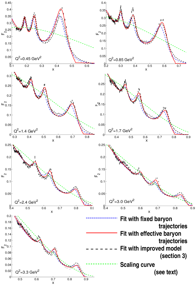
Figure 2.  : $F_{2}$ as a function of $x$ for $Q^{2}=0.45-3.3$ GeV².

We test our model against the experimental data from SLAC [12] and JLab [15]. This set of the experimental data is not homogeneous, i.e. points at low $s$ (high $x$) are given with very small experimental errors, thus “weighting” the fitting procedure not uniformly. Consequently, a preselection of the date involved in the fitting procedure was made, although we present all the experimental points in the Figure. The results of our fits and the values of the fitted parameters are presented in Figs. 2 and Table 1. More details can be found in ref. [8].

For the first fit - first column of Table 1 and dashed-dotted lines in Fig. 2 - we fix the parameters of the $\Delta$ and $N^{*}$ trajectories to the physical ones, reproducing the correct masses and widths of the resonances, leaving the four scaling constants $Q^{2}_{i}$, four factors $A_{i}$ and the parameters of the exotic trajectories to be fitted to the data. Then, to improve the model we effectively account for the large number of overlapping resonances (about 20) present in the energy range under investigation. For this reason we consider the dominant resonances ($N^{*}_{1}$, $N^{*}_{2}$ and $\Delta$) as “effective” contributions to the SF. In other words, we require that they mimic the contribution of the dominant resonances plus the large number of subleading contributions, which, together, fully describe the real physical system. In the light of these considerations, we have refitted the data, allowing the baryon trajectories parameters to vary. The resulting parameters of such a fit are reported in Table 1 (second column). It is worth noting that although the range of variation was not restricted, the new parameters of the trajectories stay close to their physical values, showing stability of the fit and thus reinforcing our previous considerations. From the relevant plots, shown in Fig. 2 with full lines, one can see that the improvement is significant, although agreement is still far from being perfect ($\chi^{2}_{d.o.f.}=11.6$).

The smooth dashed lines in Fig. (2) correspond to a “scaling curves”, i.e. a phenomenological parameterizations of the SF exhibiting Bjorken scaling and fitting the data [10].

3 Spin and helicity; threshold behaviour

In the preceding section the nucleon form factor was treated in a phenomenological way, fitted to the data, neglecting the longitudinal cross section $\sigma_{L}$, and the $Q^{2}\rightarrow 0$ limit of the SFs. On the other hand, it is known [14, 13] that with account for both $\sigma_{L}$ and $\sigma_{T}$ the form factor can be presented as sum o three terms: $G_{+}(Q^{2})$, $G_{0}(Q^{2})$ and $G_{0}(Q^{2}),$ corresponding to $\gamma^{*}N\rightarrow R$ helicity transition amplitudes in the rest frame of the resonance $R$:

$$G_{\lambda_{\gamma}}={1\over m}<R,\lambda_{R}=\lambda_{N}-\lambda_{\gamma}|J(0)|N,\lambda_{N}>;$$ (7)

here $\lambda_{R},\lambda_{N}$ and $\lambda_{\gamma}$ are the resonance, nucleon and photon helicities, $J(0)$ is the current operator; $\lambda_{\gamma}$ assumes the values $-1,0$ and $+1.$ Correspondingly, one replaces the $Q^{2}-$dependent expression in the numerator of (3) by

$$f(Q^{2})^{N}\rightarrow|G_{+}(Q^{2})|^{2}+2|G_{0}(Q^{2})|^{2}+|G_{-}(Q^{2})|^{2}.$$ (8)

The explicit form of these form factors is known only near their thresholds $|\vec{q}|\rightarrow 0$, while their large-$Q^{2}$ behavior may be constrained by the quark counting rules.

According to [16], one has near the threshold

$$G_{\pm}(Q^{2})\sim|\vec{q}|^{J-3/2},\ \ G_{0}(Q^{2})\sim{q_{0}\over{|\vec{q}|}}|\vec{q}|^{J-1/2}$$ (9)

for the so-called normal ($1/2^{+}\rightarrow 3/2^{-},5/2^{+},7/2^{-},...$) transitions and

$$G_{\pm}(Q^{2}\sim|\vec{q}|^{J-1/2},\ \ G_{0}(Q^{2})\sim{q_{0}\over{|\vec{q}|}}|\vec{q}|^{J+1/2}$$ (10)

for the anomalous ($1/2^{+}\rightarrow 1/2^{-},3/2^{+},5/2^{-},...$) transitions, where

$$|\vec{q}|={\sqrt{(M^{2}-m^{2}-Q^{2})^{2}+4M^{2}Q^{2}}\over{2M}},\ \ |\vec{q}|_{Q=0}={M^{2}-m^{2}\over{2M}},$$ (11)

$$q_{0}=\frac{M^{2}-m^{2}-Q^{2}}{2M}\ ,$$ (12)

$M$ is a resonance mass .

Following the quark counting rules, in refs. [13] (for a recent treatment see [14]), the large-$Q^{2}$ behavior of $G$’s was assumed to be

$$G_{+}(Q^{2})\sim Q^{-3},\ \ G_{0}(Q^{2})\sim Q^{-4},\ \ G_{-}(Q^{2})\sim Q^{-5}.$$ (13)

Let us note that while this is reasonable (modulo logarithmic factors) for elastic form factors, it may not be true any more for inelastic (transition) form factors. For example, dual models (see Eq. (1) and ref. [6]) predict powers of the form factors to increase with increasing excitation (resonance spin). This discrepancy can be resolved only experimentally, although a model-independent analysis of the $Q^{2}$-dependence for various nuclear excitations is biased by the (unknown) background.

In ref. [14] the following expressions for the $G$’s, combining the above threshold- (9), (10) with the asymptotic behavior (13), was suggested:

$$|G_{\pm}|^{2}=|G_{\pm}(0)|^{2}\Biggl{(}{|\vec{q}|\over{|\vec{q}|_{Q=0}}}{Q^{\prime 2}_{0}\over{Q^{2}+Q_{0}^{\prime 2}}}\Biggr{)}^{2J-3}\Biggl{(}{Q^{\prime 2}_{0}\over{Q^{2}+Q_{0}^{\prime 2}}}\Biggr{)}^{m_{\pm}}$$ (14)

$$|G_{0}|^{2}=C^{2}\Biggl{(}{Q^{2}_{0}\over{Q^{2}+Q_{0}^{2}}}\Biggr{)}^{2a}{q_{0}^{2}\over{|\vec{q}|^{2}}}\Biggl{(}{|\vec{q}|\over{|\vec{q}|_{Q=0}}}{Q^{\prime 2}_{0}\over{Q^{2}+Q_{0}^{\prime 2}}}\Biggr{)}^{2J-1}\Biggl{(}{Q^{2}_{0}\over{Q^{2}+Q_{0}^{2}}}\Biggr{)}^{m_{0}}$$ (15)

for the normal transitions and

$$|G_{\pm}|^{2}=|G_{\pm}(0)|^{2}\Biggl{(}{|\vec{q}|\over{|\vec{q}|_{Q=0}}}{Q^{\prime 2}_{0}\over{Q^{2}+Q_{0}^{\prime 2}}}\Biggr{)}^{2J-1}\Biggl{(}{Q^{\prime 2}_{0}\over{Q^{2}+Q_{0}^{\prime 2}}}\Biggr{)}^{m_{\pm}}$$ (16)

$$|G_{0}|^{2}=C^{2}\Biggl{(}{Q^{2}_{0}\over{Q^{2}+Q_{0}^{2}}}\Biggr{)}^{2a}\Biggl{(}{q_{0}^{2}\over{|\vec{q}|^{2}}}{Q^{\prime 2}_{0}\over{Q^{2}+Q_{0}^{\prime 2}}}\Biggr{)}^{2J+1}\Biggl{(}{Q^{2}_{0}\over{Q^{2}+Q_{0}^{2}}}\Biggr{)}^{m_{0}}$$ (17)

for the anomalous ones, where $m_{+}=3$, $m_{0}=4$, $m_{-}=5$ count the quarks, $C$ and $a$ are free parameters. The form factors at $Q^{2}=0$ are related to the known (measurable) helicity photoproduction amplitudes $A_{1/2}$ and $A_{3/2}$ by

$$|G_{+,-}(0)|=\frac{1}{\sqrt{4\pi\alpha}}\sqrt{M\over{M-m}}|A_{1/2,3/2}|.$$ (18)

The values of the helicity amplitudes are quoted by experimentalists [17] (those relevant to the present discussion are compiled also in [14]).

We have fitted the above model to the JLab data [15] again by keeping the contribution from three prominent resonances, namely $\Delta(1232)$, $N^{*}(1520)$ and $N^{*}(1680)$. For the sake of simplicity we neglected the cross term containing $G_{0}$ (and the coefficient $C$ and parameter $a$), since it is small relative to the other two terms in Eq. (8) [14].

We use the same background term as in the previous section, but with the normalization coefficient $G_{E}$:

$${background}={{f_{E}}{I_{E}}\over{(n_{E}^{min}-R_{E})^{2}}+I_{E}^{2}}\ ,\ \ {f_{E}}=G_{E}\Biggl{(}{{Q^{2}_{E}}\over{Q^{2}+Q^{2}_{E}}}\Biggr{)}^{4}\ .$$

To be specific, we write explicitly the three resonance terms, to be fitted to the data, (cf. with Eq. (3) of the previous section):

$${\cal I}m\ A(s,Q^{2})=norm\cdot$$

$${f_{\Delta}I_{\Delta}\over{(1-R_{\Delta})^{2}+I_{\Delta}^{2}}}+{f_{N^{-}}I_{N^{-}}\over{(1-R_{N^{-}})^{2}+I_{N^{-}}^{2}}}+{f_{N^{+}}I_{N^{+}}\over{(2-R_{N^{+}})^{2}+I_{N^{+}}^{2}}}+background,$$ (19)

where e.g. $f_{\Delta}$ is calculated according to Eqs. (8,14,16):

$$f_{\Delta}=\Biggl{(}{|\vec{q}|\over{|\vec{q}|_{Q=0}}}{Q^{\prime 2}_{0}\over{Q^{2}+Q_{0}^{\prime 2}}}\Biggr{)}^{2J-1=2}\Biggl{(}|G_{+}(0)|^{2}\Bigl{(}{Q^{2}_{0}\over{Q^{2}+Q_{0}^{2}}}\Bigr{)}^{3}+|G_{-}(0)|^{2}\Biggl{(}{Q^{2}_{0}\over{Q^{2}+Q_{0}^{2}}}\Bigr{)}^{5}\Biggr{)};$$ (20)

here $R$ and $I$ denote the real and the imaginary parts of the relevant trajectory, specified by the subscript. Similar expressions can be easily cast for $f_{N^{+}}$ and for $f_{N^{-}}$ as well.

The form factors at $Q^{2}=0$ can be simply calculated from Eq. (18) by inserting the known [17] (see also Table 1 in [14]) values of the relevant photoproduction amplitudes:

$A_{\Delta(1232)}(1/2,3/2)=(-0.141\ GeV^{-1/2},-0.258\ GeV^{-1/2});$

$A_{N(1520))}(1/2,3/2)=(-0.022\ GeV^{-1/2},0.167\ GeV^{-1/2})$;

$A_{N(1680)}(1/2,3/2)=(-0.017\ GeV^{-1/2},0.127\ GeV^{-1/2}).$

Note that in this way the relative normalization of the resonance terms is fixed (no $A_{i}$’s appearing in previous section), leaving only two adjustable parameters, $Q_{0}^{2}$ and $Q^{\prime 2}_{0}$ (provided $C$ is set zero, then $a$ also disappears), which means that this version of the model (with the cross term, containing $G_{0}$, neglected!) is very restrictive.

The resulting fits to the SLAC and JLab data are presented in Fig. 2 (dashed lines) and Table 1 (third column). The fit is not so good ($\chi^{2}_{d.o.f.}=18.1$), what probably tells us not to neglect the cross term. We hope to account for this and to improve the fit in the forthcoming works.

4 Future Prospects

In this work we have presented new results on the extension of a dual model (Sec. 2) to include the spin and helicity structure of the amplitudes (SFs) as well as its threshold behavior as $Q^{2}\rightarrow 0$. Let us remind that the lowest threshold (in the direct channel) of a hadronic reaction (if Compton scattering is considered in analogy with $\pi N$ scattering) is $s_{0}=(m_{\pi}+m_{N})^{2}$. Hence its imaginary part and the relevant structure function starts at this value and vanishes below $s_{0}$. The “gap” between the lowest electromagnetic $m_{p}^{2}$ and the above-mentioned hadronic thresholds is filled by the arguments and formulas of Sec. 3. The $Q^{2}\rightarrow 0$ is also important as the transition point between elastic and inelastic dynamics.

The important step performed in our work after Ref. [14] is the “Reggization” of the Breit-Wigner pole terms (19), i.e. single resonance terms in Ref. [14] are replaced by those including relevant baryon trajectories. The form of these trajectories, constrained by analyticity, unitarity and by the experimental data is crucial for the dynamic. The use of baryon trajectories instead of individual resonances not only makes the model economic (several resonances are replaced by one trajectory) but also helps in classifying the resonances, by including the “right” ones and eliminating those nonexistent. The construction of feasible models of baryon trajectories, fitting the data on resonances and yet satisfying the theoretical bounds, is in progress.

Note also that the dual model constrains the form factors: as seen from Eq. (3), the powers of the form factors rise with increasing spin of the excited state. This property of the model can and should be tested experimentally.

The $Q^{2}$ dependence, introduced in this model via the form factors can be studied and constrained also by means of the QCD evolution equations.

To summarize, the model presented in this paper, can be used as a laboratory for testing various ideas of the analytical S-matrix and quantum chromodynamics. Its virtue is a simple explicit form, to be elaborated and constrained further both by theory and experimental tests.

Acknowledgment. L.J., A.L. and V.M. acknowledge the support by INTAS, grants 00-00366 and 97-31726.

References

- [1] Müller, D. et al. (1994) Wave Functions, Evolution Equations and Evolution Kernels from Light-Ray Operators of QCD, Fortschr. Phys. 42 pp. 101-142.
- [2] Ji, X. (1997) Gauge invariant decomposition of nucleon spin and its spin-off, Phys. Rev. Lett. 78 pp. 610-613.
- [3] Radyushkin, A.V. (1996) Scaling limit of deeply virtual Compton scattering, Phys. Lett. B380 pp. 417-425; (1997) Nonforward parton distributions, Phys. Rev. D56 pp. 5524-5557.
- [4] Pire, B. (2002) Generalized Parton Distributions and Generalized Distribution Amplitudes : New Tools for Hadronic Physics, hep-ph/0211093.
- [5] Elouadrhirs, L., (2002) Deeply Virtual Compton Scattering at Jefferson Lab, Results and Prospects, hep-ph/0210341.
- [6] Jenkovszky, L.L., Magas, V.K., Predazzi, E. (2001) Resonance-reggeon and parton-hadron duality in strong interactions, Eur. Phys. J., A12, pp. 361-367;
- [7] Jenkovszky, L.L., Magas, V.K., Predazzi, E. Duality in strong interactions, nucl-th/0110085; Jenkovszky, L.L., Magas, V.K., Dual Properties of the Structure Functions, hep-ph/0111398, Proceedings of the 31st International Symposium On Multiparticle Dynamics (ISMD 2001) , September 1-7, 2001, Datong, China, pp. 74-77;
- [8] Fiore, R. et al. (2002) Explicit model realizing parton-hadron duality, hep-ph/0206027, to appear in Eur. Phys. J A.
- [9] Freund, P. (1968) Finite energy sum rules and bootstraps, Phys. Rev. Lett., 20, pp. 235-237; Harari, H. (1968) Pomeranchuk trajectory and its relation to low-energy scattering amplitudes, Phys. Rev. Lett., 20, pp. 1395-1398.
- [10] Csernai, L.P. et al. (2002) From Regge Behavior to DGLAP Evolution Eur. Phys. J. C24 (2002) pp. 205-211.
- [11] Jenkovszky, L.L., Kononenko, S.Yu., Magas, V.K (2002) Diffraction from the direct-channel point of view: the background, hep-ph/0211158.
- [12] Stoler, P. (1991) Form-factors of excited baryons at high Q**2 and the transition to perturbative QCD, Phys. Rev. Lett. 66 pp. 1003-1006; (1991) Form-factors of excited baryons at high Q**2 and the transition to perturbative QCD. 2., Phys. Rev. D44 pp. 73-80.
- [13] Carlson, C.E., Mukhopadhyay, N.C. (1995) Leading log effects in the resonance electroweak form-factors, Phys. Rev. Lett. 74 pp. 1288-1291; (1998) Bloom-Gilman duality in the resonance spin structure functions, Phys. Rev. D58 094029.
- [14] Davidovsky, V.V. and Struminsky, B.V. (2002) The Behavior of Form Factors of Nucleon Resonances and Quark-Hadron Duality, hep-ph/0205130 and in these Proceedings.
- [15] http://www.jlab.org/resdata.
- [16] Bjorken, J.D. and Walecka, J.D., (1966) Electroproduction of nucleon resonances Ann. Physics 38 pp. 35-62.
- [17] Particle Data Group (1998) Eur. Phys. J C3 pp.1-794.