IPPP/02/70

DCPT/02/140

On supersymmetric contributions to the CP asymmetry of the $B\to\phi K_{S}$

 

Abstract

We analyse the CP asymmetry of the $B\to\phi K_{S}$ process in general supersymmetric models. In the framework of the mass insertion approximation, we derive model independent limits for the mixing CP asymmetry. We show that chromomagnetic type of operator may play an important role in accounting for the deviation of the mixing CP asymmetry between $B\to\phi K_{S}$ and $B\to J/\psi K_{S}$ processes observed by Belle and BaBar experiments. A possible correlation between the direct and mixing CP asymmetry is also discussed. Finally, we apply our result in minimal supergravity model and supersymmetric models with non-universal soft terms.

 

1 Introduction

With the advent of experimental data from the $B$ factories, the Standard Model (SM) will be subject to a very stringent test, with the potential for probing virtual effects from new physics. Measurements of the CP asymmetries in various processes are at the center of attentions since in the SM, all of them have to be consistently explained by a single parameter, the phase in the Cabbibo–Kobayashi–Maskawa mixing matrix $\delta_{KM}$  [1].

The BaBar [2] and Belle [3] measurements of time dependent asymmetry in $B\to J/\psi K_{S}$ have provided the first evidence for the CP violation in the $B$ system. The world average of these results, $S_{J/\psi K_{S}}=\sin 2\beta(2\phi_{1})=0.734\pm 0.054$, is in a good agreement with the SM prediction. Therefore, one may have already concluded that the KM mechanism is the dominant source of the CP violation in $B$ system. However, in the $B\to J/\psi K_{S}$ process, new physics (NP) effects enter only at the one loop level while the SM contributions has dominant tree level contributions. Thus, it is natural that NP does not show up clearly in this process. In fact, in order that a significant supersymmetric contribution appear to $S_{J/\psi K_{S}}$, we need a large flavour structure and/or large SUSY CP violating phases, which usually do not exist in most of the supersymmetric models such as SUSY models with minimal flavour violation or SUSY models with non-minimal flavour and hierarchical Yukawa couplings (see Ref. [4] more in detail).

Unlike the $B\to J/\psi K_{S}$ process, $B\to\phi K_{S}$ is induced only at the one loop level both in SM and NP. Thus, it is tempting to expect that the SUSY contributions to this decay are more significant [5, 6, 7, 8]. Based on the KM mechanism of CP violation, both CP asymmetries of $B\to\phi K_{S}$ and $B\to J/\psi K_{S}$ processes should measure $\sin 2\beta$ with negligible hadronic uncertainties (up to $\mathcal{O}(\lambda^{2})$ effects, with $\lambda$ being the Cabbibo mixing). However, the recent measurements by BaBar and Belle collaborations show a $2.7\sigma$ deviation from the observed value of $S_{J/\psi K_{S}}$ [9, 3]. The average of these two measurements implies

$$S_{\phi K_{S}}=-0.39\pm 0.41.$$ (1)

This difference between $S_{J/\psi K_{S}}$ and $S_{\phi K_{S}}$ is considered as a hint for NP, in particular for supersymmetry. Several works in this respect are in the literature with detail discussion on the possible implications of this result [10, 11, 12, 13, 14, 15, 16, 17, 18, 19, 20, 21].

As known, in supersymmetric models there are additional sources of flavour structures and CP violation with a strong correlation between them. Therefore, SUSY emerges as the natural candidate to solve the problem of the discrepancy between the CP asymmetries $S_{J/\psi K_{S}}$ and $S_{\phi K_{S}}$. However, the unsuccessful searches of the electric dipole moment (EDM) of electron, neutron, and mercury atom impose a stringent constraint on SUSY CP violating phases [22]. It was shown that the EDM can be naturally suppressed in SUSY models with small CP phases [22] or in SUSY models with flavour off–diagonal CP violation [22, 23]. It is worth mentioning that the scenario of small CP phases $(\raise 1.29167pt\hbox{$\;<$\kern-7.5pt\raise-4.73611pt\hbox{$\sim\;$}}10^{-2})$ in supersymmetric models is still allowed by the present experimental results [24]. In this class of models, the large flavour mixing is crucial to compensate for the smallness of the CP phases.

The aim of this paper is to investigate, in a model independent way, the question of whether supersymmetry can significantly modify the CP asymmetry in the $B\to\phi K_{S}$ process. We focus on the gluino contributions to the CP asymmetry $S_{\phi K_{S}}$ for the following two reasons. First, it is less constrained by the experimental results on the branching ratio of the inclusive transitions $B\to X_{s}\gamma$ and $B\to X_{s}l^{+}l^{-}$ than the chargino contributions  [25]. Second, it includes the effect of the chromomagnetic operator which, as we will show, has a huge enhancement in SUSY models [26, 27]. We perform this analysis at the NLO accuracy in QCD by using the results of Ali and Greub [28]. We also apply our result in minimal supergravity model where the soft SUSY breaking terms are universal and general SUSY models with non–universal soft terms and Yukawa couplings with large mixing.

The paper is organised as follows. In section 2, we present the CP violation master formulae in $B$–system including the SUSY contribution. In section 3, we discuss the effective Hamiltonian for $\Delta B=1$ transition. Section 4 is devoted to the study of the supersymmetric contributions to the mixing and direct CP asymmetry $S_{\phi K_{S}}$ and $C_{\phi K_{S}}$. We show that the chromomagnetic operator plays a crucial role in explaining the observed discrepancy between $S_{\phi K_{S}}$ and $S_{\psi K_{S}}$. In section 5, we analyse the SUSY contributions to $S_{\phi K_{S}}$ in explicit models. We show that only in SUSY models with non–universal soft breaking terms and large Yukawa mixing, one can get significant SUSY contributions to $S_{\phi K_{S}}$. Our conclusions are presented in section 6.

2 The CP Violation in $B\to\phi K_{S}$ Process

We start the sections by summarising our convention for the CP asymmetry in B system. The time dependent CP asymmetry for $B\to\phi K_{S}$ can be described by  [29]:

$$a_{\phi K_{S}}(t) = \frac{\Gamma(\overline{B}^{0}(t)\to\phi K_{S})-\Gamma(B^{0}(t)\to\phi K_{S})}{\Gamma(\overline{B}^{0}(t)\to\phi K_{S})+\Gamma(B^{0}(t)\to\phi K_{S})}$$ (2)

$$= C_{\phi K_{S}}\cos\Delta M_{B_{d}}t+S_{\phi K_{S}}\sin\Delta M_{B_{d}}t$$ (3)

where $C_{\phi K_{S}}$ and $S_{\phi K_{S}}$ represent the direct and the mixing CP asymmetry, respectively and they are given by

$$C_{\phi K_{S}}=\frac{|\overline{\rho}(\phi K_{S})|^{2}-1}{|\overline{\rho}(\phi K_{S})|^{2}+1},\ \ S_{\phi K_{S}}=\frac{2Im\left[\frac{q}{p}~{}\overline{\rho}(\phi K_{S})\right]}{|\overline{\rho}(\phi K_{S})|^{2}+1}.$$ (4)

The parameter $\overline{\rho}(\phi K_{S})$ is defined by

$$\overline{\rho}(\phi K_{S})=\frac{\overline{A}(\phi K_{S})}{A(\phi K_{S})}.$$ (5)

where $\overline{A}(\phi K_{S})$ and $A(\phi K_{S})$ are respectively the decay amplitudes of $\overline{B}^{0}$ and $B^{0}$ meson which can be written in terms of the matrix element of the $\Delta B=1$ transition as

$$\overline{A}(\phi K_{S})=\langle\phi K_{S}|\mathcal{H}^{\mbox{eff}}_{\Delta B=1}|\overline{B}^{0}\rangle,\ \ \ A(\phi K_{S})=\langle\phi K_{S}|\mathcal{H}^{\mbox{eff}\dagger}_{\Delta B=1}|B^{0}\rangle.$$ (6)

The mixing parameters $p$ and $q$ are defined by $|B_{1}\rangle=p|B^{0}\rangle+q|\overline{B}^{0}\rangle,\ \ |B_{2}\rangle=p|B^{0}\rangle-q|\overline{B}^{0}\rangle$ where $|B_{1(2)}\rangle$ are mass eigenstates of $B$ meson. The ratio $q/p$ can be written by using the off-diagonal element of the mass matrix and its non-identity $q/p\neq 1$ is the signature of the CP violation through mixing:

$$\frac{q}{p}=\sqrt{\frac{M_{12}^{*}-\frac{i}{2}\Gamma_{12}^{*}}{M_{12}-\frac{i}{2}\Gamma_{12}}}.$$ (7)

The off-diagonal element of the mass matrix is given by the matrix element of the $\Delta B=2$ transition as

$$\langle B^{0}|\mathcal{H}^{\mbox{eff}\dagger}_{\Delta B=2}|\overline{B}^{0}\rangle\equiv M_{12}-\frac{i}{2}\Gamma_{12}.$$ (8)

In SM, the major contribution to this matrix element is obtained from the box diagram with $W$-gauge boson and top quark in the loop. As a result, we obtain:

$$\frac{q}{p}=\frac{V_{tb}^{*}V_{td}}{V_{tb}V_{td}^{*}}.$$ (9)

where we ignored terms $\mathcal{O}(\Gamma_{12}/M_{12})$. Since $\overline{\rho}(\phi K_{S})=\frac{\overline{A}^{SM}(\phi K_{S})}{A^{SM}(\phi K_{S})}=\frac{V_{tb}V_{ts}^{*}}{V_{tb}^{*}V_{td}}=1$, the mixing CP asymmetry in $B\to\phi K_{S}$ process is found to be

$$S_{\phi K_{S}}=\sin 2\beta.$$ (10)

Therefore, the mixing CP asymmetry in $B\to\phi K_{S}$ is same as the one in $B\to J/\psi K_{S}$ process in SM.

In supersymmetric theories, there are new contributions to the mixing parameters through other box diagrams with gluinos and charginos exchanges. These contributions to the $\Delta B=2$ transition are often parametrised by  [30, 31]

$$\sqrt{\frac{M_{12}}{M_{12}^{SM}}}\equiv r_{d}e^{i\theta_{d}},$$ (11)

where $M_{12}=M_{12}^{SM}+M_{12}^{SUSY}$. In this case, the ratio of the mixing parameter $q/p$ can be written as

$$\frac{q}{p}=e^{-2i\theta_{d}}\frac{V_{tb}^{*}V_{td}}{V_{tb}V_{td}^{*}}.$$ (12)

Thus, in the framework of SUSY, the mixing CP asymmetry in $B\to J/\psi K_{S}$ is modified as

$$S_{J/\psi K_{S}}=\sin(2\beta+2\theta_{d}).$$ (13)

In $B\to\phi K_{S}$ process, we have to additionally consider the SUSY contributions to the $\Delta B=1$ transition. The supersymmetric contributions to the $\Delta B=1$ transition comes from the penguin diagrams with gluinos and charginos in the loop (see Fig.1). We can parametrise this effect in the same manner  [5, 31]:

$$\frac{A(\phi K_{S})}{A^{SM}(\phi K_{S})}=S_{A}e^{i\theta_{A}},$$ (14)

where $A(\phi K_{S})=A^{SM}(\phi K_{S})+A^{SUSY}(\phi K_{S})$. Therefore, we obtain $\overline{\rho}(\phi K_{S})=e^{-2i\theta_{A}}$, hence Eq. (4) leads to

$$C_{\phi K_{S}}=0,\ \ \ S_{\phi K_{S}}=\sin(2\beta+2\theta_{d}+2\theta_{A}).$$ (15)

However, this parametrisation is true only when we ignore the so-called strong phase. Since the Belle collaboration observed nonzero value for $C_{\phi K_{S}}$ [3] we should consider the strong phase in the analysis. In this respect, we reparametrise the SM and SUSY amplitudes as

$$A^{SM}(\phi K_{S})=|A^{\mathrm{SM}}|e^{i\delta_{SM}},\ \ \ \ A^{SUSY}(\phi K_{S})=|A^{\mathrm{SUSY}}|e^{i\theta_{SUSY}}e^{i\delta_{SUSY}},$$ (16)

$$\overline{A}^{SM}(\phi K_{S})=|\overline{A}^{\mathrm{SM}}|e^{i\delta_{SM}},\ \ \ \ \overline{A}^{SUSY}(\phi K_{S})=|\overline{A}^{\mathrm{SUSY}}|e^{-i\theta_{SUSY}}e^{i\delta_{SUSY}},$$ (17)

where $\delta_{SM(SUSY)}$ is the strong phase (CP conserving) and $\theta_{SUSY}$ is the CP violating phase. By using this parametrisation, Eq. (4) leads to

$$S_{\phi K_{S}} = \frac{\sin 2\beta+2\left(\frac{|A^{\mathrm{SUSY}}|}{|A^{\mathrm{SM}}|}\right)\cos\delta_{12}\sin(\theta_{SUSY}+2\beta)+\left(\frac{|A^{\mathrm{SUSY}}|}{|A^{\mathrm{SM}}|}\right)^{2}\sin(2\theta_{SUSY}+2\beta)}{1+2\left(\frac{|A^{\mathrm{SUSY}}|}{|A^{\mathrm{SM}}|}\right)\cos\delta_{12}\cos\theta_{SUSY}+\left(\frac{|A^{\mathrm{SUSY}}|}{|A^{\mathrm{SM}}|}\right)^{2}},$$ (18)

$$C_{\phi K_{S}} = -\frac{2\left(\frac{|A^{\mathrm{SUSY}}|}{|A^{\mathrm{SM}}|}\right)\sin\delta_{12}\sin\theta_{SUSY}}{1+2\left(\frac{|A^{\mathrm{SUSY}}|}{|A^{\mathrm{SM}}|}\right)\cos\delta_{12}\cos\theta_{SUSY}+\left(\frac{|A^{\mathrm{SUSY}}|}{|A^{\mathrm{SM}}|}\right)^{2}},$$ (19)

where $\delta_{12}\equiv\delta_{SM}-\delta_{SUSY}$. Assuming that the SUSY contribution to the amplitude is smaller than the SM one, we can simplify this formula by expanding it in terms of $|A^{\mathrm{SUSY}}|/|A^{\mathrm{SM}}|$  [32]:

$$S_{\phi K_{S}} = \sin 2\beta+2\cos 2\beta\sin\theta_{SUSY}\cos\delta_{12}\frac{|A^{\mathrm{SUSY}}|}{|A^{\mathrm{SM}}|},$$ (20)

$$C_{\phi K_{S}} = -2\sin\theta_{SUSY}\sin\delta_{12}\frac{|A^{\mathrm{SUSY}}|}{|A^{\mathrm{SM}}|},$$ (21)

where $\mathcal{O}((|A^{\mathrm{SUSY}}|/|A^{\mathrm{SM}}|)^{2})$ is ignored. However, as can be seen by comparing these formulae to the measured value of $\sin 2\beta$ and the following Belle measurements

$$S_{\phi K_{S}} = -0.73\pm 0.66,$$ (22)

$$C_{\phi K_{S}} = -0.56\pm 0.43,$$ (23)

a large value of $|A^{\mathrm{SUSY}}|/|A^{\mathrm{SM}}|$ seems to be required. Therefore, in our analysis, we use the complete expressions for $S_{\phi K_{S}}$ and $C_{\phi K_{S}}$ as given in Eqs. (18) and (19), respectively.

Finally, we comment on the branching ratio of the $B^{0}\to\phi K^{0}$ decay. Since we consider a reasonably large $|A^{\mathrm{SUSY}}|/|A^{\mathrm{SM}}|$, one may wonder that the prediction of the branching ratio could be significantly affected. The SUSY effect to the branching ratio can be expressed by

$$Br(B^{0}\to\phi K^{0})=Br_{SM}(B^{0}\to\phi K^{0})\left[1+2\cos(\theta_{SUSY}-\delta_{12})\frac{|A_{SUSY}|}{|A_{SM}|}+\left(\frac{|A_{SUSY}|}{|A_{SM}|}\right)^{2}\right]$$ (24)

where $Br_{SM}(B^{0}\to\phi K^{0})$ is the standard model prediction of the branching ratio and obtained as $(5\sim 8)\times 10^{-6}$. The branching ratio is measured by $B$ factories as

$$Br(B^{0}\to\phi K^{0}) = (10.0^{\ +1.9\ +0.9}_{\ -1.7\ -1.3})\times 10^{-6}\ \ \ \mbox{Belle\ \ }~{}\cite[cite]{[\@@bibref{}{BrBelle}{}{}]}$$ (25)

$$Br(B^{0}\to\phi K^{0}) = (8.1^{+3.1}_{-2.5}\pm 0.8)\times 10^{-6}\ \ \ \mbox{BaBar}~{}\cite[cite]{[\@@bibref{}{BrBabar}{}{}]},$$ (26)

which in fact, imply that $|A^{\mathrm{SUSY}}|/|A^{\mathrm{SM}}|$ can be of $\mathcal{O}(1)$ (depending on the value of the phases $\theta_{SUSY}$ and $\delta_{12}$). As we will show in the following sections, this is the right magnitude for enhancing $S_{\phi K_{S}}$.

3 Effective Hamiltonian for $\Delta B=1$ transitions

The Effective Hamiltonian for the $\Delta B=1$ transitions through penguin process in general can be expressed as

$$\mathcal{H}^{\Delta B=1}_{\mbox{eff}}=-\frac{G_{F}}{\sqrt{2}}V_{tb}V_{ts}^{*}\left[\sum_{i=3}^{6}C_{i}O_{i}+C_{g}O_{g}\sum_{i=3}^{6}\tilde{C}_{i}\tilde{O}_{i}+\tilde{C}_{g}\tilde{O}_{g}\right],$$ (27)

where

$$O_{3} = \bar{s}_{\alpha}\gamma^{\mu}Lb_{\alpha}\bar{s}_{\beta}\gamma^{\mu}Ls_{\beta},$$ (28)

$$O_{4} = \bar{s}_{\alpha}\gamma^{\mu}Lb_{\beta}\bar{s}_{\beta}\gamma^{\mu}Ls_{\alpha},$$ (29)

$$O_{5} = \bar{s}_{\alpha}\gamma^{\mu}Lb_{\alpha}\bar{s}_{\beta}\gamma^{\mu}Ls_{\beta},$$ (30)

$$O_{6} = \bar{s}_{\alpha}\gamma^{\mu}Lb_{\beta}\bar{s}_{\beta}\gamma^{\mu}Rs_{\alpha},$$ (31)

$$O_{g} = \frac{g_{s}}{8\pi^{2}}m_{b}\bar{s}_{\alpha}\sigma^{\mu\nu}R\frac{\lambda^{A}_{\alpha\beta}}{2}b_{\beta}G^{A}_{\mu\nu}.$$ (32)

where $L=1-\gamma_{5}$ and $R=1+\gamma_{5}$. The terms with tilde are obtained from $C_{i,g}$ and $O_{i,g}$ by exchanging $L\leftrightarrow R$. The Wilson coefficient $C_{i(g)}$ includes both SM and SUSY contributions. In our analysis, we neglect the effect of the operator $O_{\gamma}=\frac{e}{8\pi^{2}}m_{b}\bar{s}_{\alpha}\sigma^{\mu\nu}Rb_{\alpha}F_{\mu\nu}$ and the electroweak penguin operators which give very small contributions.

In this paper, we follow the work by Ali and Greub  [28] (the generalised factorisation approach) and compute the $B\to\phi K$ process by including the NLL order precision for the Wilson coefficients $C_{3\sim 6}$ and at the LL order precision for $C_{g}$. A problem of the gauge dependence and infrared singularities emerged in this approach was criticised in  [35] and was discussed more in detail in  [36]. Improved approaches are available these days, i.e. the perturbative QCD approach (pQCD)  [37] and the QCD factorisation approach (BBNS)  [38] and $B\to\phi K$ process has been calculated within those frameworks in  [39, 40] for pQCD and  [41] for BBNS. However, in our point of view, the small theoretical errors given in  [39, 40, 41] are too optimistic since both approaches are still in progress and for instance, the power corrections from either $\alpha_{s}$ or $1/m_{b}$ which are not included in the theoretical errors of Refs.  [39, 40, 41] could be sizable. Since the purpose of this paper is not to give any strict constraints on fundamental parameters of SM or SUSY, but to show if SUSY models have any chance to accommodate the observed deviation in CP asymmetry, we should stretch our theoretical uncertainties as much as possible. Therefore, we use Ali and Greub approach which include very large theoretical uncertainty in the prediction of the amplitude. In addition, we treat the CP conserving (strong) phase as an arbitrary value. Since a prediction of the strong phase is a very delicate matter, especially due to our ignorance of the final state interactions, we would like to be very conservative for its inclusion.

The Wilson coefficient at a lower scale $\mu\simeq\mathcal{O}(m_{b})$ can be extrapolated by

$$C_{i}(\mu)=\hat{U}(\mu,\mu_{W})C_{i}(\mu_{W})\ \ \ i=1\sim 6$$ (33)

where the evolution matrix at NLO is given by

$$\hat{U}(\mu,\mu_{W})=\hat{U}^{(0)}(\mu,\mu_{W})+\frac{\alpha_{s}}{4\pi}\left(\hat{J}\hat{U}^{(0)}(\mu,\mu_{W})-\hat{U}^{(0)}(\mu,\mu_{W})\hat{J}\right)$$ (34)

where $\hat{U}^{(0)}$ is obtained by the $6\times 6$ LO anomalous dimension matrix and $\hat{J}$ is obtained by the NLO anomalous dimension matrix. The explicit forms of these matrices can be found for example, in  [42]. Since the $O_{g}$ contribution to $B\to\phi K_{S}$ is order $\alpha_{s}$ suppressed in the matrix element the Wilson coefficient $C_{g}(\mu)$ should include, for consistency, only LO corrections:

$$C_{g}(\mu)=\hat{U}^{0}(\mu,\mu_{W})C_{g}(\mu_{W})$$ (35)

where $\hat{U}^{0}(\mu,\mu_{W})$ is obtained by the $8\times 8$ anomalous dimension matrix of LO.

The anomalous dimension matrix at NLO does depend on regularisation scheme. To avoid this problem, QCD corrections are carefully included in the literature  [28]. As a result, the matrix element of $\overline{B}^{0}\to\phi\overline{K}^{0}$ process is given by the effective Wilson coefficient,

$$\langle\phi\overline{K}^{0}|\mathcal{H}^{\mbox{eff}}_{\Delta B=1}|\overline{B}^{0}\rangle$$ (36)

where

$$\mathcal{H}_{\mbox{eff}}=-\frac{G_{F}}{\sqrt{2}}V_{tb}V_{ts}^{*}\left[\sum_{i=3}^{6}C_{i}^{\mbox{\small eff}}O_{i}+\sum_{i=3}^{6}\tilde{C}_{i}^{\mbox{\small eff}}\tilde{O}_{i}\right]$$ (37)

The detailed expression of the effective Wilson coefficient can be found in  [28]. The effective Wilson coefficient $C_{i}^{\mbox{eff}}(\tilde{C}_{i}^{\mbox{eff}})$ includes all the QCD corrections mentioned above. We must emphases that these corrections also include the contribution from the chromomagnetic type operator $O_{g}$ given in Eq. (32). Note that the LLO Wilson coefficient $C_{g}^{\mbox{\small(SM)}}$ itself is an order of magnitude larger than the others, however it enters as a QCD corrections so that $\alpha_{s}/(4\pi)\sim 1/50$ suppressed. As a result, the effect of $O_{g}$ in SM is less than 10% level in the each effective Wilson coefficients $C_{3\sim 6}^{\mbox{\small eff(SM)}}$. However, we will show that in supersymmetric theories, the Wilson coefficient for the operator $O_{g}(\tilde{O}_{g})$ is very large and its influence to the effective Wilson coefficients $C_{3\sim 6}^{\mbox{\small eff(SUSY)}}$ and $\tilde{C}_{3\sim 6}^{\mbox{\small eff(SUSY)}}$ are quite significant.

Employing the naive factorisation approximation  [43], where all the colour factor $N$ is assumed to be 3, the amplitude can be expressed as:

$$\overline{A}(\phi K)=-\frac{G_{F}}{\sqrt{2}}V_{tb}V_{ts}^{*}\left[\sum_{i=3}^{6}C_{i}^{\mbox{\small eff}}+\sum_{i=3}^{6}\tilde{C}_{i}^{\mbox{\small eff}}\right]\langle\phi\bar{K}^{0}|O_{i}|\bar{B}^{0}\rangle.$$ (38)

The matrix element is given by:

$$\langle\phi\bar{K}^{0}|O_{3}|\bar{B}^{0}\rangle = \frac{4}{3}X,$$ (39)

$$\langle\phi\bar{K}^{0}|O_{4}|\bar{B}^{0}\rangle = \frac{4}{3}X,$$ (40)

$$\langle\phi\bar{K}^{0}|O_{5}|\bar{B}^{0}\rangle = X,$$ (41)

$$\langle\phi\bar{K}^{0}|O_{6}|\bar{B}^{0}\rangle = \frac{1}{3}X$$ (42)

with

$$X=2F_{1}^{B\to K}(m_{\phi}^{2})f_{\phi}m_{\phi}(p_{K}\cdot\epsilon_{\phi}).$$ (43)

where $F_{1}^{B\to K}(m_{\phi}^{2})$ is the $B-K$ transition form factor and $f_{\phi}$ is the decay constant of $\phi$ meson. Note that the matrix elements for $O_{i(g)}$ and $\tilde{O}_{i(g)}$ are same for $B\to\phi K$ process. We use the following values for the parameters appearing in the above equation, $m_{\phi}=1.02$ GeV, $f_{\phi}=0.233$ GeV, $(p_{K}\cdot\epsilon_{\phi})=\frac{m_{B}}{m_{\phi}}\sqrt{\left[\frac{1}{2m_{B}}\left(m_{B}^{2}-m_{K}^{2}+m_{\phi}^{2}\right)\right]^{2}-m_{\phi}^{2}}\simeq 13$ GeV, and $F_{1}^{B\to K}(m_{\phi}^{2})=0.35$  [44]. Finally, we discuss on the matrix elements of the chromomagnetic operator $O_{g}$ which is given by:

$$\langle\phi\bar{K}^{0}|O_{g}|\bar{B}^{0}\rangle=-\frac{\alpha_{s}m_{b}}{\pi q^{2}}\left(\overline{s}_{\alpha}\gamma_{\mu}\ooalign{\hfil/\hfil\crcr$q$}(1+\gamma_{5})\frac{\lambda^{A}_{\alpha\beta}}{2}b_{\beta}\right)\left(\overline{s}_{\rho}\gamma^{\mu}\frac{\lambda^{A}_{\rho\sigma}}{2}s_{\sigma}\right)$$ (44)

where $q^{\mu}$ is the momentum carried by the gluon in the penguin diagram. As discussed above, this contribution is already included in $C_{3\sim 6}^{\mbox{\small eff}}$, which in fact, is possible only when the matrix element of $O_{g}$ is written in terms of the matrix element of $O_{3\sim 6}$. It is achieved by using an assumption  [28]:

$$q^{\mu}=\sqrt{\langle q^{2}\rangle}\frac{p_{b}^{\mu}}{m_{b}}$$ (45)

where $\langle q^{2}\rangle$ is an averaged value of $q^{2}$. We treat $\langle q^{2}\rangle$ as an input parameter in a range of $m_{b}^{2}/4<\langle q^{2}\rangle<m_{b}^{2}/2$. As we will see in the next section, our results are quite sensitive to the value of $\langle q^{2}\rangle$.

4 Supersymmetric contributions to $B\to\phi K_{S}$ decay

As advocated above, the general amplitude $\overline{A}(\phi K)$ can be written as

$$\overline{A}(\phi K)=\overline{A}^{\mathrm{SM}}(\phi K)+\overline{A}^{\tilde{g}}(\phi K)+\overline{A}^{\tilde{\chi}^{\pm}}(\phi K),$$ (46)

where $\overline{A}^{\mathrm{SM}}$, $\overline{A}^{\tilde{g}}$, and $\overline{A}^{\tilde{\chi}^{\pm}}$ refer to the SM, gluino, and chargino contributions, respectively. In our analysis, we consider only the gluino exchanges through $\Delta B=1$ penguin diagrams which give the dominant contribution to the amplitude $\overline{A}^{\mathrm{SUSY}}(\phi K)$. In Fig. 1, we exhibit the leading diagrams for $B\to\phi K_{S}$ decay.

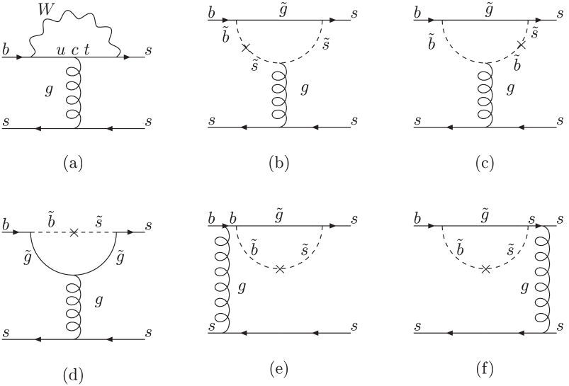
Figure 1: The SM contribution (a) and the gluino–down squark contributions (b)–(f) to the $B\to\phi K_{S}$ decay.

At the first order in the mass insertion approximation, the gluino contributions to the Wilson coefficients $C_{i,g}$ at SUSY scale $M_{S}$ are given by

$$C_{3}(M_{S}) = \frac{\sqrt{2}\alpha_{s}^{2}}{G_{F}V_{tb}V_{ts}^{*}m_{\tilde{q}}^{2}}(\delta_{LL}^{d})_{23}\left[-\frac{1}{9}B_{1}(x)-\frac{5}{9}B_{2}(x)-\frac{1}{18}P_{1}(x)-\frac{1}{2}P_{2}(x)\right],$$

$$C_{4}(M_{S}) = \frac{\sqrt{2}\alpha_{s}^{2}}{G_{F}V_{tb}V_{ts}^{*}m_{\tilde{q}}^{2}}(\delta_{LL}^{d})_{23}\left[-\frac{7}{3}B_{1}(x)+\frac{1}{3}B_{2}(x)+\frac{1}{6}P_{1}(x)+\frac{3}{2}P_{2}(x)\right],$$

$$C_{5}(M_{S}) = \frac{\sqrt{2}\alpha_{s}^{2}}{G_{F}V_{tb}V_{ts}^{*}m_{\tilde{q}}^{2}}(\delta_{LL}^{d})_{23}\left[\frac{10}{9}B_{1}(x)+\frac{1}{18}B_{2}(x)-\frac{1}{18}P_{1}(x)-\frac{1}{2}P_{2}(x)\right],$$ (47)

$$C_{6}(M_{S}) = \frac{\sqrt{2}\alpha_{s}^{2}}{G_{F}V_{tb}V_{ts}^{*}m_{\tilde{q}}^{2}}(\delta_{LL}^{d})_{23}\left[-\frac{2}{3}B_{1}(x)+\frac{7}{6}B_{2}(x)+\frac{1}{6}P_{1}(x)+\frac{3}{2}P_{2}(x)\right],$$

$$C_{g}(M_{S})\!\! = \!\!-\frac{\sqrt{2}\alpha_{s}\pi}{G_{F}V_{tb}V_{ts}^{*}m_{\tilde{q}}^{2}}\!\left[\!(\delta_{LL}^{d})_{23}\left(\frac{1}{3}M_{3}(x)\!+\!3M_{4}(x)\right)\!+\!(\delta_{LR}^{d})_{23}\frac{m_{\tilde{g}}}{m_{b}}\left(\!\frac{1}{3}M_{3}(x)\!+\!3M_{2}(x)\right)\!\right]\!,$$

and the coefficients $\tilde{C}_{i,g}$ are obtained from $C_{i,g}$ by exchanging $L\leftrightarrow R$. The functions appear in these expressions can be found in Ref.[45] and $x=m^{2}_{\tilde{g}}/m^{2}_{\tilde{q}}$. As in the case of the SM, the Wilson coefficients at low energy $C_{i,g}(\mu)$, $\mu\simeq\mathcal{O}(m_{b})$, are obtained from $C_{i,g}(M_{S})$ by using Eqs. (33) and (35).

The absolute value of the mass insertions $(\delta_{AB}^{d})_{23}$, with $A,B=(L,R)$ is constrained by the experimental results for the branching ratio of the $B\to X_{s}\gamma$ decay [45, 47]. These constraints are very weak on the $LL$ and $RR$ mass insertions and the only limits we have come from their definition, $|(\delta_{LL,RR}^{d})_{23}|<1$. The $LR$ and $RL$ mass insertions are more constrained and for instance with $m_{\tilde{g}}\simeq m_{\tilde{q}}\simeq 500$ GeV, we have $|(\delta_{LR,RL}^{d})_{23}|\raise 1.29167pt\hbox{$\;<$\kern-7.5pt\raise-4.73611pt\hbox{$\sim\;$}}1.6\times 10^{-2}$. Although the $LR(RL)$ mass insertion is constrained so severely, as can be seen from the above expression of $C_{g}(M_{S})$, it is enhanced by a large factor $m_{\tilde{g}}/m_{b}$. We will show in the following that this enhancement plays an important role to reproduce the observed large deviation between $\sin 2\beta$ and $S_{\phi K_{S}}$. We should recall that in the supersymmetry analysis of the direct CP violation in the kaon system, the same kind of enhancement by a factor $m_{\tilde{g}}/m_{s}$ makes the $LR$ and $RL$ mass insertions natural candidates to explain the experimental results of $\varepsilon^{\prime}/\varepsilon$ [46].

As shown in Eq. (20), the deviation of $S_{\phi K_{S}}$ from $\sin 2\beta$ is governed by the size of $|A^{\mathrm{SUSY}}|/|A^{\mathrm{SM}}|$. Thus we start our analysis by discussing the gluino contribution to $|A^{\mathrm{SUSY}}|/|A^{\mathrm{SM}}|$. We choose the input parameters as

$$m_{\tilde{q}}=500\mbox{GeV},\ x=1,\ q^{2}=m_{b}^{2}/2,\ \mu=2\mbox{GeV}$$ (48)

then, we obtained

$$\frac{A^{\mathrm{SUSY}}}{A^{\mathrm{SM}}}\simeq 0.13~{}(\delta_{LL}^{d})_{23}+55.4~{}(\delta_{LR}^{d})_{23}+55.4~{}(\delta_{RL}^{d})_{23}+0.13~{}(\delta_{RR}^{d})_{23}.$$ (49)

The largest theoretical uncertainty comes from the choice of $q^{2}$. We find that the smaller values of $q^{2}$ enhance the coefficients of each mass insertions and for the minimum value $q^{2}=m_{b}^{2}/4$ gives

$$\frac{A^{\mathrm{SUSY}}}{A^{SM}}\simeq 0.23~{}(\delta_{LL}^{d})_{23}+97.4~{}(\delta_{LR}^{d})_{23}+97.4~{}(\delta_{RL}^{d})_{23}+0.23~{}(\delta_{RR}^{d})_{23}.$$ (50)

Using the constraints for each mass insertions described above, we obtain the maximum contribution from the individual mass insertions by setting the remaining three mass insertions to be zero:

$$\frac{|A^{\mathrm{SUSY}}_{LL(RR)}|}{|A^{\mathrm{SM}|}}<0.23,\ \ \frac{|A^{\mathrm{SUSY}}_{LR(RL)}|}{|A^{\mathrm{SM}}|}<1.56.\ \$$ (51)

It is worth mentioning that $(\delta_{LR}^{d})_{23}$ and $(\delta_{RL}^{d})_{23}$ contribute to $S_{\phi K_{S}}$ with the same sign, unlike their contributions to $\varepsilon^{\prime}/\varepsilon$. Therefore, in SUSY model with $(\delta_{LR}^{d})_{23}\simeq(\delta_{RL}^{d})_{23}$, we will not have the usual problem of the severe cancellation between their contributions, but we will have a constrictive interference which enhances the SUSY contribution to $S_{\phi K_{S}}$.

Now let us investigate whether any one of the mass insertions can accommodate the observed large deviation between $S_{J/\psi K_{S}}$ and $S_{\phi K_{S}}$. We start with $LL$ (same for $RR$) contribution. As can be seen from Eq. (20), a choice of the strong phase $\cos\delta_{12}=\pm 1$ gives the largest deviation between $S_{\phi K_{S}}$ and $\sin 2\beta$. Using the measured central value of $\sin 2\beta$, $|(\delta_{LL}^{d})_{23}|=1$ and $\cos\delta_{12}=\pm 1$ in the CP violation master formula Eq. (18), we obtain $S_{\phi K_{S}}$ in terms of $\arg(\delta_{LL(RR)}^{d})_{23}$ as:

$$S_{\phi K_{S}}=\frac{0.73\pm 0.45\sin(\arg(\delta_{LL(RR)}^{d})_{23}+0.818)+0.051\sin(2\arg(\delta_{LL(RR)}^{d})_{23}+0.818)}{1.05\pm 0.45\cos(\arg(\delta_{LL(RR)}^{d})_{23})}$$ (52)

Then the minimum value of $S_{\phi K_{S}}$ is obtained by $\sin(\arg(\delta_{LL(RR)}^{d})_{23})=\mp 0.97$ as

$$S_{\phi K_{S}}=0.35.$$ (53)

We find that if the experimental value for $S_{\phi K_{S}}$ remains as small as the current central value, the SUSY models with $LL$ or $RR$ mass insertion can not provide an explanation for that.

Next, we show that on the contrary, the $(\delta_{LR(RL)}^{d})_{23}$ contribution can deviate $S_{\phi K_{S}}$ from $\sin 2\beta$ much more significantly. For $|(\delta_{LR(RL)}^{d})_{23}|=0.01$ and $\cos\delta_{12}=\pm 1$, the mixing CP asymmetry is expressed as

$$S_{\phi K_{S}}=\frac{0.73\pm 1.95\sin(\arg(\delta_{LR(RL)}^{d})_{23}+0.818)+0.95\sin(2\arg(\delta_{LR(RL)}^{d})_{23}+0.818)}{1.95\pm 1.95\cos(\arg(\delta_{LR(RL)}^{d})_{23})}.$$ (54)

and the minimum value is obtained with $\sin(\arg(\delta_{LR(RL)}^{d})_{23})=(\mp 0.075,\ \mp 0.63)$ as

$$S_{\phi K_{S}}=-1.$$ (55)

In Fig.2, we present plots for the phase of $(\delta_{LL(RR)}^{d})_{23}$ and $(\delta_{LR(RL)}^{d})_{23}$ versus the mixing CP asymmetry $S_{\phi K_{S}}$ for $\cos\delta_{12}=1$. We choose the three values of the magnitude of these mass insertions within the bounds from the experimental limits in particular, from $B\to X_{s}\gamma$. Each plot shows a contribution from an individual mass insertion by setting the other three to be zero. As can be seen from these plots, the $LR$ (same for $RL$) gives the largest contribution to $S_{\phi K_{S}}$. In order to have a sizable effect from the $LL$ or $RR$, the magnitude of $(\delta_{LL(RR)}^{d})_{23}$ has to be of order one and furthermore, the imaginary part needs to be as large as the real part. In any case, it is very difficult to give negative value of $S_{\phi K_{S}}$ from $(\delta_{LL}^{d})_{23}$ or $(\delta_{RR}^{d})_{23}$ mass insertion. On the contrary, even if we reduce the magnitude of $(\delta_{LR}^{d})_{23}$ to the half of its maximum value, $S_{\phi K_{S}}$ can still reach to a negative value. We also find that in the case of $|(\delta^{d}_{LR(RL)})_{23}|=0.01$, the minimum value of $S_{\phi K_{S}}$ can be achieved without large imaginary part. Actually, we should notify that smaller values of the ratio $x=m_{\tilde{g}}^{2}/m_{\tilde{q}}^{2}$ can lead to large $LL$ and $RR$ contributions to $S_{\phi K_{S}}$. However, the negative value of $S_{\phi K_{S}}$ can be only achieved by the light gluino mass around the current experimental limit and very heavy (order of TeV) squark mass.

\psfrag{(a)}[r][r][0.3]{(a)}\psfrag{(c)}[r][r][0.3]{(b)}\psfrag{s}[r][l][0.3]{$S_{\phi K_{S}}$}\psfrag{1ll}[l][l][0.2]{\large$|(\delta_{LL(RR)}^{d})_{23}|=0.1$}\psfrag{2ll}[l][l][0.2]{\large$|(\delta_{LL(RR)}^{d})_{23}|=0.5$}\psfrag{3ll}[l][l][0.2]{\large$|(\delta_{LL(RR)}^{d})_{23}|=1$}\psfrag{1lr}[l][l][0.2]{\large$|(\delta_{LR(RL)}^{d})_{23}|=0.001$}\psfrag{2lr}[l][l][0.2]{\large$|(\delta_{LR(RL)}^{d})_{23}|=0.005$}\psfrag{3lr}[l][l][0.2]{\large$|(\delta_{LR(RL)}^{d})_{23}|=0.01$}\psfrag{ll}[l][l][0.35]{$\arg[(\delta_{LL(RR)}^{d})_{23}]$}\psfrag{lr}[l][l][0.35]{$\arg[(\delta_{LR(RL)}^{d})_{23}]$}\includegraphics[width=284.52756pt,height=142.26378pt,keepaspectratio]{figure2.eps}

Figure 2: The mixing CP asymmetry as function of $\arg[(\delta_{AB}^{d})_{23}]$ for three values of the $|(\delta_{AB}^{d})_{23}|$ where $AB=LL(RR)\mbox{(a)},\ LR(RL)\mbox{(b)}$. The strong phase $\delta_{12}$ is fixed at $\cos\delta_{12}=1$.

So far, we have only considered the cases where the strong phase $\delta_{12}$ is given by $\cos\delta_{12}=\pm 1$ so that the direct CP asymmetry $C_{\phi K_{S}}$ was identically zero. However, since the correlation between $S_{\phi K_{S}}$ and $C_{\phi K_{S}}$ would be very useful to give some constrains on SUSY parameters, here we include arbitrary strong phases and demonstrate an example of $S_{\phi K_{S}}-C_{\phi K_{S}}$ correlation. By using the expanded formulae for $S_{\phi K_{S}}$ and $C_{\phi K_{S}}$ in Eqs. (20) and (21), we find that for any value of $\delta_{12}$, the plot of $S_{\phi K_{S}}$ versus $C_{\phi K_{S}}$ becomes an ellipse with its size proportional to $\sin\theta_{SUSY}$:

$$\frac{(S_{\phi K_{S}}-\sin 2\beta)^{2}}{\cos^{2}2\beta\left(2\sin\theta_{SUSY}\frac{|A^{\mathrm{SUSY}}|}{|A^{\mathrm{SM}}|}\right)^{2}}+\frac{C_{\phi K_{S}}^{2}}{\left(2\sin\theta_{SUSY}\frac{|A^{\mathrm{SUSY}}|}{|A^{\mathrm{SM}}|}\right)^{2}}=1$$ (56)

In Fig.3, we depict an example of the plot with $|A^{\mathrm{SUSY}}|/|A^{\mathrm{SM}}|\simeq 0.5$ and $\theta_{SUSY}=(\pi/20,\pi/4,\pi/2,3\pi/5,4\pi/3)$. Since we used the full formulae in Eqs. (18) and (19) to create this figure, different $\theta_{SUSY}$ does not give precisely rescaled ellipses. Nevertheless we can see the qualitative feature. The strong phase $\delta_{12}=0$ corresponds to the point at the right most tip of the ellipse. As $\delta_{12}$ increases, it runs anti-clockwise and finishes a round when $\delta_{12}=2\pi$. Note that with $|A^{\mathrm{SUSY}}|/|A^{\mathrm{SM}}|\simeq 0.5$, a typical branching ratio is about $10\times 10^{-6}$, which is within the range of experimental value. As experimental errors will be reduced, this kind of plot would provide very interesting constraints on SUSY parameters.

\psfrag{s}[r][l][1]{$S_{\phi K_{S}}$}\psfrag{c}[r][l][1]{$C_{\phi K_{S}}$}\psfrag{miss}[r][l][0.7]{$\pi/2$}\includegraphics[width=284.52756pt,height=284.52756pt,keepaspectratio]{figure3.eps}

Figure 3: The mixing CP asymmetry $S_{\phi K_{S}}$ versus the direct CP symmetry $C_{\phi K_{S}}$ for strong phase $\delta_{12}\in[0,2\pi]$ and five representative values of $\theta_{SUSY}=(\pi/20,\pi/4,\pi/2,3\pi/5,4\pi/3)$.

5 CP asymmetry $S_{\phi K_{S}}$ in explicit SUSY models

In this section, we study the CP asymmetry of the $B\to\phi K_{S}$ in some specific SUSY models. We consider the minimal supersymmetric standard model (MSSM) (where minimal number of superfields is introduced and $R$ parity is conserved) with the following soft SUSY breaking terms

$$V_{SB} = m_{0\alpha}^{2}\phi_{\alpha}^{*}\phi_{\alpha}+\epsilon_{ab}(A^{u}_{ij}Y^{u}_{ij}H_{2}^{b}\tilde{q}_{L_{i}}^{a}\tilde{u}^{*}_{R_{j}}+A^{d}_{ij}Y^{d}_{ij}H_{1}^{a}\tilde{q}_{L_{i}}^{b}\tilde{d}^{*}_{R_{j}}+A^{l}_{ij}Y^{l}_{ij}H_{1}^{a}\tilde{l}_{L_{i}}^{b}\tilde{e}^{*}_{R_{j}}$$ (57)

$$- B\mu H_{1}^{a}H_{2}^{b}+\mathrm{H.c.})-\frac{1}{2}(m_{3}\bar{\tilde{g}}\tilde{g}+m_{2}\overline{\widetilde{W^{a}}}\widetilde{W}^{a}+m_{1}\bar{\tilde{B}}\tilde{B})\;,$$

where $i,j$ are family indices, $a,b$ are $SU(2)$ indices, $\epsilon_{ab}$ is the $2\times 2$ fully antisymmetric tensor, with $\epsilon_{12}=1$, and $\phi_{\alpha}$ denotes all the scalar fields of the theory. We start with minimal supergravity model and then we consider general SUSY models with non–universal soft breaking terms. We also discuss the impact of the type of Yukawa couplings on the prediction of the later model.

5.1 minimal supergravity model

In a minimal supergravity framework, the soft SUSY breaking parameters are universal at GUT scale, and we can write

$$m_{0\alpha}^{2}=m_{0}^{2}\;,\quad m_{i}=m_{1/2}\;,\quad A^{\alpha}_{ij}=A_{0}e^{i\phi_{A}}\;.$$ (58)

In this model, there are only two physical phases: $\phi_{A}=\arg(A^{*}m_{1/2})$ and $\phi_{\mu}=\arg(\mu m_{1/2})$. In order to have EDM values below the experimental bounds, and without forcing the SUSY masses to be unnaturally heavy, the phases $\phi_{A}$ and $\phi_{\mu}$ must be at most of order $10^{-1}$ and $10^{-2}$, respectively [22].

It is clear that this class of models, where the SUSY phases are constrained to be very small and the Yukawa couplings are the main source of the flavour structure, can not generate sizable contributions to the CP violating parameters. And it is indeed the case for $S_{\phi K_{S}}$. We find that it is impossible to have a large deviation between $S_{\phi K_{S}}$ and $\sin 2\beta$ within the minimal supergravity framework.

In fact, we find that even if we ignore the bounds from the EDM, and allow large values for SUSY phases, $\phi_{A,\mu}\simeq\pi/2$, still the SUSY contribution to $S_{\phi K_{S}}$ is negligible. The suppression is mainly due to the universality assumption of the soft breaking terms. For instance, with $m_{1/2}\simeq m_{0}\simeq A_{0}\simeq 200$ GeV we find the following values of the relevant mass insertions:

$$(\delta^{d}_{LL})_{23} \simeq 0.009+i~{}0.001,$$ (59)

$$(\delta^{d}_{RR})_{23} \simeq -2.1\times 10^{-7}-i~{}2.5\times 10^{-8},$$ (60)

$$(\delta^{d}_{LR})_{23} \simeq -2.5\times 10^{-5}-i~{}1.9\times 10^{-5}.$$ (61)

Clearly these values are much smaller than the corresponding values mentioned in the previous section and it gives negligible contributions to the CP asymmetry $S_{\phi K_{S}}$. Indeed, we find that the total $S_{\phi K_{S}}$ in this example is given by $S_{\phi K_{S}}=0.729$, which is about the value of $\sin 2\beta$.

5.2 SUSY models with non–universal soft terms

Now we consider SUSY models with non–universal soft terms. In particular, we focus on the models with non–universal $A$–terms in order to enhance the values of $(\delta_{LR}^{d})_{23}$ and $(\delta_{RL}^{d})_{23}$, which may give the dominant contributions to the CP asymmetry $S_{\phi K_{S}}$. However, non–observation of EDMs leads to restrictive constraints on the non–degenerate $A$–terms and only certain patterns of flavour are allowed, such as the Yukawa and $A$–terms are Hermitian [23], or the $A$–terms are factorisable, i.e., $(Y^{A})_{ij}=A.Y$ or $Y.A$ [46]. In the case of factorisation, the mass insertion $(\delta^{d}_{LR})_{11}$ is suppressed by the ratio $m_{d}/m_{\tilde{q}}$. Here we will consider this scenario with the following trilinear structure:

$$A=m_{0}\left(\begin{array}[]{ccc}a&a&a\\ b&b&b\\ c&c&c\end{array}\right)\;.$$ (62)

As pointed out in Ref.[24], in the case of non–universal soft breaking terms, the type of the Yukawa couplings (hierarchical or nearly democratic) plays an important role and has significant impact on the predictions of these models. If we consider the standard example of hierarchical quark Yukawa matrices,

$$Y_{u} = \frac{1}{v\sin\beta}\mathrm{diag}\left(m_{u},m_{c},m_{t}\right),$$

$$Y_{d} = \frac{1}{v\cos\beta}K.\mathrm{diag}\left(m_{u},m_{c},m_{t}\right).K^{+},$$ (63)

where $K$ is the CKM matrix, the relevant $LR$ mass insertion is given by

$$(\delta_{LR}^{d})_{23}\simeq\frac{v\cos\beta}{m_{\tilde{q}^{2}}}\left(K^{+}~{}Y^{A}_{d}~{}K\right)_{23}$$ (64)

where $(Y_{d}^{A})_{ij}=Y^{d}_{ij}A^{d}_{ij}$. It is clear that the dominant contribution to this mass insertion is given by the term $K_{22}(Y_{d}^{A})_{23}K_{33}^{+}$ which is still suppressed by the small entry of $Y^{d}_{23}$. The non–universality of the squarks can enhance the $LL$ and $RR$ mass insertions, however this non–universality is severely constrained by the experimental measurements of $\Delta M_{K}$ and $\varepsilon_{K}$. Therefore, with the hierarchical Yukawa couplings we find that the typical values of the relevant mass insertions are at least two order of magnitude below the required values so that contributions to split the CP asymmetries $S_{J/\psi K_{S}}$ from $S_{\phi K_{S}}$ are again small.

Now we consider the same SUSY model but with converting the above hierarchical Yukawa matrices to democratic ones, which can be obtained by a unitary transformation. As emphasised in Ref.[24] that these new Yukawa textures (and their diagonalising matrices $S^{u,d}_{L,R}$) have large mixing, which has important consequences in the SUSY results. Thus, the element $(Y_{d}^{A})_{23}$ has no suppression factor as before and the magnitude of $(\delta_{LR}^{d})_{23}$ can be of the desired order. As a numerical example, for $m_{0}=m_{1/2}=200$ GeV, (i.e., $m_{\tilde{q}}\simeq m_{g}\simeq 500$ GeV) and assuming that $|A_{ij}|\in[m_{0},4m_{0}]$ while the phases of the $A$–terms are chosen such that the bound of the EDMs are satisfied, we find that it is quite natural to obtain the following values of the mass insertion $(\delta_{LR}^{d})_{23}$: $|(\delta_{LR}^{d})_{23}|\simeq 0.005$ and $\mathrm{Arg}[(\delta_{LR}^{d})_{23}]\simeq 1.2$ which leads to $S_{\phi K_{S}}\simeq-0.2$.

6 Conclusions

In this paper, we have studied the supersymmetric contributions to the CP asymmetry of $B\to\phi K_{S}$ process. Using the mass insertion approximation method, we have derived model independent limits for the mixing CP asymmetry $S_{\phi K_{S}}$. We found that the $LR$ or $RL$ mass insertion gives the largest contribution to $S_{\phi K_{S}}$, while the $LL$ or $RR$ contribution is small. Thus, we conclude that if the deviation between $S_{\phi K_{S}}$ and $S_{J/\psi K_{S}}$ observed by the B–factory experiments (Belle and BaBar) remains as large as its present central value, the SUSY models with large ($\sim 10^{-3}$) $LR(RL)$ mass insertions will be an interesting candidate to explain this phenomena.

The Belle collaboration observed non–vanishing direct CP asymmetry $C_{\phi K_{S}}$ which can be obtained only by simultaneous non–vanishing strong phase and SUSY CP violating phase. Thus, we studied the impact of the strong phase in our results for $S_{\phi K_{S}}$. We provided an example of a plot to show a correlation between $S_{\phi K_{S}}$ and $C_{\phi K_{S}}$. Our result will be useful to give constraints on some SUSY parameters as experimental errors will be reduced.

We also applied our results to the minimal supergravity model and SUSY models with non–universal soft terms with two types of Yukawa couplings, hierarchal and nearly democratic Yukawa textures. We showed that only in SUSY models with large Yukawa mixing, SUSY contributions could be enhanced and reach the desired values to give significant contributions to the CP asymmetry $S_{\phi K_{S}}$. This result motivates the interest in SUSY models with non–universal soft terms and also shed the light on the type of the Yukawa flavour structure.

Note added in proof

We have found an error in our program and the $RR$ contribution is enhanced by one order of magnitude in this revised version. As a result, we agree with the results in Refs.  [48, 49].

References

- [1] M. Kobayashi and T. Maskawa, Prog. Theor. Phys. 49 (1973) 652.
- [2] B. Aubert et al. [BABAR Collaboration], Phys. Rev. Lett. 89 (2002) 201802 [arXiv:hep-ex/0207042].
- [3] K. Abe et al. [Belle Collaboration], arXiv:hep-ex/0207098.
- [4] E. Gabrielli and S. Khalil, arXiv:hep-ph/0207288 to be published in Phys. Rev. D.
- [5] Y. Grossman and M. P. Worah, Phys. Lett. B 395 (1997) 241 [arXiv:hep-ph/9612269].
- [6] D. London and A. Soni, Phys. Lett. B 407 (1997) 61 [arXiv:hep-ph/9704277].
- [7] Y. Grossman, G. Isidori and M. P. Worah, Phys. Rev. D 58 (1998) 057504 [arXiv:hep-ph/9708305].
- [8] Y. Nir, arXiv:hep-ph/0208080.
- [9] B. Aubert et al. [BABAR Collaboration], arXiv:hep-ex/0207070.
- [10] M. Tanimoto, K. Hirayama, T. Shinmoto and K. Senba, Z. Phys. C 48 (1990) 99.
- [11] E. Lunghi and D. Wyler, Phys. Lett. B 521 (2001) 320 [arXiv:hep-ph/0109149].
- [12] T. Moroi, Phys. Lett. B 493 (2000) 366 [arXiv:hep-ph/0007328].
- [13] X. G. He, J. P. Ma and C. Y. Wu, Phys. Rev. D 63 (2001) 094004 [arXiv:hep-ph/0008159].
- [14] D. Chang, A. Masiero and H. Murayama, arXiv:hep-ph/0205111.
- [15] M. B. Causse, arXiv:hep-ph/0207070.
- [16] G. Hiller, Phys. Rev. D 66 (2002) 071502 [arXiv:hep-ph/0207356].
- [17] M. Ciuchini and L. Silvestrini, Phys. Rev. Lett. 89 (2002) 231802 [arXiv:hep-ph/0208087].
- [18] M. Raidal, Phys. Rev. Lett. 89 (2002) 231803 [arXiv:hep-ph/0208091].
- [19] A. Datta, Phys. Rev. D 66 (2002) 071702 [arXiv:hep-ph/0208016].
- [20] J. P. Lee and K. Y. Lee, arXiv:hep-ph/0209290.
- [21] B. Dutta, C. S. Kim and S. Oh, arXiv:hep-ph/0208226.
- [22] S. Abel, S. Khalil and O. Lebedev, Nucl. Phys. B 606 (2001) 151 [arXiv:hep-ph/0103320], and refernce therein.
- [23] S. Abel, D. Bailin, S. Khalil and O. Lebedev, Phys. Lett. B 504 (2001) 241 [arXiv:hep-ph/0012145]; S. Khalil, arXiv:hep-ph/0202204.
- [24] S. Abel, G. C. Branco and S. Khalil, arXiv:hep-ph/0211333.
- [25] E. Gabrielli, S. Khalil and E. Torrente-Lujan, Nucl. Phys. B 594 (2001) 3 [arXiv:hep-ph/0005303]; E. Gabrielli and S. Khalil, Phys. Lett. B 530 (2002) 133 [arXiv:hep-ph/0201049].
- [26] A. L. Kagan, Phys. Rev. D 51 (1995) 6196 [arXiv:hep-ph/9409215]; arXiv:hep-ph/9806266; Lecture at the SLAC Summer Institute, August 2002, http://www.slac.stanford.edu/gen/meeting/ssi/2002/kagan1.html#lecture2; A. L. Kagan and M. Neubert, Phys. Rev. D 58 (1998) 094012 [arXiv:hep-ph/9803368]
- [27] M. Ciuchini, E. Gabrielli and G. F. Giudice, Phys. Lett. B 388 (1996) 353 [Erratum-ibid. B 393 (1997) 489] [arXiv:hep-ph/9604438].
- [28] A. Ali and C. Greub, Phys. Rev. D 57 (1998) 2996 [arXiv:hep-ph/9707251].
- [29] I. I. Bigi and A. I. Sanda, Cambridge Monogr. Part. Phys. Nucl. Phys. Cosmol. 9 (2000) 1.
- [30] Y. Grossman, Y. Nir and M. P. Worah, Phys. Lett. B 407 (1997) 307 [arXiv:hep-ph/9704287].
- [31] Y. Nir, arXiv:hep-ph/9810520.
- [32] M. Gronau, Phys. Lett. B 300 (1993) 163 [arXiv:hep-ph/9209279].
- [33] K. F. Chen [BELLE Collaboration], talk given at 31st International Conference On High Energy Physics (ICHEP 2002) 24-31 Jul 2002, Amsterdam, The Netherlands
- [34] B. Aubert et al. [BABAR Collaboration], Phys. Rev. Lett. 87 (2001) 151801 [arXiv:hep-ex/0105001].
- [35] A. J. Buras and L. Silvestrini, Nucl. Phys. B 548 (1999) 293 [arXiv:hep-ph/9806278].
- [36] H. Y. Cheng, H. n. Li and K. C. Yang, Phys. Rev. D 60 (1999) 094005 [arXiv:hep-ph/9902239]; Y. H. Chen, H. Y. Cheng, B. Tseng and K. C. Yang, Phys. Rev. D 60 (1999) 094014 [arXiv:hep-ph/9903453].
- [37] Y. Y. Keum, H. n. Li and A. I. Sanda, Phys. Lett. B 504 (2001) 6 [arXiv:hep-ph/0004004]; Phys. Rev. D 63 (2001) 054008 [arXiv:hep-ph/0004173].
- [38] M. Beneke, G. Buchalla, M. Neubert and C. T. Sachrajda, Phys. Rev. Lett. 83 (1999) 1914 [arXiv:hep-ph/9905312]; Nucl. Phys. B 591 (2000) 313 [arXiv:hep-ph/0006124]; Nucl. Phys. B 606 (2001) 245 [arXiv:hep-ph/0104110].
- [39] S. Mishima, Phys. Lett. B 521 (2001) 252 [arXiv:hep-ph/0107206].
- [40] C. H. Chen, Y. Y. Keum and H. n. Li, Phys. Rev. D 64 (2001) 112002 [arXiv:hep-ph/0107165].
- [41] H. Y. Cheng and K. C. Yang, Phys. Rev. D 64 (2001) 074004 [arXiv:hep-ph/0012152].
- [42] A. J. Buras, arXiv:hep-ph/9806471.
- [43] A. Ali, G. Kramer and C. D. Lu, Phys. Rev. D 58 (1998) 094009 [arXiv:hep-ph/9804363].
- [44] P. Ball, JHEP 9809 (1998) 005 [arXiv:hep-ph/9802394].
- [45] F. Gabbiani, E. Gabrielli, A. Masiero and L. Silvestrini, Nucl. Phys. B 477 (1996) 321 [arXiv:hep-ph/9604387].
- [46] S. Khalil, T. Kobayashi and O. Vives, Nucl. Phys. B 580 (2000) 275 [arXiv:hep-ph/0003086]; S. Khalil and T. Kobayashi, Phys. Lett. B 460 (1999) 341 [arXiv:hep-ph/9906374]; S. Khalil, T. Kobayashi and A. Masiero, Phys. Rev. D 60 (1999) 075003 [arXiv:hep-ph/9903544].
- [47] M. B. Causse and J. Orloff, Eur. Phys. J. C 23 (2002) 749 [arXiv:hep-ph/0012113].
- [48] R. Harnik, D. T. Larson, H. Murayama and A. Pierce, arXiv:hep-ph/0212180.
- [49] M. Ciuchini, E. Franco, A. Masiero and L. Silvestrini, arXiv:hep-ph/0212397.