Abstract

The status of the evaluation of the MSSM Higgs sector is reviewed. The phenomenological impact of recently obtained corrections is discussed. In particular it is shown that the upper bound on $m_{h}$ within the MSSM is shifted upwards. Consequently, lower limits on $\tan\beta\hskip 2.84526pt$ obtained by confronting the upper bound as function of $\tan\beta$ with the lower bound on $m_{h}$ from Higgs searches are significantly weakened. Furthermore, the region in the $M_{A}$–$\tan\beta$-plane where the coupling of the lightest Higgs boson to down-type fermions is suppressed is modified. The presently not calculated higher-order corrections to the Higgs-boson mass matrix are estimated to shift the mass of the lightest Higgs boson by up to $3\,\,\mathrm{GeV}$.

1 Introduction

A crucial prediction of the Minimal Supersymmetric Standard Model (MSSM) [1] is the existence of at least one light Higgs boson. The search for this particle is one of the main goals at the present and the next generation of colliders. Direct searches at LEP have already ruled out a considerable fraction of the MSSM parameter space, and the forthcoming high-energy experiments at the Tevatron, the LHC and a future Linear Collider (LC) will either discover a light Higgs boson or rule out the MSSM as a viable theory for physics at the weak scale. Furthermore, if one or more Higgs bosons are discovered, their masses and couplings will be determined with high accuracy at a future LC. Thus, a precise knowledge of the dependence of the masses and mixing angles of the MSSM Higgs sector on the relevant supersymmetric parameters is of utmost importance to reliably compare the predictions of the MSSM with the (present and future) experimental results.

We recall that the Higgs sector of the MSSM [2] consists of two neutral ${\cal CP}$-even Higgs bosons, $h$ and $H$ ($m_{h}<m_{H}$), the ${\cal CP}$-odd $A$ boson, and two charged Higgs bosons, $H^{\pm}$. At the tree-level, $m_{h,{\rm tree}}$ and $m_{H,{\rm tree}}$ can be calculated in terms of the Standard Model (SM) gauge couplings and two additional MSSM parameters, conventionally chosen as $M_{A}$ and $\tan\beta$, the ratio of the two vacuum expectation values ($\tan\beta=v_{2}/v_{1}$). The two masses are obtained by rotating the neutral ${\cal CP}$-even Higgs boson mass matrix with an angle $\alpha$,

$$M_{\rm Higgs}^{2,{\rm tree}} = \left(\begin{array}[]{cc}M_{A}^{2}\sin^{2}\beta\hskip 2.84526pt+M_{Z}^{2}\cos^{2}\beta&-(M_{A}^{2}+M_{Z}^{2})\sin\beta\hskip 2.84526pt\cos\beta\\ -(M_{A}^{2}+M_{Z}^{2})\sin\beta\hskip 2.84526pt\cos\beta&M_{A}^{2}\cos^{2}\beta\hskip 2.84526pt+M_{Z}^{2}\sin^{2}\beta\end{array}\right),$$ (3)

with $\alpha$ satisfying

$$\tan 2\alpha=\tan 2\beta\frac{M_{A}^{2}+M_{Z}^{2}}{M_{A}^{2}-M_{Z}^{2}},\quad-\frac{\pi}{2}<\alpha<0.$$ (4)

In the Feynman diagrammatic (FD) approach the higher-order corrected Higgs boson masses are derived by finding the poles of the $h,H$-propagator matrix whose inverse is given by

$$\left(\Delta_{\rm Higgs}\right)^{-1}=-i\left(\begin{array}[]{cc}p^{2}-m_{H,{\rm tree}}^{2}+\hat{\Sigma}_{HH}(p^{2})&\hat{\Sigma}_{hH}(p^{2})\\ \hat{\Sigma}_{hH}(p^{2})&p^{2}-m_{h,{\rm tree}}^{2}+\hat{\Sigma}_{hh}(p^{2})\end{array}\right),$$ (5)

where the $\hat{\Sigma}(p^{2})$ denote the renormalized Higgs-boson self-energies, $p$ being the momentum flowing on the external legs. Determining the poles of the matrix $\Delta_{\rm Higgs}$ in eq. (5) is equivalent to solving the equation

$$\left[p^{2}-m_{h,{\rm tree}}^{2}+\hat{\Sigma}_{hh}(p^{2})\right]\left[p^{2}-m_{H,{\rm tree}}^{2}+\hat{\Sigma}_{HH}(p^{2})\right]-\left[\hat{\Sigma}_{hH}(p^{2})\right]^{2}=0\,.$$ (6)

The status of the available results for the self-energy contributions to eq. (5) can be summarized as follows. For the one-loop part, the complete result within the MSSM is known [3, 4, 5, 6]. The by far dominant one-loop contribution is the ${\cal O}(\alpha_{t})$ term due to top and stop loops ($\alpha_{t}\equiv h_{t}^{2}/(4\pi)$, $h_{t}$ being the superpotential top coupling). Concerning the two-loop effects, their computation is quite advanced and it has now reached a stage such that all the presumably dominant contributions are known. They include the strong corrections, usually indicated as ${\cal O}(\alpha_{t}\alpha_{s})$, and Yukawa corrections, ${\cal O}(\alpha_{t}^{2})$, to the dominant one-loop ${\cal O}(\alpha_{t})$ term, as well as the strong corrections to the bottom/sbottom one-loop ${\cal O}(\alpha_{b})$ term ($\alpha_{b}\equiv h_{b}^{2}/(4\pi)$), i.e. the ${\cal O}(\alpha_{b}\alpha_{s})$ contribution. The latter can be relevant for large values of $\tan\beta\hskip 2.84526pt$. Presently, the ${\cal O}(\alpha_{t}\alpha_{s})$ [7, 8, 9, 10, 11], ${\cal O}(\alpha_{t}^{2})$ [7, 12, 13] and the ${\cal O}(\alpha_{b}\alpha_{s})$ [14] contributions to the self-energies are known for vanishing external momenta. In the (s)bottom corrections the all-order resummation of the $\tan\beta\hskip 2.84526pt$-enhanced terms, ${\cal O}(\alpha_{b}(\alpha_{s}\tan\beta)^{n})$, is also performed [15, 16].

In this paper we are going to present, in view of the recent achievements obtained in the knowledge of the two-loop corrections, updated results for various quantities of physical interest. In our analysis we employ the latest version of the Fortran code FeynHiggs [17, 18], namely FeynHiggs1.3, that evaluates the MSSM neutral ${\cal CP}$-even Higgs sector masses and the mixing angle.

The paper is organized as follows: in Section 2 we give a brief summary of recent theoretical improvements in the MSSM Higgs sector and describe the corresponding modifications in the code FeynHiggs in order to comprise all existing higher-order results. We compare the results for $m_{h}$ obtained employing different approximations in the treatment of the two-loop corrections. In Section 3 we present the results for the phenomenological implications of our improved knowledge of the two-loop contributions to the Higgs boson self-energies. Section 4 contains a discussion of the presently unknown contributions in the prediction for the ${\cal CP}$-even Higgs-boson masses of the MSSM, and an estimate of their possible numerical importance is given. Finally, in Section 5 we draw our conclusions.

2 Recent improvements in the MSSM Higgs sector and implementation in FeynHiggs

In order to discuss the impact of recent improvements in the MSSM Higgs sector we will make use of the program FeynHiggs [17, 18], which is a Fortran code for the evaluation of the neutral ${\cal CP}$-even Higgs sector of the MSSM including higher-order corrections to the renormalized Higgs boson self-energies. The original release included the well known full one-loop corrections [3, 4, 5, 6], the two-loop leading, momentum-independent, ${\cal O}(\alpha_{t}\alpha_{s})$ correction in the top/stop sector [8, 9, 11] as well as the two-loop leading logarithmic corrections at ${\cal O}(\alpha_{t}^{2})$ [19, 20]. By two-loop momentum-independent corrections here and hereafter we mean the two-loop contributions to Higgs boson self-energies evaluated at zero external momenta. At the one-loop level, the momentum-independent contributions are the dominant part of the self-energy corrections, that, in principle, should be evaluated at external momenta equal to the poles of the $h,H$-propagator matrix, eq. (5).

The new version of FeynHiggs  contains a modification in the one-loop part due to a different renormalization prescription employed and includes also several new corrections to the Higgs boson self-energies that have recently been calculated. These changes are described in the following subsections.

With the implementation of the latest results obtained in the MSSM Higgs sector, FeynHiggs comprises all available higher-order corrections and thus allows the presently most precise prediction of the masses of the ${\cal CP}$-even Higgs bosons and the corresponding mixing angle. The latest version of FeynHiggs, FeynHiggs1.3, can be obtained from www.feynhiggs.de.

2.1 Hybrid renormalization scheme at the one-loop level

FeynHiggs is based on the FD approach with on-shell renormalization conditions [9]. This means in particular that all the masses in the FD result are the physical ones, i.e. they correspond to physical observables. Since eq. (6) is solved iteratively, the result for $m_{h}$ and $m_{H}$ contains a dependence on the field-renormalization constants of $h$ and $H$, which is formally of higher order. Accordingly, there is some freedom in choosing appropriate renormalization conditions for fixing the field-renormalization constants (this can also be interpreted as affecting the renormalization of $\tan\beta$). Different renormalization conditions have been considered in the literature, e.g. ($\hat{\Sigma}^{\prime}$ denotes the derivative with respect to the external momentum squared):

1. on-shell renormalization for $\hat{\Sigma}_{Z},\hat{\Sigma}_{A},\hat{\Sigma}^{\prime}_{A},\hat{\Sigma}_{AZ}$, and $\delta v_{1}/v_{1}=\delta v_{2}/v_{2}$ [6]

2. on-shell renormalization for $\hat{\Sigma}_{Z},\hat{\Sigma}_{A},\hat{\Sigma}_{AZ}$, and $\delta v_{i}=\delta v_{i,{\rm div}},i=1,2$ [5, 21]

3. on-shell renormalization for $\hat{\Sigma}_{Z},\hat{\Sigma}_{A}$ , $\overline{\rm{DR}}$ renormalization (employing dimensional reduction [22]) for $\delta Z_{h},\delta Z_{H}$ and $\tan\beta$ [18].

Versions of FeynHiggs previous than the 1.2 release were based on type-1 renormalization conditions, thus requiring the derivative of the $A$ boson self-energy. The latest versions employ instead the hybrid $\overline{\rm{DR}}$/on-shell type 3 conditions[18]. The choice of a $\overline{\rm{DR}}$ definition for $\delta Z_{h},\delta Z_{H}$ and $\tan\beta$ requires to specify a renormalization scale $Q^{2}$ at which these parameters are defined. This scale is set to $m_{t}^{2}$ in FeynHiggs, but can be changed by the user. These new renormalization conditions lead to a more stable behavior around thresholds, e.g. $M_{A}=2\,m_{t}$, and avoid unphysically large contributions in certain regions of the MSSM parameter space (a detailed discussion can be found in Ref. [23]; see also Ref. [24]).

2.2 Two-loop ${\cal O}(\alpha_{t}^{2})$ corrections

In the previous version of FeynHiggs the two-loop ${\cal O}(\alpha_{t}^{2})$ corrections were implemented in a simplified form, taken over from the result of [19, 20], obtained with the renormalization group (RG) method. The latter result included the two-loop leading logarithmic corrections, proportional to the square of $t\equiv\log\,(M_{\rm SUSY}^{2}/m_{t}^{2})$ (where $M_{\rm SUSY}$ is a common scale for the soft SUSY-breaking parameters), while the next-to-leading logarithmic terms, linear in $t$, were not totally accounted for.

Recently, the two-loop ${\cal O}(\alpha_{t}^{2})$ corrections in the limit of zero external momentum became available, first only for the lightest eigenvalue, $m_{h}$, and in the limit $M_{A}\gg M_{Z}$ [12], then for all the entries of the Higgs propagator matrix for arbitrary values of $M_{A}$ [13]. They were obtained in the effective-potential approach, that allows to construct the Higgs boson self-energies, at zero external momenta, by taking the relevant derivatives of the field-dependent potential. In this procedure it is important, in order to make contact with the physical $M_{A}$, to compute the effective potential as a function of both ${\cal CP}$-even and ${\cal CP}$-odd fields, as emphasized in Ref. [11]. In the evaluation of the ${\cal O}(\alpha_{t}^{2})$ corrections, the specification of a renormalization prescription for the Higgs mixing parameter $\mu$ is also required and it has been chosen as $\overline{\rm{DR}}$. In FeynHiggs1.3, which includes the complete two-loop ${\cal O}(\alpha_{t}^{2})$ corrections, the corresponding renormalization scale is fixed to be the same as for $\delta Z_{h},\delta Z_{H}$ and $\tan\beta$.

Figure 1: Two-loop corrected $m_{h}$ as a function of $X_{t}$ in various steps of approximation. The relevant MSSM parameters are chosen as $\tan\beta=3\,,\,m_{t}^{\rm pole}=174.3\,\,\mathrm{GeV}$, $M_{\tilde{t}_{L}}=M_{\tilde{t}_{R}}=M_{A}=\mu=1\,\,\mathrm{TeV}$ and $m_{\tilde{g}}=800\,\,\mathrm{GeV}$. The meaning of the different curves is explained in the text.

The availability of the complete result for the momentum-independent part of the ${\cal O}(\alpha_{t}^{2})$ corrections allows us to judge the quality of results that incorporate only the logarithmic contributions. In Fig. 1 we plot the two-loop corrected $m_{h}$ as a function of the stop mixing parameter, $X_{t}\equiv A_{t}-\mu/\tan\beta$, where $A_{t}$ denotes the trilinear soft SUSY breaking Higgs–stop coupling. We use the following convention for the stop mass matrix,

$${\cal M}^{2}_{\tilde{t}}=\left(\begin{array}[]{cc}M_{\tilde{t}_{L}}^{2}+m_{t}^{2}+\cos 2\beta\hskip 2.84526pt(\frac{1}{2}-\frac{2}{3}s_{W}^{2})M_{Z}^{2}&m_{t}X_{t}\\ m_{t}X_{t}&M_{\tilde{t}_{R}}^{2}+m_{t}^{2}+\frac{2}{3}\cos 2\beta\hskip 2.84526pts_{W}^{2}M_{Z}^{2}\end{array}\right)~{}.$$ (7)

For simplicity, the soft SUSY breaking parameters in the diagonal entries of the stop mass matrix, $M_{\tilde{t}_{L}},\,M_{\tilde{t}_{R}}$, are chosen to be equal, $M_{\tilde{t}_{L}}=M_{\tilde{t}_{R}}=M_{\rm SUSY}$. For the numerical analysis $M_{\rm SUSY}$ as well as $M_{A}$ and $\mu$, are chosen to be all equal to $1\,\,\mathrm{TeV}$, while the gluino mass is $m_{\tilde{g}}=800\,\,\mathrm{GeV}$, and $\tan\beta=3$. If not otherwise stated, in all plots below we choose the trilinear couplings in the stop and sbottom sectors equal to each other, $A_{b}=A_{t}$, and set $M_{2}=M_{\rm SUSY}$, where $M_{2}$ is the SU(2) gaugino mass parameter (the U(1) gaugino mass parameter is obtained via the GUT relation, $M_{1}=5/3\,s_{W}^{2}/c_{W}^{2}\,M_{2}$).

The solid and dotted lines in Fig. 1 are computed with and without the inclusion of the full ${\cal O}(\alpha_{t}^{2})$ corrections, while the dashed and dot–dashed ones are obtained including only the logarithmic contributions. In particular, the dashed curve corresponds to the result of [19], obtained with the one-loop renormalization group method. The dot–dashed curve, instead, corresponds to the leading and next-to-leading logarithmic terms that, within this simplifying choice of the MSSM parameters, can be easily singled out from the complete ${\cal O}(\alpha_{t}^{2})$ result. As mentioned above, the two approximate results agree with each other in the terms proportional to $t^{2}$, whereas they disagree in the terms linear in $t$, giving rise to the difference between the dashed and dot–dashed curves. In fact, as long as one is only concerned about the leading logarithmic terms, it is correct to use in the renormalization group equations (RGE) for the Higgs quartic couplings the one-loop $\beta$-function as is done in Ref. [19]. Moreover, the exact definition of the various parameters in the one-loop part is not important. Instead, when the next-to-leading logarithmic terms are examined the two-loop $\beta$-function has to be employed, giving rise to additional single logarithmic terms at the two-loop order. Furthermore, the results from [19] are valid under the assumption that the one-loop part of the corrections is written in terms of running SM parameters in the $\overline{\rm{MS}}$ renormalization scheme, whereas the one-loop computation in FeynHiggs employs on-shell parameters. As discussed in [20, 10, 25, 26], this amounts to a shift in the two-loop corrections that also affects the next-to-leading logarithmic part of the ${\cal O}(\alpha_{t}^{2})$ results.

From Fig. 1 it can also be seen that, for small $X_{t}$, the full ${\cal O}(\alpha_{t}^{2})$ result is very well reproduced by the logarithmic approximation, once the next-to-leading terms are correctly taken into account. On the other hand, when $X_{t}$ is large there are significant differences, amounting to several GeV, between the logarithmic approximation and the full result. Such differences are due to non-logarithmic terms that scale like powers of $X_{t}/M_{\rm SUSY}$. It should be noted that for more general choices of the MSSM parameters the renormalization group method becomes rather involved (see e.g. [27], where the case of a large splitting between $M_{\tilde{t}_{L}}$ and $M_{\tilde{t}_{R}}$ is discussed), and a suitable next-to-leading logarithmic approximation to the full result is much more difficult to devise.

2.3 Two-loop sbottom corrections

Due to the smallness of the bottom mass, the ${\cal O}(\alpha_{b})$ one-loop corrections to the Higgs boson self-energies can be numerically non-negligible only for $\tan\beta\gg 1$ and sizable values of the $\mu$ parameter. In fact, at the classical level $h_{b}/h_{t}=(m_{b}/m_{t})\tan\beta$, thus $\tan\beta\gg 1$ is needed in order to have $\alpha_{b}\sim\alpha_{t}$ in spite of $m_{b}\ll m_{t}$. In contrast to the ${\cal O}(\alpha_{t})$ corrections where both top and stop loops give sizable contributions, in the case of the ${\cal O}(\alpha_{b})$ corrections the numerically dominant contributions come from sbottom loops: those coming from bottom loops are always suppressed by the small value of the bottom mass. A sizable value of $\mu$ is then required to have sizable sbottom–Higgs scalar interactions in the large-$\tan\beta$ limit.

The relation between the bottom-quark mass and the Yukawa coupling $h_{b}$, which controls also the interaction between the Higgs fields and the sbottom squarks, reads at lowest order $m_{b}=h_{b}v_{1}/\sqrt{2}$. This relation is affected at one-loop order by large radiative corrections [15], proportional to $h_{b}v_{2}$, giving rise in general to $\tan\beta$-enhanced contributions. These terms proportional to $v_{2}$, often indicated as threshold corrections to the bottom mass, are generated either by gluino–sbottom one-loop diagrams, resulting in ${\cal O}(\alpha_{b}\alpha_{s})$ corrections to the Higgs masses, or by chargino–stop ones, giving ${\cal O}(\alpha_{b}\alpha_{t})$ corrections. Because the $\tan\beta$-enhanced contributions can be numerically relevant, an accurate determination of $h_{b}$ from the experimental value of the bottom mass requires a resummation of such effects to all orders in the perturbative expansion, as described in Ref. [16].

Concerning the sbottom corrections to the renormalized Higgs boson self-energies, the version 1.2.2 of FeynHiggs included the full one-loop contribution, improved by the resummation of the $\tan\beta$-enhanced effects in the relation between $h_{b}$ and $m_{b}$ according to the effective Lagrangian formalism developed in Ref. [16]. This takes into account the ${\cal O}(\alpha_{b}(\alpha_{s}\tan\beta)^{n})$ corrections to all orders in $n$. Numerically this is by far the dominant part of the contributions from the sbottom sector.

Figure 2: The result for the lightest ${\cal CP}$-even Higgs-boson mass in the MSSM, $m_{h}$, as obtained with the program FeynHiggs is shown as a function of $\tan\beta$ for $M_{A}=120$ GeV, $\mu=-1$ TeV, $M_{\tilde{t}_{L}}=M_{\tilde{t}_{R}}=M_{\tilde{b}_{R}}=m_{\tilde{g}}=1$ TeV, $A_{t}=A_{b}=2$ TeV. The meaning of the different curves is explained in the text.

Very recently, the complete two-loop, momentum-independent, ${\cal O}(\alpha_{b}\alpha_{s})$ corrections (which are not included in the ${\cal O}(\alpha_{b}(\alpha_{s}\tan\beta)^{n})$ resummation) have been computed [14]. The result obtained makes use of an appropriate choice of renormalization conditions on the relevant parameters that allows to disentangle the genuine two-loop effects from the large threshold corrections to the bottom mass, and also ensures the decoupling of heavy gluinos. The complete momentum-independent ${\cal O}(\alpha_{b}\alpha_{s})$ corrections have now also been implemented in FeynHiggs1.3.

To appreciate the importance of the various sbottom contributions, we plot in Fig. 2 the light Higgs mass $m_{h}$ as a function of $\tan\beta$. The SM running bottom mass computed at the top mass scale, $m_{b}(m_{t})=2.74$ GeV, is used in order to account for the universal large QCD corrections. The relevant MSSM parameters are chosen as $M_{A}=120$ GeV, $\mu=-1$ TeV, $M_{\tilde{t}_{L}}=M_{\tilde{t}_{R}}=M_{\tilde{b}_{R}}=m_{\tilde{g}}=1$ TeV, $A_{t}=A_{b}=2$ TeV (where $M_{\tilde{b}_{R}}$ is a soft SUSY breaking parameter in the sbottom sector). The dot–dashed curve in Fig. 2 includes the full one-loop contribution as well as the two-loop ${\cal O}(\alpha_{t}\alpha_{s}+\alpha_{t}^{2})$ corrections (the latter being approximately $\tan\beta$-independent when $\tan\beta$ is large). The dashed curve includes also the resummation of the $\tan\beta$-enhanced threshold effects in the relation between $h_{b}$ and $m_{b}$. Finally, the solid curve includes in addition the complete ${\cal O}(\alpha_{b}\alpha_{s})$ two-loop corrections of [14]. In the last two curves, the steep dependence of $m_{h}$ on $\tan\beta$ when the latter is large is driven by the sbottom contributions. We see that, although the $\tan\beta$-enhanced threshold effects account for the bulk of the sbottom contributions beyond one-loop, the genuine ${\cal O}(\alpha_{b}\alpha_{s})$ two-loop corrections can still shift $m_{h}$ by several GeV for large values of $\tan\beta$ and $\mu$.

3 Phenomenological implications

The improved knowledge of the two-loop contributions to the Higgs-boson self-energies results in a very precise prediction for the Higgs-boson masses and mixing angle with interesting implications for MSSM parameter space analyses. In this section we are going to discuss possible implications on the upper limit on $m_{h}$ within the MSSM and on the corresponding limit on $\tan\beta$ arising from confronting the upper bound on $m_{h}$ with the lower limit from Higgs searches. We furthermore investigate the modifications that are induced in the couplings of the lightest Higgs boson to the down-type fermions.

3.1 Limits on $m_{h}$ and $\tan\beta$

The theoretical upper bound on the lightest Higgs-boson mass as a function of $\tan\beta$ can be combined with the results from direct searches at LEP to constrain $\tan\beta$. The diagonalization of the tree-level mass matrix, eq. (3), yields a value for $m_{h,{\rm tree}}$ that is maximal when $M_{A}\gg M_{Z}$, in which case $m_{h,{\rm tree}}^{2}\simeq M_{Z}^{2}\,\cos^{2}2\beta\hskip 2.84526pt$, which vanishes for $\tan\beta=1$. Radiative corrections significantly increase the light Higgs-boson mass compared to its tree-level value, but still $m_{h}$ is minimized for values of $\tan\beta$ around one. Thus, in principle, the region of low $\tan\beta$ can be probed experimentally via the search for the lightest MSSM Higgs boson [28]. If the remaining MSSM parameters are tuned in such a way to obtain the maximal value of $m_{h}$ as a function of $\tan\beta$ (for reasonable values of $M_{\rm SUSY}$ and taking into account the experimental uncertainties of $m_{t}$ and the other SM input parameters as well as the theoretical uncertainties from unknown higher-order corrections), the experimental lower bound on $m_{h}$ can be used to obtain exclusion limits for $\tan\beta$. While in general a detailed investigation of a variety of different possible production and decay modes is necessary in order to determine whether a particular point of the MSSM parameter space can be excluded via the Higgs searches or not, the situation simplifies considerably in the region of small $\tan\beta$ values. In this parameter region the lightest ${\cal CP}$-even Higgs boson of the MSSM couples to the $Z$ boson with SM-like strength, and its decay into a $b\bar{b}$ pair is not significantly suppressed. Thus, within good approximation, constraints on $\tan\beta$ can be obtained in this parameter region by confronting the exclusion bound on the SM Higgs boson with the upper limit on $m_{h}$ within the MSSM. We use this approach below in order to discuss the implications of the new $m_{h}$ evaluation on $\tan\beta$ exclusion bounds.

Concerning the upper bound on $m_{h}$ within the MSSM, the one-loop corrections contribute positively to $m_{h}^{2}$. The two-loop effects of ${\cal O}(\alpha_{t}\alpha_{s})$ and ${\cal O}(\alpha_{t}^{2})$, on the other hand, enter with competing signs, the former reducing $m_{h}^{2}$ while the latter giving a (smaller) positive contribution. The actual bound that can be derived depends sensitively on the precise value of the top-quark mass, because the dominant one-loop contribution to $m_{h}^{2}$, as well as the two-loop ${\cal O}(\alpha_{t}\alpha_{s})$ term, scale as $m_{t}^{4}$. Furthermore, a large top mass amplifies the relative importance of the two-loop ${\cal O}(\alpha_{t}^{2})$ correction, because of the additional $m_{t}^{2}$ factor.

In order to discuss restrictions on the MSSM parameter space it has become customary in the recent years to refer to so-called benchmark scenarios of MSSM parameters [29, 30]. The $m_{h}^{\rm max}$ benchmark scenario [29] has been designed such that for fixed values of $m_{t}$ and $M_{\rm SUSY}$ the predicted value of the lightest ${\cal CP}$-even Higgs-boson mass is maximized for each value of $M_{A}$ and $\tan\beta$. The value of the top-quark mass is fixed to its experimental central value, $m_{t}=174.3\,\,\mathrm{GeV}$, while the SUSY parameters are taken as (referring to their on-shell values according to the FD result as implemented in FeynHiggs):

$$M_{\rm SUSY}=1\,\,\mathrm{TeV},\quad\mu=-200\,\,\mathrm{GeV},\quad M_{2}=200\,\,\mathrm{GeV},$$

$$X_{t}^{\rm FD}=2\,M_{\rm SUSY},\quad A_{b}=A_{t},\quad m_{\tilde{g}}=0.8\,M_{\rm SUSY}~{},$$ (8)

and we will investigate below the case $M_{A}=1$ TeV.

Figure 3: The result for the lightest ${\cal CP}$-even Higgs-boson mass, $m_{h}$, as a function of $\tan\beta$ in the $m_{h}^{\rm max}$ scenario. The dotted curve has been obtained with a renormalization-group improved effective potential method, using the code subhpoledm. The dashed curve corresponds to the result obtained with FeynHiggs1.0, while the full curve shows the result of FeynHiggs1.3, where the improvements described in Sect. 2 are included. The dot-dashed curve, also obtained with FeynHiggs1.3, employs $m_{t}=179.4\,\,\mathrm{GeV}$ and $M_{\rm SUSY}=2\,\,\mathrm{TeV}$. The vertical long-dashed line corresponds to the LEP exclusion bound for the SM Higgs boson of $114.4\,\,\mathrm{GeV}$.

In Fig. 3 we plot $m_{h}$ as a function of $\tan\beta$ in the $m_{h}^{\rm max}$ scenario. The dashed and solid curves correspond to the result obtained with the previous (used for the LEP evaluations so far [28]) and the latest (which will be used for the final LEP evaluations [31]) versions of FeynHiggs, respectively. The two versions, FeynHiggs1.0 and FeynHiggs1.3, differ by the recent improvements obtained in the MSSM Higgs sector which are described in Sect. 2. For comparison, also the result obtained with a renormalization-group improved effective potential method is indicated. The dotted curve in Fig. 3 corresponds to the code subhpoledm [19, 26, 16] in the $m_{h}^{\rm max}$ scenario, for a $\tilde{t}$ mixing parameter $X_{t}^{\overline{\rm{MS}}}=\sqrt{6}\,M_{\rm SUSY}$ [19, 26]. It deviates from the result of FeynHiggs1.0 by typically not more than 1 GeV for $\tan\beta\geq 1$. The LEP exclusion bound for the mass of a SM-like Higgs [32], $M_{H}^{\rm SM}\geq 114.4\,\,\mathrm{GeV}$, is shown in the figure as a vertical long–dashed line. As can be seen from the figure, the improvements on the theoretical prediction described in Sect. 2, in particular the inclusion of the complete momentum-independent ${\cal O}(\alpha_{t}^{2})$ corrections into FeynHiggs, gives rise to a significant increase in the upper bound on $m_{h}$ as a function of $\tan\beta$. Comparison of this prediction with the exclusion bound on a SM-like Higgs shows that the lower limit on $\tan\beta$ is considerably weakened.

Concerning the interpretation of the results shown in Fig. 3, it should be kept in mind that in the $m_{h}^{\rm max}$ benchmark scenario $m_{t}$ and $M_{\rm SUSY}$ are kept fixed, and no theoretical uncertainties from unknown higher-order corrections are taken into account. In order to arrive at a more general exclusion bound on $\tan\beta$ that is not restricted to a particular benchmark scenario, the impact of the parametric and higher-order uncertainties in the prediction for $m_{h}$ has to be considered [33]. In order to demonstrate in particular the dependence of the $\tan\beta$ exclusion bound on the chosen value of the top pole mass, the dot–dashed curve in Fig. 3 shows the result obtained with FeynHiggs1.3 where the top-quark mass has been increased by one standard deviation, $\sigma_{m_{t}}=5.1\,\,\,\mathrm{GeV}$, to $m_{t}=179.4\,\,\mathrm{GeV}$, and $M_{\rm SUSY}$ has been changed from 1 TeV to 2 TeV. It can be seen that in this more general scenario no lower limit on $\tan\beta$ from the LEP Higgs searches can be obtained.

Constraints from the Higgs searches at LEP do of course play an important role in regions of the MSSM parameter space where the parameters are such that $m_{h}$ does not reach its maximum value. Also in this case, however, the remaining theoretical uncertainties from unknown higher-order corrections (see Sect. 4 below) have to be taken into account in order to obtain conservative exclusion limits.

3.2 Higgs couplings to fermions

The tree-level couplings of the lightest ${\cal CP}$-even Higgs boson to the up-type and down-type SM fermions read, respectively:

$$\Gamma_{h}^{\,u}=\frac{i\,e\,m_{u}}{2\,s_{W}\,M_{W}}\,\frac{-\cos\alpha\hskip 2.84526pt}{\sin\beta\hskip 2.84526pt}\,,\hskip 56.9055pt\Gamma_{h}^{\,d}=\frac{i\,e\,m_{d}}{2\,s_{W}\,M_{W}}\,\frac{\sin\alpha\hskip 2.84526pt}{\cos\beta\hskip 2.84526pt}\,,$$ (9)

where the factors involving $\alpha$ and $\beta$ reflect the changes in the MSSM compared to the SM couplings. In the limit of $M_{A}\gg M_{Z}$, $\alpha\sim\beta-\pi/2$ so that the SM limit is recovered. For the lightest ${\cal CP}$-even Higgs boson the decay to two bottom quarks is usually the main decay mode, while the decay to $\tau$ leptons has usually the second largest branching ratio. However, these channels are also most significantly affected by loop corrections, which can change the situation described above quantitatively and even qualitatively. The two main sources (besides the SM QCD corrections) are the Higgs-boson propagator corrections and the corrections modifying the relation between the bottom quark or $\tau$ lepton mass and the corresponding Yukawa couplings.

Concerning the former, it has been shown analytically [21, 34] that the momentum-independent contributions coming from the Higgs-boson propagator corrections can be incorporated by replacing the tree-level angle $\alpha$ in eq. (9) with an effective angle $\alpha_{\rm eff}$, which diagonalizes the Higgs-boson mass matrix including the self-energy corrections evaluated at zero external momentum. Due to the effect of the higher-order corrections, $\alpha_{\rm eff}\approx 0$ is possible, i.e. the coupling of the lightest Higgs boson to the down-type SM fermions can vanish.

The other potentially large corrections to the $\Gamma_{h}^{\,d}$ couplings come from the $\tan\beta$-enhanced threshold effects in the relation between the down-type fermion mass and the corresponding Yukawa coupling [15], already mentioned in Sect. 2.3. A simple way to take into account these effects is to employ the effective lagrangian formalism of Refs. [16, 35], where the coupling of the lightest Higgs boson to down-type fermions (expressed through the fermion mass) is modified according to

$$\left(\Gamma_{h}^{\,d}\right)_{\rm eff}=\frac{i\,e\,m_{d}}{2\,s_{W}\,M_{W}}\,\frac{\sin\alpha_{\rm eff}}{\cos\beta\hskip 2.84526pt}\,\left[1-\frac{\Delta_{d}}{1+\Delta_{d}}\,(1+\cot\alpha_{\rm eff}\,\cot\beta)\right]\,,$$ (10)

where $\Delta_{d}$ contains the $\tan\beta$-enhanced terms, and other subleading (i.e. non $\tan\beta$-enhanced) corrections have been omitted. In the case of the coupling to the bottom quarks, the leading contributions to $\Delta_{b}$ are of ${\cal O}(\alpha_{s})$ and ${\cal O}(\alpha_{t})$, coming from diagrams with sbottom–gluino and stop–chargino loops, respectively. In the case of the $\tau$ leptons, the leading contributions are of ${\cal O}(\alpha_{\tau})$, coming from sneutrino–chargino loops. The terms containing $\Delta_{d}$ in eq. (10) may be relevant for large $\tan\beta$ and moderate values of $M_{A}$. When $M_{A}$ is much bigger than $M_{Z}$, the product $\cot\alpha_{\rm eff}\,\cot\beta$ tends to $-1$, and the SM limit is again recovered.

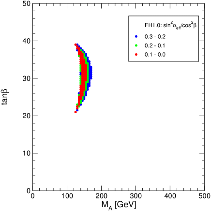
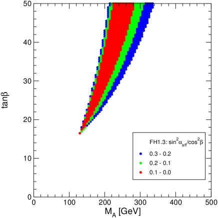
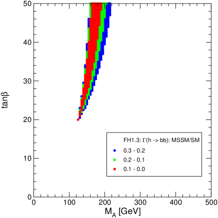
Figure 4: Regions of significant suppression of the coupling of $h$ to down-type fermions in the $M_{A}$–$\tan\beta$-plane within the “small $\alpha_{\rm eff}$” benchmark scenario. The upper left plot shows the ratio $\sin^{2}\alpha_{\rm eff}/\cos^{2}\beta\hskip 2.84526pt$ as evaluated with FeynHiggs1.0 (i.e. without ${\cal O}(\alpha_{b}\alpha_{s})$ and ${\cal O}(\alpha_{b}(\alpha_{s}\tan\beta)^{n})$ corrections), while the upper right plot shows the same quantity as evaluated with FeynHiggs1.3 (i.e. including these corrections). The plot in the lower row shows the ratio $\Gamma(h\rightarrow b\bar{b})_{\rm MSSM}\,/\,\Gamma(h\rightarrow b\bar{b})_{\rm SM}$, i.e. the partial width for $h\to b\bar{b}$ normalized to its SM value, where the other term in eq. (10) and further genuine loop corrections are taken into account (see text).

The effects of the higher-order corrections to the couplings of the lightest Higgs boson to the down-type fermions appear very pronounced in the “small $\alpha_{\rm eff}$” scenario [29], corresponding to the following choice of MSSM parameters:

$$m_{t}\,=\,174.3\,\,\mathrm{GeV},\quad M_{\rm SUSY}\,=\,800\,\,\mathrm{GeV},\quad X_{t}^{\rm FD}=\,-1100\,\,\mathrm{GeV}$$

$$\mu\,=\,2.5\,M_{\rm SUSY},\quad M_{2}\,=\,500\,\,\mathrm{GeV},\quad A_{b}\,=\,A_{t},\quad m_{\tilde{g}}\,=\,500\,\,\mathrm{GeV}~{}.$$ (11)

In the upper row of Fig. 4 we show the ratio $\sin^{2}\alpha_{\rm eff}/\cos^{2}\beta\hskip 2.84526pt$ in the $M_{A}$–$\tan\beta$ plane, evaluated in the “small $\alpha_{\rm eff}$” scenario. As explained above, replacing $\alpha$ by $\alpha_{\rm eff}$ in the tree-level couplings of eq. (9) gives rise to regions in the $M_{A}$–$\tan\beta$ plane where the effective coupling of the lightest Higgs boson to the down-type fermions is significantly suppressed with respect to the Standard Model. The region of significant suppression of $\sin^{2}\alpha_{\rm eff}/\cos^{2}\beta\hskip 2.84526pt$ as evaluated with FeynHiggs1.0, i.e. without the inclusion of the sbottom corrections beyond one-loop order, is shown in the upper left plot. The upper right plot shows the corresponding result as evaluated with FeynHiggs1.3, where the ${\cal O}(\alpha_{b}\alpha_{s})$ and ${\cal O}(\alpha_{b}(\alpha_{s}\tan\beta)^{n})$ corrections as well as the new ${\cal O}(\alpha_{t}^{2})$ ones are included. The new corrections are seen to have a drastic impact on the region where $\sin^{2}\alpha_{\rm eff}/\cos^{2}\beta\hskip 2.84526pt$ is small. While without the new corrections a suppression of 70% or more occurs only in a small area of the $M_{A}$–$\tan\beta$-plane for $20\;\raisebox{-3.00003pt}{$\stackrel{{\scriptstyle\displaystyle<}}{{\sim}}$}\;\tan\beta\;\raisebox{-3.00003pt}{$\stackrel{{\scriptstyle\displaystyle<}}{{\sim}}$}\;40$ and $100\,\,\mathrm{GeV}\;\raisebox{-3.00003pt}{$\stackrel{{\scriptstyle\displaystyle<}}{{\sim}}$}\;M_{A}\;\raisebox{-3.00003pt}{$\stackrel{{\scriptstyle\displaystyle<}}{{\sim}}$}\;200\,\,\mathrm{GeV}$, the region where $\sin^{2}\alpha_{\rm eff}/\cos^{2}\beta\hskip 2.84526pt$ is very small becomes much larger once these corrections are included. It now reaches from $\tan\beta\;\raisebox{-3.00003pt}{$\stackrel{{\scriptstyle\displaystyle>}}{{\sim}}$}\;15$ to $\tan\beta>50$, and from $M_{A}\;\raisebox{-3.00003pt}{$\stackrel{{\scriptstyle\displaystyle>}}{{\sim}}$}\;100\,\,\mathrm{GeV}$ to $M_{A}\;\raisebox{-3.00003pt}{$\stackrel{{\scriptstyle\displaystyle<}}{{\sim}}$}\;350\,\,\mathrm{GeV}$. The main reason for the change is that the one-loop ${\cal O}(\alpha_{b})$ corrections to the Higgs-boson mass matrix, which for large $\tan\beta$ would prevent $\alpha_{\rm eff}$ from going to zero, are heavily suppressed by the resummation of the ${\cal O}(\alpha_{b}(\alpha_{s}\tan\beta)^{n})$ corrections in the bottom Yukawa coupling. This kind of suppression depends strongly on the chosen MSSM parameters, and especially on the sign of $\mu$.

In order to interpret the physical impact of the effective coupling shown in the upper row of Fig. 4, the $\Delta_{d}$ terms in eq. (10) as well as further genuine loop corrections occuring in the $h\to b\bar{b}$ process have to be taken into account. The effect of these contributions can be seen from the plot in the lower row of Fig. 4, where the ratio $\Gamma(h\rightarrow b\bar{b})_{\rm MSSM}\,/\,\Gamma(h\rightarrow b\bar{b})_{\rm SM}$ is shown, which has been evaluated by including all terms of eq. (10) as well as all further corrections described in Ref. [34]. The region where the partial width $\Gamma(h\rightarrow b\bar{b})$ within the MSSM is suppressed compared to its SM value is seen to be somewhat reduced and shifted towards smaller values of $M_{A}$ as compared to the region where $\sin^{2}\alpha_{\rm eff}/\cos^{2}\beta\hskip 2.84526pt$ is small.

4 Estimate of the theoretical accuracy of the Higgs-boson mass determination

The prediction for $m_{h}$ in the MSSM is affected by two kinds of uncertainties, parametric uncertainties from the experimental errors of the input parameters and uncertainties from unknown higher-order corrections. While currently the parametric uncertainties dominate over those from unknown higher-order corrections, as the present experimental error of the top-quark mass of about $\pm 5$ GeV induces an uncertainty of $\Delta m_{h}\approx\pm 5$ GeV [33], at the next generation of colliders $m_{t}$ will be measured with a much higher precision, reaching the level of about 0.1 GeV at an $e^{+}e^{-}$ LC [36]. Thus, a precise measurement of $m_{h}$ will provide a high sensitivity to SUSY loop effects and will in this way allow a stringent test of the MSSM, provided that the uncertainties from unknown higher-order corrections are sufficiently well under control.

Given our present knowledge of the two-loop contributions to the Higgs-boson self-energies, the theoretical accuracy reached in the prediction for the ${\cal CP}$-even Higgs-boson masses is quite advanced. However, obtaining a complete two-loop result for the Higgs-boson masses and mixing angle requires additional contributions that are not yet available. In this section we discuss the possible effect of the missing two-loop corrections, and we estimate the size of the higher-order (i.e. three-loop) contributions.

4.1 Missing two-loop corrections

It is customary to separate the corrections to the Higgs boson self-energies into two parts: i) the momentum-independent part, namely the contributions to the self-energies evaluated at zero external momenta, which can also be computed in the effective potential approach; ii) the momentum-dependent corrections, i.e. the effects induced by the dependence on the external momenta of the self-energies, that are required to determine the poles of the $h,H$-propagator matrix.

All the presently known two-loop contributions are computed at zero external momentum, and moreover they are obtained in the so-called gaugeless limit, namely by switching off the electroweak gauge interactions. The two approximations are in fact related, since the leading Yukawa corrections are obtained by neglecting both the momentum dependence and the gauge interactions. In order to systematically improve the result beyond the approximation of the leading Yukawa terms, both effects from the gauge interactions and the momentum dependence should be taken into account.

In the limit where the momentum dependence and the gauge interactions are neglected, the only missing contributions are the mixed two-loop Yukawa terms, ${\cal O}(\alpha_{t}\alpha_{b})$, and the ${\cal O}(\alpha_{b}^{2})$ corrections (and analogous contributions proportional to the Yukawa couplings of the other fermions and sfermions, which however are expected to give significantly smaller contributions than the third generation quarks and scalar quarks). As in the case of the ${\cal O}(\alpha_{b}\alpha_{s})$ corrections, they can be numerically relevant only for large values of $\tan\beta$ and of the $\mu$ parameter. Concerning the ${\cal O}(\alpha_{t}\alpha_{b})$ corrections, although their computation is not yet available, it is plausible to assume that the most relevant contributions are connected to the threshold effects in the bottom mass coming from chargino–stop loops [16], which are actually already implemented in FeynHiggs as an additional option. An estimate of the ${\cal O}(\alpha_{b}^{2})$ corrections for a simplified choice of the MSSM parameters is presented in Ref. [14]. According to that discussion, their effect can be at most comparable to that of the genuine ${\cal O}(\alpha_{b}\alpha_{s})$ corrections, the latter being exemplified in Fig. 2 by the difference between the dashed and solid curves.

To try to estimate, although in a very rough way, the importance of the various contributions we look at their relative size in the one-loop part. There, in the effective potential part, the effect of the ${\cal O}(\alpha_{t})$ corrections typically amounts to an increase in $m_{h}$ of 40–60 GeV, depending on the choice of the MSSM parameters, whereas the corrections due to the electroweak (D-term) Higgs–squark interactions usually decrease $m_{h}$ by less than 5 GeV [4]. Instead, the purely electroweak gauge corrections to $m_{h}$, namely those coming from Higgs, gauge boson and chargino or neutralino loops [6], are typically quite small at one-loop, and can reach at most 5 GeV in specific regions of the parameter space (namely for large values of $\mu$ and $M_{2}$). Concerning the effects induced by the dependence on the external momentum, as a general rule we expect them to be more relevant in the determination of the heaviest eigenvalue $m_{H}$ of the Higgs-boson mass matrix, and when $M_{A}$ is larger than $M_{Z}$. Indeed, only in this case the self-energies are evaluated at external momenta comparable to or larger than the masses circulating into the dominant loops. In addition, if $M_{A}$ is much larger than $M_{Z}$, the relative importance of these corrections decreases, since the tree-level value of $m_{H}$ grows with $M_{A}$. In fact, the effect of the one-loop momentum-dependent corrections on $m_{h}$ amounts generally to less than 2 GeV.

Assuming that the relative size of the two-loop contributions follows a pattern similar to the one-loop part, we estimate that the two-loop diagrams involving D-term interactions should induce a variation in $m_{h}$ of at most 1–2 GeV, while we expect those with pure gauge electroweak interactions to contribute to $m_{h}$ not very significantly, probably of the order of 1 GeV or less. Given the smallness of the one-loop contribution it seems quite unlikely that the effect of the momentum-dependent part of the ${\cal O}(\alpha_{t}\alpha_{s})$ corrections to $m_{h}$, which should be the largest among this type of two-loop contributions, could be larger than 1 GeV. As already said, the situation can, in principle, be different for the heavier Higgs-boson mass. However, the corrections to $m_{H}$ are relatively small in general and at one-loop level for most parts of the MSSM parameter space the momentum-dependent corrections are not particularly relevant. The momentum-dependent corrections turn out to be more relevant in processes where the $H$ boson appears as an external particle, see Ref. [37].

Another way of estimating the uncertainties of the kind discussed above is to investigate the renormalization scale dependence introduced via the $\overline{\rm{DR}}$ definition of $\tan\beta$, $\mu$, and the Higgs field renormalization constants. Varying the scale parameter between $0.5m_{t}$ and $2m_{t}$ gives rise to a shift in $m_{h}$ of about $\pm 1.5$ GeV [23], in accordance with the estimates above.

4.2 Estimate of the uncertainties from unknown three-loop corrections

Even in the case that a complete two-loop computation of the MSSM Higgs masses is achieved, non-negligible uncertainties will remain, due to the effect of higher-order corrections. Although a three-loop computation of the Higgs masses is not available so far, it is possible to give at least a rough estimate for the size of these unknown contributions.

A first estimate can be obtained by varying the renormalization scheme in which the parameters entering the two-loop part of the corrections are expressed. In fact, the resulting difference in the numerical results amounts formally to a three-loop effect. Since the ${\cal O}(\alpha_{t}\alpha_{s}+\alpha_{t}^{2})$ corrections are particularly sensitive to the value of the top mass, we compare the predictions for $m_{h}$ obtained using in the two-loop corrections either the top pole mass, $m_{t}^{\rm pole}=174.3\,\,\mathrm{GeV}$, or the SM running top mass $\overline{m}_{t}$, expressed in the $\overline{\rm{MS}}$ renormalization scheme, i.e.

$$\overline{m}_{t}\;\;\equiv\;\;m_{t}(m_{t})^{\overline{\rm{MS}}}_{\mathrm{SM}}\;\;\simeq\;\;\frac{m_{t}^{\rm pole}}{1+4\,\alpha_{s}(m_{t})/3\pi-\alpha_{t}(m_{t})/2\pi}~{}.$$ (12)

Figure 5: $m_{h}$ as a function of $X_{t}$, using either $m_{t}^{\rm pole}$ or $\overline{m}_{t}$ in the two-loop corrections. The relevant MSSM parameters are chosen as $\tan\beta=3\,,\,M_{\rm SUSY}=M_{A}=\mu=1\,\,\mathrm{TeV}$ and $m_{\tilde{g}}=800\,\,\mathrm{GeV}$. For the different lines see text.

Inserting appropriate values for the SM running couplings $\alpha_{s}$ and $\alpha_{t}$ we find $\overline{m}_{t}=168.6\,\,\mathrm{GeV}$. In Fig. 5 we show the effect of changing the renormalization scheme for $m_{t}$ in the two-loop part of the corrections. The relevant MSSM parameters are chosen as in Fig. 1, i.e. $\tan\beta=3\,,\;M_{\rm SUSY}=M_{A}=\mu=1\,\,\mathrm{TeV}$ and $m_{\tilde{g}}=800\,\,\mathrm{GeV}$. The dot–dashed and dotted curves show the ${\cal O}(\alpha_{t}\alpha_{s})$ predictions for $m_{h}$ obtained using $m_{t}^{\rm pole}$ or $\overline{m}_{t}$, respectively, in the two-loop corrections. The solid and dashed curves, instead, show the corresponding ${\cal O}(\alpha_{t}\alpha_{s}+\alpha_{t}^{2})$ predictions for $m_{h}$. The difference in the two latter curves induced by the shift in $m_{t}$, which should give an indication of the size of the unknown three-loop corrections, is of the order of 1–1.5 GeV. However, as can be seen from the figure, the effect of the shift in $m_{t}$ partially cancels between the ${\cal O}(\alpha_{t}\alpha_{s})$ and ${\cal O}(\alpha_{t}^{2})$ corrections and there is no guarantee that such a compensating effect will appear again in the three-loop corrections.

An alternative way of estimating the typical size of the leading three-loop corrections makes use of the renormalization group approach. If all the supersymmetric particles (including the ${\cal CP}$-odd Higgs boson $A$) have mass $M_{\rm SUSY}$, and $\beta=\pi/2$, the effective theory at scales below $M_{\rm SUSY}$ is just the SM, with the role of the Higgs doublet played by the doublet that gives mass to the up-type quarks. In this simplified case, it is easy to apply the techniques of Refs. [19, 20] in order to obtain the leading logarithmic corrections to $m_{h}$ up to three loops (see also Ref. [38]). Considering for further simplification the case of zero stop mixing, we find:

$$\left(\Delta m_{h}^{2}\right)^{\rm LL}=\frac{3\,\alpha_{t}\,\overline{m}_{t}^{2}}{\pi}\,t\,\left[\,1+\left(\frac{3}{8}\,\alpha_{t}-2\,\alpha_{s}\right)\,\frac{t}{\pi}+\left(\frac{23}{6}\,\alpha_{s}^{2}-\frac{5}{4}\,\alpha_{s}\alpha_{t}-\frac{33}{64}\,\alpha_{t}^{2}\right)\,\frac{t^{2}}{\pi^{2}}\,+...\,\right]\;,$$ (13)

where $t=\log\,(M_{\rm SUSY}^{2}/\overline{m}_{t}^{2})$, $\overline{m}_{t}$ is defined in eq. (12), $\alpha_{t}$ and $\alpha_{s}$ have to be interpreted as SM running quantities computed at the scale $Q=\overline{m}_{t}$, and the ellipses stand for higher loop contributions. It can be checked that, for $M_{\rm SUSY}=1\,\,\mathrm{TeV}$, the effect of the three-loop leading logarithmic terms amounts to an increase in $m_{h}$ of the order of 1–1.5 GeV. If $M_{\rm SUSY}$ is pushed to larger values, the relative importance of the higher-order logarithmic corrections obviously increases. In that case, it becomes necessary to resum the logarithmic corrections to all orders, by solving the appropriate renormalization group equations numerically. Since it is unlikely that a complete three-loop diagrammatic computation of the MSSM Higgs-boson masses will be available in the near future, it will probably be necessary to combine different approaches (e.g. diagrammatic, effective potential and renormalization group), in order to improve the accuracy of the theoretical predictions up to the level required to compare with the experimental results expected at the next generation of colliders.

To summarize this discussion, the uncertainty in the prediction for the lightest ${\cal CP}$-even Higgs boson arising from not yet calculatated three-loop and even higher-order corrections can conservatively be estimated to be 1–2 GeV. From the various missing two-loop corrections an uncertainty of less than 3 GeV is expected. However, it is extremely unlikely that all these effects would coherently sum up, with no partial compensation among them. Therefore we believe that a realistic estimate of the uncertainty from unknown higher-order corrections in the theoretical prediction for the lightest Higgs boson mass should not exceed $3\,\,\mathrm{GeV}$.

5 Conclusions

In this paper we have discussed the phenomenological impact of recently obtained results in the MSSM Higgs sector. The new corrections have now been implemented in the code FeynHiggs, which in this way provides the currently most precise evaluation of the masses and mixing angles of the ${\cal CP}$-even MSSM Higgs sector. We have analyzed the effects of these new contributions by comparing the results obtained with FeynHiggs1.3, the newest version of the code that incorporates all these effects, with those derived with previous versions in which the two-loop ${\cal O}(\alpha_{t}^{2})$ corrections were implemented via a renormalization group method and the sbottom corrections beyond one-loop were not taken into account.

As a result of these improvements the lower limits on $\tan\beta\hskip 2.84526pt$ that can be derived by combining the theoretical upper bound on $m_{h}$ with its experimental lower bound, are significantly weakened. We have also shown that, if the top-quark mass is increased by one standard deviation, the constraint on $\tan\beta\hskip 2.84526pt$ completely disappears if the other MSSM parameters are such that $m_{h}$ takes its maximum value as a function of $\tan\beta$.

Concerning the coupling of the lightest Higgs boson to the down-type fermions, that is related to the angle that diagonalizes the Higgs boson mass matrix including higher order corrections, we have shown that the area in the $M_{A}$–$\tan\beta$-plane where its value gets suppressed by $70\%$ or more with respect to the SM one is significantly modified.

Finally, we have given an estimate of the uncertainties related to the various kinds of two- and three-loop contributions to the Higgs boson masses that are still unknown. Since it is extremely unlikely that all these effects would coherently sum up, the uncertainty in the theoretical prediction for the lightest MSSM Higgs boson mass from unknown two- and three-loop corrections should not exceed $3\,\,\mathrm{GeV}$.

References

-
[1]
H.P. Nilles,
Phys. Rep. 110 (1984) 1;
H.E. Haber and G.L. Kane, Phys. Rep. 117, (1985) 75;
R. Barbieri, Riv. Nuovo Cim. 11, (1988) 1. - [2] J. Gunion, H. Haber, G. Kane and S. Dawson, The Higgs Hunter’s Guide, Addison-Wesley, 1990.
-
[3]
J. Ellis, G. Ridolfi and F. Zwirner,
Phys. Lett. B 257, 83 (1991);
Y. Okada, M. Yamaguchi and T. Yanagida, Prog. Theor. Phys. 85, 1 (1991);
H. Haber and R. Hempfling, Phys. Rev. Lett. 66, 1815 (1991). - [4] A. Brignole, Phys. Lett. B 281 (1992) 284.
- [5] P. Chankowski, S. Pokorski and J. Rosiek, Phys. Lett. B 286 (1992) 307; Nucl. Phys. B 423 (1994) 423, hep-ph/9303309.
- [6] A. Dabelstein, Nucl. Phys. B 456 (1995) 25, hep-ph/9503443; Z. Phys. C 67 (1995) 495, hep-ph/9409375.
- [7] R. Hempfling and A. Hoang, Phys. Lett. B 331 (1994) 99, hep-ph/9401219.
- [8] S. Heinemeyer, W. Hollik and G. Weiglein, Phys. Rev. D 58 (1998) 091701, hep-ph/9803277; Phys. Lett. B 440 (1998) 296, hep-ph/9807423.
- [9] S. Heinemeyer, W. Hollik and G. Weiglein, Eur. Phys. Jour. C 9 (1999) 343, hep-ph/9812472.
-
[10]
R. Zhang, Phys. Lett. B 447 (1999) 89,
hep-ph/9808299;
J. Espinosa and R. Zhang, JHEP 0003 (2000) 026, hep-ph/9912236. - [11] G. Degrassi, P. Slavich and F. Zwirner, Nucl. Phys. B 611 (2001) 403, hep-ph/0105096.
- [12] J. Espinosa and R. Zhang, Nucl. Phys. B 586 (2000) 3, hep-ph/0003246.
- [13] A. Brignole, G. Degrassi, P. Slavich and F. Zwirner, Nucl. Phys. B 631 (2002) 195, hep-ph/0112177.
- [14] A. Brignole, G. Degrassi, P. Slavich and F. Zwirner, Nucl. Phys. B 643 (2002) 79, hep-ph/0206101.
-
[15]
T. Banks,
Nucl. Phys. B 303 (1988) 172;
L. Hall, R. Rattazzi and U. Sarid, Phys. Rev. D 50 (1994) 7048, hep-ph/9306309;
R. Hempfling, Phys. Rev. D 49 (1994) 6168;
M. Carena, M. Olechowski, S. Pokorski and C. Wagner, Nucl. Phys. B 426 (1994) 269, hep-ph/9402253. - [16] M. Carena, D. Garcia, U. Nierste and C. Wagner, Nucl. Phys. B 577 (2000) 577, hep-ph/9912516.
-
[17]
S. Heinemeyer, W. Hollik and G. Weiglein, Comp. Phys. Comm. 124 2000 76,
hep-ph/9812320;
hep-ph/0002213.
The codes are accessible via www.feynhiggs.de . - [18] M. Frank, S. Heinemeyer, W. Hollik and G. Weiglein, hep-ph/0202166.
-
[19]
M. Carena, J. Espinosa, M. Quirós and C. Wagner,
Phys. Lett. B 355 (1995) 209,
hep-ph/9504316;
M. Carena, M. Quirós and C. Wagner, Nucl. Phys. B 461 (1996) 407, hep-ph/9508343. - [20] H. Haber, R. Hempfling and A. Hoang, Z. Phys. C 75 (1997) 539, hep-ph/9609331.
- [21] S. Heinemeyer, W. Hollik, J. Rosiek and G. Weiglein, Eur. Phys. Jour. C 19 (2001) 535, hep-ph/0102081.
-
[22]
W. Siegel,
Phys. Lett. B 84 (1979) 193;
D. Capper, D. Jones, P. van Nieuwenhuizen, Nucl. Phys. B 167 (1980) 479. - [23] M. Frank, S. Heinemeyer, W. Hollik and G. Weiglein, in preparation.
- [24] A. Freitas and D. Stöckinger, hep-ph/0210372.
- [25] S. Heinemeyer, W. Hollik and G. Weiglein, hep-ph/9910283.
- [26] M. Carena, H. Haber, S. Heinemeyer, W. Hollik, C. Wagner and G. Weiglein, Nucl. Phys. B 580 (2000) 29, hep-ph/0001002.
- [27] J. Espinosa and I. Navarro, Nucl. Phys. B 615 (2001) 82, hep-ph/0104047.
- [28] [LEP Higgs working group], hep-ex/0107030.
- [29] M. Carena, S. Heinemeyer, C. Wagner and G. Weiglein, hep-ph/9912223; to appear in Eur. Phys. Jour. C, hep-ph/0202167.
- [30] B. Allanach et al., Eur. Phys. Jour. C 25 (2002) 113, hep-ph/0202233.
- [31] A. Quadt, private communication.
-
[32]
[LEP Higgs working group], LHWG Note/2002-01,
http://lephiggs.web.cern.ch/LEPHIGGS/papers/. - [33] S. Heinemeyer, W. Hollik and G. Weiglein, JHEP 0006 (2000) 009, hep-ph/9909540.
- [34] S. Heinemeyer, W. Hollik and G. Weiglein, Eur. Phys. Jour. C 16 (2000) 139, hep-ph/0003022.
-
[35]
M. Carena, S. Mrenna and C. Wagner,
Phys. Rev. D 60 (1999) 075010,
hep-ph/9808312;
Phys. Rev. D 62 (2000) 055008,
hep-ph/9907422;
H. Eberl, K. Hidaka, S. Kraml, W. Majerotto and Y. Yamada, Phys. Rev. D 62 (2000) 055006, hep-ph/9912463. - [36] TESLA TDR Part 3: Physics at an Linear Collider, eds. R.D. Heuer, D. Miller, F. Richard and P.M. Zerwas, hep-ph/0106315,
- [37] T. Hahn, S. Heinemeyer and G. Weiglein, hep-ph/0211204.
- [38] A. Hoang, Applications of Two-Loop Calculations in the Standard Model and its Minimal Supersymmetric Extension, PhD thesis, Universität Karlsruhe, Shaker Verlag, Aachen 1995.
- [39] S. Martin, hep-ph/0211366.
- [40] S. Martin, Phys. Rev. D 65 (2002) 116003, hep-ph/0111209; Phys. Rev. D 66 (2002) 096001, hep-ph/0206136.