Baryon inhomogeneity generation via cosmic strings at QCD scale and its effects on nucleosynthesis

Abstract

We have earlier shown that cosmic strings moving through the plasma at the time of a first order quark-hadron transition in the early universe can generate large scale baryon inhomogeneities. In this paper, we calculate detailed structure of these inhomogeneities at the quark-hadron transition. Our calculations show that the inhomogeneities generated by cosmic string wakes can strongly affect nucleosynthesis calculations. A comparison with observational data suggests that such baryon inhomogeneities should not have existed at the nucleosynthesis epoch. If this disagreement holds with more accurate observations, then it will lead to the conclusions that cosmic string formation scales above $10^{14}-10^{15}$ GeV may not be consistent with nucleosynthesis and CMBR observations. Alternatively, some other input in our calculation should be constrained, for example, if the average string velocity remains sufficiently small so that significant density perturbations are never produced at the QCD scale, or if strings move ultra-relativistically so that string wakes are very thin, trapping negligible amount of baryons. Finally, if quark-hadron transition is not of first order then our calculations do not apply.

I Introduction

Recent measurements of the cosmic microwave background radiation (CMBR) anisotropy have reached a sufficiently high level of precision that stringent bounds can be put on various cosmological parameters such as baryon to entropy ratio $\eta$. It is certainly quite remarkable that the calculations of standard big-bang nucleosynthesis (SBBN) are reasonably consistent with these stringent bounds on $\eta$. Though several modifications to SBBN are still being considered to better account for the abundances of light elements. One such possibility discussed extensively in the literature is the so called inhomogeneous big bang nucleosynthesis (IBBN) [1, 2] where nucleosynthesis takes place in the presence of baryon number inhomogeneities. Various models have been worked out where inhomogeneities of a particular shape and size are taken and their effects on nucleosynthesis are calculated. Different values of the light elemental abundances are calculated and compared with the observed values [2]. These calculations are supplemented with the investigations of baryon inhomogeneity generation during a first order quark-hadron phase transition [3, 4]. Though, it is fair to say that current observations do not support any strong deviation from the SBBN calculations. Calculations of IBBN, such as those in ref. [1, 2], therefore, can be used to constrain the presence of baryon fluctuations in the early universe.

In a previous paper [5], we had shown that baryon inhomogeneities on large-scales will be generated by cosmic string wakes during the quark-hadron transition. This arises due to the fact that when there are density fluctuations present in the universe, (for example, those which eventually lead to the formation of structure we see today), then resulting temperature fluctuations, even if they are of small magnitude, can affect the dynamics of a first order phase transition in crucial ways. There have been many discussions of the effects of inhomogeneities on the dynamics of a first order quark-hadron transition in the universe [6, 7]. For example, Christiansen and Madsen have discussed [6] heterogeneous nucleation of hadronic bubbles due to presence of impurities. Hadronic bubbles are expected to nucleate at these impurities with enhanced rates. Recently, Ignatius and Schwarz have proposed [7] that the presence of density fluctuations (those arising from inflation) at quark-hadron transition will lead to splitting of the region in hot and cold regions with cold regions converting to hadronic phase first. Baryons will then get trapped in the (initially) hotter regions. Estimates of sizes and separations of such density fluctuations were made in ref.[7] using COBE measurements of the temperature fluctuations in CMBR. In ref. [5], we considered the effect of cosmic string induced density fluctuations on quark-hadron transition and showed that it can lead to formation of extended planar regions of baryon inhomogeneity.

We mention here again, as discussed in ref.[5], that there has been extensive study of density fluctuations generated by cosmic strings from the point of view of structure formation [8], and it is reasonably clear that recent measurements of temperature anisotropies in the microwave background by BOOMERANG, and MAXIMA experiments [9] at angular scales of $\ell\simeq$ 200 disfavor models of structure formation based exclusively on cosmic strings [10, 11]. However, even with present models of cosmic string network evolution, it is not ruled out that cosmic strings may contribute to some part in the structure formation in the universe. Further, cosmic strings generically arise in many Grand Unified Theory (GUT) models. If the GUT scale is somewhat lower than $10^{16}$ GeV then the resulting cosmic strings will not be relevant for structure formation (for a discussion of these issues, see [11]). However, they may still affect various stages of the evolution of the universe in important ways. Our study in ref.[5] (see, also ref.[12]), and the present study are motivated from this point of view.

In this paper we determine the detailed structure of the baryon inhomogeneities created by the cosmic string wakes [5]. We find that the magnitude and length scale of these inhomogeneities are such that they should survive until the stage of nucleosynthesis, affecting the calculations of abundances of light elements. A comparison with observational data suggests that such baryon inhomogeneities should not have existed at the nucleosynthesis epoch. If this disagreement holds with more accurate observations then it will lead to the conclusion that cosmic string formation scales above $10^{14}-10^{15}$ GeV may not be consistent with nucleosynthesis and CMBR observations. Alternatively, some other input in our calculation should be constrained, for example, if the average string velocity remains sufficiently small so that significant density perturbations are never produced at the QCD scale, or if strings move ultra-relativistically so that string wakes are very thin, trapping negligible amount of baryons. Of course entire discussion of this paper is applicable only when quark-hadron transition is of first order.

The paper is organized in the following manner. In section II, we briefly discuss the nature of density fluctuations as expected from cosmic strings moving through a relativistic fluid. In section III we discuss the dynamics of quark-hadron transition in the presence of string wakes, and discuss how baryons are concentrated in sheet like regions inside these wakes. Section IV discusses the results of our calculations where we present the detailed structure of the baryon inhomogeneities. In section V we discuss the effects, these baryon inhomogeneities surviving until the nucleosynthesis stage, can have on the abundances of light elements, and discuss the constraints on the cosmic string models arising from observations of various abundances. Conclusions are presented in section VI.

II Density Fluctuations arising due to Straight Cosmic Strings

In this section we briefly review the structure of density fluctuations produced by a cosmic string moving through a relativistic fluid. The space-time around a straight cosmic string (along the z axis) is given by the following metric [13],

$$ds^{2}=dt^{2}-dz^{2}-dr^{2}-(1-4G\mu)^{2}r^{2}d\psi^{2},$$ (1)

where $\mu$ is the string tension. This metric describes a conical space, with a deficit angle of $8\pi G\mu$. This metric can be put in the form of the Minkowski metric by defining angle $\psi^{\prime}=(1-4G\mu)\psi$. However, now $\psi^{\prime}$ varies between 0 and $(1-4G\mu)2\pi$, that is, a wedge of opening angle $8\pi G\mu$ is removed from the Minkowski space, with the two boundaries of the wedge being identified. It is well known that in this space-time, two geodesics going along the opposite sides of the string, bend towards each other [14]. This results in binary images of distant objects, and can lead to planar density fluctuations. These wakes arise as the string moves through the background medium, giving rise to velocity impulse for the particles in the direction of the surface swept by the moving string. For collisionless particles the resulting velocity impulse is [8, 15], $v_{impls}\simeq 4\pi G\mu v_{st}\gamma_{st}$ (where $v_{st}$ is the transverse velocity of the string). This leads to a wedge like region of overdensity, with the wedge angle being of order of the deficit angle, i.e. $8\pi G\mu$ ($\sim 10^{-5}$ for 10¹⁶ GeV GUT strings). The density fluctuation in the wake is of order one.

The structure of this wake is easy to see for collisionless particles (whether non-relativistic, or relativistic). Each particle trajectory passing by the string bends by an angle of order $4\pi G\mu$ towards the string. In the string rest frame, take the string to be at the origin, aligned along the z axis, such that the particles are moving along the $-x$ axis. Then it is easy to see that particles coming from positive $x$ axis in the upper/lower half plane will all be above/below the line making an angle $\mp 4\pi G\mu$ from the negative $x$ axis. This implies that the particles will overlap in the wedge of angle $8\pi G\mu$ behind the string leading to a wake with density twice of the background density. One thus expects a wake with half angle $\theta_{w}$ and an overdensity $\delta\rho/\rho$ where [8, 15],

$$\theta_{w}\sim 4\pi G\mu,\qquad{\delta\rho\over\rho}\sim 1.$$ (2)

However, the case of relevance for us is cosmic strings moving through a relativistic plasma of elementary particles at temperatures of order 100 MeV. At that stage, it is not proper to take the matter as consisting of collisionless particles. A suitable description of matter at that stage is in terms of a relativistic fluid which we will take to be an ideal fluid consisting of elementary particles. Generation of density fluctuations due to a cosmic string moving through a relativistic fluid has been analyzed in the literature [16, 17, 18]. The study in ref.[16] focused on the properties of shock formed due to supersonic motion of the string through the fluid. In the weak shock approximation, one finds a wake of overdensity behind the string. In this treatment one can not get very strong shocks with large overdensities. In refs. [17, 18], a general relativistic treatment of the shock was given which is also applicable for ultra-relativistic string velocities. The treatment in ref.[18] is more complete in the sense that the equations of motion of a relativistic fluid are solved in the string space-time (Eq.(1)), and both subsonic and supersonic flows are analyzed. One finds that for supersonic flow, a shock develops behind the string, just as in the study of ref. [16, 17]. In the treatment of ref.[18] one recovers the usual wake structure of overdensity (with the wake angle being of order $G\mu$) as the string approaches ultra-relativistic velocities. Also the overdensity becomes of order one in this regime.

However, it is not expected that the string will move with ultra-relativistic velocities in the early universe. Various simulations have shown [19] that rms velocity of string segments is about 0.6 for which the shock will be weak. For this case, the half angle of the wedge $\theta_{w}$ will also be large. We use expressions from ref.[18] which are also valid for the ultra-relativistic case. Resulting density fluctuation in the wake of the moving string is expressed in terms of fluid and sound four velocities,

$${\delta\rho\over\rho}\simeq{16\pi G\mu u_{f}^{2}(1+u_{s}^{2})\over 3u_{s}\sqrt{u_{f}^{2}-u_{s}^{2}}},\qquad sin\theta_{w}\simeq{u_{s}\over u_{f}},$$ (3)

where $u_{f}=v_{f}/\sqrt{1-v_{f}^{2}}$ and $u_{s}=v_{s}/\sqrt{1-v_{s}^{2}}$, with $v_{s}$ being the sound speed. In this case, when string velocity $v_{f}$ is ultra-relativistic, then one can get strong overdensities (of order 1) and the angle of the wake approaches the deficit angle $\simeq 8\pi G\mu$. As mentioned in ref.[5], in view of simulation results, we will use a sample value corresponding to string velocity of 0.9 for which we take,

$$\theta_{w}\simeq 20^{0},\qquad\delta\rho/\rho\simeq 3\times 10^{-5}.$$ (4)

These values correspond to those obtained from Eq.3 for $v_{s}=1/\sqrt{3}$. In the next section, we will study the effects of such wakes on the dynamics of a first order quark-hadron transition.

III Effect of string wakes on quark-hadron transition

In the conventional picture of the quark-hadron transition, the transition proceeds as follows [20]. As the universe cools below the critical temperature $T_{c}$ of the transition, hadronic bubbles of size larger than a certain critical size can nucleate in the QGP background. These bubbles will then grow, coalesce, and eventually convert the QGP phase to the hadronic phase [20, 21, 22, 23, 24, 6, 7]. Very close to $T_{c}$ the critical size of the bubbles is too large, and their nucleation rate too small, to be relevant for the transition. Universe must supercool down to a temperature $T_{sc}$ when the nucleation rate becomes significant. The actual duration of supercooling depends on various parameters such as the values of surface tension $\sigma$ and the latent heat $L$. We take the values of these parameters as in ref.[7] (motivated by lattice simulations [25]), $\sigma\simeq 0.015T_{c}^{3}$ and $L\simeq 3T_{c}^{4}$. With these values, one can estimate the amount of supercooling to be [7, 23] (we take $T_{c}=150$ MeV),

$$\Delta T_{sc}\equiv 1-{T_{sc}\over T_{c}}\simeq 10^{-4}.$$ (5)

(We mention here that it has been argued in the literature that the amount of supercooling may be smaller by many orders of magnitude [26]. In that situation, the density fluctuations of magnitude given in Eq.(4) will have even more prominent effect on the dynamics of quark-hadron transition.)

As the universe cools below $T_{sc}$, bubbles keep getting nucleated and keep expanding. This nucleation process is very rapid and lasts only for a temperature range of $\Delta T_{n}\simeq 10^{-6}$, for a time duration of order $\Delta t_{n}\simeq 10^{-5}t_{H}$ ($t_{H}$ is the Hubble time) [24, 7]. The latent heat released in the process of bubble expansion re-heats the universe. Eventually, the universe is reheated enough so that no further nucleation can take place. Further conversion of the QGP phase to the hadronic phase happens only by the expansion of bubbles which have been already nucleated. Even this expansion is controlled by how the latent heat is dissipated away from the bubble walls. Essentially, the universe cools little bit, allowing bubbles to expand and release more latent heat. After the phase of rapid bubble nucleation, the universe enters into the slow combustion phase [20]. As was discussed in ref.[5], the picture of this slow combustion phase is very different when cosmic string wakes are present. In the following we briefly review this discussion from ref.[5].

We take the parameters of the density fluctuations as given in Eq.(4). Density fluctuation $\delta\rho/\rho\simeq 3\times 10^{-5}$ translates to a temperature fluctuation of order $\Delta T_{wake}\equiv\delta T/T\simeq 10^{-5}$. We note that this temperature fluctuation is larger than $\Delta T_{n}\simeq 10^{-6}$. This means that the nucleation of hadronic bubbles will get completed in the QGP region outside the wake of the string, while nucleation in the wake region during that stage will be suppressed. Since $\Delta T_{sc}$ is not too different from $\Delta T_{wake}$, one can conclude that the outside region will enter a slow combustion phase before any significant bubble nucleation can take place in the region of overdensity in the wake. For this it is required that the overdensity in the wake should not decrease in the time scale of $\Delta t_{n}\simeq 10^{-5}t_{H}$. The typical average thickness of the overdense region in the shock $d_{shk}$ will be (for a wake extending across the horizon),

$$d_{shk}\simeq sin\theta_{w}~{}r_{H}\simeq 3km.$$ (6)

Where, $r_{H}=2t_{H}\simeq 10$ km is the horizon size. $t_{H}\simeq 30\mu sec$ is the age of the universe (at $T=T_{c}=150$ MeV). Typical time scale, $t_{shk}$, for the evolution of the overdensity in this region (which is smaller than the horizon size [27]), will be governed by the sound velocity $v_{s}$ which becomes very small close to the transition temperature (e.g.,$v_{s}\simeq 0.1$) [7, 21]. We get,

$$t_{shk}\simeq{d_{shk}\over v_{s}}>t_{H}.$$ (7)

Thus the density (and hence temperature) evolution in the shock region happens in a time scale which is too large compared to $\Delta t_{n}$. It is also much larger than $\Delta t_{trnsn}(\simeq 14\mu sec)$ during which the quark phase is completely converted to the hadronic phase in the region outside the wake. We mention that in our picture, we consider the time when the universe has just started going through the quark-hadron transition, and we focus on a region in which a wake of density fluctuation of size of order $r_{H}$ has been created by the moving string. Essentially the region of study for us is the horizon volume from which the string is just exiting at the time when the universe temperature $T=T_{sc}$. The formation of most of the region of shock thus happens when the temperature is still large enough compared to $T_{c}$ so that the speed of sound is close to the value 1/$\sqrt{3}$. However, some portion of the wake will certainly form when the temperature is close enough to $T_{c}$, that the relevant sound speed is small, say, $v_{s}\simeq 0.1$. The extent of the overdense region will be governed by the time scale $t_{shk}$. Thus, if $t_{shk}$ is much smaller than $t_{H}$, then wake will not extend across the horizon.

The precise time duration, $\Delta t_{lag}$, by which the process of bubble nucleation in the shock region lags behind that in the region outside the wake is given by [7, 24],

$$\Delta t_{lag}\simeq{\Delta T_{wake}t_{H}\over 3v_{s}^{2}}\simeq 10^{-5}t_{H},$$ (8)

with $v_{s}=1/\sqrt{3}$. $\Delta t_{lag}$ will be much larger if we take $v_{s}=0.1$. $\Delta t_{lag}$ is the extra time in which the temperature in the wake decreases to $T_{sc}$ compared to the time when the temperature drops to $T=T_{sc}$ in the region outside the wake. Since $\Delta t_{lag}$ is at least of same order as $\Delta t_{n}$, we conclude that the region outside the wake enters the slow combustion phase before any significant bubble nucleation can take place in the wake region. It is then reasonable to conclude that the latent heat released in the region outside the wake will suppress any bubble nucleation in the wake especially near the boundaries of the wake. If the heat propagates to the interior of the wake, then the bubble suppression may extend to the interior of the wake also, implying that there will simply be no bubbles in the entire wake region. In that case, hadronic bubbles which have been nucleated outside the wake will all coalesce and convert the entire outside region to the hadronic phase (with occasional QGP localized regions embedded in it). This hadronic region will be separated from the QGP region inside the wake by the interfaces at the boundaries of the wake, as shown in Fig.1.

Further completion of the phase transition will happen when these interfaces move inward from the wake boundaries. These moving, macroscopic, interfaces may trap most of the baryon number in the entire region of the wake (and some neighborhood) towards the inner region of the wake. Finally the interfaces will merge, completing the phase transition, and leading to a sheet of very large baryon number density, extending across the horizon. Actual value of baryon density in these sheets will depend on what fraction of baryon number is trapped in the QGP phase by moving interfaces, and we will determine that in the following.

It is also possible that the bubble nucleation is not entirely suppressed near the center of the shock region as the latent heat released by moving interfaces will have dominant effect locally. While the region outside the wake converts to the hadronic phase, same may happen at the center of the wake as well. In that case the hadronic phase will spread from inside the wake at the same time when the hadronic phase is moving in from outside the wake through the wake boundary. These two sets of interfaces will then lead to concentration of baryon number in two different sheet like regions, with the separation between the two sheets being of the order of a km or so. However, even in such a situation, the magnitude of the amplitude and the length scale of baryon inhomogeneity, as we determine below, will change only by a factor of about 2. Therefore, for simplicity of presentation, we will not consider this situation, and will only consider the case when only one sheet of baryon inhomogeneity is formed within the string wake. We also mention here that we are not considering the effect of density fluctuations produced by string loops. These will also lead to baryon number inhomogeneities via the effects discussed here. However, these structures will be on a more localized scale. It is more complicated to calculate the effects of density fluctuations by oscillating loops (especially when time scales are of crucial importance). Still, a more complete investigation of the effects of cosmic strings on quark-hadron transition should include this contribution also.

We now determine the detailed profile of the baryon inhomogeneity resulting from the above picture. For this, we have to calculate the evolution of baryon densities in the QGP phase and in the hadron phase as the transition proceeds. First, we note that typical separation between string wakes (and hence resulting baryonic sheets) will be governed by the number of long strings in a given horizon, which is expected to be about 15 (from numerical simulations [28]). The exact structure of these wakes in a given horizon volume needs to be known in order to study the concentration of baryons by advancing interfaces as the transition to hadronic phase proceeds. For example, if the string wakes are reasonably parallel, then they will span most of the horizon volume, as the average thickness of a wake (with parameters in Eq.(4)) will be order 1-2 km (a single string wake will not be expected to extend over the entire horizon). In such a situation, the hadronic phase will first appear in the regions between the wakes, which may cover a very small fraction of the horizon volume initially. The initial value of the fraction $f$ of the QGP phase to the hadronic phase will then be close to 1. $f$ will then slowly decrease to zero as the planar interfaces (formed by the coalescence of bubbles in the region in between the overdense wakes) move inward, converting the QGP region inside the wake into the hadronic phase. Certainly, the actual situation will be more complicated than this, with string wakes extending in random directions, and often even overlapping. In such a situation, even the initial value of $f$, when bubble coalescence (in the regions between the wakes) forming planar interfaces, may be smaller than 1 (though not much smaller). However, again, this does not affect the order of magnitude estimate of the profile of the resulting baryon inhomogeneity as we determine below. Therefore, we use a simple picture, by focusing on the region relevant for only one string, covering about 1/15 of the horizon volume. Further, we take the initial value of $f$ to be almost 1.

The baryon evolution in this overdense wake region and outside of this region will depend on the detailed dynamics of the phase boundary and the expansion of the universe during this epoch. To study this we will follow the calculations of Fuller et.al.[22] who have studied the evolution of the baryon fluctuations which might have been produced at the end of nucleation epoch during the QCD phase transition. In ref.[22], the evolution of baryon density in the QGP phase and in the hadron phase has been calculated as the hadronic region expands at the cost of the volume of the QGP phase during the co-existence temperature epoch. The main difference between their model and our model is that the QGP regions of interest for them are expected to be spherical, while in our case it is a thick sheet-like region, with planar interfaces separating the QGP region from the hadronic region.

Let us first recall the effect of the expansion of the Universe on the dynamics of the phase transition [22, 5]. If $R(t)$ is the scale factor of Robertson-Walker metric, then Einstein’s equations give [22, 5],

$${{\dot{R}(t)}\over R(t)}=\sqrt{{8\pi G\rho(t)\over 3}},$$ (9)

where $\rho$ is the average energy density of the mixed phase. The energy density, entropy density, and pressure ($\rho_{q},s_{q},p_{q}$) in the QGP phase and ($\rho_{h},s_{h},p_{h}$) in the hadronic phase are,

$$\rho_{q}=g_{q}aT^{4}+B,~{}s_{q}={4\over 3}g_{q}aT^{3},~{}p_{q}={g_{q}\over 3}aT^{4}-B$$ (10)

$$\rho_{h}=g_{h}aT^{4},~{}s_{h}={4\over 3}g_{h}aT^{3},~{}p_{h}={g_{h}\over 3}aT^{4}.$$ (11)

Here $g_{q}\simeq 51$ and $g_{h}\simeq 17$ are the degrees of freedom relevant for the two phases respectively (taking two massless quark flavors in the QGP phase, and counting other light particles) [22] and $a={\pi^{2}\over 30}$. At the transition temperature we have $p_{q}=p_{h}$ which relates $T_{c}$ and the bag constant $B$ as, $B={1\over 3}aT_{c}^{4}(g_{q}-g_{h})$. We define $x=g_{q}/g_{h}$ to be the ratio of degrees of freedom between the two phases. For the mixed phase, we write the average value of energy density as, $\rho=f\rho_{q}+(1-f)\rho_{h}$. Here $f$ denotes the fraction of the volume in the QGP phase. With this, Eq.(9) can be written as,

$${\dot{R}(t)\over R(t)}=({8\pi GB\over 3})^{1/2}[4f+{3\over{x-1}}]^{{1\over 2}}.$$ (12)

Now, conservation of the energy-momentum tensor gives,

$$R(t)^{3}{dp(t)\over dt}={d\over dt}\{R(t)^{3}[\rho(t)+p(t)]\}.$$ (13)

During the transition, $T$ and $p$ are approximately constant. With this, Eq.(13) can be rewritten as

$${{\dot{R}(t)}\over R(t)}=-{\dot{f}(x-1)\over 3f(x-1)+3}.$$ (14)

Eq.(12) and Eq.(14) along with the transport rate equations, which will be discussed bellow, will give the evolution of baryon densities in the quark gluon plasma phase and in the hadron phase. The evolution of baryon density can be studied in each phase as the interfaces move forward and baryons are transported from one phase to another. If $n_{b}^{q}$ and $n_{b}^{h}$ are the net baryon densities in the QGP phase and the hadron phase respectively, then their evolution equations are as follows [22]

$$\dot{n}_{b}^{q}=-n_{b}^{q}\lambda_{q}+n_{b}^{h}\lambda_{h}-n_{b}^{q}[{\dot{V}(t)\over V(t)}+{\dot{f}\over f}],$$ (15)

$$\dot{n}_{b}^{h}=[{f\over{1-f}}][-n_{b}^{h}\lambda_{h}+n_{b}^{q}\lambda_{q}+n_{b}^{h}{\dot{f}\over f}]-n_{b}^{h}{\dot{V}(t)\over V(t)},$$ (16)

where dot denotes the rate of change of the baryon density with time and $\lambda_{q}$, $\lambda_{h}$ are characteristic baryon transfer rates [22] from the QGP to hadron phase and hadron to QGP phase respectively. The definitions of these two quantities are discussed below. $V(t)$ is the volume of the region under consideration. The term ${\dot{V}(t)\over V(t)}$ arises due to expansion of the universe and is given by

$${\dot{V}(t)\over V(t)}=3{\dot{R}(t)\over R(t)}.$$ (17)

Now in our model, each cosmic string forms wake like overdensity leading the trapping of the QGP region in between two planar interfaces. Collapse of these two interfaces towards each other leads to the concentration of baryons which is the subject of study here. Numerical simulations have shown that in the scaling regime, there are $(10-15)$ strings [28] per horizon. For any reasonable GUT scale, strings are definitely in the scaling regime by the stage of the quark hadron phase transition epoch. Initial time relevant for us is the stage when planar interfaces have formed (by coalescence of hadronic bubbles in the regions in between the wakes of different strings) at the two boundaries of overdense wakes. At this stage, we take the initial volume relevant for each string as,

$$V_{0}\approx({1\over 15})r_{H}^{3},$$ (18)

where $r_{H}(=2t)$ is the size of the horizon at this initial time $t_{0}$. Note that we take the wake like overdense regions to be well formed at the time $t_{0}$. We take the simple picture that baryon concentration in each such volume is determined by the collapse of two interfaces at the boundary of wake of a single string, without getting significantly affected by the presence of wakes in the region outside the relevant comoving region. As mentioned earlier, this approximation should be o.k. for determining the order of magnitude of baryon overdensities etc. Thus our representative volume is, $V(t)=V_{0}({R(t)\over R_{0}})^{3}$.

Now let us define the terms $n_{b}^{q}\lambda_{q}$ and $n_{b}^{h}\lambda_{h}$ which appear in the transport rate equations Eq.(15) and Eq.(16). In our model the interface of the QGP region inside the string wake consists of two planar sheets. (This is in contrast to the situation in ref. [22] where the interface was a spherical surface). The area of each interface sheet is $A\sim V(t)^{2/3}$, assuming the planar interface extending over the region with volume $V(t)$. $n_{b}^{q}\lambda_{q}$ in ref.[22] is defined as the total baryon number swept by the sheets in the overdense region, and pushed through the underdense region, divided by the total volume in the overdense region which is $f(t)V(t)$. Recall that $f(t)$ is the fraction of the volume in the QGP phase. We get,

$$n_{b}^{q}\lambda_{q}={2A({dz\over dt})Fn_{b}^{q}\over fV(t)}.$$ (19)

Here, $F$ is a filter factor which we will discuss below. $({dz\over dt})\equiv v_{z}$ is the speed of the interfaces. The factor $2$ in the right hand side arises due to the fact there is a pair of sheets bounding the QGP region, which are collapsing towards each other. We write Eq.(19) as,

$$n_{b}^{q}\lambda_{q}={2V(t)^{-1\over 3}(v_{z})Fn_{b}^{q}\over f}.$$ (20)

Similarly, $n_{b}^{h}\lambda_{h}$ is defined as [22],

$$n_{b}^{h}\lambda_{h}=({1\over 3})({n_{b}^{h}v_{b}\Sigma_{h}\over f})({2A\over V(t)})$$ (21)

$$=({2\over 3})({n_{b}^{h}v_{b}\Sigma_{h}\over f})V(t)^{({-1\over 3})}.$$ (22)

Here, $\Sigma_{h}$ is the baryon transmission probability across the phase boundary from the hadron phase to the QGP phase, and $v_{b}\simeq(3T/m)^{1/2}$ is typical thermal velocity of baryons in the hadron phase. $m$ is the mass of a nucleon. In these equations, baryon transmission across the interface is characterized by two parameters, $F$ (from QGP to hadronic phase), and $\Sigma_{h}$ (from the hadronic phase to the QGP phase). Determination of these parameters does not depend on the geometry of the interfaces, which is the main difference between our model and the one discussed in ref.[22]. For the sake of completeness, we reproduce below some of the steps from ref.[22] for the determination of $F$ and $\Sigma_{h}$.

We start with the number density of the quarks as [29],

$$n_{q}\simeq 0.3gaT^{3},$$ (23)

where, $g=2n_{f}n_{c}$ is the statistical weight, and $n_{c}$, $n_{f}$ are the number of colors and the number of flavors respectively. Following the phase-space arguments the recombination rate per unit area of the quark as it approaches towards the interface separating the two phases has been defined in ref.[22] as,

$$\Lambda\equiv\Phi^{q}\Sigma_{Q},$$ (24)

where $\Phi^{q}$ is the net flux of quarks and $\Sigma_{Q}$ is the probability of combining three quarks at the front into a color singlet, which can be estimated as[22],

$$\Sigma_{Q}=(1.4\times 10^{-5})\Sigma_{q}[{T\over 100MeV}]^{9},$$ (25)

where $\Sigma_{q}$ characterizes the probability of transmission across the phase boundary. From Eq.(24) and Eq.(25) we get the total baryon recombination rate across the boundary [22] as

$$\Lambda\approx(3.3\times 10^{42})[{T\over 100MeV}]^{12}\Sigma_{q}(cm^{-2}s^{-1}),$$ (26)

where Eq.(23) has been used for the net flux of quarks. If we define $\xi$ as the ratio of the net number of baryons over antibaryons to the total number of baryons, then,

$$\xi\equiv{n_{b}-n_{\bar{b}}\over n_{b}^{tot}}\approx{0.61\mu_{b}\over T},$$ (27)

where the net baryon number density $(n_{b}-n_{\bar{b}})={n_{c}n_{f}\over 27}T^{3}({\mu_{b}\over T})$. Therefore, the net baryon transport rate is given by [22] $\Lambda_{q}=\Lambda\xi$, i.e.,

$$\Lambda_{q}\simeq(2\times 10^{42})\Sigma_{q}[{T\over 100MeV}]^{12}\times[{\mu_{b}\over T}](cm^{-2}s^{-1}).$$ (28)

The filter factor F in Eq.(19) is defined as the ratio of the net baryon number $(\Delta N_{b})$ recombined to the net number of baryons encountered $(N_{b})$ at the front per unit area in time $\Delta t$. With $v_{z}$ being the front velocity, the expression of $N_{b}$ is given as

$$N_{b}(cm^{-2})=(n_{b}-n_{\bar{b}})v_{z}\Delta t.$$ (29)

Similarly the expression of $(\Delta N_{b})$ can be written as

$$\Delta N_{b}(cm^{-2})=\Lambda_{q}\Delta t$$

$$\simeq(2\times 10^{36})\Sigma_{q}[{T\over 100MeV}]^{12}\times[{\mu_{b}\over T}][{\Delta t\over 10^{-6}s}].$$ (30)

So the filter factor $F$ is given by

$$F\equiv{\Delta N_{b}\over N_{b}}=(2.3\times 10^{-6})[{T\over 100MeV}]^{9}\Sigma_{q}v_{z}^{-1}.$$ (31)

So far we have considered the baryon transport rate from the QGP phase to hadron phase. Following the similar arguments baryon transport rate for the reverse process, i.e. from the hadron phase to the QGP phase, can be calculated as follows. The net flux of baryons directed at the wall from the hadron phase is taken as [22],

$$\Phi^{h}\approx{1\over 3}n_{b}^{h}v_{b}=[{8\over{3\pi^{3}}}]^{1\over 2}T^{2}m[{\mu_{b}\over T}]e^{-{m\over T}},$$ (32)

where again $m$ and $v_{b}$ are the mass and mean velocity of a nucleon. With $\Sigma_{h}$ defined above as the probability of a baryon to pass through the phase boundary, we can write baryon transport rate from the hadron phase to the quark - gluon plasma phase as [22]

$$\Lambda_{h}\approx(1.1\times 10^{49})[{T\over 100MeV}]^{2}\times[{\mu_{b}\over T}]e^{({-m\over T})}\Sigma_{h}.$$ (33)

The value of $\Sigma_{h}$ depends upon the detailed dynamics of the phase boundary which can be calculated [30] by using chromoelectric flux tube model. Sumiyoshi et al.[30] have shown that depending upon temperature this value may vary from $10^{-2}$ to $10^{-3}$ at the transition temperature $T<200MeV$. The ratio of the two quantities $\Sigma_{h}$ and $\Sigma_{q}$ can be obtained from the detailed balance [22] across the phase boundary for a situation when there is chemical equilibrium between the two phases. For this case, baryon transport rate in both directions are same, (i.e. $\Lambda_{q}=\Lambda_{h}$), and one gets,

$${\Sigma_{q}\over\Sigma_{h}}\approx(5.4\times 10^{6})[{T\over 100MeV}]^{-10}e^{({-m\over T})}.$$ (34)

Using the expression for the filter factor $F$ in terms of $\Sigma_{q}$ from Eq.(31) and using Eqs.(19),(22), we can write the equations of the baryon transport rate (Eqs.(15-16)) in both regions in terms of a single parameter $\Sigma_{h}$ as follows:

$$\dot{n}_{b}^{q}=2{V_{0}^{({-1\over 3})}\Sigma_{h}\over f}({R_{0}\over R(t)})[-(2.3\times 10^{-6})({T\over 100MeV})^{9}$$

$$\times{\Sigma_{q}\over\Sigma_{h}}n_{b}^{q}+{1\over 3}v_{b}n_{b}^{h}]-n_{b}^{q}[{\dot{f}\over f}+{\dot{3}R(t)\over R(t)}],$$ (35)

$$\dot{n}_{b}^{h}=2({f\over 1-f}){V_{0}^{({-1\over 3})}\Sigma_{h}\over f}({R_{0}\over R(t)})[(2.3\times 10^{-6})({T\over 100MeV})^{9}$$

$$\times({\Sigma_{q}\over\Sigma_{h}})n_{b}^{q}-({1\over 3})v_{b}n_{b}^{h}]+n_{b}^{h}({\dot{f}\over 1-f})-3{\dot{R}(t)\over R(t)}n_{b}^{h}.$$ (36)

Here $R_{0}$ is the initial (when the two planar interfaces at the boundaries of the string wake just start collapsing) scale factor, and ${\Sigma_{q}\over\Sigma_{h}}$ is given in Eq.(34).

These two equations along with the Eq.(12) and Eq.(14) have to be solved simultaneously to get the detailed evolution of baryon density in the trapped QGP region inside the string wake as well as in the region outside. Baryon inhomogeneity will be produced as baryons are left behind in the hadronic phase as the interfaces collapse. We now study the profile of the resulting baryon overdensity after the interfaces collapse away. Let $N_{q}(t)$ be the total baryon number in the QGP region at a particular time t. $N_{q}(t)$ is related to the baryon density $n_{b}^{q}$ as :

$$N_{q}(t)=n_{b}^{q}(t)V(t)f(t).$$ (37)

Taking center of the wake as the origin and considering motion of the interface along $z$ direction, we can write

$$f(t)V(t)=2A(t)z(t).$$ (38)

From this we get the evolution of the thickness $z(t)$ as,

$$z(t)={f(t)\over 2}V_{0}^{({1\over 3})}{R(t)\over R_{0}}.$$ (39)

To get the profile of the baryon inhomogeneities, let $\rho(z)$ be the baryon density which is left behind at position $z$ as the interfaces collapse. We get,

$$N_{q}(z)-N_{q}(z+dz)=Adz\rho(z),$$ (40)

where the time dependence of $z$ is given in Eq.(39). We get,

$$-{dN_{q}\over dz}=A\rho(z).$$ (41)

Thus we finally get the density of baryons $\rho(z)$ left behind by the collapsing interfaces as,

$$\rho(z)=V_{0}^{({-2\over 3})}({R_{0}\over R(t)})^{2}(-{dN_{q}\over dz}).$$ (42)

Note here that derivation of this equation assumes that baryons left behind by the collapsing interfaces remain in the same region of $z$, and do not diffuse away. On the other hand, the derivation of equations for baryon transport (Eq.(35)-Eq.(36)) was based on the assumption that baryons in both phases homogenize, so that baryon transport equations can be written only in terms of two baryon densities, one for each phase. If baryons do not homogenize in the hadronic phase (as was assumed for Eq.(42)), then it will increase the reverse baryon transport rate, i.e. from the hadronic phase to the QGP phase. This will only increase the baryon inhomogeneity produced. Also, as mentioned above, values of $\Sigma_{h}$ are expected to be very small. We find that even with two orders of magnitude increase in the value of $\Sigma_{h}$, the relevant width of the profile of baryon overdensity $\rho(z)$ only increases by one order of magnitude. Thus, within this uncertainty, we will use Eq.(42) to determine the baryon inhomogeneity profile. Finally we mention that baryon diffusion length for the relevant overdensities here always remains less than few cm, while the length scales of inhomogeneities of interest to us are at least one order of magnitude larger.

IV Results

Eqs.(12),(14),(35),(36) are numerically solved simultaneously to get the evolution of baryon densities $n_{b}^{q}$, and $n_{b}^{h}$ in the two phases for two different values of critical temperature $T_{c}=150$ MeV and $T_{c}=170$ MeV, and for two values of $\Sigma_{h}=10^{-1}$ and $\Sigma_{h}=10^{-3}$. Figs.2-3 show plots of $n_{b}^{q}$ for these cases. Resulting profiles of baryon overdensity $\rho(z)$ are calculated using Eq.(37) and Eq.(42), and are shown in Figs.4-5. Note that in Fig.5 there are wiggles in the plot of $\rho(z)$. This is due to numerical errors in calculating $N_{q}(t)$. As $n_{q}(t)$ increases, $f(t)V(t)$ decreases, leading to extremely slow variation in $N_{q}(t)$ for most of the time duration. Thus, as variations in $n_{q}(t)$ and in $f(t)V(t)$ compensate for each other, the errors become relatively large, as seen in Fig.5. We have checked that these errors are in better control for other parameters where the change in $N_{q}(t)$ is larger. For example, change in $N_{q}$ will be expected to be larger if $\Sigma_{q}$ (which determines baryon transport rate from the QGP phase through the interface to the hadronic phase) is made larger while keeping $\Sigma_{h}$ (determining baryon transport from hadronic to QGP phase) fixed. This could be achieved by taking the nucleon mass $m$ in Eq.(34) to be smaller. We have verified that indeed this happens. For smaller values of $m$ errors become much lower. Of course, as $m$ is not a free parameter, we do not give plots for different values of $m$. Also, for most of time duration, baryon flow from the QGP phase to hadronic phase dominates over the reverse flow. With $m$ fixed, when $\Sigma_{h}$ is increased, $\Sigma_{q}$ also increases proportionally via Eq.(34). Therefore, a larger $\Sigma_{h}$ again leads to a more rapid variation of $N_{q}$, giving better control of errors. This can be seen from plots in Fig.4 which correspond to $\Sigma_{h}=10^{-1}$. No wiggles are seen here, compared to the situation in Fig.5 which corresponds to $\Sigma_{h}=10^{-3}$.

We have used Mathematica routines for numerically solving these coupled differential equations. Due to very wide range of numerical values of various parameters involved, time step for solving differential equation had to be chosen judiciously. For example, for initial times, when distance scale of region in between the interfaces is about 1 km, large values of time step is chosen. As the distance scale decreases, the time step is decreased by factors of 100, ranging from 0.1 $\mu$sec to $10^{-9}\mu$sec. This gives a good overall control on the accuracy. An indicator for the error in the numerical solution we obtain is the value of total baryon number $N_{t}=N_{q}+N_{h}$. As the interfaces collapse, converting the QGP phase to the hadronic phase, $N_{q}$ decreases while $N_{h}$ increases. However, $N_{t}$ must remain constant. We find that the value of $N_{t}$ remains reasonably constant over the entire range of integration relevant to us (as shown in Figs.4,5). There is a tendency of small net increase in $N_{t}$ as a function of time. The net increase in the value of $N_{t}$ (which indicates error in the numerical evolution) remains less than 5% of the net change in the value of $N_{q}$ over the range of integration in the plots. From Eq.(42), we see that the value of $\rho(z)$ is directly proportional to $dN_{q}/dz$. Only time dependence in the proportionality factor is in $R(t)$, which changes little over the entire time period, and its evolution is smooth, without any random errors. Similarly, the evolution of $z(t)$ is smooth, without any random errors. Thus, resulting error in $\rho(z)$, as shown in the plots below, should also be less than about 5%. Apart from this error, there is also a random component in the error (again, resulting from extremely slow variation of $N_{q}$), leading to random wiggles in the plots of $\rho(z)$ as visible in Fig.5. The largest magnitude of this error in $\rho(z)$ is about 20%. (This error is negligible for plots in Fig.4, and also much smaller than 5% at other parts of plots in Fig.5 where wiggles are not seen.) As our interest is in order of magnitude estimates of the baryon overdensity (its magnitude, as well as its spatial profile), even the largest possible error of 20% here does not affect our results and conclusions.

As we will discuss in the next section, relevant values of the overdensity $n_{b}^{\prime}/n_{b}$ for us is about 1000. Here $n_{b}^{\prime}$ and $n_{b}$ are baryon densities in the overdense and the background regions respectively. From above plots we see that for $\Sigma_{h}=10^{-1}$, the thickness of the region inside which $n_{b}^{\prime}/n_{b}>1000$ is about 5 meters for $T_{c}=150$ and about 4 meters for $T_{c}=$ 170 MeV. For $\Sigma_{h}=10^{-3}$ this thickness varies from about 0.5 meters to about 4 meters as $T_{c}$ changes from 170 to 150 MeV. As baryon density sharply rises for small $z$, it is more appropriate to calculate the largest value of the width of the inhomogeneity region within which average value of baryon density is 1000 times larger than the asymptotic baryon density. We find that this width is at least an order of magnitude larger than the values mentioned above. For $\Sigma_{h}=10^{-1}$ this width is about 100 m for $T_{c}=150$ MeV and is about 60 m for $T_{c}=170$ MeV. For $\Sigma_{h}=10^{-3}$ the values of this width are about 120 m and 90 m for $T_{c}=$ 150 MeV and 170 MeV respectively. As we will see below this type of baryon overdensities can strongly affect abundances of light elements, thereby constraining various parameters of cosmic string models.

V Nucleosynthesis Constraints

With the baryon inhomogeneity profile determined as above at the QCD scale, we need to know the amplitude and length scale of this inhomogeneity at the epoch of nucleosynthesis. For this we use results of ref. [4] where evolution of baryon inhomogeneities of varying amplitude and length scales has been analyzed in detail. From ref. [4] one can see that baryon inhomogeneities of initial magnitude $n_{b}^{\prime}/n_{b}\sim 1000$ at the QCD scale should survive relatively without any dissipation until the stage when temperature $T\sim 1$ MeV for all the values of length scales relevant for us, i.e. few tens of cm upto about 100 meters. (For example inhomogeneities with baryon to entropy ratio of about $10^{-5}$ almost do not change during their evolution. Inhomogeneities with larger amplitude eventually dissipate to this value. See, ref.[4].) Though, the length scales in ref.[4] are taken to be comoving at 100 MeV, the results there should apply relatively unchanged for the the values of $T_{c}$ we have considered, i.e. $T_{C}=$ 150 and 170 MeV.

To study the effects of these resulting inhomogeneities at the nucleosynthesis epoch, we use the results of the calculations of the IBBN model developed by Kainulainen et al. [2]. The four crucial parameters in this model are, the average baryon density ($\eta_{avg}$), the density contrast ($R\equiv n_{b}^{\prime}/n_{b}$), the volume fraction $f_{v}$ of the high density region, and the distance scale $r$ of the inhomogeneity at the onset of nucleosynthesis. Out of these, the last three parameters characterize the properties of baryon inhomogeneity regions. We obtain these three parameters from our model and check them with the numerical results in ref.[2] to determine their effects on nucleosynthesis results. Though, the geometry in our case is not exactly the same as the spherically symmetric geometries that have been considered in ref.[2]. However, note that the planar sheet like inhomogeneities of our model should be similar to the geometry of spherical shell (SS) considered in [2]. Therefore, for rough estimates, we will simply take the results of inhomogeneities of the shape of spherical shell from ref.[2], and apply it to our case, making sure of using the corresponding values of the parameters $R$, $f_{V}$, and $r$.

The results in ref.[2] for the SS geometry were given for a fixed value of $R=1000$, with $f_{v}$ varying from about 0.023 to 0.578. In order to be able to use the results of ref.[2], we therefore determine the thickness (and hence the value of $f_{v}$) of the baryon inhomogeneity regions from Figs.(4)-(5) within which $R>1000$. Again, note that the plots in Figs.(4)-(5) are given for baryon inhomogeneities at the QCD scale. However, results of ref.[4] show that there is no significant dissipation of these inhomogeneities upto the nucleosynthesis scale. Thus, with length suitably scaled with the scale factor of the universe, profiles in Figs.(4)-(5) can be used at the nucleosynthesis stage. We note from Fig.4, for $\Sigma_{h}=10^{-1}$ that the region of baryon inhomogeneity within which $R>1000$ has a value of $f_{v}\simeq 5/2000\simeq 0.0025$ for both values of $T_{c}$ = 150 and 170 MeV. Here the relevant size of the whole region is taken to be about 2 km. This value of $f_{v}$ is smaller than the smallest value of $f_{v}\simeq 0.023$ considered in ref.[2] for the SS geometry case. However, above estimates for $f_{v}$ are clearly an underestimate as the baryon density is sharply peaked inside the overdense region. As discussed earlier, if we calculate the largest value of the width of the inhomogeneity region inside which the average value of the baryon density is 1000 times larger than the asymptotic value then the resulting widths are very large, varying from about 60 meters to about 100 meters. This will then lead to a value of $f_{v}$ of about 0.03 - 0.05 which are sufficiently large. Note also, that crucial parameter for our case, using which one can determine the order of magnitude effects of baryon density fluctuations on element abundances, is the optimum value of the parameter $r$. This value depends very weakly on $f_{v}$ for the SS geometry, with $r_{opt}\sim f_{v}^{-1/3}$ for $f_{v}<<1$ (see, ref. [2]). Thus, even with smaller estimates of $f_{v}$, the value of $r_{opt}$ relevant for our case will be only about factor 2 larger than the value in ref.[2] for the case $f_{v}\simeq 0.023$. Similarly, from Fig.5 for the case $\Sigma_{h}=10^{-3}$, we see that thickness of the inhomogeneity within which $R>1000$ is about 4 m for $T_{c}=150$ MeV, and about 0.5 m for $T_{c}=170$ MeV. Corresponding values of $f_{v}$ are about $10^{-3}$ and $10^{-4}$ respectively. In these cases, value of $r_{opt}$ will be increased by about one order of magnitude. Again note that if we take the average baryon density then the relevant width is much larger, about 90 meters to 120 meters. This then leads to a large value of $f_{v}$, about 0.045 to 0.06, and hence estimate of $r_{opt}$ remains unchanged. Note also, that in ref.[2] it is mentioned that for maximum effect, the value of $Rf_{v}$ should be much greater than about 7 (the SBBN proton/neutron ratio at the onset of nucleosynthesis). The smallest value of $Rf_{v}$ considered in ref.[2] is 23. In our case for smaller estimates of $f_{v}$ the value of $Rf_{v}$ is 2.5. However, when we take average baryon density, then the value of $Rf_{v}$ ranges from about 30 to 60 which is similar to the values considered in ref.[2].

Next thing we note is that the typical separation between the inhomogeneities, i.e. the parameter $r$, is about 1-2 km for our case. This corresponds to about 100- 200 km length scale at the nucleosynthesis epoch. Importantly, this is precisely the range of values of $r$ for having optimum effects on nucleosynthesis calculations in ref. [2]. Even with the variations in $f_{v}$ as discussed above, one can conclude that with $R=1000$, and with values of $f_{v}$ corresponding to different cases in Figs.(4)-(5), the length scales of inhomogeneities in our model (inter-inhomogeneity separation) is roughly in the right range to have optimum effects on nucleosynthesis calculations.

We now apply observational constraints on the abundances of various elements. The most basic constraint is on the abundance of ⁴He by mass, denoted by $Y$. If we take a liberal range of values of $Y=0.238-0.244$ (see, ref.[9]), then using the results of IBBN calculations in ref.[2], we see that for inhomogeneities with optimum value of $r$ (which we have argued to be the case here), the corresponding value of $\eta$ is between about $4\times 10^{-10}$ to about $8\times 10^{-10}$. (We mention that most plots in ref.[2] have been given for a different, centrally condensed geometry of the inhomogeneities. However, it has been mentioned there that for SS geometry also results are not too different.) These values are about a factor 2 larger than the allowed values of $\eta$ for the case of SBBN. (Abundance of ⁷Li for IBBN models favors somewhat smaller values of $\eta$. One needs a careful and detailed comparison of abundances of various elements, ⁴He, ⁷Li, and D. However, in view of various uncertainties of our model we will only consider the case of ⁴He here.)

An independent estimate of $\eta$ comes from the cosmic microwave background (CMBR) anisotropy measurements. Constraints coming from various experiments seem to constrain $\eta$ to be less than $6\times 10^{-10}$. If one takes large estimates of ⁴He, then IBBN calculations suggest that the corresponding value of $\eta$ will not be consistent with the value obtained from CMBR measurements. Note that SBBN estimates of $\eta$ for the above range of $Y$ are in very comfortable agreement with CMBR measurements. With this, we conclude that it is suggestive that the baryon inhomogeneities of the type produced by cosmic strings as discussed above are not consistent with the combined observations of ⁴He abundance and CMBR anisotropy measurements. Therefore, some of the parameters of the cosmic string model may have to be constrained, so that such inhomogeneities are not produced at the QCD scale. Of course, this is assuming that quark-hadron transition is a first order transition. If the transition is of second order, or a cross-over, (as suggested by many studies), then our calculations do not apply.

If the transition remains of first order, then there are several ways in which production of such inhomogeneities can be avoided. First, if the value of string scale is smaller, say $\sim 10^{15}$ GeV, then from Eq.(3) we see that resulting value of $\delta\rho/\rho$ will be smaller by one order of magnitude. This implies that the excess temperature inside the string wake region $\delta T/T$ will be about $10^{-6}$. This value is much smaller than the value of $\Delta T_{sc}$ required for the supercooling for bubble nucleation to start in the outside region. In such a situation, bubble nucleation inside the wake will not be entirely suppressed, though it may still lag behind the nucleation of bubbles in the outside region. Therefore, it is still not excluded that some sort of large scale baryon inhomogeneities will get produced even with string scale of $10^{15}$ GeV. If this string scale was smaller than 10¹⁴ GeV, then resulting value of $\delta T/T$ will be even smaller than $\Delta T_{n}\simeq 10^{-6}$. It is extremely unlikely that in such a case any significant effect will be there on the dynamics of quark-hadron phase transition due to the presence of string wakes.

Yet another possibility is that string velocity is either much smaller, or extremely close to the speed of light. In the first situation, resulting value of $\delta\rho/\rho$ is very small, so no effect will be there on the transition (just as the case for small $G\mu$). For the second situation, when strings move ultra-relativistically, $\delta\rho/\rho$ will be very large (of order 1), so quark-hadron transition dynamics will be strongly affected, producing sheet like baryon inhomogeneities. However, in this case the wake angle $\theta_{w}$ will be very small (of order $8\pi G\mu$). In such a situation, for the region relevant for a single cosmic string, string wake will cover a very small fraction of the total volume. Thus, when the region outside the wake undergoes hadronization, many localized regions of baryon inhomogeneities will form just as in the conventional models of homogeneous nucleation. Planar interfaces will still form, but they will be able to concentrate baryons from only a very small fraction of the total volume. Thus, resulting baryon inhomogeneities will contribute to negligible baryon fluctuation on the average.

In summary we conclude that observational constraints from abundance of ⁴He, and CMBR anisotropy measurements may constrain the cosmic string scale to be less than $10^{14}-10^{15}$ GeV. Though there are many uncertainties in our model. Alternatively, string velocities, either need to be very small, or very large. Though as strings are in not in the friction dominated regime (for relevant values of GUT scale), it may be harder to decrease average string velocity sufficiently. Similarly, due to random velocity components of different string segments, it may not be easy to argue for ultra-relativistic motion of strings. Of course entire discussion of this paper (as well as in ref.[5]) is applicable only when quark-hadron transition is of first order.

VI Conclusion

We have calculated the detailed structure of the baryon inhomogeneities created by the cosmic string wakes [5]. We find that the magnitude and length scale of these inhomogeneities is such that they survive until the stage of nucleosynthesis, affecting the calculations of abundances of light elements. A comparison with observational data suggests that such baryon inhomogeneities should not have existed at the nucleosynthesis epoch. If this disagreement holds with more detailed calculations and more accurate observations, then it will lead to the conclusion that cosmic string formation scales above a value of about $10^{14}-10^{15}$ GeV are not consistent with nucleosynthesis and CMBR observations. Alternatively, some other input in our calculation should be constrained, for example, the average string velocity can be sufficiently small so that significant density perturbations are never produced at the QCD scale, or strings may move ultra-relativistically so that resulting wakes are very thin, and trap a negligible amount of baryon number. Finally, all these considerations are valid only when quark-hadron transition is of first order.

There are many uncertainties in our model, for example treatment of multiple wakes is rather ad hoc. Similarly, we have tried to use results from ref.[2] adopting them for our case even though detailed geometry of baryon inhomogeneity in our case is different. A more careful, detailed calculation of abundances of elements is needed for the present case.

The uncertainties in various observations of abundances of elements, as well as CMBR anisotropy will be reduced as precision of various measurements gets better. Then one will be able to say with a greater certainty whether IBBN results puts a strong restriction on the density fluctuations, and hence on cosmic string parameters, or the order of quark-hadron phase transition.

ACKNOWLEDGMENTS

We are very thankful to Rajiv Gavai and Rajarshi Ray for many useful suggestions and comments. We also thank Mark Trodden for very useful discussions and suggestions.

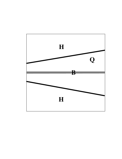
FIG. 1.:

This figure shows a portion of the overdense shock region. Q and H denote QGP and hadronic phases respectively and solid lines denote the interfaces separating the two phases. Shaded region, marked as B, denotes resulting sheet like baryon inhomogeneity.

FIG. 2.:

These figures show plots of baryon density $n_{b}^{q}$ in the QGP phase inside the wake, as a function of time. $\Sigma_{h}$ here is 10^-1. Top figure is for $T_{c}=150$ MeV and bottom figure is for $T_{c}=170$ MeV. Here and in Fig.3, $n_{b}^{q}$ is in fm^-3, while time is given in $\mu s$.

FIG. 3.:

Plots of $n_{b}^{q}$ as a function of time. $\Sigma_{h}$ here is 10^-3. Top figure is for $T_{c}=150$ MeV and the bottom figure is for $T_{c}=170$ MeV.

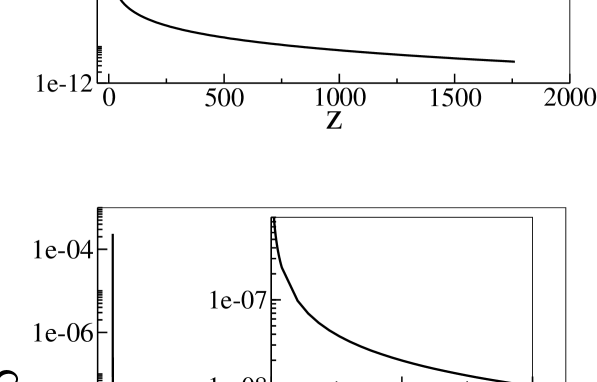
FIG. 4.:

These figures show profiles of baryon inhomogeneities $\rho(z)$ generated by collapsing planar interfaces. $\Sigma_{h}$ here is 10^-1. Top figure is for $T_{c}=150$ MeV and the bottom figure is for $T_{c}=170$ MeV. Here, and in Fig.5, $\rho$ is in units of fm^-3 while $z$ is given in meters. Insets show expanded plots of the region where $\rho$ becomes larger than 1000 times the asymptotic value. We have estimated the error in numerical evaluation of $\rho(z)$ (here, and in Fig.5). Largest error is about 20 % and occurs where wiggles are seen in Fig.5. At other parts of plots, error remains below about 5%.

FIG. 5.:

Plots of $\rho(z)$ vs. $z$ for the case when $\Sigma_{h}$ is 10^-3. Top figure is for $T_{c}=150$ MeV and the bottom figure is for $T_{c}=170$ MeV.

REFERENCES

- [1] H. Kurki-Suonio and E. Sihvola, Phys. Rev. D63, 083508 (2001).
- [2] K. Kainulainen, H. Kurki-Suonio, and E. Sihvola, Phys. Rev. D59, 083505 (1999).
- [3] J.H. Applegate, C.J. Hogan, and R.J. Scherrer, Phys. Rev. D35, 1151 (1987); A. Heckler and C.J. Hogan, Phy. Rev. D47, 4256 (1993);
- [4] K. Jedamzik and G.M. Fuller, Astrophys. J. 423, 33 (1994).
- [5] B. Layek, S. Sanyal, A. M. Srivastava. Phys. Rev. D63, 083512 (2001).
- [6] M.B. Christiansen and J. Madsen, Phys. Rev. D53, 5446 (1996).
- [7] J. Ignatius and D.J. Schwarz, Phys. Rev. Lett. 86, 2216 (2001).
- [8] A.Vilenkin and E.P.S.Shellard, “Cosmic Strings and Other Topological Defects”, (Cambridge University Press, Cambridge, 1994). L. Perivolaropoulos, astro-ph/9410097.
- [9] For reviews, see, S. Sarkar, astro-ph/0205116, K. A. Olive, astro-ph/0202486 .
- [10] R. Durrer, astro-ph/0003363; C.R. Contaldi, astro-ph/0005115; L. Pogosian, Int. J. Mod. Phys. A16S1C, 1043 (2001).
- [11] A. Albrecht, astro-ph/0009129.
- [12] B. Layek, S. Sanyal, A. M. Srivastava, hep-ph/0107174.
- [13] J.R. Gott III, Astrophys. J. 288, 422 (1985); W.A. Hiscock, Phys. Rev. D31, 3288 (1985).
- [14] D.V. Gal’tsov and E. Masar, Class. Quant. Grav.6, 1313, (1989)
- [15] A. Sornborger, Phys. Rev. D56, 6139 (1997).
- [16] A. Stebbins, S. Veeraraghavan, R. Brandenberger, J. Silk, and N. Turok, Astrophys. J. 322, 1 (1987).
- [17] N. Deruelle and B. Linet, Class. Quant. Grav. 5, 55 (1988).
- [18] W.A. Hiscock and J.B. Lail, Phys. Rev. D37, 869 (1988).
- [19] D.P. Bennett and F.R. Bouchet, Phys. Rev. D41, 2408 (1990).
- [20] E. Witten, Phys. Rev. D30, 272 (1984).
- [21] B. Kampfer, Annalen Phys. 9, 605 (2000); S. A. Bonometto, Phys. Rep. 228, 175 (1993).
- [22] G.M. Fuller, G.J. Mathews, and C.R. Alcock, Phys. Rev. D37, 1380 (1988).
- [23] K. Kajantie, Phys. Lett. B285, 331 (1992).
- [24] K. Kajantie and H. Kurki-Suonio, Phys. Rev. D34, 1719 (1986); J. Ignatius, K. Kajantie, H. Kurki-Suonio, and M. Laine, Phys. Rev. D50, 3738 (1994).
- [25] B. Beinlich, F. Karsch, and A. Peikert, Phys. Lett. B390, 268 (1997).
- [26] B. Banerjee and R. V. Gavai, Phys. Lett. B293, 157 (1992).
- [27] P.J.E. Peebles, The large-scale structure of the universe, (Princeton University Press, Princeton, NJ, 1980); T. Padmanabhan, Structure formation in the universe, (Cambridge University Press, Cambridge, 1993); L. Landau and E. Lifshitz, Fluid Mechanics (Pergamon Press Ltd., London, 1959).
- [28] B. Allen and E.P.S. Shellard, Phys. Rev. Lett. 64, 119 (1990).
- [29] E.W. Kolb and M.S. Turner, “The Early Universe”, (Addison-Wesley, Redwood City, California, 1990).
- [30] K. Sumiyoshi, T. Kajino, C.R. Alcock and G.J. Mathews, Phys. Rev. D42,3963 (1990)