Time-Evolution of Collective Meson Fields and Amplification of Quantum Meson Modes in Chiral Phase Transition

Abstract

The time evolution of quantum meson fields in the O(4) linear sigma model is investigated in a context of the dynamical chiral phase transition. It is shown that amplitudes of quantum pion modes are amplified due to both mechanisms of a parametric resonance and a resonance by the forced oscillation according to the small oscillation of the chiral condensate in the late time of chiral phase transition.

1 Introduction

One of the recent interests associated with the physics of the relativistic heavy-ion collisions is to study the dynamics of matter at very high energy density. Especially, it is interesting to investigate the dynamics of the chiral phase transition in connection with the problem of the formation of a disoriented chiral condensate (DCC). In Fig.1, the schematic diagram of the chiral phase transition is depicted in the $O(4)$ linear sigma model.

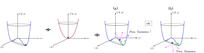
Figure 1: A schematic diagram of the chiral phase transition. The role-down of the condensate is realized in (a). The collective isospin rotation is realized in (b).

In order to investigate the time-evolution of the order parameter and of the fluctuation modes around it in the chiral phase transition, we have formulated the time-dependent variational approach to dynamics of quantum fields in terms of a squeezed state or a Gaussian wave functional[1]. The main advantage of this approach to the dynamical problem lies in the fact that both the degrees of freedom of the mean field and the quantum fluctuations can be treated self-consistently. By using the above-mentioned method, we investigated the dynamics of a collective isospin rotation of quantum meson fields corresponding to the situation which is schematically drawn in Fig.1(b) in the $O(4)$-linear sigma model[1]. We concluded that the collisionless dissipation occurs and we obtained that the damping time is about 40 fm/$c$ for the energy density (160 MeV)⁴. Further, the number of emitted mesons is estimated, which is about 15 pions per fm/$c$ in this dissipative process[1].

In this paper, it is assumed that the chiral phase transition occurs by the rolling down of the chiral condensate in what is called quench scenario, which is schematically depicted in Fig.1(a). The time evolution of chiral phase transition is investigated in this situation. In the early time of this process, the spinodal decomposition may occur. On the other hand, it is interesting in this paper to the mechanism of the chiral phase transition in the late time. Many authors pointed out that the parametric amplification of pion modes with low momenta is realized[2, 3], which leads to the pion emission. Here, we will point out that the resonance mechanism due to forced oscillation is also realized as well as the parametric resonance.

2 Parametric Resonance versus Forced Oscillation

Let us start with the following Hamiltonian density of the $O(4)$ linear sigma model :

$$\mathcal{H}=\frac{1}{2}\pi_{a}({\mbox{\boldmath$x$}})^{2}+\frac{1}{2}\nabla\phi_{a}({\mbox{\boldmath$x$}})\cdot\nabla\phi_{a}({\mbox{\boldmath$x$}})+\lambda\left(\phi_{a}({\mbox{\boldmath$x$}})^{2}-{m^{2}}/{4\lambda}\right)^{2}-H\phi_{0}({\mbox{\boldmath$x$}}).$$ (1)

The squeezed state is adopted as a trial state in the time-dependent variational principle :

$$|{\Phi(t)}\rangle=N\exp\left(i({\overline{\pi}}\!\cdot\!\phi-{\overline{\varphi}}\!\cdot\!\pi)\right)\exp(\phi\cdot\![-(G^{-1}-G^{(0)}{}^{-1})/4+i\Sigma]\!\cdot\!\phi)|{0}\rangle,\quad$$ (2)

where $N$ represents a normalization factor and ${\overline{\pi}}\cdot\phi=\sum_{a=0}^{3}\int\!d^{3}\!{\mbox{\boldmath$x$}}{\overline{\pi}}_{a}({\mbox{\boldmath$x$}},t)\phi_{a}({\mbox{\boldmath$x$}})$ and $\phi\cdot G^{-1}\cdot\phi=\sum_{a=0}^{3}\int\!\int\!d^{3}\!{\mbox{\boldmath$x$}}d^{3}\!{\mbox{\boldmath$y$}}\phi_{a}({\mbox{\boldmath$x$}})G_{a}^{-1}({\mbox{\boldmath$x$}},{\mbox{\boldmath$y$}},t)\phi_{a}({\mbox{\boldmath$y$}})$ and so on. Here, $G^{(0)}_{a}=\langle{0}|\phi_{a}({\mbox{\boldmath$x$}})\phi_{a}({\mbox{\boldmath$y$}})|{0}\rangle$. The expectation values of the field operators are obtained as, for example, $\langle{\Phi(t)}|\phi_{a}({\mbox{\boldmath$x$}})|{\Phi(t)}\rangle={\overline{\varphi}}_{a}({\mbox{\boldmath$x$}},t)$ and $\langle{\Phi(t)}|\phi_{a}({\mbox{\boldmath$x$}})\phi_{a}({\mbox{\boldmath$y$}})|{\Phi(t)}\rangle=$${\overline{\varphi}}_{a}({\mbox{\boldmath$x$}},t){\overline{\varphi}}_{a}({\mbox{\boldmath$y$}},t)+G_{a}({\mbox{\boldmath$x$}},{\mbox{\boldmath$y$}},t)$. Thus, ${\overline{\varphi}}_{a}({\mbox{\boldmath$x$}},y)$ and $G_{a}({\mbox{\boldmath$x$}},{\mbox{\boldmath$y$}},t)$ represent the mean field and the fluctuation around it, respectively. The two-point function $G_{a}({\mbox{\boldmath$x$}},{\mbox{\boldmath$y$}},t)$ can be further expanded in terms of the mode functions under the assumption of the translational invariance : $G_{a}({\mbox{\boldmath$x$}},{\mbox{\boldmath$y$}},t)=\int_{\bf k}e^{i{\bf k}\cdot({\bf x}-{\bf y})}\eta_{\bf k}^{a}(t)^{2}$, where $\int_{\bf k}=\int d^{3}{\bf k}/{(2\pi)^{3}}$. The time-dependence of these functions, together with ${\overline{\pi}}_{a}$ and $\Sigma_{a}$, are determined in the time-dependent variational principle which can be expressed as $\delta\int_{t_{1}}^{t_{2}}dt\langle{\Phi(t)}|i{\partial}/{\partial t}-{\hat{H}}|{\Phi(t)}\rangle=0$, where ${\hat{H}}=\int d^{3}{\mbox{\boldmath$x$}}\ {\mathcal{H}}$.

The equations of motion for the condensate ${\overline{\varphi}}_{a}(t)$ and the fluctuation modes $\eta_{\bf k}^{a}(t)$ under the translational invariance can be expressed as

$${\ddot{\overline{\varphi}}}_{a}(t)-m^{2}{\overline{\varphi}}_{a}(t)+4\lambda{\overline{\varphi}}_{a}(t)^{3}+12\lambda\int_{\bf k}\eta_{\bf k}^{a}(t)^{2}\cdot{\overline{\varphi}}_{a}(t)$$

$$\qquad\qquad\qquad+4\lambda\sum_{b\neq a}\left({\overline{\varphi}}_{b}(t)^{2}+\int_{\bf k}\eta_{\bf k}^{b}(t)^{2}\right){\overline{\varphi}}_{a}(t)-H\delta_{a0}=0\ ,$$

$${\ddot{\eta}}_{\bf k}^{a}(t)+\biggl{[}{\mbox{\boldmath$k$}}^{2}-m^{2}+12\lambda{\overline{\varphi}}_{a}(t)^{2}+12\lambda\int_{{\bf k}^{\prime}}\eta_{{\bf k}^{\prime}}^{a}(t)^{2}$$

$$\qquad\qquad\qquad+4\lambda\sum_{b\neq a}\left({\overline{\varphi}}_{b}(t)^{2}+\int_{{\bf k}^{\prime}}\eta_{{\bf k}^{\prime}}^{b}(t)^{2}\right)\biggl{]}\eta_{\bf k}^{a}(t)-{1}/{4\eta_{\bf k}^{a}(t)^{3}}=0\ .\qquad$$ (3)

Figure 2: The time-evolutions of the mean field (left) and the lowest (middle) and the second excited pion modes (right).

The time-evolution of the mean field[4], i.e., the chiral condensate with the direction of the sigma field, is depicted in the left in Fig.2. The relaxation to the vacuum value is seen due to the inclusion of the quantum fluctuation modes. If we do not take into account the quantum fluctuation modes fully, the relaxation is not seen. Thus, we conclude that the quantum fluctuation modes play an important role in this relaxation process. Also, the amplification of the amplitudes of quantum fluctuation modes with low momenta in the direction of pion fields occurs accompanying with the relaxation of the chiral order parameter[4], which is seen in the middle and the right figures in Fig.2. This phenomena may be understood in terms of a parametric amplification as was mentioned by many authors. However, there is another possibility to amplify the fluctuation modes[5].

In the late time of the chiral phase transition, the dynamical variables can be expanded around the static configurations. Namely, ${\overline{\varphi}}_{0}(t)=\varphi_{0}+\delta\varphi(t)$ and $\eta_{\bf k}^{a}(t)=\eta_{\bf k}^{a}+\delta\eta_{\bf k}^{a}(t)$, where $\varphi_{0}$ and $\eta_{\bf k}^{a}$ are static solutions of (2). In this expansion, we assume that ${|\delta\varphi(t)|}/{\varphi_{0}}\ll 1$ and $|\delta\eta_{\bf k}^{a}(t)/\eta_{\bf k}^{a}|\ll 1$. Then we obtain the approximate equations of motion for the condensate and fluctuation modes as

$$\delta{\ddot{\varphi}}(t)+M_{\sigma}^{2}\delta\varphi(t)=0\ ,\quad\hbox{\rm i.e.,}\quad\delta\varphi(t)=\delta\sigma\cos(M_{\sigma}t)\ ,$$ (4)

$$\delta{\ddot{\eta}}_{\bf k}^{\sigma}(t)+\left[4({\mbox{\boldmath$k$}}^{2}+M_{\sigma}^{2})+24\lambda\varphi_{0}\delta\varphi(t)\right]\delta\eta_{\bf k}^{\sigma}(t)=-24\lambda\eta_{\bf k}^{\sigma}\varphi_{0}\delta\varphi(t)\ ,$$

$$\delta{\ddot{\eta}}_{\bf k}^{\pi}(t)+\left[4({\mbox{\boldmath$k$}}^{2}+M_{\pi}^{2})+8\lambda\varphi_{0}\delta\varphi(t)\right]\delta\eta_{\bf k}^{\pi}(t)=-8\lambda\eta_{\bf k}^{\pi}\varphi_{0}\delta\varphi(t)\ ,$$ (5)

where $\eta_{\bf k}^{0}$ ($\eta_{\bf k}^{i},\ i=1,2,3$) and $\delta\eta_{\bf k}^{0}(t)$ ($\delta\eta_{\bf k}^{i}(t),\ i=1,2,3$) have been rewritten as $\eta_{\bf k}^{\sigma}$ ($\eta_{\bf k}^{\pi}$) and $\delta\eta_{\bf k}^{\sigma}(t)$ ($\delta\eta_{\bf k}^{\pi}(t)$), respectively. Here, $M_{\sigma}$ ($M_{\pi}$) represents the sigma (pi) meson mass in the $O(4)$ linear sigma model, respectively. If the right-hand sides of (5) can be neglected or have no effects, these equations give amplifying solutions in a certain parameter regions due to the parametric resonance mechanism. Actually, the amplitude of the lowest pion mode is amplified as is seen in the middle of Fig.2 in the late time of chiral phase transition. Even if the parametric resonance is not realized, there is another possibility to make amplitudes of meson modes amplify. Actually, the amplitude of the second excited pion mode is amplified due to the forced oscillation mechanism. In our numerical values,

$$\delta{\eta}_{n=2}^{\pi}(t)\approx 0.71(M_{\sigma}/2\sqrt{2M_{\pi}})\cdot(\delta\sigma/\varphi_{0})\cdot t\sin(2\sqrt{{\mbox{\boldmath$k$}}_{2}^{2}+M_{\pi}^{2}}\ t)\ ,$$ (6)

where ${\mbox{\boldmath$k$}}_{2}^{2}=(2\pi/L)^{2}\times 2$ for the second excited mode under the box normalization of the length $L(=\!10$ fm). This behavior is seen in the right of Fig.2.

3 Conclusion

It has been shown approximately and analytically that both the parametric amplification and the resonance due to the forced oscillation occur in the late time of the chiral phase transition. Thus, it is pointed out that there actually coexist two mechanisms to amplify the quantum fluctuation modes in the late time of the chiral phase transition, namely, that a forced oscillation works as well as a parametric resonance.

References

• [1] Y. Tsue, D. Vautherin and T. Matsui, Prog. Theor. Phys. 102 (1999) 313.
Y. Tsue, D. Vautherin and T. Matsui, Phys. Rev. D61 (2000) 076006.
• [2] S. MrΓ³wczyΕ„ski and B. MΓΌller, Phys.Β Lett.Β B363 (1995), 1.
• [3] H. Hiro-Oka and H. Minakata, Phys.Β Rev.Β C61 (2000), 044903.
M. Ishihara, Phys. Rev. C62 (2000), 054908.
S. Maedan, Phys. Lett. B512 (2001), 73.
• [4] Y. Tsue, A. Koike and N. Ikezi, Prog. Theor. Phys. 106 (2001) 807.
• [5] Y. Tsue, Prog. Theor. Phys. 107 (2002) 1285.