The curvaton scenario in supersymmetric theories

Abstract

We analyze the curvaton scenario in the context of supersymmety. Supersymmetric theories contain many scalars, and therefore many curvaton candidates. To obtain a scale invariant perturbation spectrum, the curvaton mass should be small during inflation $m\ll H$. This can be achieved by invoking symmetries, which suppress the soft masses and non-renormalizable terms in the potential. Other constraints on the curvaton model come from nucleosynthesis, gravitino overproduction, and thermal evaporation. The curvaton coupling to matter should be very small to satisfy these constraints (e.g. $h\lesssim 10^{-8}$ for typical soft masses $m\sim\,\mbox{TeV}$).

]

I Introduction

It is now widely believed that the early universe went through a period of superluminal expansion, known as inflation. In addition to explaining the isotropy and homogeneity of our observable universe, inflation can generate the seeds for structure formation. In the usual picture the quantum fluctuations of the slowly rolling inflaton field “freeze in” soon after horizon exit, and become essentially a classical perturbation which remains constant until the moment of horizon re-entry. The produced perturbations only depend on the potential during inflation, and therefore severely constrain possible inflationary models.

Recently there has been a revived interest in the idea that not the perturbations in the inflaton field are responsible for the cosmic microwave background (CMB) fluctuations, but instead isocurvature fluctuations in another scalar field, the “curvaton” field, that is sub-dominant during inflation. After inflation the isocurvature fluctuations of the curvaton field are converted into adiabatic ones. If at decay the contribution of the curvaton to the energy density is considerable, this can lead to perturbations of the observed size. The generation of curvature does not depend on the nature of inflation, beyond the requirement that the Hubble constant must be nearly constant. This mechanism of generating perturbations was first described years ago [1], but it did not attract much interest until recently [2, 3, 4, 5, 6].

The usual set up is the following  : During inflation the curvaton field acquires a large expectation value if it has a negative mass squared, or if its mass is much smaller than the Hubble constant. In the post-inflationary epoch the Hubble expansion acts as a friction term in the equations of motion, and the field remains effectively frozen at a large field value. This stage ends when the Hubble constant becomes of the order of the curvaton mass, $H\sim m_{\phi}$, at which point the curvaton starts oscillating in the quadratic potential. The curvaton behaves as cold matter; its energy density red shifts as $\rho_{\phi}\propto a^{-3}$, with $a$ the scale factor of the universe. After inflaton decay, the universe becomes radiation dominated, with the energy density in radiation red shifting as $\rho_{I}\propto a^{-4}$. During this state of mixed matter, i.e., radiation and cold dark matter, the isocurvature perturbations are transformed into adiabatic ones. The perturbations grow until the curvaton becomes to dominate the universe, or if this never happens, until the curvaton decays.

In this paper we reanalyze the curvaton scenario in the context of supersymmetry (SUSY). SUSY theories contain many scalar fields, and therefore many possible curvaton candidates. However, the finite energy density in the early universe breaks supersymmetry, and induces soft masses of the order of the Hubble constant for all scalar fields [8, 9]. Such heavy fields lead to a perturbation spectrum with a large spectral tilt, in contradiction with observations. Symmetries can be invoked to protect scalars from large soft masses. In D-term inflation Hubble induced soft masses are forbidden by gauge invariance [10]. In no-scale gravity models, and generalizations thereof, there is a Heisenberg symmetry that protects scalar fields from soft mass terms at tree level [11]. Another possibility is that the curvaton field is a (pseudo) Goldstone boson.

Non-renormalizable terms in the potential can lift the flat potential for the large field values needed in the curvaton scenario. For the curvaton model to work such terms should be very small or absent up to some high order. Here SUSY helps, since the non-renormalization theorem assures that operators absent in the superpotential are absent at all scales.

There are several constraints on the curvaton model. The produced perturbations should be adiabatic (which requires that the curvaton decays after inflaton decay), nearly scale invariant (the curvaton mass should be much smaller than the Hubble constant during inflation), and of the correct magnitude. For the perturbations to be sizable, the curvaton energy density needs to be a significant fraction of the total energy density in the universe. To avoid gravitino overproduction the reheat temperature should be sufficiently low. Curvaton decay should not destroy the nucleosynthesis predictions. Furthermore, thermal damping and evaporation should be taken into account.

In the next section we discuss these various constraints on the curvaton model in more detail. In section III we consider the possible (soft) mass terms that can arise in SUSY theories, and analyze the parameter space for the various cases. We end with conclusions.

II Constraints

A Density perturbations

The density perturbations for the curvaton field have been analyzed in [3]. We briefly review their results.

Consider the curvaton with minimal kinetic term and scalar potential $V(\phi)$. We can expand the field in a classical part plus quantum fluctuations

$$\phi({\bf x})=\phi+\delta\phi({\bf x}).$$ (1)

The unperturbed and perturbed curvaton field satisfy respectively

$$\ddot{\phi}+3H_{I}\dot{\phi}+V_{\phi}=0\,,$$ (2)

$$\delta\ddot{\phi}_{k}+3H_{I}\delta\dot{\phi}_{k}+\left(({k}/{a})^{2}+V_{\phi\phi}\right)\delta\phi_{k}=0\,.$$ (3)

Here $\delta\phi_{k}$ are the Fourier components of $\delta\phi$. An overdot denotes $\partial/\partial t$, and a subscript $\phi$ denotes $\partial/\partial\phi$. We have made the first order approximation $\delta(V_{\phi})=V_{\phi\phi}\delta\phi$. The fluctuations of a generic massive scalar field generated during de Sitter stage are then found to be on superhorizon scales (where the gradient term in Eq. (3) is negligible)

$$|\delta\phi_{k}|\simeq\frac{H_{*}}{2k^{3}}\left(\frac{k}{aH_{*}}\right)^{3/2-\nu_{\phi}},$$ (4)

where the subscript $*$ denotes the time of horizon exit. Further, $\nu_{\phi}=(9/4-m/H^{2})$. For $\eta_{\phi}=(m/3H^{2})\ll 1$ one has $3/2-\nu_{\phi}\simeq\eta_{\phi}$ and the spectrum is nearly scale invariant. To be more precise, the spectral tilt of the perturbation is given by

$$n_{\phi}\equiv\frac{d\ln{\mathcal{P}}_{\phi}}{d\ln k}=2\eta_{\phi}-2\epsilon_{H},$$ (5)

and it is assumed that $\epsilon_{H}\equiv\dot{H}/H\ll 1$.

The field remains overdamped until $H\sim m$ when the field starts oscillating in the potential. The potential rapidly approaches a quadratic form, after which the fractional perturbation $\delta\phi/\phi$ remains constant. We parameterize the change in fractional density between the end of inflation and the moment the potential approaches a quadratic form by the parameter $q$:

$$\left(\frac{\delta\phi}{\phi}\right)_{\!{\rm osc}}=q\left(\frac{\delta\phi}{\phi}\right)_{*},$$ (6)

where the subscript osc denotes the quantity at the onset of oscillations, when $H\sim m$. For a quadratic or flat potential the evolution Eqs. (2, 3) for $\phi$ and $\delta\phi$ are the same and $q=1$.

The oscillating curvaton field behaves as non-relativistic matter. After inflaton decay, the energy density becomes a mixture of radiation and matter, and isocurvature perturbation are transformed into adiabatic ones. This period ends when the curvaton becomes to dominate the energy density or, if that never happens, when it decays.

The prediction of the curvaton model for the curvature perturbation can be written as (for small $\eta_{\phi}$):

$${\mathcal{P}}_{\zeta}^{1/2}=\frac{r_{\rm dec}q}{3\pi}\frac{H_{*}}{\phi_{*}},$$ (7)

where the subscript dec means the corresponding quantity evaluated at the time of $\phi$-decay, i.e., when $H\sim\Gamma_{\phi}$. Furthermore, we have defined the parameter $r$ as the ratio of energy density in the curvaton field to the total energy density in the universe $r=\rho_{\phi}/\rho$. The COBE data requires

$${\mathcal{P}}_{\zeta}^{1/2}({\rm COBE}) =4.8\times 10^{-5},$$ (8)

$$n({\rm COBE}) =0.93\pm 0.13.$$ (9)

Moreover, the non-detection of tensor perturbations sets an upper limit on the energy density during inflation

$$H_{*}\lesssim 10^{14}\,\mbox{GeV}.$$ (10)

B Initial conditions

The initial field value of the curvaton at the beginning of inflation is a free parameter. The only constraint is that the energy density in the curvaton field is sub-dominant. The inflaton energy density is $\rho_{I}\sim H_{I}^{2}M_{\rm P}^{2}$, with $H_{I}$ the Hubble constant during inflation. This means that for masses $m^{2}\ll H_{I}^{2}$ a typical initial field value will be large $\phi\gg M_{\rm P}$.

We consider scalar potentials of the form

$$V(\phi)=\frac{1}{2}m^{2}\phi^{2}+\frac{\lambda}{M^{n}}\phi^{4+n}.$$ (11)

The non-renormalizable operators, suppressed by the Planck scale or some other ultraviolet cutoff, will generate an effective mass $\delta m_{\rm HO}^{2}=\partial^{2}V/\partial\phi^{2}\equiv V_{\phi\phi}>H$ for large initial field values. The curvaton is underdamped, and decreases exponentially fast.

The effective mass squared term during inflation can be positive or negative. The finite energy density in the early universe breaks supersymmetry. This leads to soft mass terms of the form $m^{2}=cH_{I}^{2}$. The sign of $c$ is determined by the Kähler potential.

If the effective mass squared is negative and the initial curvature amplitude is large, the curvaton field will approach its minimum exponentially fast. If on the other hand, the curvaton is initially at the origin, or at some small field value, the field is highly damped. It will approach the minimum at a rate $\phi\propto m^{2}t$ (for constant $m$). At $t\sim H_{I}/m^{2}$ the motion goes non-linear and the classical field reaches the minimum exponentially fast. We will assume that inflation last sufficiently long for the field to be in its minimum.

If the mass squared is positive during inflation, and the field has large initial values, it will decrease exponentially fast until $m\lesssim H_{I}$, and the field becomes overdamped. The field value typically freezes at $\phi\sim H_{I}$. After that, the field decreases only linearly until the classical motion becomes non-linear at $t\sim H_{I}/m^{2}$. Quantum fluctuations grow during inflation as $\langle\phi^{2}\rangle\approx H_{I}^{3}t/4\pi^{2}$ until they reach at $t\sim H_{I}/m^{2}$ a saturation value [12]

$$\langle\phi^{2}\rangle\approx\frac{3}{8\pi^{2}}\frac{H_{I}^{4}}{m^{2}},$$ (12)

with coherence length (provided the classical field has a small amplitude, $\phi\ll H_{I}/m$)

$$l\sim H_{I}^{-1}\exp\left(\frac{3H_{I}^{2}}{2m^{2}}\right).$$ (13)

The low momentum modes of these fluctuations will be indistinguishable from a classical field with an amplitude $\phi_{I}\approx\sqrt{\langle\phi^{2}\rangle}$. For the field to be homogeneous on the current horizon size $m^{2}/H_{I}^{2}<1/40$. If higher order terms in the potential are non-negligible, $m^{2}$ should be replaced by $\delta m_{\rm HO}^{2}=V_{\phi\phi}$ in the above formulas.

C Domination

When $H\sim m$ the curvaton field start oscillating in its potential; it behaves as cold dark matter with $\rho_{\phi}\propto a^{-3}$. After inflaton decay the universe becomes radiation dominated, its energy density red shifting as $a^{-4}$. The fractional energy density in the curvaton field increases until a maximum value at curvaton decay:

$$r_{\rm dec}=\left(\frac{\rho_{\phi}}{\rho}\right)_{\rm dec}\sim\frac{1}{h}\frac{\phi_{\rm osc}^{2}}{M_{\rm P}^{2}}\left(\frac{\Gamma_{I}}{m}\right)^{\alpha},$$ (14)

with $\alpha=0$ for $\Gamma_{I}>m$, and $\alpha=1/2$ for $\Gamma_{I}<m$. We have assumed instant reheating, with reheating temperature $T\sim g_{*}^{1/4}\sqrt{M_{\rm P}\Gamma_{I}}$. Above $T\sim 10^{-1}\,\mbox{GeV}$ the effective degrees of freedom $g_{*}={\mathcal{O}}(100)$, whereas round MeV temperatures it drops to $g_{*}={\mathcal{O}}(10)$. Further, we used $\Gamma_{\phi}\sim h^{2}m$, with $h$ the coupling, yukawa or gauge, of the curvaton to matter. The curvaton field dominates the energy density in the universe at decay for $r\gtrsim 1/2$.

As can be seen from Eq. (14), to avoid a period of curvaton dominated inflation, the curvaton cannot dominate the energy density before the onset of oscillation. This translates into

$$\phi_{\rm osc}<M_{\rm P}.$$ (15)

D Thermal constraints

The curvaton field must decay before $T\sim\,\mbox{MeV}$, to not destroy the successful predictions of nucleosynthesis. This gives

$$\Gamma_{\phi}\sim h^{2}m_{\phi}\gtrsim 10^{-25}\,\mbox{GeV}.$$ (16)

The reheat temperature of the universe after inflaton decay cannot be too high; to avoid gravitino overproduction requires $T_{I}<10^{6}-10^{9}\,\mbox{GeV}$. However, gravitinos produced by inflaton decay are diluted by the entropy generated in the curvaton decay. If the curvaton has a sub-dominant energy density at decay the dilution is negligible. The dilution factor $\Delta\equiv s_{\rm after}/s_{\rm before}$ is

$$\Delta=\frac{1}{h}\frac{\phi_{\rm osc}^{2}}{M_{\rm P}^{2}}\left(\frac{\Gamma_{I}}{m}\right)^{\alpha}$$ (17)

This implies $T_{I}<\Delta(10^{6}-10^{9})\,\mbox{GeV}$, or

$$\Gamma_{\phi}\lesssim(10^{-7}-10^{-1})\,\mbox{GeV}\left(\frac{\phi_{\rm osc}}{M_{\rm P}}\right)^{4}\left(\frac{m}{\Gamma_{I}}\right)^{1-2\alpha}.$$ (18)

Similarly, any preexisting baryon asymmetry gets diluted by the entropy production. Therefore, if $\Delta>10^{10}$, the baryon asymmetry must be generated in the out-of-equilibrium curvaton decay, or at lower temperatures.

Finite temperature effects can lead to thermal damping or early thermal decay of the condensate [13, 14]. Large thermal masses $\delta M_{th}\gtrsim H>m$ may induce early oscillations, which reduces the energy stored in the condensate. When the temperature is higher than the effective mass of the particles coupled to the condensate, i.e., $T\gtrsim h\phi$, the curvaton receives a thermal mass $\delta M_{\rm th}^{2}=(1/4)h^{2}T^{2}$. For lower temperatures $T\lesssim h\phi$ the running of the yukawas is modified leading to an effective thermal mass $M_{\rm th}=h^{4}T^{4}/\phi^{2}$. Thermal damping is unimportant when

$$\frac{\delta M_{\rm th}^{2}}{H^{2}}\lesssim 1\quad{\rm for}\;\;H>m$$ (19)

It is important to note that even before $H\sim\Gamma_{I}$ there is a dilute plasma with temperature $T\sim(T_{I}^{2}M_{\rm P}H)^{1/4}$ [15].

Another effect to be considered is thermal evaporation by particles which are in equilibrium with the thermal bath, that is for which $m_{\rm eff}\sim h\phi<T$ [14]. For a coupling in the scalar potenital $V\ni h\phi^{2}\chi^{2}$ the cross section for $\phi\chi$-scattering is $\sigma\sim h^{2}/E_{\rm cm}^{2}$. The typical center of mass energy is $E_{\rm cm}\sim\sqrt{Tm}$, the mean of the typical $\chi$-energy ($\sim T$) and $\phi$-energy ($\sim m$). The thermal decay rate is $\Gamma_{\rm th}\sim\sigma T^{3}\sim h^{2}T^{2}/m$. If the condensate evaporates thermally when $H\gtrsim\Gamma_{I}$, the isocurvature curvaton are not converted into adiabatic perturbations, and the curvaton scenario does not work. This happens when

$$\Gamma_{\rm th}\gtrsim H\quad\&\quad T>h\phi.$$ (20)

All thermal constraints can be circumvented if the inflaton sector and curvaton sector decouple completely, as is proposed in reference [6]. In their scenario the inflaton is a hidden sector field which decays into hidden sector radiation, while the curvaton field is responsible for reheating of the MSSM sector. Then, before curvaton decay there is no thermal bath of MSSM particles, and thermal effects are negligibly small.

III Various models

The finite energy density in the early universe breaks supersymmetry, leading to soft masses in the scalar potential which are generically of the order $H$ [8]. Soft mass terms are both induced by non-renormalizable as by supergravity corrections. In global SUSY, non-renormalizeble terms in the Kähler potential of the form $\delta K=\int{\rm d}^{4}\theta\,M_{\rm P}^{-2}\phi^{\dagger}\phi I^{\dagger}I$ lead to mass terms $\delta m^{2}\sim(\rho/M_{\rm P}^{2})\sim H^{2}$. Supergravity corrections to the Lagrangian likewise induce mass terms of the order $H^{2}$. The mass squared can be either positive or negative, depending on the specific Kähler potential.

However, the curvaton scenario cannot work for $|\delta m|={\mathcal{O}}(H)$, since this would give large deviations from scale dependence in the density fluctuations, in conflict with observations. The COBE requirement Eqs. (5, 9) translates into $m/H_{I}<10$. But the constraint can be made stronger. For a positive mass squared a large coherence length for the fluctuations is needed, which requires $m/H_{I}<1/40$. For a negative mass squared, there is another bound. After horizon exit the zero mode and fluctuations evolve according to Eqs. (2, 3). Since the mass is negative $m^{2}=-cH^{2}$, the classical field is at its minimum. Substituting this in the equation for the fluctuations yields a positive effective mass squared $m_{\rm eff}^{2}=[(n+4)(n+3)-1]cH^{2}$. When the effective mass is of the order $H$ damping is efficient, and the fluctuations will decrease exponentially fast during the last 60 e-folds of inflation. This gives a bound $m/H_{I}\lesssim 1/60$.

Therefore, for the curvaton scenario to work within the context of supersymmetry we need to invoke symmetries to protect the scalar field from obtaining large soft masses.

When inflation is driven by $D$-terms, gauge invariance forbids the appearance of soft masses for the scalar fields [10]. The scalar mass are set by the low energy SUSY breaking, and are typically of the order $\sim m_{3/2}$. At the end of inflation, the vacuum energy density stored in $D$-terms is transferred to kinetic and $F$-terms, which do induce mass terms of the $\delta m^{2}\sim H^{2}$. The sign of the mass term depends on the Kähler potential.

No-scale type gravity models possess an extra, so-called Heisenberg symmetry, which forbids soft mass terms at tree level [11]. Masses are induced radiatively, and are suppressed by loop factors

$$\delta m^{2}\sim\frac{c}{4\pi^{2}}h^{2}H^{2},$$ (21)

with $c={\mathcal{O}}(1)$, which can be positive or negative depending on whether gauge or yukawa coupling dominate, and on which field (hidden sector, matter field, dilaton) is the inflaton. For $|\delta m^{2}|>m^{2}$, where the curvaton mass is typically set by low energy SUSY breaking, the mass squared can be negative during inflation. Since the gravitino mass decouples in no-scale gravity, there is no problem related to gravitino overproduction.

Pseudo-Goldstone bosons are protected from soft corrections; the mass is set by the breaking scale of the global symmetry. The analysis for this case is, apart from constraints concerning gravitino production, the same as for standard model curvaton fields.

A Negative mass squared — no-scale inflation

In this section we consider the parameter space for curvaton fields with no-scale type masses of the form

$$\delta m^{2}\sim-10^{-2}h^{2}H^{2}.$$ (22)

For the induced mass to be the dominant term, we also require that during inflation the effective mass is negative, i.e.,

$$m^{2}<|\delta m^{2}|$$ (23)

Then during inflation the $\phi$-field is driven to its classical minimum

$$\phi_{\rm min}\sim(H^{2}M^{n}/\lambda)^{1/(n+2)}.$$ (24)

In the post-inflationary evolution the field keeps tracking its instantaneous minimum until $|\delta m^{2}|\sim m^{2}$, at which point the mass becomes positive, and the field freezes until $H\sim m$. The higher order terms in the potential Eq. (11) are of the same order as the mass term at the minimum, and therefore do not alter the conclusion that the fluctuation spectrum Eq. (5) is flat. However, the higher order terms are important for the evolution of the fluctuations. With the classical field at its minimum, it follows from Eq. (3) that the fluctuations have a positive effective mass squared $m_{\rm fluc}^{2}=+\left[(n+4)(n+3)-1\right]10^{-2}h^{2}H^{2}$. While the zero mode decreases for $|\delta m|>m$, fluctuations are overdamped and remain frozen. This leads to a $q$-factor Eq. (6)

$$q=\frac{\phi_{*}}{\phi_{\rm osc}},$$ (25)

with $\phi_{\rm osc}$ the classical minimum Eq. (24) at $|\delta m|\approx 0.1hH\sim m$. The fraction of energy density stored in the curvaton field at decay is

$$r_{\rm dec}=\frac{1}{h}\frac{\phi_{\rm osc}^{2}}{M_{\rm P}^{2}}\left(\frac{\Gamma_{I}}{m}\right)^{\alpha}.$$ (26)

The CMB constraint Eqs. (7, 9) then reads

$$\frac{H_{*}}{h}\left(\frac{m^{2}M^{n}}{\lambda}\right)^{\frac{1}{n+2}}\left(\frac{\Gamma_{I}}{m}\right)^{\alpha}=3\times 10^{33}\,\mbox{GeV}^{2}.$$ (27)

Domination occurs for $r\sim 1$, or

$$h\lesssim\left(\frac{m}{M_{\rm P}}\right)^{4/(n+2)}$$ (28)

The curvaton scenario does not work with at quartic term in the potential. The CMB constraint for $n=0$, together with bound on the Hubble constant during inflation Eq. (10) and nucleosynthesis constraints Eq. (16) eliminates all parameter space.

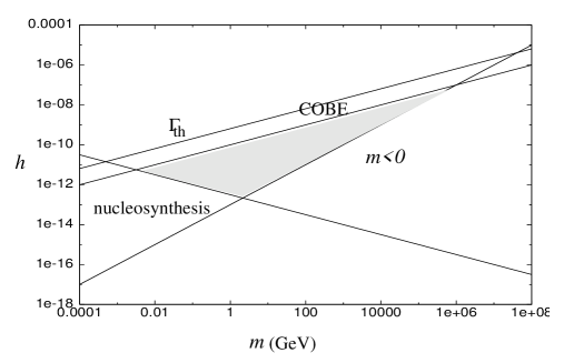
FIG. 1.: Parameter space for the curvaton model in no-scale type gravities with a soft mass term $\delta m^{2}\approx-10^{-2}h^{2}H^{2}$ during inflation, for the parameters $M/\sqrt{\lambda}=M_{\rm P}^{\prime}$, $n=2$, and $\Gamma_{I}>m$. The curvaton scenario works for masses and couplings in the shaded area.

If the potential if lifted by a $\phi^{6}$-term, the CMB constraint becomes

$$h<10^{-8}\left(\frac{H}{10^{14}\,\mbox{GeV}}\right)\left(\frac{m}{10^{4}\,\mbox{GeV}}\frac{M/\sqrt{\lambda}}{M_{\rm P}}\right)^{1/2}\left(\frac{\Gamma_{I}}{m}\right)^{\!-\alpha}$$ (29)

This bound is shown in Fig. 1 for $M/\sqrt{\lambda}=M_{\rm P}$ and $\Gamma_{I}>m$ ($\alpha=0$), together with the constrains coming from nucleosynthesis, the requirement of having a negative effective mass during inflation Eq. (23), and from thermal evaporation Eq. (20).

If the condensate evaporates thermally when $H\gtrsim\Gamma_{I}$, no adiabatic perturbations are generated, and the curvaton scenario fails. The bound is strongest in the thermal plasma after inflaton decay, for $H\lesssim\Gamma_{I}$. From Eq. (20) it then follows that thermal evaporation occurs for couplings in the range

$$10^{-9}\left(\frac{m}{\,\mbox{GeV}}\right)^{1/2}<h<1\left(\frac{M_{\rm P}}{M/\sqrt{\lambda}}\right)^{1/2},$$ (30)

In the same coupling range damping by thermal masses can become important.

There are no constraints from gravitino production, as the gravitino mass can be arbitrary high in no-scale models. Further, $\phi_{\rm osc}<M_{\rm P}$ automatically, and therefore $\phi$-driven inflation does not occur Eq. (15)

The $\phi$-field can only act as the curvaton for small masses $m\lesssim 10^{5}\,\mbox{GeV}$ and small couplings $h\lesssim 10^{-8}$. For typical soft masses $m\sim\,\mbox{TeV}$, one needs to fine tune all parameters $H\to 10^{14}\,\mbox{GeV}$, $|\delta m|\to m$, $M/\sqrt{\lambda}>M_{\rm P}$ and $h\to 10^{-7}-10^{-8}$ for the curvaton scenario to work.

For higher order operators $n>2$ the CMB constraint allows for larger values of the coupling. However, not much parameter space opens up as $h$ is bounded from above to avoid early thermal evaporation.

B Positive mass squared — no-scale inflation and Goldstone bosons

In this section we discuss the parameter space for curvaton models with a positive mass squared $0<m^{2}\ll H_{I}^{2}$. Such mass terms can arise in no-scale supergravity, or alternatively the curvaton can be a Goldstone boson. In $D$-term inflation the mass is protected from soft corrections during inflation, but not afterwards; we will discuss this case in the section III D.

For the moment we ignore possible non-renormalizable operators, but we will discuss them in the next subsection. Furthermore, we approximate the Hubble constant as constant during inflation, i.e., we set $H_{*}\approx H_{I}$. Here $H_{*}$ is the Hubble constant when density fluctuations of the size of our present horizon leave the horizon, which happens some 60 e-folds before the end of inflation. $H_{I}$ is the Hubble constant at the end of inflation, which sets the magnitude of the condensate.

During inflation a condensate is formed with magnitude given by Eq. (12). The curvature perturbation is given by Eq. (7) with $q\approx 1$. If the curvaton comes to dominate the universe, $r\approx 1$ (see Eq. (14)), and the COBE constraint becomes

$$h \lesssim 10^{-22}\left(\frac{m^{2}}{\,\mbox{GeV}^{2}}\right)\left(\frac{\Gamma_{I}}{m}\right)^{\alpha}$$ (31)

$$m \approx 10^{-4}H_{I}.$$ (32)

For larger values of the coupling, the curvaton energy density remains sum-dominant. Then $r<1$ and the COBE constraint reads

$$h=10^{-34}\left(\frac{H_{I}^{3}}{m\,\mbox{GeV}^{2}}\right)\left(\frac{\Gamma_{I}}{m}\right)^{\alpha},$$ (33)

$$10^{4}m\lesssim H_{I}\lesssim 10^{14}\,\mbox{GeV}.$$ (34)

For couplings in the range $10^{-9}\sqrt{m/\,\mbox{GeV}}<h<h_{\rm up}$ with

$$h_{\rm up}\sim\left\{\begin{array}[]{*{2}{l}}10^{2}\left(\frac{\Gamma_{I}H\,\mbox{GeV}^{2}}{m^{4}}\right)^{1/4}\left(\frac{\Gamma_{I}}{H}\right)^{\beta/2}&\quad(r\sim 1)\\ 10^{-8}\left(\frac{H^{3}m^{2}}{\,\mbox{GeV}^{5}}\right)^{1/10}\left(\frac{\Gamma_{I}}{m}\right)^{2\alpha/5}\left(\frac{\Gamma_{I}}{H}\right)^{3\beta/20}&\quad(r<1)\\ \end{array}\right.$$ (35)

the condensate is destroyed by thermal scattering before the adiabatic perturbations are generated. Here $\beta=1$ for $H>\Gamma_{I}$, and $\beta=0$ for $H<\Gamma_{I}$. These constraints are plotted in Fig. 2 for the case $\Gamma_{I}>m$. Also shown are the bounds from nucleosynthesis and from $\phi$-dominated inflation Eq. (15). If non-renormalizable terms lift the flat direction at a cutoff scale $\Lambda\lesssim M_{\rm P}$, the constraint $\phi_{\rm osc}\lesssim M_{\rm P}$ is automatically satisfied, and the bound from $\phi$-dominated inflation should be re-interpreted as a cutoff on the validity of the theory: for higher couplings non-renormalizable terms can no longer be neglected.

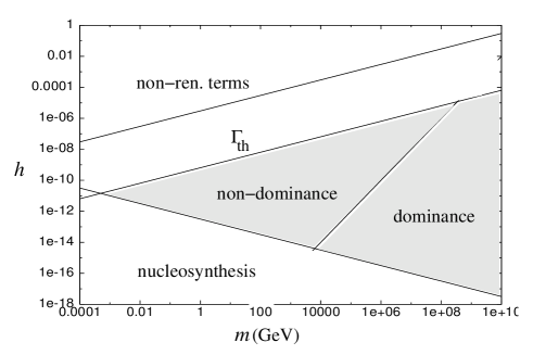
FIG. 2.: Parameter space for models with a positive mass squared during inflation, for $\Gamma_{I}>m$. The curvaton scenario works for masses and couplings in the shaded area.

In the allowed region of parameter space in Fig. 2, the Hubble-induced mass term in no-scale gravities is smaller than the low energy mass: $|\delta m|\sim 10^{-1}hH_{I}<m$. Hence, the exclusion plot based on a constant mass is also applicable to this class of models. As mentioned before, there are no constraints from gravitino overproduction in no-scale gravity, as the gravitino mass can be arbitrary high.

Gravitino production does constrain the Goldstone boson curvaton field. The entropy production from the late-time curvaton decay is suppressed by the small factor $(\phi_{\rm osc}/M_{\rm P})^{4}$ (see Eq. 17). Only for masses close to the upper bound $m\to 10^{-4}H_{I}\sim 10^{10}\,\mbox{GeV}$ can it be significant. For smaller masses the dilution is negligible small, and the only way to avoid gravitino overproduction is to have $T_{I}<10^{6}-10^{9}\,\mbox{GeV}$. This means $\Gamma_{I}<m\>$ ($\alpha=1/2$). Smaller decay rates are needed to get curvaton domination. Furthermore, the constraints from $\phi$-dominated inflation, and from the COBE data Eq. (34) become tighter. This last constraint is equivalent to requiring the curvaton to decay after inflaton decay. The results are plotted in Fig. 3 for $T_{I}=10^{7}\,\mbox{GeV}$.

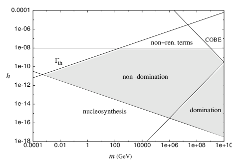
FIG. 3.: Constraints from gravitino production for $T_{I}=10^{7}\,\mbox{GeV}$

C Positive mass squared — non-renormalizable terms

The non-renormalizable terms in the potential Eq. (11) can alter the picture described in the previous subsection. Higher order terms are negligible when $V_{\phi\phi}<m^{2}$ during inflation, that is when

$$m<\left[\sqrt{10^{16}\frac{3}{8\pi^{2}}}\left(\frac{H_{*}/m}{10^{4}}\right)\right]^{(n+2)/2n}.$$ (36)

In the case of curvature domination the COBE data requires $H\sim 10^{4}m$. Taking $M^{n}/\lambda=M_{\rm P}$, it follows that higher order terms are negligible only for small enough masses: $m\lesssim 10^{3}\,\mbox{GeV}$ for $n=2$, $m\lesssim 10^{7}\,\mbox{GeV}$ for $n=4$, and $m\lesssim 10^{8}\,\mbox{GeV}$ for $n=6$. For larger masses the effective mass $m_{\rm eff}^{2}\equiv V_{\phi\phi}$ sets the initial conditions during inflation. As long as $m_{\rm eff}^{2}\ll H_{I}^{2}$ the perturbation are nearly scale invariant and the curvaton scenario is possible. We will analyze this possibility in this subsection.

The effective mass $V_{\phi\phi}$ sets the initial value of the curvaton, which from Eq. (12) is

$$\phi_{I}\sim\left(\frac{3}{8\pi^{2}}\frac{H^{4}M^{n}}{(n+4)(n+3)\lambda}\right)^{\frac{1}{n+4}}.$$ (37)

When $H\sim m_{\rm eff}$ the curvaton field starts oscillating. After a few oscillation the potential approaches a quadratic form. We approximate $q\approx 1$. During the first initial oscillation the curvaton energy density changes as

$$\rho(H)=\frac{m(H)}{m_{(}H_{I})}\left(\frac{a_{0}}{a}\right)^{3}\rho(H_{I}),$$ (38)

where $a$ is the scale factor of the universe. The field amplitude at the onset of quadratic oscillations, when $m(H)=m$, is $\phi_{\rm osc}^{2}=\kappa^{1/2+\alpha}\phi_{I}^{2}$. Here we have parametrized $m=\kappa\sqrt{V_{\phi\phi}}$.

The COBE constraints Eq. (9) for domination $r\sim 1$ translate into

$$\left\{\begin{array}[]{lll}m<10^{4}\,\mbox{GeV}C_{m},\quad h<10^{-16}C_{h}\qquad(n=2)\\ m<10^{7}\,\mbox{GeV}C_{m},\quad h<10^{-8}\;C_{h}\qquad(n=4)\\ m<10^{8}\,\mbox{GeV}C_{m},\quad h<10^{-6}\;C_{h}\qquad(n=6)\\ \end{array}\right.$$ (39)

With $C_{m}=\kappa(M\lambda^{-1/n}/M_{\rm P})$ and $C_{h}=\kappa^{1/2+\alpha}(\Gamma_{I}/m)^{\alpha}$. For the non-domination case $r<1$, the COBE data requires

$$h<\left\{\begin{array}[]{lll}10^{-20}m^{5/4}\kappa^{-3/4+\alpha}\left(\frac{\Gamma_{I}}{m}\right)^{\alpha}\left(\frac{M/\lambda^{1/n}}{M_{\rm P}}\right)^{3/4}&\quad(n=2)\\ 10^{-15}m\kappa^{-1/2+\alpha}\left(\frac{\Gamma_{I}}{m}\right)^{\alpha}\left(\frac{M/\lambda^{1/n}}{M_{\rm P}}\right)&\quad(n=4)\\ 10^{-13}m^{7/8}\kappa^{-3/8+\alpha}\left(\frac{\Gamma_{I}}{m}\right)^{\alpha}\left(\frac{M/\lambda^{1/n}}{M_{\rm P}}\right)^{9/8}&\quad(n=6)\end{array}\right.$$ (40)

And $H_{I}$ is constraint $10^{4}m/\kappa\lesssim H_{I}\lesssim 10^{14}\,\mbox{GeV}$.

The constraints are shown in Fig. 4 for $M^{n}/\lambda=M_{\rm P}^{n}$, $\Gamma_{I}>m$, and $\kappa\to 1$. Note that one can read off from the plot the parameter space where $m^{2}>V_{\phi\phi}$ during inflation and higher order terms can be neglected, namely the region to the left of the COBE constraints. In most of the curvaton dominated region in Fig. 2 the non-normalizable terms cannot be neglected. Curvaton domination can only occur if the non-renormalizable terms are absent to some very high order, or if the effective mass during inflation is set by the higher order terms. This conclusion does not change when $\Gamma_{I}<m$, since both the COBE constraints and the requirement $r\sim 1$ have the same $\Gamma_{I}$ dependence.

For small masses, $m=\kappa\sqrt{V_{\phi\phi}}$ with $k\ll 1$, Fig. 4 indicates the couplings $h$ needed for the curvaton scenario after shifting the plot by some power of $\kappa$ (both to lower $h$ and $m$ values, see Eqs. (39,40)). Taking $\Gamma_{I}<m$, or $M^{n}/\lambda<M_{\rm P}^{n}$ has a similar effects, the COBE bounds shifts to lower couplings and smaller masses.

To summarize, the non-renormalizable terms can be neglected only for sufficiently small masses. But in a large part of parameter space, where the curvaton dominates the energy density, their contribution to the mass term during inflation is dominant, unless these operators are absent to a very high order. If the higher order terms dominate, the curvaton scenario may still work, but smaller couplings and masses are needed.

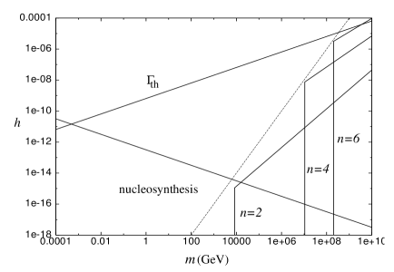
FIG. 4.: Parameter space when the effective mass is set by higher order terms $\phi^{6}$ ($n=2$), $\phi^{8}$ ($n=4$), or $\phi^{10}$ ($n=4$). Here $M=M_{\rm P}$, $\lambda=1$, $\Gamma_{I}>m$, and $\kappa\to 1$. The dashed line corresponds to the $r=1$ line in the absence of higher order terms (from Fig. 2), which is added for comparison.

D D-term inflation

In $D$-term inflation there is no Hubble induced soft mass term during inflation. However at the end of inflation, the energy in $D$-terms is transferred to $F$-terms and kinetic energy and a mass term $m^{2}=cH^{2}$, with $c={\mathcal{O}}(1)$ is induced.

If $c<1$ the field approaches its minimum Eq. (24). The only difference with the no-scale model discussed in section III A is the initial field value $\phi_{*}$. If we ignore the change in $\delta\phi/\phi$ from turning on the Hubble induced mass, then $\phi_{*}$ drops out of the COBE constraint. Therefore the parameter space is given by Fig. 1, with the important difference that the constraint $m_{\rm eff}<0$ of Eq. (23) does not apply.

For $c>1$ the field value decreases at the end of inflation, according to Eq. (38), and $\phi_{\rm osc}\sim(m/H_{\rm end})^{3}\phi_{*}$ (for $\Gamma_{I}<m$) with $H_{\rm end}$ the Hubble value at the end of inflation. Ignoring the change in $\delta\phi/\phi$ from turning on the Hubble induced mass, the only difference with sections III C and III B is that the coupling in the COBE constraints Eqs (32,34) and Eqs (39,40)) should be replaced by $h\to h(m/H_{\rm end})^{3}$. This decreases parameter space, and moves the domination curve to the right.

IV Conclusions

The finite energy density during inflation breaks supersymmetry, and induces soft masses of the order of the Hubble constant for all scalars. The inflationary perturbation spectrum for these fields is highly non-Gaussian, and therefore they cannot play the role of the curvaton. To avoid this conclusion one has to invoke symmetries, to keep the soft mass terms small during inflation.

In no-scale type gravities, scalar masses are induced radiatively and are suppressed to the soft breaking scale ($M_{s}\sim H$) by loop factors. These theories have the additional advantage that the gravitino mass can be arbitrarily large, thereby avoiding problems with gravitino overproduction. In $D$-term inflation gauge symmetry forbids soft Hubble-induced masses. At the end of inflation, when $D$-terms are converted to $F$ terms and kinetic energy, a soft mass term $|\delta m^{2}|\sim H^{2}$ appears. Pseudo-Goldstone bosons are protected from soft mass terms. Their mass is set by the amount of symmetry breaking, and can be small. Apart from constraints considering gravitino production, the analysis for this case also applies to standard model fields.

In all cases the parameter space for the curvaton scenario is constrained by bounds from nucleosynthesis and early thermal evaporation. To avoid thermal evaporation the coupling to matter should be small. In particular, for typical low energy soft masses $m\sim\,\mbox{TeV}$ and an interaction term in the scalar potential of the form $V\ni h\phi^{2}\chi^{2}$, thermal evaporation is negligible for $h\lesssim 10^{-8}$. But we note that thermal constraints can be circumvented if the inflaton and curvaton sector decouple completely [6].

Strong constraints also come from the existence of non-renormalizable operators in the potential, which are suppressed by some cutoff scale $M$. For operators of the form $V\ni\phi^{n+4}/M_{\rm P}^{n}$, the curvaton mass is constraint to $m\lesssim 10^{3}\,\mbox{GeV}$ for $n=2$, $m\lesssim 10^{7}\,\mbox{GeV}$ for $n=4$, and $m\lesssim 10^{8}\,\mbox{GeV}$ for $n=6$. These bounds are absent for $D$-term inflation, with a negative Hubble induced mass squared after inflation.

One can ask whether there are any natural candidates for the curvaton field. Affleck-Dine condensates have masses of the low energy SUSY breaking scale, $m\sim\,\mbox{TeV}$. Along most flat directions the $\phi^{6}$ term is absent. However, couplings to matter are too large, and do not satisfy the curvaton constraint $h<10^{-8}$.

Moduli and polyoni fields have Planck mass suppressed couplings and typically decay after nucleosynthesis. This can be avoided if the mass term is sufficiently high, $m\gtrsim 100\,\mbox{TeV}$. In no-scale gravities this is naturally achieved by giving them a mass of the order of the gravitino mass. But that means that also their mass during inflation is too large ($\delta m^{2}\sim H^{2}$), and they cannot be the curvaton.

Right-handed sneutrinos can have small couplings to matter. In the sea saw model, neutrinos obtain masses $m_{\nu}\sim h\langle H_{u}\rangle/M_{N}\lesssim 10^{-3}\,\mbox{eV}$, where $\langle H_{u}\rangle$ is the expectation value of the Higgs field and $M_{N}$ the sneutrino mass. In [17] leptogenesis from an sneutrino dominated universe is considered. In this model, sneutrino has mass $M_{N}\sim 10^{7}\,\mbox{GeV}$ and $h\lesssim 10^{-12}$. The sneutrino can be the curvaton if there are no constraints from gravitino production. Moreover, if the sneutrino mass is generated at some GUT scale, one needs to explain why $M_{N}\ll M_{GUT}$ and why non-renormalizable operators are absent to very high order.

This work was supported by the European Union under the RTN contract HPRN-CT-2000-00152 Supersymmetry in the Early Universe.

REFERENCES

- [1] S. Mollerach, Phys. Rev. D 42, 313 (1990); A. D. Linde and V. Mukhanov, Phys. Rev. D 56, 535 (1997). [arXiv:astro-ph/9610219].
- [2] K. Enqvist and M. S. Sloth, Nucl. Phys. B 626, 395 (2002) [arXiv:hep-ph/0109214].
- [3] D. H. Lyth and D. Wands, Phys. Lett. B 524, 5 (2002), [arXiv:hep-ph/0110002]; D. H. Lyth, C. Ungarelli and D. Wands, arXiv:astro-ph/0208055.
- [4] T. Moroi and T. Takahashi, Phys. Lett. B 522, 215 (2001) [Erratum-ibid. B 539, 303 (2002)] [arXiv:hep-ph/0110096],
- [5] K. Dimopoulos and D. H. Lyth, arXiv:hep-ph/0209180]; N. Bartolo and A. R. Liddle, Phys. Rev. D 65, 121301 (2002), [arXiv:astro-ph/0203076]; T. Moroi and H. Murayama, arXiv:hep-ph/0211019; T. Moroi and T. Takahashi, arXiv:hep-ph/0210392.
- [6] K. Enqvist, S. Kasuya and A. Mazumdar, arXiv:hep-ph/0211147.
- [7] M. Bastero-Gil, V. Di Clemente and S. F. King, arXiv:hep-ph/0211011.
- [8] M. Dine, W. Fischler and D. Nemeschansky, Phys. Lett. B 136, 169 (1984); O. Bertolami and G. G. Ross, Phys. Lett. B 183, 163 (1987); E. J. Copeland, A. R. Liddle, D. H. Lyth, E. D. Stewart and D. Wands, Phys. Rev. D 49, 6410 (1994), [arXiv:astro-ph/9401011].
- [9] For a discussion of soft mass terms during inflation, see also the review paper by K. Enqvist and A. Mazumdar, arXiv:hep-ph/0209244.
- [10] P. Binetruy and G. R. Dvali, Phys. Lett. B 388, 241 (1996), [arXiv:hep-ph/9606342]; C. F. Kolda and J. March-Russell, Phys. Rev. D 60, 023504 (1999), [arXiv:hep-ph/9802358].
- [11] M. K. Gaillard, H. Murayama and K. A. Olive, Phys. Lett. B 355, 71 (1995), [arXiv:hep-ph/9504307].
- [12] T. S. Bunch and P. C. Davies, Proc. Roy. Soc. Lond. A 360, 117 (1978); A. D. Linde, Phys. Lett. B 116, 335 (1982); A. A. Starobinsky, Phys. Lett. B 117, 175 (1982); A. Vilenkin and L. H. Ford, Phys. Rev. D 26, 1231 (1982).
- [13] I. Affleck and M. Dine, Nucl. Phys. B 249, 361 (1985); M. Dine, L. Randall and S. Thomas, Nucl. Phys. B 458, 291 (1996), [arXiv:hep-ph/9507453].
- [14] A. Anisimov and M. Dine, Nucl. Phys. B 619, 729 (2001), [arXiv:hep-ph/0008058]; R. Allahverdi, B. A. Campbell and J. R. Ellis, Nucl. Phys. B 579, 355 (2000), [arXiv:hep-ph/0001122].
- [15] E. Kolb and M. Turner, The Early Universe (Addison-Wisley, 1990).
- [16] M. Y. Khlopov and A. D. Linde, Phys. Lett. B138 (1984) 265; J. Ellis, J. E. Kim and D. V. Nanopoulos, Phys. Lett. B145 (1984) 181; M. Kawasaki and T. Moroi, Prog. Theor. Phys. 93 (1995) 879, [hep-ph/9403364]; E. Holtmann, M. Kawasaki, K. Kohri and T. Moroi, Phys. Rev. D 60 (1999) 023506; M. Kawasaki, K. Kohri and T. Moroi, Phys. Rev. D 63 (2001) 103502, [hep-ph/0012279]; R. G. Leigh and R. Rattazzi, Phys. Lett. B 352, 20 (1995), [arXiv:hep-ph/9503402].
- [17] K. Hamaguchi, H. Murayama and T. Yanagida, Phys. Rev. D 65, 043512 (2002), [arXiv:hep-ph/0109030]; H. Murayama and T. Yanagida, Phys. Lett. B 322, 349 (1994), [arXiv:hep-ph/9310297].