DESY 02-194

THE PHENOMENOLOGY OF GLUEBALL AND HYBRID MESONS

Abstract

The existence of non-$q\bar{q}$ hadrons such as glueballs and hybrids is one of the most important qualitative questions in QCD. The COMPASS experiment offers the possibility to unambiguously identify such states and map out the glueball and hybrid spectrum. In this review I discuss the expected properties of glueballs and hybrids and how they might be produced and studied by the COMPASS collaboration.

1 INTRODUCTION

A fundamental qualitative question in the Standard Model is the understanding of quark and gluon confinement in Quantum Chromodynamics. Meson spectroscopy offers the ideal laboratory to understand this question which is intimately related to the question of “How does glue manifest itself in the soft QCD regime?” Models of hadron structure predict new forms of hadronic matter with explicit glue degrees of freedom: Glueballs and Hybrids. The former is a type of hadron with no valence quark content, only glue, while the latter has quarks and antiquarks with an excited gluonic degree of freedom. In addition, multiquark states are also expected. With all these ingredients, the physical spectrum is expected to be very complicated.

Over the last decade there has been considerable theoretical progress in calculating hadron properties from first principles using Lattice QCD [2, 3]. This approach gives a good description of the observed spectrum of heavy quarkonium and supports the potential model description, at least for the case of heavy quarkonium.

Lattice QCD now has reasonably robust predictions for glueball masses [2, 4, 5], albeat in the quenched approximation. Although there is growing evidence for the observation of glueballs it has required considerable theoretical analysis to argue that there is an extra isoscalar $J^{PC}=0^{++}$ state in the meson spectrum. The problem is that a glueball with quantum numbers consistent with those of conventional $q\bar{q}$ mesons will mix with the $q\bar{q}$ states complicating the analysis of their couplings [6]. There is a strong need to unambiguously observe glueballs and perform detailed analysis of their properties as a rigorous test of QCD. A deeper reason for these studies is that lattice field theory has become an important tool for understanding strongly coupled field theories. QCD is the one place where we can test our calculations against experiment so that agreement with measurements will give us the confidence that we really can do nonperturbative field theory calculations.

Hybrid mesons pose another important test of our understanding of QCD. It is now clear that lattice QCD calculations support the flux tube picture of hadron dynamics, at least in the heavy quark limit [7]. Excitations of the flux tube are described by non-trivial representations of the flux tube symmetry [8]. A good analogy is that of the electron wavefunctions in diatomic molecules. In this picture, conventional mesons are described by a $q\bar{q}$ potential given by the lowest adiabatic surface and hybrids are described by a $q\bar{q}$ potential given by higher adiabatic surfaces arising from different flux tube symmetries. It is necessary to map out these higher adiabatic surfaces to test our understanding of “soft QCD”. To do so requires the observation of enough states to map out these excited surfaces.

Although lattice calculations are maturing, giving more reliable results for masses, it will be some time before they can reliably describe decay and production couplings. We therefore rely on phenomenological models to describe their properties and build up a physical picture needed to help find these states.

2 CONVENTIONAL MESONS

To search for glueballs and hybrids it is necessary to have reliable descriptions of conventional mesons [9, 10, 11]. Conventional mesons are composed of a quark-antiquark pair. The various quark flavours are combined with antiquarks to form the different mesons. The meson quantum numbers are characterized by a given $J^{PC}$. In the constituent quark model the quark and antiquark spins are combined to give a total spin with $S=$0, 1. $S$ is then combined with the orbital angular momentum $L$ to give total angular momentum $J=L+S$. Parity is given by $(-1)^{L+1}$ and charge conjugation by $C=(-1)^{L+S}$. This results in allowed quantum numbers, for example, $J^{PC}=0^{-+}$, $1^{--}$, $1^{+-}$, $0^{++}$, $2^{++}\ldots$ while $J^{PC}=0^{--}$, $0^{+-}$, $1^{-+}$, $2^{+-}$ are forbidden by the quark model and are generally referred to as exotics.

Although the goal is to discover non $q\bar{q}$ states we can’t ignore conventional mesons. We need to understand them quite well if we are to disentangle the non-$q\bar{q}$ states we seek from conventional $q\bar{q}$ mesons . We can do this because the couplings of states are sensitive to their internal structure. Strong decays are modeled by the ${}^{3}P_{0}$ model and by the flux-tube breaking model [10, 11] while electromagnetic couplings are quite well understood for heavy quarkonium and qualitatively for light quark mesons. The electromagnetic couplings can be measured in $2\gamma$ couplings and single photon transitions. The latter can be measured via Primakoff production by COMPASS.

3 GLUEBALLS

The predictions of glueball masses by Lattice QCD are becoming fairly robust[3]. The results of a Lattice QCD calculation of the glueball spectrum by Morningstar and Peardon [5] are given in Fig. 1. The lowest mass glueballs have conventional quantum numbers [4]: $M_{0^{++}}\sim 1.6$ GeV, $M_{2^{++}}\sim 2.3$ GeV $M_{0^{-+}}\sim 2.5$ GeV while the lowest lying glueballs with exotic quantum numbers, $J^{PC}=0^{+-}$, $2^{+-}$, and $1^{-+}$, are much higher in mass. It is therefore difficult to produce glueballs with exotic quantum numbers. To disentangle glueballs with conventional quantum numbers from a dense background of conventional states is a painstaking task.

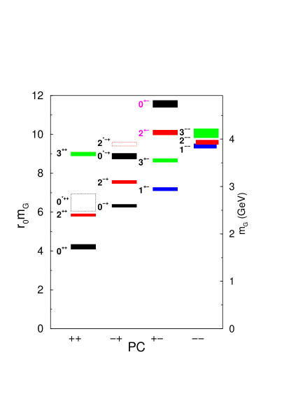
Figure 1: The mass of the glueball states. The scale is set by $r_{0}$ with $1/r_{0}=410(20)$ MeV. From Morningstar and Peardon [5].

3.1 Glueball Decays

We expect glueball decays to have flavour symmetric couplings to final state hadrons:

$${{\Gamma(G\to\pi\pi:\;K\bar{K}:\;\eta\eta:\;\eta\eta^{\prime}:\;\eta^{\prime}\eta^{\prime})}\over{\hbox{Phase Space}}}\simeq 3:4:1:0:1$$ (1)

The situation is complicated by mixing with $q\bar{q}$ and $q\bar{q}q\bar{q}$ so the physical states are linear combinations:

$$|f_{0}\rangle=\alpha|n\bar{n}\rangle+\beta|s\bar{s}\rangle+\gamma|G\rangle+\delta|q\bar{q}q\bar{q}\rangle$$ (2)

Mixing will both shift the unquenched glueball masses and distort the naive patterns of couplings given by eqn. (1) [6, 12].

Meson properties can be used to extract the mixings and understand the underlying dynamics. For example, central production of the isoscalar scalar mesons has found the ratio of partial widths $\Gamma(K\bar{K})/\Gamma(\pi\pi)$ to be [13]:

$$f_{0}(1370) <1 (0.5\pm 0.2)$$

$$f_{0}(1500) <<1 (0.3\pm 0.1)$$ (3)

$$f_{0}(1710) >>1 (5.5\pm 0.8)$$

Relating this information to theoretical expectations Close and Kirk find [12]:

$$|f_{0}(1370)\rangle = -0.79|n\bar{n}\rangle-0.13|s\bar{s}\rangle+0.60|G\rangle$$

$$|f_{0}(1500)\rangle = -0.62|n\bar{n}\rangle+0.37|s\bar{s}\rangle-0.69|G\rangle$$ (4)

$$|f_{0}(1710)\rangle = +0.14|n\bar{n}\rangle+0.9|s\bar{s}\rangle+0.39|G\rangle$$

A similar analysis was done by Amsler [14]. The point is not the details of a specific mixing calculation but that mixing is an important consideration that must be taken into account in the phenomenology.

Before proceeding to hadronic production of glueballs we mention that two photon couplings are a sensitive probe of $q\bar{q}$ content [12]. The L3 collaboration at LEP sees the $f_{0}(1380)$ and $f_{0}(1710)$ in $\gamma\gamma\to K\bar{K}$ but not the $f_{0}(1500)$. Because gluons do not carry electric charge, glueball production should be suppressed in $\gamma\gamma$ collisions. Quite some time ago Chanowitz [15] quantified this in a parameter he called “stickiness” given by the ratio of meson production in radiative $J/\psi$ decay to two photon couplings:

$$S={{\Gamma(J/\psi\to\gamma X)}\over{PS(J/\psi\to\gamma X)}}\times{{PS(\gamma\gamma\to X)}\over{\Gamma(\gamma\gamma\to X)}}$$ (5)

where $PS$ denotes phase space. A large value of $S$ is supposed to reflect an enhanced glue content.

3.2 Glueball Production

There are three processes which are touted as good places to look for glueballs:

1. $J/\psi\to\gamma X$

2. $p\bar{p}$ annihilation

3. $pp\to p_{f}(G)p_{s}$ central production

It is the latter process that is relevant to COMPASS. Central production is understood to proceed via gluonic pomeron exchange. It is expected that glueball production has to compete with $q\bar{q}$ production. However, a kinematic filter has been proposed which appears to suppress established $q\bar{q}$ states when in a P-wave or higher wave [16].

In the central production process:

$$pp\to p_{f}(G)p_{s}$$ (6)

$p_{s}$ and $p_{f}$ represent the slowest and fastest outgoing protons. Central production is believed to be dominated by double pomeron exchange. The pomeron is believed to have a large gluonic content. Folklore assumed that the pomeron has $J^{PC}=0^{++}$ quantum numbers and therefore gives rise to a flat distribution. But the distribution turns out not to be flat and is well modelled assuming a $J=1$ exchange particle [17]. In other words the pomeron transforms as a non-conserved vector current. Data from CERN experiment WA102 appears to support this hypothesis.

Close and Kirk [16] have found a kinematic filter that seems to suppress established $q\bar{q}$ states when they are in $P$ and higher waves. The pattern of resonances depends on the vector difference of the transverse momentum recoil of the final state protons:

$$dP_{T}=|\vec{k}_{T_{1}}-\vec{k}_{T_{2}}|$$ (7)

For $dP_{T}$ large, the well established $q\bar{q}$ states are prominent while for $dP_{T}$ small, the established $q\bar{q}$ states are suppressed and the $f_{0}(1500)$, $f_{0}(1710)$, and $f_{0}(980)$ survive.

Figure 2: The $\phi$ distributions for (a) $f_{0}(1370)$ (b) $f_{0}(1500)$ (c) $f_{2}(1270)$ (d) $f_{2}(1950)$ for the data (dots) and the Monte Carlo (histogram). From Close and Schuler [18].

Close, Kirk, and Schuler give a good account of the data by modeling the pomeron as a nonconserved vector exchange [18]. They find that the $\phi$ angular distribution, the angle between the $k_{T}$ vectors, appears to distinguish between the production of different states [17, 18]. In particular:

$0^{-+}$

Parity requires the vector pomeron to be transversely polarized. The distribution peaks at $90^{o}$.

$1^{++}$

One pomeron is transverse and the other longitudinal and the distribution peaks at $180^{o}$.

$2^{-+}$

Similar to the $0^{-+}$ case but peaks at $0^{o}$. Helicity 2 is suppressed by Bose statistics.

$2^{++}$

Established states peak at $180^{o}$ while the $f_{2}(1950)$ peaks at $0^{o}$.

$0^{-+}$

Some states peak at $0^{o}$ while others are spread out:

• $f_{0}(1500)$, $f_{0}(1710)$, and $f_{0}(980)$ peak at small $\phi$.

• $f_{0}(1370)$ peaks at large $\phi$.

The fact that the $f_{0}(1370)$ and $f_{0}(1500)$ have different $\phi$ dependence indicates that it is not just a $J$ dependent phenomena [19, 20].

The $0^{++}$ and $2^{++}$ expect both $TT$ and $LL$ contributions. The differential cross section is given by [18, 21]:

$${{d\sigma}\over{d\phi}}\sim\left[{1+{{\sqrt{t_{1}t_{2}}}\over{\mu^{2}}}{a_{t}\over a_{L}}\cos\phi}\right]^{2}$$ (8)

Differential cross sections for scalar and tensor mesons are shown in Fig. 2 [18, 21]. Good fits to the distributions are obtained by varying $\mu^{2}a_{L}/a_{T}$ with $\mu^{2}a_{L}/a_{T}$ $=-0.5$ GeV² for $f_{0}(1370)$, $=+0.7$ GeV² for $f_{0}(1500)$, $=-0.4$ GeV² for $f_{2}(1270)$, and $=+0.7$ GeV² for $f_{0}(1950)$. Thus, the $\phi$ distributions are fitted with only 1 parameter.

4 HYBRID MESONS

Hybrid mesons are defined as those in which the gluonic component is non-trivial. There are two types of hybrids; vibrational hybrids and topological hybrids. The hybrid spectrum is generated by generating effective potentials from adiabatically varying gluonic flux tubes. A given adiabatic surface corresponds to some string topology and excitation. This is illustrated in Fig. 3. In the flux-tube model the lowest excited adiabatic surface corresponds to transverse excitations of the flux tube.

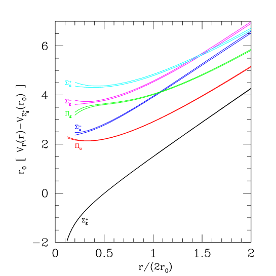
Figure 3: A set of hybrid adiabatic surfaces for static central potentials. $\Lambda=\Sigma,\;\Pi,\;\Delta,\ldots$ corresponds to the magnitude of $J_{glue}=0,\;1,\;2,\ldots$ projected onto the molecular axis. The superscript $=\pm$ corresponds to the even or oddness under reflections in a plane containing the molecular axis and the subscript $u/g$ corresponds to odd/even charge conjugation plus spatial inversion about the midpoint. The familiar $q\bar{q}$ potential is labelled as $\Sigma^{+}_{g}$ and the first-excited potential is the $\Pi_{u}$ so the lowest lying hybrid mesons should be based on this potential. The double lines on the excited surfaces indicate the calculational uncertainty in determining the potential. From Juge, Kuti and Morningstar [22].

While this picture is appropriate for heavy quarkonium it is not at all clear that it can be applied to light quark hybrids. Nevertheless, given that the constituent quark model works so well for light quarks, it is not unreasonable to also extend the flux tube description to light quarks. In the flux tube model the lowest mass hybrid mesons with light quark content have masses $\sim 1.9$ GeV [23, 24, 25]. There is a double degeneracy with $J^{PC}=0^{+-}$, $0^{-+}$, $1^{+-}$, $1^{-+}$, $2^{+-}$, $2^{-+}$, $1^{++}$, $1^{--}$ corresponding to the two transverse polarizations of the flux tube. The degeneracies are expected to be broken by the different excitation energies of the flux tube modes, spin dependent effects, and mixings with conventional $q\bar{q}$ states (and possibly $q\bar{q}q\bar{q}$). Lattice results are generally consistent with these predictions with $M(1^{-+})\sim 1.9$ GeV, $M(0^{+-})\sim 2.1$ GeV, and $M(2^{+-})\sim 2.1$ GeV [26, 27].

4.1 Hybrid Meson Decays

Decay properties are a crucial tool in both directing exotic hybrid meson searches and to distinguish hybrids with conventional quantum numbers from conventional $q\bar{q}$ states. A general selection rule for hybrid decays, which appears to be universal to all models, is that to preserve the symmetries of quark and colour fields about the quarks, the $\Pi_{u}$ hybrid must decay to a P-wave meson [28, 29]. In other words it cannot transfer angular momentum to relative angular momentum between final state mesons but rather, to internal angular momentum of one of the final state mesons. For the case of the $1^{-+}$ exotic the $\hat{\rho}\to b_{1}\pi,\;f_{1}\pi$ modes are expected to dominate.

To calculate hybrid properties we need to rely on models. We will use the results of the flux tube model [24, 30] which is based on strong coupling Hamiltonian lattice QCD. The degrees of freedom are quarks and flux-tubes. This model provides a unified framework for conventional hadrons, multiquark states, hybrids, and glueballs.

The flux-tube model predictions of Close and Page for the dominant decay widths of exotic hybrid mesons are given in Table 1 [30]. One can see that the $\hat{a}_{0}$ and $\hat{f}^{\prime}_{0}$ are too broad to be observed as resonances. The $\hat{\omega}_{1}$ decays to $a_{1}\pi$ and $K_{1}K$ as does the $\hat{\phi}_{1}$. These final states are notoriously difficult to reconstruct. Thus the best bets for finding exotic hybrids are the decays $\hat{\rho}_{1}\to[b_{1}\pi]_{S},\;[f_{1}\pi]_{S}$ with $\Gamma\simeq 170$ MeV. This is why the $\hat{\rho}$ is the focus of so much attention in hybrid searches. The narrow $f_{1}(1285)$ provides a particularly useful tag in $\hat{\rho}\to\pi f_{1}$. Although there is a general consensus among models with respect to the qualitative properties given here one should be aware that there is some disagreement in predictions. See, for example, the predictions of Page, Swanson and Szczepaniak [31, 32]. In particular, Page et al. [32] predict the $\hat{a}_{2}$ width to be very narrow so that it would be useful to search for $a_{2}\pi$ and $h_{1}\pi$ final states. If nothing else this would be a good test of the models.

Table 1: Dominant decay widths of exotic hybrid mesons. From Close and Page [30]. Initial State Final State L $\Gamma$ $\hat{\rho}(1^{-+})$ $b_{1}(1235)\pi$ S 100 D 30 $f_{1}(1285)\pi$ S 30 D 20 $\hat{\omega}(1^{-+})$ $a_{1}(1260)\pi$ S 100 D 70 $K_{1}(1400)K$ S 100 $\hat{\phi}(1^{-+})$ $K_{1}(1270)K$ D 80 $K_{1}(1400)K$ S 250 $\hat{a}_{2}(2^{+-})$ $a_{2}(1320)\pi$ P 450 $a_{1}(1260)\pi$ P 100 $h_{1}(1170)\pi$ P 150 $\hat{f}_{2}(2^{+-})$ $b_{1}(1235)\pi$ P 500 $\hat{f}_{2}^{\prime}(2^{+-})$ $K_{2}^{*}(1430)K$ P 250 $K_{1}(1400)K$ P 200 $\hat{a}_{0}(0^{+-})$ $a_{1}(1260)\pi$ P 800 $h_{1}(1170)\pi$ P 100 $\hat{f}_{0}(0^{+-})$ $b_{1}(1235)\pi$ P 250 $\hat{f}_{0}^{\prime}(0^{+-})$ $K_{1}(1270)K$ P 800 $K_{1}(1400)K$ P 50

Although hybrid mesons with exotic quantum numbers give a distinctive signature, hybrids with conventional quantum numbers are also expected in the meson spectrum. The situation is more complicated than simply looking for additional states because we expect strong mixing between non-spin exotic hybrids and conventional mesons with the same quantum numbers. Thus, to distinguish non-exotic hybrids from conventional states requires detailed predictions of properties [10, 30, 33, 34].

A first example is whether the $\pi(1800)$ is a conventional $3S$ isovector pseudoscalar meson (the 2nd radial excitation of the $\pi$) or a hybrid meson. Predictions for the partial width of a $\pi_{3S}$ and $\pi_{H}$ are given in Table 2. The flux tube model predicts that the $\pi_{3S}$ decays to $\omega\pi$ but the $\pi_{H}$ does not. Likewise, the $\pi_{H}$ has a large partial width to $f_{0}(1300)\pi$ while for the $\pi_{3S}$ this partial width is quite small. Therefore the $\rho\omega$ and $f_{0}(1300)\pi$ modes can be used as discrimators between the two possibilities. The $\pi_{3S}$ has been observed in $\pi f_{0}(1300)$ lending support to its identification as a hybrid.

Table 2: Partial decay widths for the $\pi(3S)$ and $\pi_{H}$. From Barnes it et al. [10]. State Partial widths to final states Total $\pi\rho$ $\omega\rho$ $\rho(1465)\pi$ $f_{0}(1300)\pi$ $f_{2}\pi$ $K^{*}K$ $\pi_{3S}(1800)$ 30 74 56 6 29 36 231 $\pi_{H}(1800)$ 30 — 30 170 6 5 $\sim 240$

Another example is that of the $\rho^{\prime}$ and $\omega^{\prime}$ mesons. One expects the physical vector mesons to be a linear combination

$$|V\rangle=\sum_{n}\alpha_{n}|n^{3}S_{1}\rangle+\sum_{m}\beta_{m}|m^{3}D_{1}\rangle+\gamma|V_{H}\rangle$$ (9)

To disentangle the various components of the physical mesons we need to perform a detailed comparison between the observed states and the predictions for the unmixed $q\bar{q}$ and $V_{h}$ states, much as was done for the scalar iso-scalar mesons. Partial width predictions are shown in Table 3 for the $\rho_{2S}(1465)$, $\rho_{1D}(1700)$, and $\rho_{H}(1500)$ states. For this example the $\pi h_{1}$ and $\pi a_{1}$ decay modes can discriminate between the $\rho_{2S}$, $\rho_{1D}$ and $\rho_{H}$ to disentangle the mixings.

Table 3: Partial decay widths for the $\rho_{2S}$, $\rho_{1D}$ and $\rho_{H}$. From Barnes it et al. [10]. State Partial widths to final states Total $\pi\pi$ $\omega\pi$ $\rho\eta$ $\rho\rho$ $KK$ $K^{*}K$ $h_{1}\pi$ $a_{1}\pi$ $\rho_{2S}(1465)$ 74 122 25 – 35 19 1 3 279 $\rho_{1D}(1700)$ 48 35 16 14 36 26 124 134 435 $\rho_{H}(1500)$ 0 5 1 0 0 0 0 140 $\sim 150$

A similar excercise can be applied to the isocalar sector with the relevant partial widths given in Table 4. The decays $\omega(1420)\to\pi b_{1}$ and $\omega(1600)\to\pi b_{1}$ are both observed to be small so neither is likely to be a pure $1^{3}D_{1}$ state. This implies that one is the $2^{3}S_{1}$ and indicates that the other has significant $\omega_{H}$ content. It is clearly important to find the 3rd state in this set and determine some of the other branching ratios. The essential point is that although the two states may have the same $J^{PC}$ quantum numbers they have different internal structure which will manifest itself in their decays. Unfortunately, nothing is simple and we once again point out that strong mixing is expected between hybrids with conventional quantum numbers and $q\bar{q}$ states with the same $J^{PC}$ so that the decay patterns of physical states may not closely resemble those of either pure hybrids or pure $q\bar{q}$ states. With enough information one could perform an analysis similar to the one performed on the scalar meson sector by Close and Kirk [12].

Table 4: Partial decay widths for the $\omega_{2S}$, $\omega_{1D}$ and $\omega_{H}$. From Barnes it et al. [10]. State Partial widths to final states Total $\rho\pi$ $\omega\eta$ $KK$ $K^{*}K$ $b_{1}\pi$ $\omega_{2S}(1419)$ 328 12 31 5 1 378 $\omega_{1D}(1649)$ 101 13 35 21 371 542 $\omega_{H}(1500)$ 20 1 0 0 0 $\sim 20$

4.2 Production of Hybrid Mesons

Hybrid mesons can be produced in a number of processes:

1. $J/\psi\to\gamma X$

2. $\bar{p}p$ annihilation

3. peripheral production

4. photoproduction

It is the latter two processes which are relevant to the COMPASS collaboration. Peripheral production is discussed in more detail by Dorofeev [35] and photoproduction by Moinester [36] in these proceedings.

4.2.1 Hadronic Peripheral Production

In peripheral production the beam particle is excited and exchanges momentum and quantum numbers with the target nucleus via an exchange particle. The excited meson continues to move forward, subsequently decaying into the decay products which are detected by the experiment. This is shown schematically in Fig. 4. Examples of experiments which studied peripheral production are LASS at SLAC, E852 at Brookhaven, BENKEI at KEK, VES at IHEP/Serpukhov and GAMS at CERN.

Figure 4: Peripheral production of mesons.

Evidence for hybrid mesons has been seen by the VES collaboration [37] in $\rho^{0}\pi^{-}$, $\pi\eta$, and $\pi b_{1}$ final states in the reaction

$$\pi^{-}N\to(\eta\pi^{+}\pi^{-})\pi^{-}N\hbox{ with a 37 GeV/c }\pi\hbox{ beam}$$ (10)

and by BNL E852 [38] in the final state $\pi f_{1}(1285)$ in the reaction

$$\pi^{-}p\to(\pi^{-}\pi^{+}\pi^{-})p\hbox{ with a 18 GeV/c }\pi\hbox{ beam.}$$ (11)

There is no reason a priori to expect that any type of hadron is preferred over any other in this mechanism. The $\pi$ exchange mechanism only provides access to natural parity states. But the advantage of very high statistics is that with enough statistics one could use $t$-distributions to distinguish between different exchange particles which would allow one to study states other than the natural parity states.

E852 at Brookhaven provides a nice lesson of the advantages of high statistics [38]. In Fig. 5 the event rates for $\pi^{-}p\to\pi^{+}\pi^{-}\pi^{-}p$ at 18 GeV/c is shown as a function of $\pi^{+}\pi^{-}\pi^{-}$ invariant mass. Structure is seen corresponding to the $a_{1}$, $a_{2}$, and $\pi_{2}$ mesons although it would be difficult to draw conclusions from this figure alone. However, with the large data sample a partial wave analysis can be performed. The results are also shown in Fig. 5. One now sees clear resonances corresponding to the $a_{1}$, $\pi_{2}$ and $a_{2}$. These reference waves can be used to measure the phase shift of the exotic waves that are being looked for. This is shown in Fig. 6 where intensity and phase of the $1^{-+}$ exotic signal clearly stands out.

The lesson is that a PWA is a necessary component of any study of meson physics and that high statistics offer the opportunity to perform the necessary studies.

       

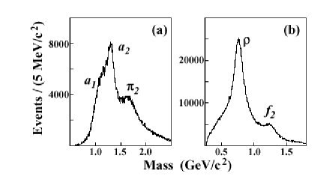
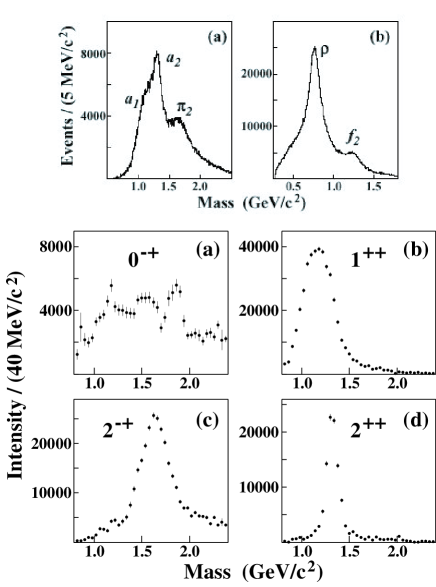
Figure 5: Invariant mass distribution of $\pi^{+}\pi^{-}\pi^{-}$. The figure on the left shows the raw data and the figure on the right shows the results of a PWA. From Ref. [38].

      

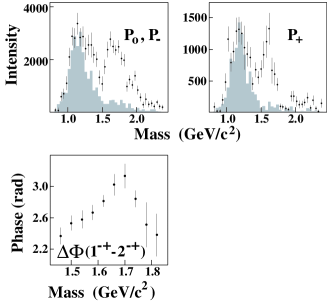
Figure 6: The figure on the left shows the wave intensities of the $1^{-+}$ exotic waves. The PWA fit to the data is shown as the points with error bars and the shaded histograms show estimated contributions from all nonexotic waves due to leakage. The figure on the right shows the phase difference between the $1^{-+}$ and $2^{-+}$ waves from a coupled mass-dependent Breit-Wigner fit. From Ref. [38].

4.2.2 Photoproduction

COMPASS offers a unique opportunity in that it can also study hybrid meson production via photoproduction by way of initial muon beams. Photoproduction is qualitatively different to hadronic peripheral production so that the series of preferred excitations is likely to be different. Additionally, it is a strong source of $s\bar{s}$ states. Via vector meson dominance one can view the photon as a linear combination of the $\rho$, $\omega$, $\phi$ and other vector mesons. In vector mesons the quark spins are aligned in a $S=1$ triplet state. As hybrid mesons with exotic quantum numbers are also in a spin triplet state it is believed that exotic hybrid mesons are favoured by this process. At the present time there is virtually no photoproduction data available. Some time ago the Omega Photon Collaboration studied the process $\gamma p\to(b_{1}\pi)p$ at 25-50 GeV incident energy witht the specific intention of seeking hybrids [39]. The most recent photoproduction experiment was done at SLAC studying $\gamma p\to\pi^{+}\pi^{+}\pi^{-}n$ at 19 GeV [40]. It showed hints of exotics but unfortunately, the statistics were rather low. A dedicated high statistics experiments with the power of modern detection and analysis should reexamine this process [41]. This is almost virgin territory and an area to which the COMPASS collaboration could make important contributions.

5 MULTIQUARK MESONS

In addition to conventional $q\bar{q}$ mesons, hybrids and glueballs, multiquark mesons are also expected to exist. It was noted in the discusions of glueballs and hybrids that they contribute to the physical spectrum.

While there is no room to discuss this topic in any detail I mention it as an additional ingredient that one should be aware of when studying meson spectroscopy. Several examples exist of multiquark candidates. It has long been believed that the $f_{0}(980)$ and $a_{0}(980)$ are multiquark states although their exact nature; a compact $q\bar{q}q\bar{q}$ object or an extended $K\bar{K}$ molecule is the focus of vigorous debate. The nature of the $f_{1}(1430)$ is a longstanding puzzle and is part of our lack of understanding of what is known as the $E/\iota$ puzzle. There is speculation that it is a $K^{*}K$ bound state.

Multiquark states can also have exotic quantum numbers. The best bets along this line of study would be fractional or doubly charged mesons although it has been speculated that at least one of the $J^{PC}=1^{-+}$ exotic candidates is a $\bar{q}q\bar{q}q$ object.

6 SUMMARY

The existence of non-$q\bar{q}$ mesons is the most important qualitative open question in QCD. The discovery and mapping out of the glueball and hybrid meson spectrum is a crucial test of QCD. It will help validate lattice QCD as an important computational tool for non-perturbative field theory. It will take detailed studies to distinguish glueball and hybrid candidates from conventional $q\bar{q}$ states. This will require extremely high statistics experiments to measure meson properties such as partial widths and production mechanisms. COMPASS is unique. It has numerous tools to do this via $\pi$, $K$, $p$, and $\mu$ beams. COMPASS can make important advances in this field. I strongly encourange you to do so.

References

- [1] For a recent review of meson spectroscopy see S. Godfrey and J. Napolitano, Rev. Mod. Phys. 71, 1411 (1999). See also F.E. Close, Int. J. Mod. Phys. A17, 3239 (2002). [hep-ph/0110081].
- [2] G.S. Bali, Phys. Rep. 343, 1 (2001) [hep-ph/0001312]; C. Davies, [hep-ph/0205181].
- [3] C. Michael, Proceedings of Wien 2000, Quark confinement and the hadron spectrum, p 197. [hep-ph/0009115].
- [4] Bali, G., K. Schilling, A. Hulsebos, A. Irving, C. Michael, and P. Stephenson, Phys. Lett. B309, 378 (1993); Morningstar, C. and Peardon, [hep-lat/9901004]; Lee, W., and D. Weingarten, [hep-lat/9805029]; Chen, K., J. Sexton, A. Vaccarino, and D. Weingarten, Nucl. Phys. B. (Proc. Suppl) 34, 357 (1994). Michael, C., 1998, Proceedings of the Seventh International Conference on Hadron Spectroscopy, ed. S.-U. Chung and H.J. Willutzki, Brookhaven National Laboratory New York, August 1997 (AIP Conference Proceedings 432, Woodbury New York) p. 657.
- [5] C. Morningstar and M. Peardon, Phys. Rev. D56, 4043 (1997); D60, 034509 (1999).
- [6] C. Amsler and F.E. Close, Phys. Rev. D53 ,295 (1996); Phys. Lett. B353, 385 (1995).
- [7] G.S. Bali, K. Schilling, and C. Schlichter, Phys. Rev. D51, 5165 (1995) [hep-lat/9409005].
- [8] K.J. Juge, J. Kuti, and C.J. Morningstar, Phys. Rev. Lett. 82, 4400 (1999); Nucl. Phys. B (Proc. Suppl.) 63A-C, 326 (1998).
- [9] A detailed account of conventional meson properties is given by: S. Godfrey and N. Isgur, Phys. Rev. D32, 189 (1985); Phys. Rev. D34, 899 (1986); S. Godfrey, Phys. Rev. D31, 2375 (1985); S. Godfrey, R. Kokoski, Phys. Rev. D43, 1679 (1991).
- [10] T. Barnes, F.E. Close, P.R. Page, and E.S. Swanson, Phys. Rev. D55, 4157 (1997).
- [11] T. Barnes, N. Black, and P.R. Page [nucl-th/0208072].
- [12] F. Close and Kirk, Phys. Lett. B483, 345 (2000); Eur. Phys. J. C21, 531 (2001).
- [13] B. Barberis et al, Phys. Lett. B479, 59 (2000).
- [14] C. Amsler, Phys. Lett. B541, 22 (2002).
- [15] Chanowitz, M., Proceedings of the VI International Workshop on Photon -Photon Collisions, Lake Tahoe, CA, Sept. 10-13, World Scientific, 1985, R.L. Lander, ed.
- [16] F. Close and Kirk, Phys. Lett. B397, 333 (1997).
- [17] B. Barberis et al, Phys. Lett. B467, 165 (1999).
- [18] F.E. Close and G.A. Schuler, Phys. Lett. B458, 127 (1999); B464, 279 (1999).
- [19] B. Barberis et al, Phys. Lett. B474, 423 (2000).
- [20] B. Barberis et al, Phys. Lett. B462, 462 (1999).
- [21] F. Close, Kirk, and Schuler, Phys. Lett. B477, 13 (2000).
- [22] K.J. Juge, J. Kuti, and C. Morningstar, Nucl. Phys. (Proc. Suppl.) 63A-C, 326 (1998).
- [23] N. Isgur and J. Paton, Phys. Rev. D31, 2910 (1985).
- [24] N. Isgur, R. Kokoski, and J. Paton, Phys. Rev. Lett. 54, 869 (1985).
- [25] T. Barnes, F.E. Close, and E.S. Swanson, Phys. Rev. D52, 5242 (1995).
- [26] C. Michael, [hep-ph/9911219].
- [27] P. Lacock, C. Michael, P. Boyle and P. Rowland, Phys. Rev. D54, 6997 (1996); Phys. Lett. B401, 308 (1997); C. Bernard et al., Phys. Rev. D56, 7039 (1997); Nucl. Phys. B (Proc. Suppl.) 73, 264 (1999); P. Lacock and K. Schilling, Nucl. Phys. B (Proc. Suppl.) 73, 261 (1999).
- [28] P. Page, Phys. Lett. B402, 183 (1997).
- [29] C. McNeile, C. Michael, and P. Pennanen, Phys. Rev. D65, 094505 (2002).
- [30] F. Close and P. Page, Nucl. Phys. B443, 233 (1995).
- [31] E. Swanson and A. Szczepaniak, Phys. Rev. D56, 5692 (1997).
- [32] P.R. Page, E. Swanson, and A. Szczepaniak, Phys. Rev. D59, 034016 (1999).
- [33] F. Close and P. Page, Phys. Rev. D56, 1584 (1997).
- [34] A. Donnachie and Yu.S. Kalashnikova, Phys.Rev. D60, 114011 (1999).
- [35] Dorofeev, these proceedings.
- [36] M. Moinester, these proceedings.
- [37] G.M. Beladidze, et al., (VES Collaboration) Phys. Lett. B313, 276 (1993).
- [38] Adams, G., et al., (E852 Collaboration) Phys. Rev. Lett. 81, 5760 (1998).
- [39] M. Atkinson et al., (Omega Photon Collaboration), Z. Phys. C34, 157 (1987).
- [40] G.T. Condo et al., Phys.Rev. D48, 3045 (1993).
- [41] F. Close and P. Page, Phys. Rev. D52, 1706 (1995).