1 Introduction

Compelling evidences in favor of neutrino oscillations, driven by small neutrino masses and neutrino mixing, were obtained in the Super-Kamiokande [1, 2, 3, 4, 5], SNO [6, 7, 8], KamLAND [9] and other atmospheric [10, 11], solar [12, 13, 14, 15] and long-baseline [16] neutrino experiments. These findings have brought the physics of massive and mixed neutrinos in the front line of the research in particle physics and astrophysics.

From all the existing terrestrial and astrophysical data it follows that neutrino masses are smaller than the masses of other fundamental fermions (lepton and quarks) by many orders of magnitude. There is a general consensus that the smallness of neutrino masses is due to New Physics beyond the Standard Model. In the most attractive see-saw mechanism of neutrino mass generation [18], the smallness of neutrino masses is due to the violation of the total lepton number on a scale which is much larger than the electroweak scale.

There are many open problems in the physics of massive and mixed neutrinos:

• How many light neutrinos with definite mass exist in nature?

  The minimal number of massive neutrinos is equal to the number of active (flavor) neutrinos (three). If, however, sterile neutrinos exist, the number of massive neutrinos is larger than three (see Refs. [19, 20]). The data of all the existing neutrino oscillation experiments (solar [12, 13, 14, 15, 5, 6, 7, 8], atmospheric [1, 2, 3, 10, 11] and LSND [21]) require the existence of (at least) four massive neutrinos. LSND is the single accelerator experiment in which the transition $\bar{\nu}_{\mu}\to\bar{\nu}_{e}$ has been observed. The check of the LSND claim is an urgent problem. This will be done by the MiniBooNE experiment [22], which started recently.

• What is the nature of the neutrinos with definite mass: are they purely neutral Majorana particles, or Dirac particles, possessing a conserved total lepton number?

  The answer to this fundamental question can be obtained through the investigation of processes in which the total lepton number is not conserved. The most promising process is neutrinoless double $\beta$-decay of some even-even nuclei. There are many new experiments on the search for neutrinoless double $\beta$-decay now in preparation (see Ref. [23]), which will push the experimental sensitivity at a level that is about two orders of magnitude better than today’s sensitivity. We will discuss neutrinoless double $\beta$-decay in this review.

• What are the absolute values of the neutrino masses?

  Neutrino oscillations are due to differences of phases which different massive components of the initial flavor neutrino states pick up during their evolution. As a result, neutrino oscillation experiments allow to obtain information only on neutrino mass-squared differences (see Refs. [24, 25, 19, 20]). It is very important that neutrino oscillation experiments are sensitive to tiny neutrino mass-squared differences, because of the possibility to explore very large distances and small energies. The measurement of the absolute values of neutrino masses at a level of a few eV is a challenging problem. This review is dedicated to the discussion of this problem (see also Ref. [26]).

Let us mention also the very important problems of the precise determination of the values of the neutrino oscillation parameters and the search for CP violation in neutrino oscillations. These problems will be investigated in experiments at the future Super-Beam facilities and Neutrino factories (see Refs. [27, 28, 29, 30]). We will not discuss them here.

We will start in Section 2 with a short review of the present status of neutrino oscillations. We will consider neutrino oscillations in solar, atmospheric and long-baseline neutrino experiments in the framework of mixing of three neutrinos. The importance for neutrino mixing of the results of the long-baseline reactor experiments CHOOZ and Palo Verde, in which no indication in favor of neutrino oscillations was found, will be stressed.

In Section 3 we will consider the Mainz [31, 32, 33] and Troitsk [34, 35] experiments on the measurement of the neutrino mass through the detailed investigation of the end-point part of the $\beta$-spectrum of tritium. We will discuss also the future KATRIN tritium experiment [36].

In Section 4 we briefly review the most recent results of the experiments on the measurement of the effect of neutrino masses in pion and tau decays.

Section 5 is dedicated to neutrinoless double $\beta$-decay. Even though in this review we are mainly interested in the possibilities to obtain information about the absolute values of the neutrino masses from the investigation of this process, some aspects of the theory of the process will be also presented.

The role of neutrinos in Astrophysics and Cosmology has been under the scrutiny of physicists with ever increasing intensity over the last few decades (see Refs. [26, 37, 38, 39, 40, 41, 42, 43, 44]). Actually, the intimate relationship of neutrinos and astrophysics goes even further back in time when Bethe and others realized that the inner workings of the Sun proceed via the thermonuclear reactions that burn hydrogen into helium and release neutrinos. Since then there has been a steady increase in interest and involvement in the study of neutrinos in astrophysical environments. Not only the interest in solar neutrinos has been particularly intense over the last years, where such epochal events as their detection on Earth in a variety of underground experiments have been milestones of late 20th century high energy physics, but also the involvement of neutrinos in stellar core collapse has been theoretically analyzed and observationally established in the momentous detection of neutrinos of SN1987A and, furthermore, the influence and role of neutrinos in the cosmic evolution has been a major area of research in contemporary high energy physics.

Seminal work on neutrinos and Cosmology was pursued in the late sixties and early seventies when neutrinos appeared as ideal candidates to contribute substantially to the matter density of the Universe (see Ref. [45]). In fact, hot dark matter models were popular for quite some time as they seemed to render a satisfactory model for structure formation. Of course, the interest in neutrinos worked then and still works now both ways; from the cosmological arena, neutrinos were welcomed in the new cosmological Paradigm but also from the Particle Physics side, Cosmology/Astrophysics was used and is used even more so today to constrain and sharpen the still not well known properties of neutrinos.

The main focus of this review is the mass of neutrinos and especially their absolute mass. So we have selected the issues in Cosmology/Astrophysics that have relevant impact on the extraction of information concerning neutrino mass. They are contained in Sections 6, 7 and 8. We start in Subsection 6.1 by introducing the famous Gerstein-Zeldovich upper bound on the total sum of neutrino masses that can contribute to the matter density of the Universe [46, 47]. Subsection 6.2 is dedicated to an overview of the temperature fluctuations of the Cosmic Microwave Background Radiation (CMB) with a special attention to the characteristics of the peak structure of the angular power spectrum (see Ref. [48]). There, the influence of neutrino mass on the anisotropy spectrum is explicitly discussed. Although it is shown that this influence is not as significant as the role of other cosmological parameters that enter the angular spectrum of temperature fluctuations, Subsection 6.2 is relatively long as compared to the other Subsections in Section 6 because in any analysis of cosmological import the CMB is of pivotal importance. Subsection 6.3 is devoted to Galaxy Redshift Surveys. Neutrino mass has a remarkable effect on the power spectrum of matter distribution and this effect is observable in the large samples of data compiled in present galaxy distribution surveys or to be collected in future surveys. The final astrophysical source of information discussed in this review, namely Lyman $\alpha$ forests studies, is dealt with in Subsection 6.4. The last Subsection in Section 6, Subsection 6.5, contains the summary of all relevant neutrino mass limits obtained in the actual analysis by different groups and by different authors of the astrophysical/cosmological sources that have been discussed in the foregoing Subsections. It contains also a brief report on the prospects for neutrino mass in this rapidly changing field of Cosmology and Astrophysics.

Another topic that we cover in our review concerns cosmic rays. A probe of neutrino properties could come from the observation of cosmic rays with energies exceeding the Greisen-Zapsepin-Kuzmin cutoff [49, 50]. A possible explanation could be the so-called $Z$-burst scenario [51, 52], where a flux of ultra high energy neutrinos interacts with relic cosmological neutrinos, producing cosmic rays through the $Z$-resonance. The resonance condition involves the masses of neutrinos and we review the status of this mechanism in Section 7 (see also Ref. [26]).

In 1987 the observation of neutrinos coming from supernova 1987A in the Large Magellanic Cloud marked the beginning of extra solar system neutrino astronomy and allowed to get information on the supernova mechanism and neutrino properties (see Refs. [53, 54]). In particular, the values of the neutrino masses are limited by the lack of spread of the observed neutrino signal, which would be caused by energy-dependent velocities of sufficiently massive neutrinos [55, 56, 57, 58, 59]. In Section 8 we review the classification and rate of supernovae (Section 8.1), the current theory of core-collapse supernova dynamics (Section 8.2), the observation of SN1987A neutrinos (Section 8.3), the inferred limits on neutrino masses (Section 8.4), and the future prospects for supernova neutrino detection (Section 8.5).

2 Status of neutrino oscillations

Strong evidences in favor of neutrino oscillations were obtained recently in Super-Kamiokande [1, 2, 3, 4, 5], SNO [6, 7, 8], KamLAND [9] and other atmospheric [10, 11], solar [12, 13, 14, 15] and long-baseline [16] neutrino experiments. These findings gave us the first evidence that neutrino masses are different from zero and the fields of neutrinos with definite mass $\nu_{i}$ enter into the standard charged current (CC) and neutral current (NC)

$$j^{\mathrm{CC}}_{\alpha}=\sum_{l=e,\mu,\tau}\bar{\nu}_{lL}\gamma_{\alpha}l_{L}\,,\qquad j^{\mathrm{NC}}_{\alpha}=\sum_{l=e,\mu,\tau}\bar{\nu}_{lL}\gamma_{\alpha}\nu_{lL}$$ (2.1)

in the mixed form

$$\nu_{lL}=\sum_{i}U_{li}\nu_{iL}\qquad(l=e,\mu,\tau)\,,$$ (2.2)

where $U$ is the unitary mixing matrix. The minimal number of massive neutrinos $\nu_{i}$ is equal to the number of active (flavor) neutrinos (three). The number of massive neutrinos can be larger than three (see Ref. [19]). In this case, in addition to Eq. (2.2) we have

$$\nu_{sL}=\sum_{i}U_{si}\nu_{iL}\,,$$ (2.3)

where $\nu_{sL}$ ($s=s_{1},s_{2},\ldots$) are the fields of sterile neutrinos.

The most plausible mechanism of neutrino mass generation is the see-saw mechanism [18]. In order to explain this mechanism, let us consider the simplest case of one generation and assume that the standard Higgs mechanism with one Higgs doublet generates the Dirac mass term

$$\mathcal{L}^{\mathrm{D}}=-m_{\mathrm{D}}\,\bar{\nu}_{R}\nu_{L}+\mathrm{h.c.}\,.$$ (2.4)

It is natural to expect that $m_{\mathrm{D}}$ is of the same order of magnitude as the mass of the charged lepton or quarks in the same generation. We know, however, from experimental data that neutrino masses are much smaller than the masses of charged leptons and quarks. In order to “suppress” the neutrino mass let us assume that there is a lepton-number violating mechanism beyond the Standard Model which generates the right-handed Majorana mass term

$$\mathcal{L}^{\mathrm{Mj}}_{R}=-\frac{1}{2}\,M_{R}\,\bar{\nu}_{R}\,(\nu_{R})^{c}+\mathrm{h.c.}\,,$$ (2.5)

with $M_{R}\gg m_{\mathrm{D}}$ (usually it is assumed that $M_{R}\simeq M_{\mathrm{GUT}}\sim 10^{15}\,\mathrm{GeV}$). Here $(\nu_{R})^{c}=\mathcal{C}\overline{\nu_{R}}^{T}$, where $\mathcal{C}$ is the charge conjugation matrix.

After the diagonalization of the total neutrino mass term, for the light neutrino mass we obtain

$$m=-\frac{1}{2}\,M_{R}+\frac{1}{2}\,\sqrt{M_{R}^{2}+4\,m_{\mathrm{D}}^{2}}\simeq\frac{m_{\mathrm{D}}^{2}}{M_{R}}\ll m_{\mathrm{D}}$$ (2.6)

In the case of three generations, the see-saw mechanism leads to a spectrum of masses of Majorana particles with three light neutrinos with masses $m_{i}$ ($i=1,2,3$) much smaller than the quark and charged-lepton masses, and three very heavy masses of the order of the scale of violation of the total lepton number (for recent reviews see [60, 61]).

Let us stress that, if the neutrino masses have a standard see-saw origin, neutrinos with definite masses are Majorana particles. In some models which implement the see-saw mechanism (see, for example, Ref. [61]), the neutrino masses naturally satisfy the hierarchy

$$m_{1}\ll m_{2}\ll m_{3}\,.$$ (2.7)

If there is neutrino mixing, the state of a neutrino (active or sterile) with momentum $\vec{p}$ is given by the coherent superposition of the states of neutrinos with definite masses

$$|\nu_{\alpha}\rangle=\sum_{i}U_{\alpha i}^{*}\,|\nu_{i}\rangle\,,$$ (2.8)

where $|\nu_{i}\rangle$ is the state of neutrinos with momentum $\vec{p}$, mass $m_{i}$ and energy

$$E_{i}=\sqrt{p^{2}+m_{i}^{2}}\simeq p+\frac{m_{i}^{2}}{2p}\qquad(p^{2}\gg m_{i}^{2})\,.$$ (2.9)

From Eq. (2.8) it follows that if at time $t=0$ a neutrino $\nu_{\alpha}$ ($\alpha=e,\mu,\tau$) is produced, the probability amplitude to find $\nu_{\alpha^{\prime}}$ at time $t$ is given by

$$A(\nu_{\alpha}\to\nu_{\alpha^{\prime}})=\langle\nu_{\alpha^{\prime}}\,|e^{-iH_{0}\,t}\,|\nu_{\alpha}\rangle=\sum_{i}U_{\alpha^{\prime}i}\,e^{-iE_{i}t}\,U_{\alpha i}^{*}\,.$$ (2.10)

Thus, the probability of the transition $\nu_{\alpha}\to\nu_{\alpha^{\prime}}$ in vacuum is given by

$$\mathrm{P}(\nu_{\alpha}\to\nu_{\alpha^{\prime}})=\left|\delta_{{\alpha^{\prime}}\alpha}+\sum_{i\geq 2}U_{\alpha^{\prime}i}U_{\alpha i}^{*}\left(e^{-i\Delta{m}^{2}_{i1}\frac{L}{2E}}-1\right)\right|^{2}\,.$$ (2.11)

Here $\Delta{m}^{2}_{i1}=m^{2}_{i}-m^{2}_{1}$, $L\simeq t$ is the distance between the neutrino source and the neutrino detector, and $E$ is the neutrino energy.

In the simplest case of transitions between two types of neutrinos ($\nu_{\mu}\to\nu_{\tau}$ or $\nu_{\mu}\to\nu_{e}$, etc.), the index $i$ in Eq. (2.11) takes only one value $i=2$ and for the transition probability we obtain the standard expression

$$\mathrm{P}(\nu_{\alpha}\to\nu_{\alpha^{\prime}})=\frac{1}{2}\,\sin^{2}2\vartheta\left(1-\cos\Delta{m}^{2}\frac{L}{2E}\right)\qquad(\alpha^{\prime}\neq\alpha)\,,$$ (2.12)

where $\Delta{m}^{2}=m^{2}_{2}-m^{2}_{1}$, $|U_{\alpha 2}|^{2}=\cos^{2}\vartheta$, $|U_{\alpha^{\prime}2}|^{2}=1-|U_{\alpha 2}|^{2}=\sin^{2}\vartheta$ ($\vartheta$ is the mixing angle). For the probability of $\nu_{\alpha}$ to survive we have

$$\mathrm{P}(\nu_{\alpha}\to\nu_{\alpha})=1-\mathrm{P}(\nu_{\alpha}\to\nu_{\alpha^{\prime}})=1-\frac{1}{2}\,\sin^{2}2\vartheta\left(1-\cos\Delta{m}^{2}\frac{L}{2E}\right)\,.$$ (2.13)

The expressions (2.12) and (2.13) describe periodical transitions between two types of neutrinos (neutrino oscillations). They are widely used in the analysis of experimental data.

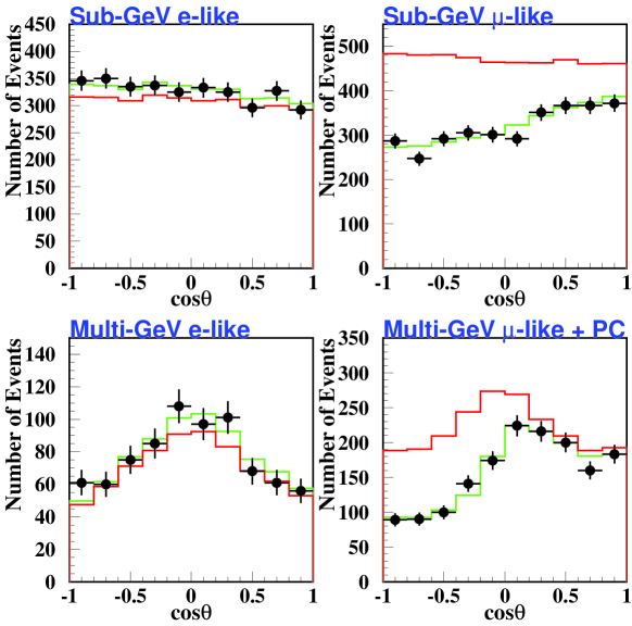
Figure 1: Zenith angle distribution of Super-Kamiokande sub-GeV single ring $e$-like events, $\mu$-like events, multi-GeV single ring $e$-like events, and $\mu$-like events + partially contained (PC) events. The black histogram shows the Monte Carlo prediction and the gray histogram is the best fit for $\nu_{\mu}\to\nu_{\tau}$ oscillations with $\Delta m^{2}=2.5\times 10^{-3}\,\mathrm{eV}^{2}$ and $\sin^{2}2\vartheta=1.0$. Figure taken from Ref. [64].

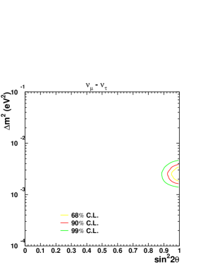
Figure 2: Allowed region of the oscillation parameters $\mathsf{\Delta{m}^{2}}=\Delta{m}^{2}_{\mathrm{atm}}$ and $\mathsf{\sin^{2}2\theta}=\sin^{2}2\vartheta_{\mathrm{atm}}$ from the analysis of Super-Kamiokande atmospheric neutrino data. Figure taken from Ref. [65].

2.1 Atmospheric neutrinos

The first model independent evidence in favor of neutrino oscillations was obtained in the atmospheric Super-Kamiokande (S-K) experiment [1, 2, 3]. In this experiment a significant zenith angle $\theta_{z}$ asymmetry of the high energy muon events was observed. At high energies the zenith angle $\theta_{z}$ is determined by the distance $L$, which neutrinos pass from the production region in the atmosphere to the detector. If there are no neutrino oscillations, the number of detected multi-GeV ($E\geq 1.3$ GeV) electron (muon) events satisfy the symmetry relation

$$N_{l}(\cos\theta_{z})=N_{l}(-\cos\theta_{z})\qquad(l=e,\mu)$$ (2.14)

As one can see from Fig. 1, the number of multi-GeV electron events observed in the S-K experiment is in good agreement with this relation. On the other hand, Fig. 1 shows that the multi-GeV muon events observed in the S-K experiment strongly violate the relation (2.14). Let us define the ratio $U/D$, where $U$ is the number of up-going muons ($-1\leq\cos\theta_{z}\leq-0.2$, $500\,\mathrm{km}\lesssim L\lesssim 13000\,\mathrm{km}$) and $D$ is the number of down-going muons ($0.2\leq\cos\theta_{z}\leq 1$, $20\,\mathrm{km}\lesssim L\lesssim 500\,\mathrm{km}$). For the multi-GeV events in the S-K experiment it was found [66]

$$\frac{(U/D)_{\mathrm{meas}}}{(U/D)_{\mathrm{MC}}}=0.54\pm 0.04\,\mbox{(stat.)}\pm 0.01\,\mbox{(syst.)}\,,$$ (2.15)

where $(U/D)_{\mathrm{MC}}$ is the ratio predicted by Monte Carlo under the assumption that there are no neutrino oscillations. If there are no neutrino oscillations, the ratio of ratios ${(U/D)_{meas}}/{(U/D)_{\mathrm{MC}}}$ must be equal to one. The S-K value (2.15) differs from one by $11\,\sigma$.

The data of the S-K [1, 2, 3] and other atmospheric neutrino experiments (SOUDAN 2 [10], MACRO [11]) are well described assuming that two-neutrino oscillations $\nu_{\mu}\to\nu_{\tau}$ take place. The allowed region of the neutrino oscillation parameters $\Delta{m}^{2}_{\mathrm{atm}}$ and $\sin^{2}2\vartheta_{\mathrm{atm}}$ from the analysis of the S-K data is shown in Fig. 2. At 90% $\mathrm{C.L.}$ the oscillation parameters are in the ranges

$$1.6\times 10^{-3}\leq\Delta{m}^{2}_{\mathrm{atm}}\leq 3.9\times 10^{-3}\,\mathrm{eV}^{2}\,,\qquad\sin^{2}2\vartheta_{\mathrm{atm}}>0.92\,.$$ (2.16)

The best-fit values of the parameters are

$$\Delta{m}^{2}_{\mathrm{atm}}=2.5\times 10^{-3}\mathrm{eV}^{2}\,,\qquad\sin^{2}2\vartheta_{\mathrm{atm}}=1.0\qquad(\chi^{2}_{\mathrm{min}}=163.2/170\,\mathrm{d.o.f.})\,.$$ (2.17)

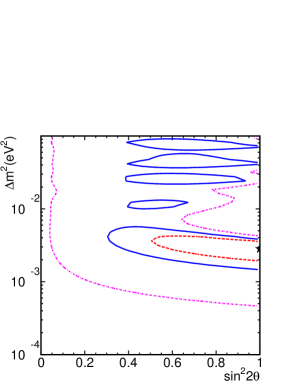
Figure 3: Allowed regions of the oscillation parameters $\mathsf{\Delta{m}^{2}}=\Delta{m}^{2}_{\mathrm{K2K}}$ and $\mathsf{\sin^{2}2\theta}=\sin^{2}2\vartheta_{\mathrm{K2K}}$ obtained from the results of the K2K experiment. The dashed, solid and dot-dashed lines are, respectively, 68.4%, 90% and 99% C.L. contours. The best fit point is indicated by the star. Figure taken from Ref. [16].

Recently the results of the first long-baseline accelerator experiment K2K have been published [16]. In this experiment neutrino oscillations in the atmospheric range of $\Delta{m}^{2}$ were searched for. Neutrinos mainly from decays of pions, produced by 12 GeV protons hitting a beam-dump target at the KEK proton accelerator, were detected by the S-K detector at the distance of about 250 km from the source. The average neutrino energy is 1.3 GeV.

In the K2K experiment there are two near detectors at the distance of about 300 m from the beam-dump target: a 1 kt water Cherenkov detector and a fine-grained detector. The number and the spectrum of muon neutrinos detected in S-K are compared with the expected quantities, calculated on the basis of the results of the near detectors. Quasielastic one-ring events $\nu_{\mu}+n\to\mu^{-}+p$ are selected for the measurement of the energy of the neutrinos.

The total number of muon events observed in the S-K experiment is 56. The expected number of events is $80.1^{+6.2}_{-5.4}$. The observed number of one-ring muon events that was used for the calculation of the neutrino spectrum is 29. The expected number of one-ring events is 44.

The regions of the allowed values of the oscillation parameters obtained from a maximum likelihood two-neutrino oscillation analysis of the K2K data are presented in Fig. 3. The best-fit values of the parameters are

$$\sin^{2}2\vartheta_{\mathrm{K2K}}=1\,,\qquad\Delta{m}^{2}_{\mathrm{K2K}}=2.8\times 10^{-3}\,\mathrm{eV}^{2}\,.$$ (2.18)

These values are in agreement with the values of the oscillation parameters obtained from the analysis of the S-K atmospheric neutrino data (see Eqs. (2.16) and (2.17)).

Thus, the K2K experiment confirms the evidence for neutrino oscillations that was found in the atmospheric Super-Kamiokande experiment. The K2K data reported in Ref. [16] have been obtained with $4.8\times 10^{19}$ protons on target (POT). The K2K experiment is planned to continue until about $10^{20}$ POT will be reached.

2.2 Solar neutrinos

The event rates measured in all solar neutrino experiments are significantly smaller than the event rates predicted by the Standard Solar models. The following values were obtained, respectively, for the ratio of the rates observed in the Homestake [12], GALLEX-GNO [13, 14], SAGE [67] and S-K [5, 68] experiments and those predicted by the BP00 [69] Standard Solar Model (SSM): $0.34\pm 0.03$, $0.58\pm 0.05$, $0.60\pm 0.05$, $0.465\pm 0.018$. It has been known during many years that these data can be explained by transitions of the initial solar $\nu_{e}$’s into other neutrinos, which cannot be detected in the radiochemical Homestake, SAGE, GALLEX and GNO experiments. The S-K experiment is sensitive mainly to $\nu_{e}$’s.

Recently, strong model independent evidence in favor of the transitions of solar $\nu_{e}$’s into $\nu_{\mu}$’s and $\nu_{\tau}$’s has been obtained in the SNO experiment [6, 7, 8]. In this experiment solar neutrinos are detected via the observation of the following three reactions:

• The charged-current (CC) reaction

  $$\nu_{e}+d\to e^{-}+p+p\,,$$ (2.19)

• The neutral-current (NC) reaction

  $$\nu_{x}+d\to\nu_{x}+n+p\,,$$ (2.20)

• The elastic-scattering (ES) reaction

  $$\nu_{x}+e\to\nu_{x}+e\,.$$ (2.21)

The kinetic energy threshold for the detection of electrons in the CC and ES processes in the SNO experiment is 5 MeV. The NC process has been detected through the observation of $\gamma$ rays from the capture of neutrons by deuterium. The NC threshold is 2.2 MeV. Thus, practically only neutrinos from ${}^{8}\mathrm{B}$ decay are detected in the experiment.

The measurement of the total CC event rate allows to determine the flux of $\nu_{e}$ on the Earth,

$$\Phi_{\nu_{e}}^{\mathrm{CC}}=\langle P(\nu_{e}\to\nu_{e})\rangle_{\mathrm{CC}}\,\Phi_{\nu_{e}}^{0}\,,$$ (2.22)

where $\Phi_{\nu_{e}}^{0}$ is the total initial flux of $\nu_{e}$’s and $\langle P(\nu_{e}\to\nu_{e})\rangle_{\mathrm{CC}}$ is the probability of $\nu_{e}$ to survive averaged over the CC cross section and the known initial spectrum of ${}^{8}\mathrm{B}$ neutrinos. In the SNO experiment it was found that

$$(\Phi_{\nu_{e}}^{\mathrm{CC}})_{\mathrm{SNO}}=\left(1.76{}^{+0.06}_{-0.05}\mbox{(stat.)}{}^{+0.09}_{-0.09}\mbox{(syst.)}\right)\times 10^{6}\,\mathrm{cm}^{-2}\,\mathrm{s}^{-1}\,.$$ (2.23)

All active neutrinos $\nu_{e}$, $\nu_{\mu}$ and $\nu_{\tau}$ are recorded by the detection of the NC process (2.20). Taking into account the universality of neutral currents (see the recent analysis in Ref. [70]), the total flux of all active neutrinos on the Earth measured in the SNO experiment is

$$(\Phi_{\nu}^{\mathrm{NC}})_{\mathrm{SNO}}=\sum_{l=e,\mu,\tau}(\Phi_{\nu_{l}}^{\mathrm{NC}})_{\mathrm{SNO}}=\left(5.09{}^{+0.44}_{-0.43}\mbox{(stat.)}{}^{+0.46}_{-0.43}\mbox{(syst.)}\right)\times 10^{6}\,\mathrm{cm}^{-2}\,\mathrm{s}^{-1}\,,$$ (2.24)

which is about three times larger than the CC flux in Eq. (2.23).

All active neutrinos are detected also via the observation of the ES process (2.21). However, the cross section of the neutral-current $\nu_{\mu,\tau}e\to\nu_{\mu,\tau}e$ scattering is about six times smaller than the cross section of the charged-current and neutral-current $\nu_{e}e\to\nu_{e}e$ scattering.

The event rate $R^{\mathrm{ES}}$ of the ES process (2.21) can be written as

$$R^{\mathrm{ES}}=\langle\sigma_{\nu_{e}e}\rangle\,\Phi_{\nu}^{\mathrm{ES}}\,.$$ (2.25)

Here $\langle\sigma_{\nu_{e}e}\rangle$ is the $\nu_{e}e\to\nu_{e}e$ cross section averaged over the initial spectrum of ${}^{8}\mathrm{B}$ neutrinos and the ES flux $\Phi_{\nu}^{\mathrm{ES}}$ is given by

$$\Phi_{\nu}^{\mathrm{ES}}=\Phi_{\nu_{e}}^{\mathrm{ES}}+\frac{\langle\sigma_{\nu_{\mu}e}\rangle}{\langle\sigma_{\nu_{e}e}\rangle}\,\Phi_{\nu_{\mu,\tau}}^{\mathrm{ES}}\,,$$ (2.26)

where $\Phi_{\nu_{e}}$ and $\Phi_{\nu_{\mu,\tau}}$ are, respectively, the fluxes of $\nu_{e}$ and $\nu_{\mu,\tau}$ on the Earth averaged over the ES cross section and the initial spectrum of ${}^{8}\mathrm{B}$ neutrinos. The ratio of the averaged $\nu_{\mu,\tau}e\to\nu_{\mu,\tau}e$ and $\nu_{e}e\to\nu_{e}e$ cross sections is given by

$$\frac{\langle\sigma_{\nu_{\mu}e}\rangle}{\langle\sigma_{\nu_{e}e}\rangle}\simeq 0.154\,.$$ (2.27)

In the SNO experiment [8] it was found

$$(\Phi_{\nu}^{\mathrm{ES}})_{\mathrm{SNO}}=\left(2.39{}^{+0.24}_{-0.23}\mbox{(stat.)}\pm 0.12\mbox{(syst.)}\right)\times 10^{6}\,\mathrm{cm}^{-2}\,\mathrm{s}^{-1}\,.$$ (2.28)

This value is in good agreement with the value of the ES flux determined in the S-K experiment [5, 68]. In the S-K experiment solar neutrinos are detected via the observation of the ES process (2.21). During 1496 days of running a large number, $22400\pm 800$, of solar neutrino events with recoil energy above the 5 MeV threshold were recorded (the uncertainty is due to the statistical subtraction of background events). From the data of the S-K experiment it was obtained

$$(\Phi_{\nu}^{\mathrm{ES}})_{\mathrm{S-K}}=\left(2.35\pm 0.02\mbox{(stat.)}\pm 0.08\mbox{(syst.)}\right)\times 10^{6}\,\mathrm{cm}^{-2}\,\mathrm{s}^{-1}\,.$$ (2.29)

In the S-K experiment also the spectrum of the recoil electrons was measured. No significant distortion of the spectrum with respect to the expected one (calculated under the assumption that the shape of the spectrum of $\nu_{e}$ on the Earth is given by the known initial ${}^{8}\mathrm{B}$ spectrum) was observed. Furthermore, no distortion of the spectrum of the electrons produced in the CC process (2.19) was observed in the SNO experiment. These data are compatible with the assumption that the probability of solar neutrinos to survive is a constant in the high energy ${}^{8}\mathrm{B}$ region. Thus, we have

$$\Phi_{\nu_{e}}^{\mathrm{NC}}\simeq\Phi_{\nu_{e}}^{\mathrm{CC}}\simeq\Phi_{\nu_{e}}^{\mathrm{ES}}\,.$$ (2.30)

Obviously, the NC flux can be presented in the form

$$\Phi_{\nu}^{\mathrm{NC}}=\Phi_{\nu_{e}}^{\mathrm{NC}}+\Phi_{\nu_{\mu,\tau}}^{\mathrm{NC}}\,.$$ (2.31)

Combining the CC and NC fluxes and using the relation (2.31), we can determine now the flux $\Phi_{\nu_{\mu,\tau}}^{\mathrm{NC}}$. In Ref. [7] the ES flux (2.28) was also taken into account as an additional constraint (see Fig. 4). The resulting flux of $\nu_{\mu}$ and $\nu_{\tau}$ on the Earth is

$$(\Phi_{\nu_{\mu,\tau}})_{\mathrm{SNO}}=\left(3.41{}^{+0.45}_{-0.45}\mbox{(stat.)}{}^{+0.48}_{-0.45}\mbox{(syst.)}\right)\times 10^{6}\,\mathrm{cm}^{-2}\,\mathrm{s}^{-1}\,.$$ (2.32)

Thus, the detection of the solar neutrinos through the simultaneous observation of CC, NC and ES processes allowed the SNO collaboration to obtain a direct model independent $5.3\,\sigma$ evidence of the presence of $\nu_{\mu}$ and $\nu_{\tau}$ in the flux of the solar neutrinos on the Earth.

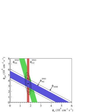
Figure 4: Flux of $\nu_{\mu}$ and $\nu_{\tau}$ vs flux of $\nu_{e}$ in the ⁸B energy range deduced from the three neutrino reactions in SNO. The diagonal bands show the total ⁸B flux as predicted by the BP00 SSM [69] (dashed lines) and that measured with the NC reaction in SNO (solid band). The intercepts of these bands with the axes represent the $\pm 1\sigma$ errors. The bands intersect at the fit values for $\phi_{e}\equiv\Phi_{\nu_{e}}$ and $\phi_{\mu\tau}\equiv\Phi_{\nu_{\mu,\tau}}$, indicating that the combined flux results are consistent with neutrino flavor transformation assuming no distortion in the ⁸B neutrino energy spectrum. Figure taken from Ref. [7].

Before the publication of the first results [6] of the SNO experiment, from the global fit of the data of the Homestake [12], SAGE [15], GALLEX [13], GNO [14] and S-K [71, 72] experiments several allowed regions in the plane of the two-neutrino oscillation parameters $\Delta{m}^{2}_{\mathrm{sol}}$ and $\tan^{2}\vartheta_{\mathrm{sol}}$ had been found: the large mixing angle (LMA), low mass (LOW) and small mixing angle (SMA) Mikheev-Smirnov-Wolfenstein (MSW) [73, 74] regions, the vacuum oscillation (VAC) region and others (see, for example, Ref. [19, 75]). The situation changed after the publication of the first SNO data [6], which, together with the recoil electron spectrum measured in the S-K experiment [71, 72, 4], disfavored the SMA-MSW region (see, for example, Ref. [76]). The most recent data from the SNO [7, 8] and S-K [5, 68] experiments strongly disfavor the SMA-MSW region (see, for example, Ref. [77]). All global analyses of the present solar neutrino data favor the LMA-MSW region [8, 78, 77, 79, 5, 80, 81, 82, 83]. The best-fit values of the oscillation parameters in the LMA-MSW region found in Ref. [8] are

$$\Delta{m}^{2}_{\mathrm{sol}}=5\times 10^{-5}\,\mathrm{eV}^{2}\,,\qquad\tan^{2}\vartheta_{\mathrm{sol}}=3.4\times 10^{-1}\,,\qquad(\chi^{2}_{\mathrm{min}}=57.0\,,\,72\,\mbox{d.o.f.})$$ (2.33)

In the next Subsection we will discuss the recent results of the long-baseline reactor experiment KamLAND [9]. The data of this experiment allow to exclude the SMA, LOW and VAC regions, leaving the LMA region as the only viable solution of the solar neutrino problem.

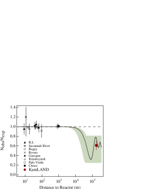
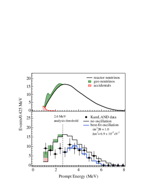
Figure 5: Left: The ratio of measured to expected $\bar{\nu}_{e}$ flux from reactor experiments. The shaded region indicates the range of flux predictions corresponding to the 95% C.L. LMA region found in a global analysis of the solar neutrino data [82]. The dotted curve corresponds to the best-fit values $\Delta{m}^{2}_{\mathrm{sol}}=5.5\times 10^{-5}\,\mathrm{eV}^{2}$ and $\sin^{2}2\vartheta_{\mathrm{sol}}=0.83$ found in Ref. [82]. Right: Upper panel: Expected reactor $\bar{\nu}_{e}$ energy spectrum with contributions of $\bar{\nu}_{\mathrm{geo}}$ (antineutrinos emitted by ²³⁸U and ²³²Th decays in the Earth) and accidental backround. Lower panel: Energy spectrum of the observed prompt events (solid circles with error bars), along with the expected no oscillation spectrum (upper histogram, with $\bar{\nu}_{\mathrm{geo}}$ and accidentals shown) and best fit (lower histogram) including neutrino oscillations. The shaded band indicates the systematic error in the best-fit spectrum. The vertical dashed line corresponds to the analysis threshold at 2.6 MeV. Figures taken from Ref. [9].

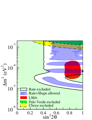
Figure 6: Left: KamLAND excluded regions of neutrino oscillation parameters $\mathsf{\Delta{m}^{2}}=\Delta{m}^{2}_{\mathrm{KamLAND}}$ and $\mathsf{\sin^{2}2\theta}=\sin^{2}2\vartheta_{\mathrm{KamLAND}}$ for the rate analysis and allowed regions for the combined rate and energy spectrum analysis at 95% C.L. At the top are the 95% C.L. excluded region from CHOOZ [84] and Palo Verde [85] experiments, respectively. The dark area is the 95% C.L. LMA allowed region obtained in Ref. [82]. The thick dot indicates the best fit of the KamLAND data in Eq. (2.36). Figure taken from Ref. [9]. Right: Allowed region at 90%, 95%, 99%, 99.73% ($3\sigma$) C.L. for the neutrino oscillation parameters $\mathsf{\Delta{m}^{2}}=\Delta{m}^{2}_{\mathrm{sol}}=\Delta{m}^{2}_{\mathrm{KamLAND}}$ and $\mathsf{\tan^{2}\theta}=\tan^{2}\vartheta_{\mathrm{sol}}=\tan^{2}\vartheta_{\mathrm{KamLAND}}$ obtained in Ref. [86] from the combined analysis of solar and KamLAND data (see also Refs. [87, 88, 89, 90, 91, 92, 93, 94]).

2.3 The first results of the KamLAND experiment

Recently the first results of the KamLAND experiment, started in January 2002, have been published [9]. In this experiment electron antineutrinos from many reactors in Japan and Korea are detected via the observation of the process

$$\bar{\nu}_{e}+p\to e^{+}+n\,.$$ (2.34)

The threshold energy of this process is $E_{\nu}^{\mathrm{th}}\simeq m_{e}+m_{n}-m_{p}=1.8\,\mathrm{MeV}$. About 80% of the $\bar{\nu}_{e}$ flux is expected from 26 reactors with distances in the range 138-214 km. The 1 kt liquid scintillator detector of the KamLAND experiment is located in the Kamioka mine, in Japan, at a depth of about 1 km. Both prompt photons from the annihilation of $e^{+}$ in the scintillator and 2.2 MeV delayed photons from the neutron capture $n+p\to d+\gamma$ are detected (the mean neutron capture time is $188\pm 23\,\mu\mathrm{sec}$). In order to avoid background, mainly from the decays of ${}^{238}\mathrm{U}$ and ${}^{232}\mathrm{Th}$ in the Earth, the cut $E_{\mathrm{prompt}}>2.6\,\mathrm{MeV}$ was applied.

During 145.1 days of running 54 events were observed. The number of events expected in the case of no neutrino oscillations is $86.8\pm 5.6$. The ratio of observed and expected $\bar{\nu}_{e}$ events is

$$\frac{N_{\mathrm{obs}}-N_{\mathrm{BG}}}{N_{\mathrm{expected}}}=0.611\pm 0.085\pm 0.041\,,$$ (2.35)

where $N_{\mathrm{BG}}=0.95\pm 0.99$ is the estimated number of background events.

The left figure in Fig. 5 shows the dependence of the ratio of observed and expected $\bar{\nu}_{e}$ events on the average distance between reactors and detectors for all reactor neutrino experiments. The dotted curve was obtained with the best-fit solar neutrino LMA values of the oscillation parameters $\Delta{m}^{2}_{\mathrm{sol}}=5.5\times 10^{-5}\,\mathrm{eV}^{2}$ and $\sin^{2}2\vartheta_{\mathrm{sol}}=0.83$ obtained in Ref. [82].

In the KamLAND experiment the prompt energy spectrum was also measured (see the right figure in Fig. 5). The prompt energy is connected with the energy of $\bar{\nu}_{e}$ by the relation $E_{\mathrm{prompt}}=E_{\bar{\nu}_{e}}-0.8\,\mathrm{MeV}-\overline{E_{n}}$ ($\overline{E_{n}}$ is the average kinetic energy of the neutron and $0.8\,\mathrm{MeV}=m_{n}-m_{p}-m_{e}$, with the electron neutrino mass coming from the annihilation of the final positron in Eq. (2.34) with an electron in the medium). From the two-neutrino analysis of the KamLAND spectrum the following best-fit values of the oscillation parameters were obtained:

$$\Delta{m}^{2}_{\mathrm{KamLAND}}=6.9\times 10^{-5}\mathrm{eV}^{2}\,,\qquad\sin^{2}2\vartheta_{\mathrm{KamLAND}}=1\,.$$ (2.36)

The 95% C.L. allowed regions in the plane of the oscillation parameters obtained from the analysis of the measured rate and energy spectrum are shown in the left figure in Fig. 6. The region outside the solid line is excluded from the rate analysis. The dark region is the solar neutrino LMA allowed region, obtained in Ref. [82]. One can see that two of the KamLAND allowed regions overlap with the solar neutrino LMA region.

The KamLAND result provides strong evidence of neutrino oscillations, obtained for the first time with terrestrial reactor antineutrinos with the initial flux well under control. The KamLAND result allows to exclude the SMA, LOW and VAC solutions of the solar neutrino problem. It proves that the only viable solution of the problem is LMA. The right figure in Fig. 6 shows the allowed region for the oscillation parameters obtained in Ref. [86] from the combined analysis of solar and KamLAND data (see also Refs. [87, 88, 89, 90, 91, 92, 93, 94]).

2.4 CHOOZ and Palo Verde

The results of the long-baseline reactor experiments CHOOZ [84] and Palo Verde [85], in which $\bar{\nu}_{e}$ disappearance due to neutrino oscillations in the atmospheric range of $\Delta{m}^{2}$ was searched for, are very important for the issue of neutrino mixing. In these experiments electron antineutrinos were detected via the observation of the process

$$\bar{\nu}_{e}+p\to e^{+}+n\,.$$ (2.37)

No indication in favor of the disappearance of reactor $\bar{\nu}_{e}$’s was found. The ratio $R$ of the measured and expected numbers of $\bar{\nu}_{e}$ events in the CHOOZ [84] and the Palo Verde [85] experiments are, respectively,

$$R=1.01\pm 2.8\%\pm 2.7\%\,,\qquad R=1.01\pm 2.4\%\pm 5.3\%\,.$$ (2.38)

From the 95% C.L. exclusion plot obtained in Ref. [84] from the two-neutrino analysis of CHOOZ data, for $\Delta{m}^{2}_{\mathrm{CHOOZ}}=2.5\times 10^{-3}\,\mathrm{eV}^{2}$ (the S-K best-fit value for $\Delta{m}^{2}_{\mathrm{atm}}$, see Eq. (2.17)) we have

$$\sin^{2}2\vartheta_{\mathrm{CHOOZ}}\lesssim 1.5\times 10^{-1}\,.$$ (2.39)

2.5 Phenomenology

In the minimal scheme with mixing of three massive neutrinos, the $3\times 3$ Pontecorvo-Maki-Nakagawa-Sakata [95, 96, 97] mixing matrix $U$ is characterized by three mixing angles and one CP phase (in the case of Dirac neutrinos; in the case of Majorana neutrinos, in the mixing matrix there are two additional phases which are irrelevant for neutrino oscillations). Let us discuss now neutrino oscillations in the atmospheric and solar ranges of neutrino mass-squared differences in the framework of this scheme, which provides two independent $\Delta{m}^{2}$’s: $\Delta{m}^{2}_{21}=m_{2}^{2}-m_{1}^{2}$ and $\Delta{m}^{2}_{32}=m_{3}^{2}-m_{2}^{2}$.

Two important features of the neutrino mixing, which were revealed in the recent solar, atmospheric, long-baseline reactor and accelerator experiments, determine neutrino oscillations.

The first feature is the hierarchy of the neutrino mass-squared differences: from the analyses of the data of the solar and atmospheric neutrino experiments it follows that $\Delta{m}^{2}_{\mathrm{sol}}\ll\Delta{m}^{2}_{\mathrm{atm}}$. This hierarchy can be realized only with the two types of three-neutrino mass schemes shown in Fig. 7. The absolute scale of the neutrino masses in the two schemes in Fig. 7 is not fixed by neutrino oscillation experiments. Figure 8 shows the neutrino masses as functions of the lightest mass $m_{1}$ (see Ref. [98]). One can see that the “normal” scheme in Fig. 7 is compatible with the natural mass hierarchy (2.7) if $m_{1}\ll m_{2}$, whereas in the “inverted” scheme $\nu_{2}$ and $\nu_{3}$ are always almost degenerate.

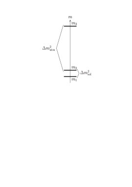
“normal”

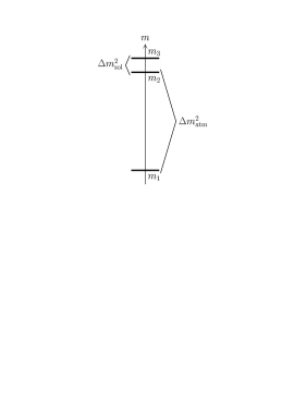
“inverted”

Figure 7: The two types of three-neutrino mass schemes compatible with the hierarchy $\Delta{m}^{2}_{\mathrm{sol}}\ll\Delta{m}^{2}_{\mathrm{atm}}$.

Let us first consider the “normal” mass scheme in Fig. 7, with $\Delta{m}^{2}_{21}\simeq\Delta{m}^{2}_{\mathrm{sol}}$ and $\Delta{m}^{2}_{32}\simeq\Delta{m}^{2}_{\mathrm{atm}}$. In this case we have

$$\Delta{m}^{2}_{21}\ll\Delta{m}^{2}_{32}\,.$$ (2.40)

For the values $L/E$ relevant for neutrino oscillations in the atmospheric range of $\Delta{m}^{2}$ (atmospheric and long-baseline accelerator and reactor experiments) we have $\Delta{m}^{2}_{21}L/E\ll 1$. Hence, we can neglect the contribution of $\Delta{m}^{2}_{21}$ to the transition probability in Eq. (2.11). For the probability of the transition $\nu_{\alpha}\to\nu_{\alpha^{\prime}}$, we obtain (see Ref. [19])

$$\mathrm{P}(\nu_{\alpha}\to\nu_{\alpha^{\prime}})=\frac{1}{2}\,\mathrm{A}_{{\alpha^{\prime}};\alpha}\left(1-\cos\Delta{m}^{2}_{32}\frac{L}{2E}\right)\qquad(\alpha\neq\alpha^{\prime})\,,$$ (2.41)

where the oscillation amplitude is given by

$$\mathrm{A}_{{\alpha^{\prime}};\alpha}=4\,|U_{\alpha^{\prime}3}|^{2}\,|U_{\alpha 3}|^{2}$$ (2.42)

In the standard parametrization of the mixing matrix (see Ref. [99]) we have

$$U_{e3}=\sin\vartheta_{13}\,e^{-i\delta}\,,\qquad U_{\mu 3}=\sqrt{1-|U_{e3}|^{2}}\,\sin\vartheta_{23}\,,\qquad U_{\tau 3}=\sqrt{1-|U_{e3}|^{2}}\,\cos\vartheta_{23}\,,$$ (2.43)

where $\vartheta_{13}$ and $\vartheta_{23}$ are mixing angles and $\delta$ is the CP-violating phase. Hence, for the amplitude of the transitions $\nu_{\mu}\to\nu_{\tau}$ and $\nu_{\mu}\to\nu_{e}$ we obtain, respectively,

$$\mathrm{A}_{\tau;\mu}=\left(1-|U_{e3}|^{2}\right)^{2}\sin^{2}2\vartheta_{23}\,,\qquad\mathrm{A}_{e;\mu}=4\,|U_{e3}|^{2}\left(1-|U_{e3}|^{2}\right)\sin^{2}\vartheta_{23}\,.$$ (2.44)

The probability of $\nu_{\alpha}$ to survive is given by

$$\mathrm{P}(\nu_{\alpha}\to\nu_{\alpha})=1-\sum_{\alpha^{\prime}\neq\alpha}\mathrm{P}(\nu_{\alpha}\to\nu_{\alpha^{\prime}})=1-\frac{1}{2}\,\mathrm{B}_{\alpha;\alpha}\left(1-\cos\Delta{m}^{2}_{32}\frac{L}{2E}\right)\,.$$ (2.45)

where

$$\mathrm{B}_{\alpha;\alpha}=\sum_{\alpha^{\prime}\neq\alpha}\,\mathrm{A}_{{\alpha^{\prime}};\alpha}=4\,|U_{\alpha 3}|^{2}\left(1-|U_{\alpha 3}|^{2}\right)\,.$$ (2.46)

Thus, due to the hierarchy in Eq. (2.40), the transition probabilities in the atmospheric range of $\Delta{m}^{2}$ have a two-neutrino form. Taking into account that the elements $|U_{\alpha 3}|^{2}$, which determine the oscillation amplitudes, satisfy the unitarity condition $\sum_{\alpha}|U_{\alpha 3}|^{2}=1$, we conclude that the transition probabilities are characterized by three parameters: $\Delta{m}^{2}_{32}$, $\sin^{2}2\vartheta_{23}$ and $|U_{e3}|^{2}$.

“normal”

“inverted”

Figure 8: Neutrino masses as functions of the lightest mass $m_{1}$ in the two three-neutrino mass schemes in Fig. 7. The dashed and dotted lines represent, respectively, the limits for $m_{2}$ and $m_{3}$ from solar and atmospheric neutrino data.

Let us consider now neutrino oscillations in the solar range of $\Delta{m}^{2}$. The $\nu_{e}$ survival probability in vacuum can be written in the form

$$\mathrm{P}(\nu_{e}\to\nu_{e})=\left|\sum_{i=1,2}|U_{ei}|^{2}\,e^{-i\,\Delta{m}^{2}_{i1}\frac{L}{2E}}+|U_{e3}|^{2}\,e^{-i\,\Delta{m}^{2}_{31}\frac{L}{2E}}\,\right|^{2}$$ (2.47)

We are interested in the survival probability averaged over the region where neutrinos are produced, over the detector energy resolution, etc.. Because of the neutrino mass-squared hierarchy in Eq. (2.40), in the expression for the averaged survival probability the interference between the first and second terms in (2.47) vanishes and we obtain

$$\mathrm{P}(\nu_{e}\to\nu_{e})=|U_{e3}|^{4}+\left(1-|U_{e3}|^{2}\right)^{2}P^{(1,2)}(\nu_{e}\to\nu_{e})\,,$$ (2.48)

where

$$\mathrm{P}^{(1,2)}(\nu_{e}\to\nu_{e})=1-\frac{1}{2}\,A^{(1,2)}\left(1-\cos\Delta{m}^{2}_{21}\frac{L}{2E}\right)\,,$$ (2.49)

and

$$A^{(1,2)}=4\,\frac{|U_{e1}|^{2}\,|U_{e2}|^{2}}{\left(1-|U_{e3}|^{2}\right)^{2}}=\sin^{2}2\vartheta_{12}\,.$$ (2.50)

We have used the standard parametrization of the neutrino mixing matrix (see Eq. (2.43) and Ref. [99]), with

$$U_{e1}=\sqrt{1-|U_{e3}|^{2}}\,\cos\vartheta_{12}\,,\qquad U_{e2}=\sqrt{1-|U_{e3}|^{2}}\,\sin\vartheta_{12}\,,$$ (2.51)

where $\vartheta_{12}$ is a mixing angle. The expression (2.48) is also valid in the case of oscillations in matter [100]. In this case $P^{(1,2)}(\nu_{e}\to\nu_{e})$ is the two-neutrino survival probability in matter calculated with the charged-current matter potential $V_{\mathrm{CC}}$ multiplied by $(1-|U_{e3}|^{2})$.

The second important feature of the neutrino mixing is the smallness of the parameter $|U_{e3}|^{2}$. This follows from the results of the CHOOZ and Palo Verde experiments and from the results of solar neutrino experiments. In the CHOOZ and Palo Verde experiments, the probability of $\bar{\nu}_{e}$ to survive is

$$\mathrm{P}(\bar{\nu}_{e}\to\bar{\nu}_{e})=1-\frac{1}{2}\,\mathrm{B}_{e;e}\left(1-\cos\Delta{m}^{2}_{32}\frac{L}{2E}\right)\,,$$ (2.52)

where

$$\mathrm{B}_{e;e}=4\,|U_{e3}|^{2}\left(1-|U_{e3}|^{2}\right)\,.$$ (2.53)

From the two-neutrino exclusion plots, obtained in the CHOOZ and Palo Verde experiments [84, 85], it follows that

$$\mathrm{B}_{e;e}\leq\mathrm{B}_{e;e}^{0}\,,$$ (2.54)

where the upper bound $\mathrm{B}_{e;e}^{0}$ depends on $\Delta{m}^{2}_{32}$.

For the S-K [1, 2, 3] allowed values of $\Delta{m}^{2}_{32}$, from the 95% C.L. CHOOZ exclusion plot we find

$$1\times 10^{-1}\lesssim\mathrm{B}_{e;e}^{0}\lesssim 2.4\times 10^{-1}\,.$$ (2.55)

Thus, the parameter $|U_{e3}|^{2}$ can be small or large (close to one). This last possibility is excluded by the solar neutrino data (see [19]). At the S-K best-fit point $\Delta{m}^{2}_{32}=2.5\times 10^{-3}\mathrm{eV}^{2}$ we have

$$|U_{e3}|^{2}\leq 4\times 10^{-2}\qquad(95\%\,\mathrm{C.L.})\,.$$ (2.56)

A combined fit of all data leads to [83]

$$|U_{e3}|^{2}\leq 5\times 10^{-2}\qquad(99.73\%\,\mathrm{C.L.})\,.$$ (2.57)

There are three major consequences of the neutrino mass-squared hierarchy (2.40) and of the smallness of $|U_{e3}|^{2}$:

1. The dominant transition in the atmospheric range of $\Delta{m}^{2}$ is $\nu_{\mu}\to\nu_{\tau}$. From Eq. (2.44) it follows that

   $$\Delta{m}^{2}_{32}\simeq\Delta{m}^{2}_{\mathrm{atm}}\,,\qquad\sin^{2}2\vartheta_{23}\simeq\sin^{2}2\vartheta_{\mathrm{atm}}\,.$$ (2.58)

2. In the solar range of $\Delta{m}^{2}$ the probability of $\nu_{e}$ to survive has the two-neutrino form

   $$\mathrm{P}(\nu_{e}\to\nu_{e})\simeq\mathrm{P}^{(1,2)}(\nu_{e}\to\nu_{e})\,.$$ (2.59)

   From Eqs. (2.49) and (2.50) it follows that

   $$\Delta{m}^{2}_{21}\simeq\Delta{m}^{2}_{\mathrm{sol}}\,,\qquad\tan^{2}\vartheta_{12}\simeq\tan^{2}\vartheta_{\mathrm{sol}}\,.$$ (2.60)

3. Neutrino oscillations in the atmospheric and solar ranges of $\Delta{m}^{2}$ in the leading approximation are decoupled [101]. Oscillations in both ranges are described by two-neutrino formulas, which are characterized, respectively, by the parameters $\Delta{m}^{2}_{32}$, $\sin^{2}2\vartheta_{23}$ and $\Delta{m}^{2}_{21}$, $\tan^{2}\vartheta_{12}$.

We have considered the hierarchy (2.40) of the neutrino mass-squared differences, which is realized in the “normal” mass scheme in Fig. 7. The data of neutrino oscillation experiments are compatible also with the “inverted” mass scheme in Fig. 7, with $\Delta{m}^{2}_{21}\simeq\Delta{m}^{2}_{\mathrm{atm}}$ and $\Delta{m}^{2}_{32}\simeq\Delta{m}^{2}_{\mathrm{sol}}$. In this case an inverted hierarchy of the mass-squared differences takes place:

$$\Delta{m}^{2}_{32}\ll\Delta{m}^{2}_{21}$$ (2.61)

The expressions for the transition probabilities in the case of the inverted hierarchy can be obtained from Eqs. (2.41), (2.42), (2.45), (2.46), (2.48)-(2.50) with the change $\Delta{m}^{2}_{32}\leftrightarrows\Delta{m}^{2}_{21}$, $|U_{\alpha 3}|^{2}\leftrightarrows|U_{\alpha 1}|^{2}$, $\vartheta_{12}\leftrightarrows\vartheta_{23}$, $P^{(1,2)}\to P^{(2,3)}$, $A^{(1,2)}\to A^{(2,3)}$.

We have discussed up to now evidences in favor of neutrino oscillations that have been obtained in the atmospheric and solar neutrino experiments. There exist at present also an indication in favor of short-baseline $\bar{\nu}_{\mu}\to\bar{\nu}_{e}$ transitions, which has been obtained only in the accelerator experiment LSND [21]. The LSND data can be explained by neutrino oscillations. From a two-neutrino analysis of the data, the best-fit values of the oscillation parameters are

$$\Delta{m}^{2}_{\mathrm{LSND}}\simeq 1.2\,\mathrm{eV}^{2}\,,\qquad\sin^{2}2\vartheta_{\mathrm{LSND}}\simeq 3\times 10^{-3}\,.$$ (2.62)

In order to describe the results of the solar, atmospheric and LSND experiments, which require three different values of neutrino mass-squared differences $\Delta{m}^{2}_{\mathrm{sol}}$, $\Delta{m}^{2}_{\mathrm{atm}}$ and $\Delta{m}^{2}_{\mathrm{LSND}}$, it is necessary to assume that at least one sterile neutrino exists in addition to the three active neutrinos $\nu_{e}$, $\nu_{\mu}$, $\nu_{\tau}$. In the mass basis, in addition to the three light neutrinos $\nu_{1}$, $\nu_{2}$, $\nu_{3}$ there must be at least one neutrino with mass of the order $\sqrt{\Delta{m}^{2}_{\mathrm{LSND}}}\simeq 1\,\mathrm{eV}$ (see, for example, Ref. [19]). However, in spite of the additional degrees of freedom, schemes with four neutrinos do not fit well the data (see Refs. [102, 103]).

The result of the LSND experiment requires, however, confirmation. The MiniBooNE experiment at Fermilab [104], that started recently, is aimed to check the LSND result.

From neutrino oscillation experiments we can obtain information only on the neutrino mass-squared differences, not on the absolute values of neutrino masses. The great advantage of neutrino oscillations experiments, that was stressed in the early papers on neutrino oscillations [95, 96, 105], is that they are sensitive to very small values of $\Delta{m}^{2}$. This is connected with the fact that neutrino oscillations are an interference phenomenon. It is also important that there is the possibility to perform experiments with detectors at very large distances from neutrino sources (solar, atmospheric and long-baseline experiments) and for small neutrino energies (solar and reactor experiments).

The understanding of the origin of neutrino masses and neutrino mixing requires knowledge of the absolute values of neutrino masses (see Refs. [61, 60]). The problem of the absolute values of neutrino masses is one of the most challenging problems of the physics of massive and mixed neutrinos. At present there are only upper bounds for the absolute values of neutrino masses. The most stringent bound was obtained from the experiments on the measurement of the high energy part of the $\beta$-spectrum of ${}^{3}\mathrm{H}$. In the next section we will discuss the results of these experiments and future prospects.

3 Neutrino mass from $\beta$-decay experiments

3.1 The $\beta$-spectrum in the case of neutrino mixing

The method of measurement of the neutrino mass through the detailed investigation of the high-energy part of the $\beta$-spectrum was proposed in 1934 by Fermi in his classical paper on the theory of $\beta$-decay [106] and by Perrin [107]. The first experiments on the measurement of the neutrino mass with this method have been done in 1948-49 [108, 109].

Usually, the neutrino mass is measured through the measurement of the high energy part of the $\beta$-spectrum of tritium

$${}^{3}\mathrm{H}\to{}^{3}\mathrm{He}+e^{-}+\bar{\nu}_{e}\,.$$ (3.1)

The investigation of this decay has several advantages. Since tritium decay is superallowed, the nuclear matrix element is a constant and the electron spectrum is determined by the phase space. It has a relatively small energy release $E_{0}\simeq 18.6\,\mathrm{keV}$ and a convenient lifetime ($T_{1/2}\simeq 12.3$ years). A small value of $E_{0}$ is convenient because the relative fraction of events in the high energy part of the spectrum, which is sensitive to the neutrino mass, is proportional to $E_{0}^{-3}$.

Let us consider the decay (3.1) in the case of nonzero neutrino masses and neutrino mixing. The effective Hamiltonian of the process is

$$\mathcal{H}_{I}^{\mathrm{CC}}=\frac{G_{F}}{\sqrt{2}}\,2\,\bar{e}_{L}\gamma_{\alpha}\nu_{eL}\,j^{\alpha}+\mathrm{h.c.}\,,$$ (3.2)

where $j^{\alpha}$ is the hadronic charged current and the field $\nu_{eL}$ is given by (see Eq. (2.2))

$$\nu_{eL}=\sum_{i}U_{ei}\nu_{iL}\,.$$ (3.3)

The state of the final particles in the decay (3.1) is

$$|f\rangle=\sum_{i}|P^{\prime}\rangle\,|p\rangle\,|p_{i}\rangle\,U^{*}_{ei}\,\langle p,p_{i},P^{\prime}|(S-1)|P\rangle\,.$$ (3.4)

Here $p$ is the momentum of the electron, $P$ and $P^{\prime}$ are the momenta of the initial and final nuclei, $p_{i}$ is the antineutrino momentum, $|P^{\prime}\rangle$, $|p\rangle$, $|p_{i}\rangle$ are the normalized states of the final nucleus, electron, antineutrino with mass $m_{i}$, and

$$\langle p,p_{i},P^{\prime}|(S-1)|P\rangle=\langle p,p_{i},P^{\prime}|T|P\rangle\,(2\pi)^{4}\,\delta^{4}(p+p_{i}+P^{\prime}-P)$$ (3.5)

is the element of the $S$-matrix.

We are interested in the spectrum of electrons. After the integration over the momenta $\vec{P^{\prime}}$, $\vec{p_{i}}$ and over the angle of emission of the electron, we have

$$\frac{\mathrm{d}\Gamma}{\mathrm{d}E}=\sum_{i}|U_{ei}|^{2}\,\frac{\mathrm{d}\Gamma_{i}}{\mathrm{d}E}\,,$$ (3.6)

where

$$\frac{\mathrm{d}\Gamma_{i}}{\mathrm{d}E}=C\,p\,(E+m_{e})\,(E_{0}-E)\,\sqrt{(E_{0}-E)^{2}-m_{i}^{2}}\,F(E)\,\theta(E_{0}-E-m_{i})\,.$$ (3.7)

Here $E$ is the kinetic energy of the electron, $E_{0}$ is the energy released in the decay, $m_{e}$ is the mass of the electron and $F(E)$ is the Fermi function, which describes the Coulomb interaction of the final particles. The constant $C$ is given by

$$C=G_{F}^{2}\frac{m_{e}^{5}}{2\,\pi^{3}}\,\cos^{2}\theta_{C}\,|M|^{2}\,,$$ (3.8)

where $G_{F}$ is the Fermi constant, $\theta_{C}$ is the Cabibbo angle, $M$ is the nuclear matrix element (a constant).

Let us notice that neutrino masses enter in the expression (3.7) through the neutrino momentum $|\vec{p}_{i}|=\sqrt{(E_{0}-E)^{2}-m_{i}^{2}}$. The step function $\theta(E_{0}-E-m_{i})$ provides the condition $E\leq E_{0}-m_{i}$. The recoil of the final nucleus was neglected in Eq. (3.7).

Two experiments on the measurement of neutrino masses with the tritium method are going on at present (Mainz [31, 32, 33] and Troitsk [34, 35]). The sensitivity of these experiments to the neutrino mass is about 2-3 eV. The sensitivity to the neutrino mass of the future experiment KATRIN [36] is expected to be about one order of magnitude better (0.35 eV). We will discuss the results of the Mainz and Troitsk experiments later. Now we consider the possibility to determine the neutrino mass from the results of the $\beta$-decay experiments for different neutrino mass spectra, having in mind these sensitivities.

As it is seen from Eq. (3.7), the largest distortion of the $\beta$-spectrum due to neutrino masses can be observed in the region

$$E_{0}-E\simeq m_{i}\,.$$ (3.9)

However, for $m_{i}\simeq 1\,\mathrm{eV}$ only a very small part (about $10^{-13}$) of the decays of tritium give contribution to the region (3.9). This is the reason why in the analysis of the results of the measurement of the tritium $\beta$-spectrum a relatively large part of the spectrum is used (for example, in the Mainz experiment the last 70 eV of the spectrum). Taking this into account, the tritium $\beta$-spectrum that is used for the fit of the data can be presented in the form [110, 111, 31, 112, 113] (see also the discussion in Ref. [114])

$$\frac{\mathrm{d}\Gamma}{\mathrm{d}E}=C\,p\,(E+m_{e})\,(E_{0}-E)\,\sqrt{(E_{0}-E)^{2}-m_{\beta}^{2}}\,F(E)\,,$$ (3.10)

where the effective mass $m_{\beta}$ is given by

$$m^{2}_{\beta}=\sum_{i}|U_{ei}|^{2}\,m^{2}_{i}$$ (3.11)

Let us consider first the minimal scheme with three massive neutrinos $\nu_{1}$, $\nu_{2}$ and $\nu_{3}$. The minimal neutrino mass $m_{1}$ and the character (“normal” or “inverted”, hierarchical or almost degenerate) of the neutrino mass spectrum are unknown at present. Neutrino oscillation experiments allow to determine the neutrino mass-squared differences $\Delta{m}^{2}_{21}$ and $\Delta{m}^{2}_{32}$. Hence, it is possible to express the values of the neutrino masses $m_{2}$ and $m_{3}$ in terms of the unknown mass $m_{1}$ as

$$m_{2}=\sqrt{m^{2}_{1}+\Delta{m}^{2}_{21}}\,,\qquad m_{3}=\sqrt{m^{2}_{1}+\Delta{m}^{2}_{21}+\Delta{m}^{2}_{32}}\,.$$ (3.12)

In the “normal” three-neutrino scheme in Fig. 7, $\Delta{m}^{2}_{21}=\Delta{m}^{2}_{\mathrm{sol}}$ and $\Delta{m}^{2}_{32}=\Delta{m}^{2}_{\mathrm{atm}}$. Using Eqs. (2.51) and (2.60), we obtain

$$m_{\beta}^{2}=m_{1}^{2}+\left(\sin^{2}\vartheta_{\mathrm{sol}}+\cos^{2}\vartheta_{\mathrm{sol}}\,|U_{e3}|^{2}\right)\Delta{m}^{2}_{\mathrm{sol}}+|U_{e3}|^{2}\,\Delta{m}^{2}_{\mathrm{atm}}\,.$$ (3.13)

In the case of the natural neutrino mass hierarchy (2.7), we have

$$m_{2}\simeq\sqrt{\Delta{m}^{2}_{\mathrm{sol}}}\simeq 7\times 10^{-3}\,\mathrm{eV}\,,\qquad m_{3}\simeq\sqrt{\Delta{m}^{2}_{\mathrm{atm}}}\simeq 5\times 10^{-2}\,\mathrm{eV}\,,$$ (3.14)

where the best-fit values (2.17) and (2.33) of the oscillation parameters were used.

The contribution of the heaviest neutrino mass $m_{3}$ to the effective neutrino mass (3.11) enters with the weight $|U_{e3}|^{2}$, for which we have the upper bound (2.57) from the results of the CHOOZ experiment [84]. Taking into account this bound and using the best-fit value in Eq. (2.33) for $\vartheta_{\mathrm{sol}}$, for the effective neutrino mass $m_{\beta}$ we obtain

$$m_{\beta}\simeq\left(\sin^{2}\vartheta_{\mathrm{sol}}\,\Delta{m}^{2}_{\mathrm{sol}}+|U_{e3}|^{2}\,\Delta{m}^{2}_{\mathrm{atm}}\right)^{1/2}\lesssim 1.2\times 10^{-2}\mathrm{eV}\,,$$ (3.15)

which is about one order of magnitude smaller than the sensitivity of the future tritium experiment KATRIN [36].

In the “inverted” three-neutrino scheme in Fig. 7, with $\Delta{m}^{2}_{21}=\Delta{m}^{2}_{\mathrm{atm}}$ and $\Delta{m}^{2}_{32}=\Delta{m}^{2}_{\mathrm{sol}}$, using Eq. (2.51), we obtain

$$m_{\beta}^{2}=m_{1}^{2}+\left(1-|U_{e1}|^{2}\right)\left(\Delta{m}^{2}_{\mathrm{atm}}+\sin^{2}\vartheta_{\mathrm{sol}}\,\Delta{m}^{2}_{\mathrm{sol}}\right)\,.$$ (3.16)

The value of $|U_{e1}|^{2}$ in the “inverted” neutrino scheme is bounded by the results of the CHOOZ experiment as the value of $|U_{e3}|^{2}$ in the “normal” neutrino scheme (see Eq. (2.57) and the remark after Eq. (2.61)):

$$|U_{e1}|^{2}\leq 5\times 10^{-2}\qquad(99.73\%\,\mathrm{C.L.})\,.$$ (3.17)

In the case of the “inverted” neutrino mass hierarchy $m_{1}\ll m_{2}<m_{3}$ we have

$$m_{2}\simeq m_{3}\simeq\sqrt{\Delta{m}^{2}_{\mathrm{atm}}}\simeq 5\times 10^{-2}\,\mathrm{eV}\,,\qquad m_{1}\ll\sqrt{\Delta{m}^{2}_{\mathrm{atm}}}\,.$$ (3.18)

For the effective neutrino mass $m_{\beta}$ we obtain

$$m_{\beta}\simeq\sqrt{\Delta{m}^{2}_{\mathrm{atm}}}\simeq 5\times 10^{-2}\,\mathrm{eV}\,,$$ (3.19)

which is also much smaller than the sensitivity of the KATRIN experiment.

“normal”

“inverted”

Figure 9: Value of $m_{\beta}$ as a function of $m_{1}$ (see Eqs. (3.13) and (3.16)). The two dashed curves have been calculated assuming the best-fit values of $\Delta{m}^{2}_{\mathrm{sol}}$ and $\vartheta_{\mathrm{sol}}$ in Eq. (2.33) and the best-fit value of $\Delta{m}^{2}_{\mathrm{atm}}$ in Eq. (2.17). The lower dashed curves correspond to $|U_{e3}|^{2}=0$ in the “normal” scheme and $|U_{e1}|^{2}=0$ in the “inverted” scheme. The upper dashed curves correspond to the upper limits $|U_{e3}|^{2}=5\times 10^{-2}$ (Eq. (2.57)) in the “normal” scheme and $|U_{e1}|^{2}=5\times 10^{-2}$ (Eq. (3.17)) in the “normal” scheme. The two solid curves represent the lower and upper limits for $m_{\beta}$ obtained from the 99.73% C.L. solar LMA-MSW region in Ref. [77] and the 99% C.L. atmospheric region in Ref. [115], and $|U_{e3}|^{2}$ and $|U_{e1}|^{2}$ bounded by Eqs. (2.57) and (3.17), respectively, in the “normal” and “inverted” schemes.

Figure 9 shows the allowed values of $m_{\beta}$ as a function of $m_{1}$. One can see that in both the “normal” and “inverted” three-neutrino schemes in Fig. 7, the KATRIN experiment may obtain a positive result only if the three neutrino masses are almost degenerate and $m_{1}$ is of the same order or larger than the sensitivity of the experiment ($m_{1}\gtrsim 0.3\,\mathrm{eV}$). In this case $m_{1}\simeq m_{2}\simeq m_{3}$, and from the unitarity of the mixing matrix we obtain

$$m_{\beta}\simeq m_{1}\,,$$ (3.20)

as shown in Fig. 9.

If the LSND result [21] is confirmed by the MiniBooNE [104] experiment, it will mean that (at least) four massive and mixed neutrinos exist in nature.

Let us discuss now the possibilities to measure the neutrino mass with the tritium method in the case of four massive neutrinos. In this case, we have three different neutrino mass-squared differences $\Delta{m}^{2}_{\mathrm{sol}}$, $\Delta{m}^{2}_{\mathrm{atm}}$ and $\Delta{m}^{2}_{\mathrm{LSND}}$, given by (2.17), (2.33) and (2.62). Let us assume that $m_{1}\ll\sqrt{\Delta{m}^{2}_{\mathrm{LSND}}}$.

Figure 10: The six allowed types of four-neutrino mass schemes.

Figure 10 shows the six four-neutrino mass spectra compatible with the mass-squared hierarchy $\Delta{m}^{2}_{\mathrm{sol}}\ll\Delta{m}^{2}_{\mathrm{atm}}\ll\Delta{m}^{2}_{\mathrm{LSND}}$. In all spectra there are two groups of close masses, separated by the LSND gap of the order of 1 eV. There are two possibilities for the groups: 2+2 and 3+1.

In order to calculate the contribution of neutrino masses to the $\beta$-spectrum it is necessary to take into account the constraints on the elements of the neutrino mixing matrix that can be obtained from the data of the short-baseline reactor experiment Bugey [116], in which no indication in favor of neutrino oscillations was found.

In the framework of four-neutrino mixing, the probability of the reactor $\bar{\nu}_{e}$’s to survive is given by (see [19])

$$\mathrm{P}(\bar{\nu}_{e}\to\bar{\nu}_{e})=1-\frac{1}{2}\mathrm{B}_{e;e}\left(1-\cos\Delta{m}^{2}_{41}\frac{L}{2E}\right)\,.$$ (3.21)

Here

$$\mathrm{B}_{e;e}=4\,\sum_{i}|U_{ei}|^{2}\left(1-\sum_{i}|U_{ei}|^{2}\right)\,,$$ (3.22)

where $i$ runs over the mass indices of the first (or second) group.

From the exclusion curve obtained in the Bugey experiment [116], we have

$$\mathrm{B}_{e;e}\leq\mathrm{B}^{0}_{e;e},$$ (3.23)

where the upper bound $\mathrm{B}^{0}_{e;e}$ depends on $\Delta{m}^{2}_{41}$.

Let us consider first the neutrino mass spectra I, II and B in Fig. 10, in which the solar neutrino mass-squared difference $\Delta{m}^{2}_{\mathrm{sol}}$ belongs to the light group. Taking into account the solar neutrino data, from the Bugey exclusion plot [116] we obtain

$$\sum_{i}|U_{ei}|^{2}\lesssim 2\times 10^{-2}\,,$$ (3.24)

where $i$ runs over indices of neutrinos belonging to the heavy group ($i=3,4$ for 2+2 scheme and $i=4$ for 3+1 schemes). Thus, in this case the contribution of heavy neutrinos to the $\beta$ spectrum is suppressed. For the effective neutrino mass we have the upper bound

$$m_{\beta}\lesssim\left(\sum_{i}|U_{ei}|^{2}\,\Delta{m}^{2}_{\mathrm{LSND}}+\Delta{m}^{2}_{\mathrm{atm}}\right)^{1/2}\,.$$ (3.25)

Taking into account (3.24) and using the best fit values of the parameters $\Delta{m}^{2}_{\mathrm{LSND}}$ and $\Delta{m}^{2}_{\mathrm{atm}}$ (see (2.17) and (2.62)), for the effective neutrino mass $m_{\beta}$ we obtain the bound

$$m_{\beta}\lesssim 1.6\times 10^{-1}\mathrm{eV}\,,$$ (3.26)

which is smaller than the sensitivity of the future tritium experiment KATRIN.

If $\Delta{m}^{2}_{\mathrm{sol}}$ is the mass-squared difference of neutrinos belonging to the heavy group, in Eq. (3.22) the index $i$ takes the values $i=1,2$ for 2+2 scheme and $i=1$ for 3+1 schemes.

In this case, taking into account the unitarity of the mixing matrix, we have

$$m_{\beta}\simeq\sqrt{\Delta{m}^{2}_{\mathrm{LSND}}}\,.$$ (3.27)

The allowed range for the parameter $\Delta{m}^{2}_{\mathrm{LSND}}$ found in Ref. [21] is (see also Ref. [117])

$$0.2\,\mathrm{eV}^{2}\lesssim\Delta{m}^{2}_{\mathrm{LSND}}\lesssim 2\,\mathrm{eV}^{2}\,.$$ (3.28)

From Eqs. (3.27) and (3.28), for the effective neutrino mass we have the limits

$$0.45\,\mathrm{eV}\lesssim m_{\beta}\lesssim 1.4\,\mathrm{eV}\,.$$ (3.29)

In this case, if the data of the LSND experiment are confirmed by the MiniBooNE experiment, there is a chance to observe the effect of neutrino mass in the future KATRIN experiment [36] with the expected sensitivity of about 0.35 eV.

3.2 Mainz experiment

The source in the Mainz experiment [31, 32, 33] is frozen molecular tritium condensed on a graphite substrate. The spectrum of the electron is measured by an integral MAC-E-Filter spectrometer (Magnetic Adiabatic Collimator with a retarding Electrostatic filter). This spectrometer combines high luminosity with high resolution. The resolution of the spectrometer is $4.8\,\mathrm{eV}$. In the analysis of the experimental data four variable parameters are used: the normalization $C$, the background $B$, the released energy $E_{0}$ and the effective neutrino mass-squared $m^{2}_{\beta}$. From the fit of the data it was found that $E_{0}=18.575\,\mathrm{keV}$.

The left figure in Fig. 11 shows the integral spectrum, measured in 1994, in 1998-1999, and in 2001, as a function of the retarding energy near the endpoint $E_{0}$, and the effective endpoint $E_{0,\mathrm{eff}}$. The position of $E_{0,\mathrm{eff}}$ takes into account the width of the response function of the setup and the mean rotation-vibration excitation energy of the electronic ground state of the $\mathrm{{}^{3}HeT^{+}}$ daughter molecule. The solid curve was obtained from the fit of the data under the assumption $m_{\beta}=0$. Different parts of the spectrum were used in the analysis of the data. The right figure in Fig. 11 shows the dependence of $m^{2}_{\beta}$ on the lower limit $E_{\mathrm{low}}$ of the corresponding fit interval (the upper limit is fixed at 18.66 keV, well above $E_{0}$) for data from 1998 and 1999 (open circles) and from the last runs of 2001 (filled circles). The error bars show the statistical uncertainties (inner bar) and the total uncertainty (outer bar). The correlation of data points for large fit intervals is due to the uncertainties of the systematic corrections, which are dominant for fit intervals with a lower boundary $E_{\mathrm{low}}<18.5\,\mathrm{keV}$.

Figure 11: Left: Integral spectrum measured in 1994 (open circles), 1998/1999 (filled squares) with fit (line) and 2001 (open squares) in the Mainz experiment. Right: Mainz fit results on $m^{2}_{\nu}\equiv m^{2}_{\beta}$ as a function of the lower boundary $E_{\mathrm{low}}$ of the fit interval for data from 1998 and 1999 (open circles) and from 2001 (filled circles). Figures taken from Ref. [33].

In the last $70\,\mathrm{eV}$ of the spectrum the combined statistical and systematical error is minimal. From the fit of the 1998-1999 experimental data in this interval, it was found that

$$m^{2}_{\beta}=(-1.6\pm 2.5\pm 2.1)\,\mathrm{eV}^{2}\,,$$ (3.30)

which corresponds to the upper bound

$$m_{\beta}<2.2\,\mathrm{eV}\qquad(95\%\,\mathrm{C.L.})\,.$$ (3.31)

In 2001 additional measurements of the $\beta$-decay spectrum were carried on by the Mainz group. From the analysis of these data it was obtained [33]

$$m^{2}_{\beta}=(0.1\pm 4.2\pm 2.0)\,\mathrm{eV}^{2}\,.$$ (3.32)

From the combined analysis of 1998, 1999 and 2001 data it was found [33]

$$m^{2}_{\beta}=(-1.2\pm 2.2\pm 2.1)\,\mathrm{eV}^{2}\,.$$ (3.33)

This value corresponds again to the upper bound [33]

$$m_{\beta}<2.2\,\mathrm{eV}\qquad(95\%\,\mathrm{C.L.})\,,$$ (3.34)

showing that the Mainz experiment has reached his sensitivity limit.

3.3 Troitsk experiment

In the Troitsk neutrino experiment [34, 35], as in the Mainz experiment, an integral electrostatic spectrometer with a strong inhomogeneous magnetic field, focusing the electrons, is used. The resolution of the spectrometer is $3.5-4$ eV. An important difference between the Troitsk and Mainz experiments is that in the Troitsk experiment the tritium source is a gaseous molecular source. Such a source has important advantages in comparison with the frozen source: there is no backscattering, there are no effects of the self-charging, the interaction between tritium molecules can be neglected, etc.. In the analysis of the data the same four variable parameters $C$, $B$, $E_{0}$ and $m^{2}_{\beta}$ were used. From the fit of the data, for the parameter $m^{2}_{\beta}$ large negative values in the range $-20\div-10\,\mathrm{eV}^{2}$ have been obtained. The investigation of the character of the measured spectrum suggests that the negative $m^{2}_{\beta}$ is due to a step function superimposed on the integral continuous spectrum. The step function in the integral spectrum corresponds to a narrow peak in the differential spectrum.

In order to describe the data, the authors of the Troitsk experiment added to the theoretical integral spectrum a step function with two additional variable parameters (position of the step $E_{\mathrm{step}}$ and the height of the step). From a six-parameter fit of the data, the Troitsk Collaboration found

$$m^{2}_{\beta}=(-2.3\pm 2.5\pm 2.0)\,\mathrm{eV}^{2}\,.$$ (3.35)

This value corresponds to the upper bound

$$m_{\beta}<2.2\,\mathrm{eV}\qquad(95\%\,\mathrm{C.L.})\,,$$ (3.36)

as in the Mainz experiment.

The Troitsk Collaboration found that the position of the step $E_{0}-E_{\mathrm{step}}$ changes periodically in the interval $5-15$ eV and that the average value of the height of the step is about $6\times 10^{-11}$ of the total number of events. This effect has been called “Troitsk anomaly”. Since the Mainz data do not show any indication of a Troitsk-like anomaly, it is believed [33] that the Troitsk anomaly is caused by some experimental artifact.

3.4 Other experiments

We have discussed up to now tritium experiments for the measurement of the neutrino mass. The groups in Genova [118] and Milano [119] are developing low temperature cryogenic detectors for the measurement of the $\beta$-decay spectrum of ${}^{187}\mathrm{Re}$. This element has the lowest known energy release ($E_{0}=2.5\,\mathrm{keV}$). The relative fraction of events in the high energy part of the spectrum is proportional to $E_{0}^{-3}$. Thus, decays with low $E_{0}$ values are very suitable for calorimetric experiments in which the full spectrum is measured. The limit for the neutrino mass that was obtained by the Genova group in Ref. [118] is

$$m_{\beta}<26\,\mathrm{eV}\qquad(95\%\,\mathrm{C.L.})\,.$$ (3.37)

In the future a sensitivity of about $10\,\mathrm{eV}$ is expected to be reached.

3.5 The future KATRIN experiment

In the future tritium experiment KATRIN [36], two tritium sources will be used: a gaseous molecular source ($\mathrm{T}_{2}$), as in the Troitsk experiment, and a frozen tritium source, as in the Mainz experiment. The windowless gaseous tritium source will allow to reach a column density $5\times 10^{17}\,\mathrm{T}_{2}/\mathrm{cm}^{2}$.

The integral MAC-E-Filter spectrometer will have two parts: the pre-spectrometer, which will select electrons in the last part (about 100  eV) of the spectrum, and the main spectrometer. This spectrometer will have a resolution of 1 eV.

It is planned that the KATRIN experiment will start to collect data in 2007. After three years of running the accuracy in the measurement of the parameter $m^{2}_{\beta}$ will be $0.08\,\mathrm{eV}^{2}$. This will allow to reach a sensitivity of 0.35 eV in the determination of the effective neutrino mass $m_{\beta}$.

As in the case of the Mainz experiment, in the analysis of the data of the future KATRIN experiment four variable parameters are planned to be used. The value of the parameter $E_{0}$ can be taken, however, from the independent measurement of the ${}^{3}\mathrm{H}$ and ${}^{3}\mathrm{He}$ mass difference. If the accuracy of such measurements reaches 1 p.p.m., the sensitivity of the KATRIN experiment to the neutrino mass will be significantly improved.

In the KATRIN experiment, not only the integral spectrum, but also the differential spectrum is planned to be measured. These measurements will allow to clarify the problem of the Troitsk anomaly in a direct way.

4 Muon and tau neutrino mass measurements

Information on the “mass” of the muon neutrino can be obtained from the measurement of the muon momentum in the decay

$$\pi^{+}\to\mu^{+}+\nu_{\mu}\,.$$ (4.1)

We discuss here such measurements from the point of view of neutrino mixing. From four-momentum conservation in the decay (4.1) it follows that

$$m_{i}^{2}=m_{\pi}^{2}+m_{\mu}^{2}-2\,m_{\pi}\sqrt{m_{\mu}^{2}+p_{\mu}^{2}}\,.$$ (4.2)

Here $m_{i}$ is the mass of $\nu_{i}$, $m_{\pi}$ and $m_{\mu}$ are the masses of the pion and the muon, and $p_{\mu}$ is the muon momentum in the pion rest-frame.

The value of the muon momentum measured in the most precise PSI experiment [120] is

$$p_{\mu}=29.79200\pm 0.00011\,\mathrm{MeV}\,.$$ (4.3)

Taking into account the resolution in the measurement of the momentum of the muon and the values of the neutrino mass-squared differences measured in neutrino oscillation experiments (see Section 2), we come to the conclusion that the effect of neutrino masses in the decay (4.1) can be observed only in the case of an almost degenerate neutrino mass spectrum with $m_{1}\gg\sqrt{\Delta m_{\mathrm{atm}}^{2}}$ (or $m_{1}\gg\sqrt{\Delta m_{\mathrm{LSND}}^{2}}$ in the case of four neutrinos).

In this case, from the unitarity condition $\sum_{i}|U_{\mu i}|^{2}=1$ it follows that the experiments on the measurement of the momentum of the muon produced in the decay (4.1) allow to obtain information about the mass $m_{1}$. The value of $m_{1}$ found in Ref. [120] is

$$m_{1}^{2}=-0.016\pm 0.023\,\mathrm{MeV}^{2}\qquad(\pi^{+}\to\mu^{+}\nu_{\mu})\,.$$ (4.4)

For the masses of the muon and pion the following values were used [120]:

$$\hbox{}m_{\mu}=105.658389\pm 0.000034\,\mathrm{MeV}\,,$$ (4.5)

$$\hbox{}m_{\pi}=139.56995\pm 0.00037\,\mathrm{MeV}\,.$$ (4.6)

The upper bound of the neutrino mass given by the Particle Data Group [99] is

$$m_{1}<190\,\mathrm{keV}\quad(90\%\,\mathrm{C.L.})\quad(\pi^{+}\to\mu^{+}\nu_{\mu})\,.$$ (4.7)

The most stringent upper bound on the “mass” of the tau neutrino was obtained in the ALEPH experiment [121]. In this experiment the decays

$$\tau^{-}\to 2\pi^{-}\,\pi^{+}\,\nu_{\tau}\,,\qquad\tau^{-}\to 3\pi^{-}\,2\pi^{+}(\pi^{0})\,\nu_{\tau}$$ (4.8)

were studied. From the conservation of the four-momentum in the decay

$$\tau^{-}\to n\pi+\nu_{\tau}\,,$$ (4.9)

we have

$$E_{h}^{*}=\frac{m_{\tau}^{2}+m_{h}^{2}-m_{i}^{2}}{2\,m_{\tau}}\,.$$ (4.10)

Here $m_{\tau}$ is the tau mass, $m_{h}$ is the invariant mass of the $n$ pions and $E_{h}^{*}$ is the total energy of the $n$ pions in the rest frame of the tau. Information on the neutrino mass was obtained in Ref. [121] from the fit of the distribution $\mathrm{d}^{2}\Gamma/\mathrm{d}E_{h}\mathrm{d}m_{h}$ ($E_{h}$ is the total energy of the pions in the laboratory system). In the case of neutrino mixing, information about the minimal (common) mass $m_{1}$ of an almost degenerate neutrino mass spectrum can be obtained from such experiments. The bound obtained in the ALEPH experiment [121] is

$$m_{1}<18.2\,\mathrm{MeV}\quad(95\%\,\mathrm{C.L.})\quad(\tau^{-}\to n\pi+\nu_{\tau})\,.$$ (4.11)

Thus, the experiments on the measurement of the muon momentum in the decays of pions and the $\mathrm{d}^{2}\Gamma/\mathrm{d}E_{h}\mathrm{d}m_{h}$ distribution in the decays of taus are much less sensitive to the absolute neutrino mass $m_{1}$ than tritium experiments. These experiments could, however, reveal the existence of particles with masses much larger than the light neutrino masses.

5 Neutrinoless double-$\beta$ decay

The search for neutrinoless double-$\beta$ decay

$$(A,Z)\to(A,Z+2)+e^{-}+e^{-}$$ (5.1)

of some even-even nuclei is the most sensitive and direct way of investigation of the nature of the neutrinos with definite masses (Majorana or Dirac?). Neutrinoless double-$\beta$ decay is allowed only if massive neutrinos $\nu_{i}$ are Majorana particles.

We will assume that the Hamiltonian of the process has the standard form in Eq. (3.2) and the flavor field $\nu_{eL}$ is given by the relation (see Eq. (2.2))

$$\nu_{eL}=\sum_{i}U_{ei}\,\nu_{iL}\,,$$ (5.2)

where $\nu_{i}$ are Majorana fields which satisfy the condition

$$\nu_{i}=\nu^{c}_{i}=\mathcal{C}\,\overline{\nu_{i}}^{T}\,.$$ (5.3)

Here $\mathcal{C}$ is the charge conjugation matrix ($\mathcal{C}\gamma_{\alpha}^{T}\mathcal{C}^{-1}=-\gamma_{\alpha}$, $\mathcal{C}^{T}=-\mathcal{C}$).

The neutrinoless double-$\beta$ decay ($(\beta\beta)_{0\nu}$-decay) is a process of second order in the Fermi constant $G_{F}$, with virtual neutrinos. In the case of the Majorana neutrino mixing in Eq. (5.2), the neutrino propagator is given by the expression

$$\langle 0|T(\nu_{eL}(x_{1})\nu^{T}_{eL}(x_{2})|0\rangle\simeq\langle m\rangle\,\frac{i}{(2\,\pi)^{4}}\int\frac{d^{4}p}{p^{2}}\,e^{-ip(x_{1}-x_{2})}\,\frac{1-\gamma_{5}}{2}\,\mathcal{C}\,.$$ (5.4)

Here

$$\langle m\rangle=\sum_{i}U^{2}_{ei}\,m_{i}\,.$$ (5.5)

The matrix element of neutrinoless double-$\beta$ decay is proportional to the nuclear matrix element and to the effective Majorana mass $\langle m\rangle$, which depends on neutrino masses $m_{i}$ and on $U^{2}_{ei}$.

The elements of the neutrino mixing matrix $U_{ei}$ are complex quantities. In the case of CP invariance in the lepton sector, the elements $U_{ei}$ satisfy the condition [122, 123]

$$U^{*}_{ei}=\eta^{*}_{i}\,U_{ei}\,,$$ (5.6)

where $\eta_{i}=i\,\rho_{i}$ is the CP-parity of the neutrino $\nu_{i}$ ($\rho_{i}=\pm 1$). Let us write down

$$U_{ei}=|U_{ei}|\,e^{i\,\alpha_{i}}\,.$$ (5.7)

From Eq. (5.6) we obtain

$$2\,\alpha_{i}=\frac{\pi}{2}\,\rho_{i}\,.$$ (5.8)

Thus, in the case of CP invariance in the lepton sector, the effective Majorana mass is given by

$$\langle m\rangle=\sum_{i}|U_{ei}|^{2}\,e^{i\frac{\pi}{2}\rho_{i}}\,m_{i}\,.$$ (5.9)

The results of many experiments on the search for $(\beta\beta)_{0\nu}$-decay are available at present (see Refs.[23, 124]). No indication in favor of $(\beta\beta)_{0\nu}$-decay have been obtained up to now. The most stringent lower bounds for the lifetime of $(\beta\beta)_{0\nu}$-decay were obtained in the Heidelberg-Moscow [127] and IGEX [128] ${}^{76}\mathrm{Ge}$ experiments:

$$\hbox{}T^{0\nu}_{1/2}\geq 1.9\times 10^{25}\,\mathrm{yr}\qquad\hbox{} \hbox{}(90\%\,\mathrm{C.L.})\qquad\hbox{} \hbox{}\mbox{(Heidelberg-Moscow)}\,,$$ (5.10)

$$\hbox{}T^{0\nu}_{1/2}\geq 1.57\times 10^{25}\,\mathrm{yr}\qquad\hbox{} \hbox{}(90\%\,\mathrm{C.L.})\qquad\hbox{} \hbox{}\mbox{(IGEX)}\,.$$ (5.11)

Taking into account different calculations of the nuclear matrix element, from these results the following upper bounds for the effective Majorana mass were obtained:

$$\hbox{}|\langle m\rangle|\leq(0.35-1.24)\,\mathrm{eV}\qquad\hbox{} \hbox{}\mbox{(Heidelberg-Moscow)}\,,$$ (5.12)

$$\hbox{}|\langle m\rangle|\leq(0.33-1.35)\,\mathrm{eV}\qquad\hbox{} \hbox{}\mbox{(IGEX)}\,.$$ (5.13)

Many new experiments for the search of neutrinoless double-$\beta$ decay are in preparation at present (see Table 1 and Ref. [23]). In these experiments the sensitivities

$$|\langle m\rangle|\simeq 1.5\times 10^{-2}-5.6\times 10^{-1}\,\mathrm{eV}$$ (5.14)

are expected to be achieved.

Experiment	Nucleus	Sensitivity $T^{0\nu}_{1/2}\,[\mathrm{yr}]$	Sensitivity $|\langle m\rangle|\,[\mathrm{eV}]$
NEMO 3 [130]	${}^{100}\mathrm{Mo}$	$4\times 10^{24}$	$5.6\times 10^{-1}$
COBRA [131]	${}^{130}\mathrm{Te}$	$1\times 10^{24}$	$2.4\times 10^{-1}$
CUORICINO [132]	${}^{130}\mathrm{Te}$	$1.5\times 10^{25}$	$1.9\times 10^{-1}$
XMASS [133]	${}^{136}\mathrm{Xe}$	$3.3\times 10^{26}$	$9\times 10^{-2}$
CAMEO [134]	${}^{116}\mathrm{Cd}$	$1\times 10^{26}$	$6.9\times 10^{-2}$
EXO [135]	${}^{136}\mathrm{Xe}$	$8\times 10^{26}$	$5.2\times 10^{-2}$
MOON [136, 137]	${}^{100}\mathrm{Mo}$	$1\times 10^{27}$	$3.6\times 10^{-2}$
CUORE [132]	${}^{130}\mathrm{Te}$	$7\times 10^{26}$	$2.7\times 10^{-2}$
Majorana [138]	${}^{76}\mathrm{Ge}$	$4\times 10^{27}$	$2.5\times 10^{-2}$
GEM [139]	${}^{76}\mathrm{Ge}$	$7\times 10^{27}$	$1.8\times 10^{-2}$
GENIUS [140]	${}^{76}\mathrm{Ge}$	$1\times 10^{28}$	$1.5\times 10^{-2}$

Table 1: Future neutrinoless double-$\beta$ decay projects.

An evidence for neutrinoless double-$\beta$ decay would be a proof that neutrinos with definite masses $\nu_{i}$ are Majorana particles and that neutrino masses have an origin beyond the Standard Model. The value of the effective Majorana mass $|\langle m\rangle|$ combined with the results of neutrino oscillation experiments could allow to obtain important information about the character of the neutrino mass spectrum, about the minimal neutrino mass $m_{1}$ and about the Majorana CP phase (see Refs. [141, 142, 143, 144, 145, 146] and references therein).

Let us consider three typical neutrino mass spectra in the case of three massive and mixed neutrinos:

1. $m_{1}\ll m_{2}\ll m_{3}$ (hierarchy of neutrino masses).

   For the effective Majorana mass $|\langle m\rangle|$ we have the upper bound

   $$|\langle m\rangle|\leq\sin^{2}\vartheta_{\mathrm{sol}}\,\sqrt{\Delta{m}^{2}_{\mathrm{sol}}}+|U_{e3}|^{2}\,\sqrt{\Delta{m}^{2}_{\mathrm{atm}}}\,.$$ (5.15)

   Using the best-fit values of the oscillation parameters $\Delta{m}^{2}_{\mathrm{atm}}$, $\Delta{m}^{2}_{\mathrm{sol}}$, $\tan^{2}\vartheta_{\mathrm{sol}}$, and the CHOOZ bound on $|U_{e3}|^{2}$ (Eqs. (2.17), (2.33), and (2.56)), we have

   $$|\langle m\rangle|\lesssim 3.8\times 10^{-3}\,\mathrm{eV}\,.$$ (5.16)

   Taking into account the upper bounds for the oscillation parameters, one obtains [148]

   $$|\langle m\rangle|\lesssim 8.2\times 10^{-3}\,\mathrm{eV}\,.$$ (5.17)

   The bounds (5.16) and (5.17) are significantly smaller than the expected sensitivities (5.14) of the future $(\beta\beta)_{0\nu}$-decay experiments. Thus, the observation of $(\beta\beta)_{0\nu}$-decay in the experiments of the next generation could pose a problem for the natural hierarchy of neutrino masses.

2. $m_{1}\ll m_{2}<m_{3}$ (inverted hierarchy of neutrino masses).

   The effective Majorana mass is given by

   $$|\langle m\rangle|\simeq\left(1-\sin^{2}2\vartheta_{\mathrm{sol}}\,\sin^{2}\alpha\right)^{\frac{1}{2}}\,\sqrt{\Delta{m}^{2}_{\mathrm{atm}}}\,,$$ (5.18)

   where $\alpha=\alpha_{3}-\alpha_{2}$ is the the difference of CP phases. From this expression it follows that

   $$\sqrt{\Delta{m}^{2}_{\mathrm{atm}}}\,|\cos 2\vartheta_{\mathrm{sol}}|\lesssim|\langle m\rangle|\lesssim\sqrt{\Delta{m}^{2}_{\mathrm{atm}}}\,,$$ (5.19)

   where the upper and lower bounds correspond to equal and opposite CP parities in the case of CP conservation.

   Using the best-fit value of the parameter $\tan^{2}\vartheta_{\mathrm{sol}}$ in Eq. (2.33), we have

   $$\frac{1}{2}\,\sqrt{\Delta{m}^{2}_{\mathrm{atm}}}\lesssim|\langle m\rangle|\lesssim\sqrt{\Delta{m}^{2}_{\mathrm{atm}}}\,.$$ (5.20)

   Thus, in the case of an inverted mass hierarchy, the scale of $|\langle m\rangle|$ is determined by $\sqrt{\Delta{m}^{2}_{\mathrm{atm}}}\simeq 5\times 10^{-2}\,\mathrm{eV}$. If the value of $|\langle m\rangle|$ is in the range (5.20), which can be reached in the future experiments searching for $(\beta\beta)_{0\nu}$-decay, it would be an argument in favor of an inverted neutrino mass hierarchy.

   The measurement of the effective Majorana mass $|\langle m\rangle|$ could allow to obtain information about the CP phase $\alpha$ [149, 148]. Indeed, from Eq. (5.18) we have

   $$\sin^{2}\alpha\simeq\left(1-\frac{|\langle m\rangle|^{2}}{\Delta{m}^{2}_{\mathrm{atm}}}\right)\frac{1}{\sin^{2}2\vartheta_{\mathrm{sol}}}\,.$$ (5.21)

3. $m_{1}\simeq m_{2}\simeq m_{3}$ (almost degenerate neutrino masses).

   Let us assume that $m_{1}\gg\sqrt{\Delta{m}^{2}_{\mathrm{atm}}}$. In this case $m_{2}\simeq m_{3}\simeq m_{1}$ in both the “normal” and “inverted” spectra in Fig. 7. For the effective Majorana mass, independently on the character of the mass spectrum, we have

   $$|\langle m\rangle|\simeq m_{1}\left|\sum_{i=1}^{3}U_{ei}^{2}\right|\,.$$ (5.22)

   Neglecting small contribution of $|U_{e3}|^{2}$ ($|U_{e1}|^{2}$ in the case of the inverted hierarchy), for $|\langle m\rangle|$ we obtain the relations (5.18)–(5.20), in which $\sqrt{\Delta{m}^{2}_{\mathrm{atm}}}$ must be changed by $m_{1}$. Thus, if it happens that $|\langle m\rangle|\gg\sqrt{\Delta{m}^{2}_{\mathrm{atm}}}\simeq 5\times 10^{-2}\mathrm{eV}$, it would be a signature of an almost degenerate neutrino mass spectrum. In this case, the neutrino mass $m_{1}$ is limited by

   $$|\langle m\rangle|\leq m_{1}\leq\frac{|\langle m\rangle|}{|\cos 2\vartheta_{\mathrm{sol}}|}\lesssim 2\,|\langle m\rangle|\,.$$ (5.23)

   For the parameter $\sin^{2}\alpha$, which characterizes the violation of CP invariance in the lepton sector, we have [149, 148]

   $$\sin^{2}\alpha\simeq\left(1-\frac{|\langle m\rangle|^{2}}{m_{\beta}^{2}}\right)\frac{1}{\sin^{2}2\,\vartheta_{\mathrm{sol}}}\,.$$ (5.24)

   If the mass $m_{1}$ is measured in the KATRIN experiment [36] and the precise value of the parameter $\sin^{2}2\,\vartheta_{\mathrm{sol}}$ is determined in the solar, KamLAND [9], BOREXINO [150] and other neutrino experiments, information on the Majorana CP phase can be inferred from the results of the future $(\beta\beta)_{0\nu}$-decay experiments.

Figure 12 [148] shows the dependence of $|\langle m\rangle|$ on $m_{1}$ in the case of the LMA-MSW solution of the solar neutrino problem (99.73% C.L. region in Ref. [8]), for the “normal” scheme in Fig. 7 (left panels) and for the “inverted” scheme in Fig. 7 (right panels). For the “normal” scheme with $\Delta{m}^{2}_{\mathrm{sol}}=\Delta m_{21}^{2}$, in the case of CP-conservation the allowed values of $|\langle m\rangle|$ are constrained to lie in the medium-gray regions a) between the two thick solid lines if $\eta_{21}=\eta_{31}=1$, b) between the two long-dashed lines and the axes if $\eta_{21}=-\eta_{31}=1$, c) between the dash-dotted lines and the axes if $\eta_{21}=-\eta_{31}=-1$, d) between the short-dashed lines if $\eta_{21}=\eta_{31}=-1$. For the “inverted” scheme with $\Delta{m}^{2}_{\mathrm{sol}}=\Delta m_{32}^{2}$, in the case of CP-conservation the allowed regions for $|\langle m\rangle|$ correspond: for $|U_{e1}|^{2}=0.005$ and $|U_{e1}|^{2}=0.01$ to the medium-gray regions a) between the solid lines if $\eta_{21}=\eta_{31}=\pm 1$, b) between the dashed lines if $\eta_{21}=-\eta_{31}=\pm 1$; for $|U_{e1}|^{2}=0.05$ to the medium-gray regions c) between the solid lines if $\eta_{21}=\eta_{31}=1$, d) between the long-dashed lines if $\eta_{21}=\eta_{31}=-1$, e) between the dashed-dotted lines if $\eta_{21}=-\eta_{31}=1$, f) between the short-dashed lines if $\eta_{21}=-\eta_{31}=-1$. Here $\eta_{ij}$ is the relative CP-parity the neutrinos $\nu_{i}$ and $\nu_{j}$, given by

$$\eta_{ij}=e^{i\frac{\pi}{2}\left(\rho_{i}-\rho_{j}\right)}\,.$$ (5.25)

In the case of CP-violation, the allowed area for $|\langle m\rangle|$ covers all the gray regions in Fig. 12. Values of $|\langle m\rangle|$ in the dark gray regions signal CP-violation.

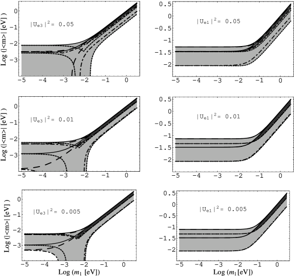
Figure 12: The dependence of $|\langle m\rangle|$ on $m_{1}$ in the case of the LMA-MSW solution of the solar neutrino problem [8] ($99.73\%$ C.L.), for the “normal” scheme in Fig. 7 (left panels), with $\Delta{m}^{2}_{\mathrm{sol}}=\Delta m_{21}^{2}$, and for the “inverted” scheme in Fig. 7 (right panels), with $\Delta{m}^{2}_{\mathrm{sol}}=\Delta m_{32}^{2}$. Figure taken from Ref. [148].

All previous conclusions are based on the assumption that the value of the effective Majorana mass $|\langle m\rangle|$ can be obtained from the measurement of the life-time of $(\beta\beta)_{0\nu}$-decay. There is, however, a serious theoretical problem in the determination of $|\langle m\rangle|$ from experimental data caused by the necessity to calculate the nuclear matrix elements.

In the framework of Majorana neutrino mixing, the total probability of $(\beta\beta)_{0\nu}$-decay has the general form (see Ref. [151])

$$\Gamma^{0\nu}(A,Z)=|\langle m\rangle|^{2}\,|M(A,Z)|^{2}\,G^{0\nu}(E_{0},Z)\,,$$ (5.26)

where $M(A,Z)$ is the nuclear matrix element and $G^{0\nu}(E_{0},Z)$ is a known phase-space factor ($E_{0}$ is the energy release). Thus, in order to determine $|\langle m\rangle|$ from the experimental data we need to know the nuclear matrix element $M(A,Z)$. This last quantity must be calculated.

There are at present large uncertainties in the calculations of the nuclear matrix elements of $(\beta\beta)_{0\nu}$-decay (see Refs. [152, 153, 154]). Two basic approaches to the calculation are used: quasi-particle random phase approximation and the nuclear shell model. Different calculations of the lifetime of the $(\beta\beta)_{0\nu}$-decay differ by about one order of magnitude. For example, for the lifetime of the $(\beta\beta)_{0\nu}$-decay of ${}^{76}\mathrm{Ge}$, assuming that $|\langle m\rangle|=5\times 10^{-2}\,\mathrm{eV}$, the range

$$6.8\times 10^{26}\,\mathrm{yr}\leq T^{0\nu}_{1/2}(^{76}\mathrm{Ge})\leq 70.8\times 10^{26}\,\mathrm{yr}$$ (5.27)

has been obtained (see Ref. [154]).

The problem of the calculation of the nuclear matrix elements of neutrinoless double-$\beta$ decay is a real theoretical challenge. It is obvious that without a solution of this problem the effective Majorana neutrino mass $|\langle m\rangle|$ cannot be determined from the experimental data with reliable accuracy (see the discussion in Ref. [155, 148]).

The authors of Ref. [156] proposed a method which allows to check the results of the calculations of the nuclear matrix elements of the $(\beta\beta)_{0\nu}$-decay of different nuclei by confronting them with experimental data. Let us take into account that

1. For small neutrino masses ($m_{i}\lesssim 10\,\mathrm{MeV}$) the nuclear matrix elements do not depend on the neutrino masses [151].

2. A sensitivity of a few $10^{-2}$ eV for $|\langle m\rangle|$ is planned to be reached in future experiments on the search for neutrinoless double-$\beta$ decay of different nuclei.

From Eq. (5.26) we have

$$R(A,Z/A^{\prime},Z^{\prime})\equiv\frac{T^{0\nu}_{1/2}(A,Z)}{T^{0\nu}_{1/2}(A^{\prime},Z^{\prime})}=\frac{|M(A^{\prime},Z^{\prime})|^{2}\,G^{0\nu}(E^{\prime}_{0},Z^{\prime})}{|M(A,Z)|^{2}\,G^{0\nu}(E_{0},Z)}\,.$$ (5.28)

Thus, if the neutrinoless double $\beta$ -decay of different nuclei is observed, the calculated ratios of the corresponding squared nuclear matrix elements can be confronted with the experimental values. Table 2 shows the ratios of the lifetimes of $(\beta\beta)_{0\nu}$-decay of several nuclei, calculated in six different models, using the values of the lifetimes given in Ref. [154]. As it is seen from Table 2, the calculated ratios vary within about one order of magnitude.

Lifetime Ratios	[157]	[158, 159]	[160]	[129]	[161]	[162, 163, 164]
$R(^{76}\mathrm{Ge}/^{130}\mathrm{Te})$	11.3	3	20	4.6	3.6	4.2
$R(^{76}\mathrm{Ge}/^{136}\mathrm{Xe})$		1.5	4.2	1.1	0.6	2
$R(^{76}\mathrm{Ge}/^{100}\mathrm{Mo})$			14	1.8	10.7	0.9

Table 2: The results of the calculation of the ratios of the lifetime of $(\beta\beta)_{0\nu}$-decay of several nuclei in six different models. The references to the corresponding papers are given in brackets.

As one can see from Table 2, the values of the ratio $R(^{76}\mathrm{Ge}/^{130}\mathrm{Te})$ calculated in Ref. [129] and Ref. [161] are, correspondingly, 4.6 and 3.6. It is clear that it will be difficult to distinguish models [129] and [161] through the observation of the neutrinoless double-$\beta$ decay of ${}^{76}\mathrm{Ge}$ and ${}^{130}\mathrm{Te}$. However, it will be possible to distinguish the corresponding models through the observation of the $(\beta\beta)_{0\nu}$-decay of ${}^{76}\mathrm{Ge}$ and ${}^{100}\mathrm{Mo}$ (the values of the corresponding ratio are 1.8 and 10.7, respectively). This example illustrates the importance of the investigation of $(\beta\beta)_{0\nu}$-decay of more than two nuclei.

The nuclear part of the matrix element of $(\beta\beta)_{0\nu}$-decay is determined by the matrix element of the $T$-product of two hadronic charged currents connected by the propagator of a massless boson. This matrix element cannot be connected with the matrix element of any observable process. The method proposed in Ref. [156] is based only on the smallness of neutrino masses and on the factorization of the neutrino and nuclear parts of the matrix element of $(\beta\beta)_{0\nu}$-decay. It requires observation of the $(\beta\beta)_{0\nu}$-decay of different nuclei.

Let us notice that, if the ratio in Eq. (5.28), calculated in some model, is in agreement with the experimental data, it could only mean that the model is correct up to a possible factor, which does not depend on $A$ and $Z$ (and drops out from the ratio (5.28)). Such factor was found and calculated in Ref.[163], where in addition to the usual axial and vector terms in the nucleon matrix element pseudoscalar and weak magnetic form factors were taken into account. It was shown that in the case of light Majorana neutrinos these additional terms lead to a universal reduction of the nuclear matrix elements of $(\beta\beta)_{0\,\nu}$-decay by about 30 %. This reduction, which practically does not depend on the type of nucleus, causes a raise of the value of the effective Majorana mass $|\langle m\rangle|$ that could be obtained from the results of future experiments.

6 Cosmology

Perhaps the best example of the fruitful cross-fertilization of high energy physics and cosmology is the momentous constraint by Big-Bang Nucleosynthesis (BBN) [43] on the number of light neutrino species. Indeed, the number of effective light degrees of freedom affects the expansion rate of the Universe; the larger this number, the larger is the expansion rate and hence the higher the freeze out temperature of the weak interactions that inter-convert neutrons and protons. Thus, the neutron to proton ratio is correspondingly higher and so is the primordial helium yield. These events took place when the temperature of the universe was of the order of 1 MeV and therefore it is clear that neutrino masses at the 1 eV scale or less play no significant role in primordial light element formation. As a consequence, no relevant information on the absolute value of light neutrino masses from those early epochs of the history of the universe can be gained. This does not mean, however, that cosmology cannot supply interesting information on the neutrino mass issue. Fortunately, we can learn about neutrino mass from various cosmological and astrophysical instances as different as the Cosmic Microwave Background radiation (CMB), the power spectrum in large scale structure (LSS) surveys, and Lyman $\alpha$ (Ly$\alpha$) forest studies. We will address these issues in what follows (see also the reviews in Refs. [26, 37, 38, 39, 40, 44]).

6.1 The Gerstein-Zeldovich limit on neutrino masses

Before entering the issues mentioned explicitly above, let us present the “classical” cosmological bound on the sum of the masses of all neutrino species derived by Gerstein and Zeldovich [46, 47]. Stable light neutrinos (i.e. relativistic at neutrino decoupling) are present in the Universe today with an abundance of about $100$ neutrinos and antineutrinos per $\mathrm{cm}^{3}$. If they carry mass and this mass is much larger than the present CMB temperature (i.e. $m_{\nu}\gg kT_{\mathrm{CMB}}\sim 3\times 10^{-4}\,\mathrm{eV}$, with $T_{\mathrm{CMB}}\simeq 3\,\mathrm{K}$), they contribute to the known mass density $\Omega_{m}$ (relative to the critical density $\rho_{c}=3H_{0}^{2}/8\pi G_{N}$, where $H_{0}$ is the Hubble constant and $G_{N}$ is the Newton gravitational constant) associated to nonrelativistic matter (mainly dark). The energy density associated to neutrino mass can be thus be written as

$$\Omega_{\nu}h^{2}=\sum_{i}\frac{m_{i}}{93\,\mathrm{eV}}\,,$$ (6.1)

where, as usual, the Hubble constant is parameterized as $H_{0}=100h$ km/s/Mpc.

Since observationally $\Omega_{m}h^{2}\approx 0.15$ and $\Omega_{\nu}<\Omega_{m}$, it follows that $\sum_{i}m_{i}<14$ eV. For mass degenerated neutrinos this bound implies that $m_{i}<5$ eV for each species.

6.2 Microwave Background Anisotropies

The background radiation first detected by Penzias and Wilson in the late fifties follows an almost perfect black-body spectrum at the temperature $T_{0}=2.728\pm 0.002\,\mathrm{K}$. This radiation is extremely isotropic so that this temperature on the sky is direction independent to a precision of $10^{-5}$, once the Doppler effect due to the peculiar velocity of the Solar System is removed. However the Universe is highly inhomogeneous today and this means that it should have been sufficiently inhomogeneous in the past in order that structure could grow via gravitational instability. Therefore, density inhomogeneities should give rise to temperature inhomogeneities in the sky [166]. For many years such temperature fluctuations in the cosmic background radiation have been searched for until they have been finally established at the aforementioned minute $10^{-5}$ level by COBE [167]. It is customary to expand the temperature fluctuations ${\Delta T/T_{0}}$ in spherical harmonics

$$\frac{\Delta T}{T_{0}}=\sum_{l\geq 2}a_{lm}Y_{lm}(\theta,\varphi)\,.$$ (6.2)

The coefficients $a_{lm}$ are random variables with zero mean $\langle a_{lm}\rangle=0$ and variance $\langle a_{lm}^{*}a_{l^{\prime}m^{\prime}}\rangle=C_{l}\delta_{ll^{\prime}}\delta_{mm^{\prime}}$ as required by the statistical isotropy of temperature fluctuations. The $C_{l}$’s form the angular power spectrum and this angular power spectrum is conventionally shown when presenting CMB results (see Fig. 13). The CMB photons that we now record were last scattered at recombination when the universe was about $300,000$ yr old and the redshift was $z\sim 1100$. So, what we get from the temperature fluctuation spectrum is essentially a snapshot of the density inhomogeneities at recombination. It is not quite a $bonafide$ picture of the anisotropies at that time because in their way to us the cosmic photons should have experienced gravitational redshift by changing gravitational potentials, the so-called Integrated Sachs-Wolfe effect (ISW) [169], and eventually, rescattering by ionized gas in interposed clusters of galaxies (Sunyaev-Zeldovich effect [170]). The primary causes of temperature anisotropy, those present at recombination, are threefold. There is an intrinsic source associated to the fact that denser spots are hotter and hence photons emerging from those denser regions are bluer. But also, photons in denser regions will be redshifted as they climb out of their potential wells (Sachs-Wolfe effect (SW) [169]). These are competing effects and it depends on the scale under scrutiny that one or the other dominates. And finally, the third source of temperature anisotropy generation is associated to Doppler shifts arising from the peculiar motion of matter in underdense regions being attracted towards overdense regions and from which photons are last scattered. We collect the three primary sources in the formula:

$$\frac{\Delta T}{T_{0}}=\left(\frac{\Delta T}{T}\right)_{intr}+\phi-{\hat{n}}\cdot\vec{v}\,,$$ (6.3)

where $\phi$ is the gravitational potential well, $\vec{v}$ is the peculiar velocity, and $\hat{n}$ is a unit vector pointing in the direction $\theta,\varphi$.

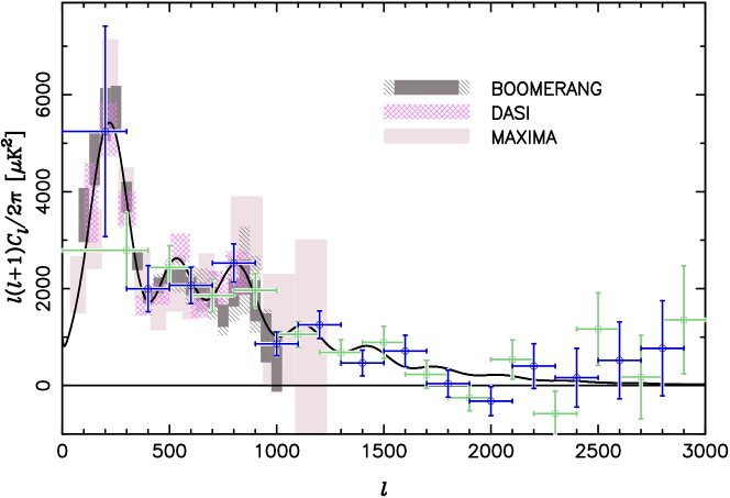
Figure 13: A recent plot of the anisotropy spectrum taken from Ref. [168]. It shows BOOMERANG, DASI, MAXIMA, and CBI data (squares and circles). See Ref. [168] and references therein for details.

To connect the observational CMB anisotropy data with the underlying cosmological model and thus have a handle on the different cosmological parameters one has to work out the different pieces in the previous equation in terms of the matter density inhomogeneities and peculiar velocity of the photon-baryon fluid at recombination. These density fluctuations and peculiar velocity, in turn, have to be obtained from the general relativistic equations (and/or their newtonian counterparts, when appropriate) to take into account their time evolution from given initial (end of inflation) conditions (adiabatic) up to recombination. Since density perturbations are supposedly small over the whole period of interest (up to recombination), one uses linear perturbation theory to deal with the problem which then becomes easy to solve. Indeed, a main feature of the linearized theory is that by Fourier transforming from $r$ $space$ into $k$ $space$, the different $k$ $modes$ become mutually independent and therefore the corresponding spatial scales evolve independently during the linear era of structure formation. Because each $k$ $mode$ corresponds to a different spatial size $\lambda$ ($\lambda={2\pi/k}$), a given mode enters the horizon at a given epoch. But crossing the Hubble radius is physically relevant since before crossing a scale evolves solely under the rule of gravity and only after horizon crossing are also causal effects operative. A sub-horizon sized fluctuation, therefore, experiences both the gravitational pull and the pressure gradients of the photon-baryon fluid. Too much gravity pull cannot be counteracted by fluid pressure, hence there is a critical size for a perturbation to stand gravity. Beyond that size (so called Jeans size), collapse is unimpeded but below the Jeans size collapse can be halted. This Jeans scale is set by the sound speed in the primeval plasma because it determines the distance over which a mechanical response of pressure forces can propagate over a gravitational free-fall time and thus restore hydrodynamical equilibrium in the fluid. For those under-sized perturbations, acoustic oscillations set in: compression is followed by rarefaction and back to compression and so forth because the in-falling fluid bounces off every time the pressure of the fluid rises to the point where it can halt gravitational in-fall and reverse the process from contraction to expansion. Since before recombination the pressure of the baryon-photon plasma is dominated by photon pressure, the sound velocity is roughly $c_{s}\sim c/\sqrt{3}$, close to the speed of light. So, during the pre-recombination stages, the sound horizon approximately matches the Hubble radius and thus scales entering the horizon before recombination undergo acoustic oscillations from that moment onwards. Later, when recombination takes place and photons are freed from the baryons to which they were previously tightly bound, the different modes (scales) are caught at different phases of their oscillation with correspondingly different amplitudes of their density perturbations. These compression and rarefaction phases translate into peaks in the temperature power spectrum that one observes. Odd peaks correspond to compression maxima and even peaks correspond to compression minima (rarefaction peaks). The first peak is associated to the scale that enters the horizon at recombination and is thus caught in its first oscillation height. The second peak corresponds to a scale that has already gone through a complete oscillation cycle at recombination, etc. Because the smaller the scale the sooner it entered the horizon, and therefore will have got time for a longer period of oscillations before photon decoupling, the corresponding peaks in the power spectrum are progressively attenuated as compared to the first compression maximum. The main source of damping, which is called Silk damping [171], is due to the fact that photons in the baryon-photon fluid have a mean free path governed by the Thomson cross section (photons are coupled to the electrons via Thomson scattering and electrons in turn are tightly bound to protons via Coulomb interactions) and so photons tend to leak out from overdense regions to less dense regions whenever the photon mean free path (which depends on the ionization history before recombination and on the baryon content) exceeds the scale of the density fluctuation. In addition to this there is also a limit to the pattern of peaks supplied by the finite width of the last scattering surface. Since recombination is not instantaneous but takes a finite amount of time, observations of the cosmic background temperature are actually an average over temperatures of photons that reach us from a shell whose thickness is about one tenth the Hubble distance at recombination [172]. Hence, scales that are of this order of magnitude or less are completely washed out by the temperature averaging process. For a flat universe this limit corresponds to angular scales of about $0.1$ deg or to multipoles larger than about $l\sim 2000$. We are prepared now to discuss what can be learned from the peak structure of the power spectrum as far as general cosmological parameters is concerned (including the neutrino energy content, which is our main concern here).

The characteristics of the spectrum of CMB anisotropies and of its peaks ( i.e. their positions, heights, and shapes) depend on the adopted cosmological model for the initial anisotropies and on all the parameters that govern the evolution of the acoustic oscillations before recombination and on the hindrances encountered by photons in their paths from recombination onwards. Clearly, not all parameters affect to the same extent the different aspects of the power spectrum pattern. Let us remind here of the main influences on the power spectrum features and let us leave for later the neutrino mass related issues:

1. At large angular scales (i.e., large compared to the horizon scale at recombination), the SW effect dominates the anisotropies. Those are the scales that, at recombination, have had no microphysics processing yet and reflect directly the character and strength of the primordial inhomogeneities. Therefore, one can read from the observed spectrum at large angular scales (small $l$’s) the general cosmological paradigm about the origin of inhomogeneities. For instance, a flat spectrum (as it is indeed the case) in this low $l$ regime suggests an adiabatic scale-invariant inflationary-like model of primordial anisotropies.

2. When a physical feature on the last scattering surface at recombination is projected on the sky today, the projection depends on the distance to last scattering and on the curvature of space. The distance is fixed by $t_{rec}$ and hence depends mainly on the Hubble constant and total energy density $\Omega$. Curvature affects the projection because it is an obvious geometric fact of curved spaces that objects seem to be smaller (larger) in an open (closed) Universe then they would in a flat Universe. Thus the angle $\theta$ subtended by a given structure on the sky (its angular size) depends on curvature. Recall that the first peak corresponds to the scale that enters the horizon at recombination. So, its location in $l$ ($l\sim\theta^{-1}$) tells us about the curvature of the Universe. For a zero curvature Universe the position of the first peak should be at $l_{1}\sim 200$, which is actually the case of the observed spectrum (see Fig. 13).

3. Baryons contribute inertia to the oscillating photon-baryon plasma in the dark matter potential wells and as a consequence the bigger the baryon content is the larger the amplitudes of the acoustic vibrations are (i.e., the peaks are higher). Furthermore, compression peaks (odd peaks) are enhanced relatively to rarefaction peaks (even peaks) as a result of baryon drag.

Unfortunately there is a substantial amount of degeneracy among the cosmological parameters [173] that allow for a multiplicity of different parameter choices giving an equally acceptable spectrum. So it is very desirable to use alternative measurements as complementary tools for determining cosmological parameters and thus help break degeneracies. For instance, for a flat Universe ($\Omega\sim 1$, as it is indeed the case; see point 2 above) the position of the first peak is almost independent of the relative weight of matter (baryonic plus dark) and dark energy (cosmological constant) in $\Omega$.

Nonzero mass neutrinos affect the CMB anisotropy spectrum to a much lesser extent than the previously stated effects [174]. Their influence is twofold: the position of the peaks is slightly modified and also their amplitudes are enhanced. Although the position of the first peak is mostly dictated by curvature, the peaks and the troughs move slightly to lower $l^{\prime}s$ (to the left in Fig. 13) due to massive neutrinos. This effect can be traced back to the fact that neutrinos being massive, they start being ultrarelativistic until their freeze out and beyond and only later in the history of the Universe the neutrinos become nonrelativistic. Compared to the massless neutrino case where neutrinos are always relativistic degrees of freedom, in the case under discussion, the expansion rate is slightly modified since the competition between radiation domination and matter domination is altered. While the propagation of sound in the photon-baryon fluid depends only on the baryon density and hence neutrino mass is not relevant here, the sound horizon at decoupling is modified simply because decoupling is slightly delayed due to the change in expansion rate. If the sound horizon is larger, so it is the scale that enters the horizon at last scattering. Therefore, larger angular scales corresponding to lower $l^{\prime}s$, the pattern of acoustic peaks is shifted to the left. The neutrino mass, on the other hand, has a larger impact on the power spectrum than the shifting just mentioned; it leads to an enhancement of the peaks. The origin of the effect is related to the time variation of the gravitational potentials. In a radiation dominated Universe potentials change with time whereas in a matter dominated Universe gravitational potentials are constant. Since a Universe with massive neutrinos implies that relativistic matter turns into non-relativistic matter during relevant periods of its evolution, the acoustic oscillations of the baryon-photon plasma are being forced by time decaying potentials that differ from those associated to a Universe with massless neutrinos only. As a result the acoustic oscillations (mainly for $l\geq 300$) get an extra boost in amplitude at last scattering (parametric resonance). There is also a smaller effect associated to varying potentials after last scattering that introduces a relative difference between models with/out massive neutrinos (affecting the ISW contribution to anisotropies) which is operative at smaller $l^{\prime}s$.

6.3 Galaxy Redshift Surveys

In the previous section we gave a brief and general description of the physics of the CMB angular power spectrum and noted that the direct influence upon it of neutrino mass is only marginal. Yet, the CMB power spectrum data is important in the determination of neutrino mass because it can be used in combination with other astrophysical sources – where the neutrino mass plays a more relevant role – to help reduce the number of uncertainties in the various cosmological parameters. One of these sources is large scale structure. Neutrino mass affects large scale structure formation and its effect can be studied via observation of the distribution of galaxies. Since the distribution of galaxies should trace the matter density of the Universe (related to each other via a bias factor), large samples of galaxy redshifts in surveys such as the 2 degree Field Galaxy Redshift Survey (2dFGRS) [175] provide a tool to study the power spectrum of matter fluctuations with very small random errors.

Recall that in linear theory what one is dealing with is the Fourier transformed density perturbations $\delta_{k}$. The initial conditions for $\delta_{k}$ are set to reproduce a property of inflation (and consistent with observations), i.e. a flat or Harrison-Zeldovich spectrum is assumed. This implies that the power spectrum behaves as $P(k)=\langle\delta_{k}^{2}\rangle\sim k^{n}$ with $n\simeq 1$. This initial spectrum has to be evolved from the very high initial redshifts to the redshifts relevant for structure formation surveys (the median redshift of 2dFGRS is $\sim 0.1$ [175]). This processing is dictated by the continuity, Euler and Boltzmann equations that govern the physics of the perturbations of the cosmic fluid. To be specific, what concerns us here is the effect of massive neutrinos on the evolution of perturbations, i.e on the power spectrum $P(k)$. Once decoupled very early in the history of the Universe (at $T\sim 1$ MeV) neutrinos free-stream at almost the speed of light. This is so until after their momenta become on the order of their mass and less and hence they enter a non-relativistic regime. During their relativistic life-span they outflow from regions smaller than the horizon so that these regions are being depleted and hence energy density perturbations at those scales are effectively erased. This phenomenon comes to an end when neutrinos cease to free-stream as they become non-relativistic and can cluster with the cold components of dark matter for all scales that are larger than the Hubble radius at the time the neutrinos become non-relativistic. This limiting scale is given by the formula [176]:

$$k_{nr}\simeq 0.03(m_{\nu}/1\,\mathrm{eV})^{1/2}\Omega_{m}^{1/2}h\mathrm{Mpc}^{-1}\,.$$ (6.4)

For all scales smaller than this (i.e. for $k\geq k_{nr}$) the growth of perturbations is suppressed. So neutrino mass influences the power spectrum of cosmological structure at small scales. The loss of power on small scales can be approximated by [176]

$$\frac{\Delta P}{P}\approx-8\frac{\Omega_{\nu}}{\Omega_{m}}\,.$$ (6.5)

This equation gives us a handle for extracting the bounds on neutrino mass from the large samples of data in present and upcoming galaxy distribution surveys (see Fig. 14). The analysis of the data has to be restricted to a band of scales for which the data are precise enough and for which linear perturbation theory holds. On the large scales side accuracy is volume limited and on the small scales side linear theory is jeopardized. The 2dFGRS data, for instance, are robust on scales $0.02<k<0.15$ $h$ $\mathrm{Mpc}^{-1}$.

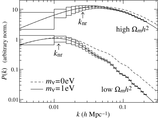
Figure 14: Effect of a 1 eV neutrino on $P(k)$ as found by the authors of Ref. [176].

6.4 Lyman $\alpha$ forests

The last piece of information relevant to the neutrino mass issue that we want to discuss is the Ly$\alpha$ forest [177] measurements of the power spectrum of mass fluctuations. Quasars are of help in cosmology because for one thing they rank among the oldest detected objects in the Universe and hence provide crucial hints for structure formation studies. Furthermore, quasar spectra are a means for studying the intergalactic medium. Atomic hydrogen in the gas clouds in the vicinity of the quasar makes $2p\to 1s$ Ly$\alpha$ transitions that are seen redshifted today by a factor $1+z_{quasar}$. But what is most important here is that quasar spectra show a series of absorption lines associated to intervening clouds that photons encounter in the way from the quasar to us. Indeed, the spectrum displays a “forest” of Ly$\alpha$ absorption lines to the left of the Ly$\alpha$ emission line of the quasar, i.e. blueshifted relatively to the emitter, that correspond to the resonant absorption of those photons – with wavelengths $\lambda$ stretched by cosmic expansion in the proportion $(1+z_{quasar})/(1+z_{cloud})$ – that exactly match the Ly$\alpha$ transition. The forest of absorption lines in the quasar spectrum refers therefore to a sequence of clouds at various redshifts along our line-of-sight towards the quasar that absorb radiation from the quasar at specific wavelengths given by the redshift of each cloud relative to the quasar’s own redshift. The distribution of such clouds thus can provide astronomers with important clues about structure formation. In particular, since light neutrinos do not cluster on small scales as was explained in the previous section, the measurement of cluster formation on small scales extracted from Ly$\alpha$ forest observations can lead to definite predictions for neutrino mass in the eV range.

6.5 Neutrino mass bounds

Now that we discussed the different cosmological and astrophysical sources of information on neutrino mass, we can summarize the constraints on neutrino masses that follow from these sources [178].

Absolute neutrino masses cannot be measured in neutrino oscillation experiments. Only mass-squared differences have been established so far. If the three neutrino mass spectrum is hierarchical then $m_{1}\simeq 0$, $m_{2}\simeq\sqrt{\Delta{m}^{2}_{\mathrm{sol}}}$, and $m_{3}\simeq\sqrt{\Delta{m}^{2}_{\mathrm{atm}}}$. Should, on the other hand, the mass hierarchy be inverted, then $m_{1}\simeq 0$, $m_{2}\simeq\sqrt{\Delta{m}^{2}_{\mathrm{atm}}}$, and $m_{3}\simeq\sqrt{\Delta{m}^{2}_{\mathrm{atm}}}$. The third possibility is mass degeneracy, i.e. $m_{1}\simeq m_{2}\simeq m_{3}$. In this case the three masses would be much bigger than $\sqrt{\Delta{m}^{2}_{\mathrm{atm}}}$ and any hint as to their absolute mass scale is lost in neutrino oscillations. In this instance astrophysical/cosmological tests come to the rescue.

The Ly$\alpha$ forest seen in quasar spectra, as mentioned in the previous section, can be used to study mass distribution fluctuations. There is a well-understood theory of Ly$\alpha$ forest formation embodied in the standard cosmology which establishes a rather simple local connection between the absorbed flux in a quasar spectrum and the underlying matter density. From this relationship, the power spectrum $P(k)$ can be extracted, at least over a limited range of scales [179].

Indeed, in the usual cosmological scenario where structure formation proceeds via gravitational instabilities, the behavior of gas plus a background of UV ionizing radiation leads naturally to quasar absorption effects. The physics of the gas is driven by the competition of two phenomena, namely adiabatic cooling due to Hubble flow, and heating by the photo-ionizing UV background. Hydrodynamic simulations show that the Ly$\alpha$ forest arises in gas of moderate overdensity [180]. This density field can be then locally related to the Ly$\alpha$ optical depth [181], and consequently to the observed transmitted flux in a quasar spectrum.

Light neutrinos delay the growth of perturbations at small scales and therefore a constraint on their mass is made possible through the recovery of the power spectrum $P(k)$ from an observational measurement of the Ly$\alpha$ forest. The authors of Ref. [182] used the measurement in [183] to restrict light neutrino masses. Their general strategy consisted of two steps. In a first step they tested hydrodynamic Ly$\alpha$ forest simulations in the context of a cosmological model with non-zero mass neutrinos. Specifically, what they wanted to check is their ability to recover, in a given cosmological setting, the power spectrum $P(k)$ from a hydrodynamic simulation of the forest. The method had been previously used in models that do not include “hot particles”, i.e. models without massive neutrinos. The assumed underlying cosmological scenario is an adiabatic, cold dark matter dominated Universe with gaussian initial fluctuations. Such models contain six free parameters, namely: the matter density $\Omega_{m}$, the Hubble parameter $h$, the baryon density $\Omega_{b}$, the neutrino density $\Omega_{\nu}$, and the amplitude and tilt of the initial power spectrum of density perturbations $Ak^{n}$. A flat spatial geometry is also assumed throughout as the CMB anisotropy and supernova measurements seem to corroborate. The particular model used in the tests has $\Omega_{m}=1$, $h=0.5$, $\Omega_{b}=0.075$, and $\Omega_{\nu}=0.2$. The hydrodynamic simulation [184] allows then to follow the evolution of structure in this model and to know the physical condition and distribution of the gas at $z=2.5$ (i.e. at the redshift of the actual measurements). From this, they generated artificial Ly$\alpha$ spectra for 1200 random lines of sight through the simulation volume. The recovery procedure was applied then to these spectra to see if the recovered $P(k)$ agrees with the linear theory prediction of the model under scrutiny. The authors obtained a fair amount of consistency over the whole observational band of scales and concluded from their simulation tests that their recovered $P(k)$ was systematically too low in amplitude and had a somewhat flatter slope than the linear theory prediction (however, the authors point out that correcting for this underestimation would lead only to tighter neutrino mass limits). Having proved that the method works for a specific model, it was assumed that it would also work for all cosmological models with massive neutrinos available in parameter space. The final step involves using the observational results on the Ly$\alpha$ forest to explore the six dimensional parameter space and place an upper limit on the neutrino mass.

The loss of power in the Ly$\alpha$ forest induced by a neutrino mass is given by equation (6.5) but other parameters could produce similar power suppression effects. To avoid as much as possible undesired degeneracies, the authors use additional cosmological constraints. They use the Hubble constant measurement [185], the COBE detection of large scale anisotropies [186], the present abundance of galaxy clusters [187], galaxy surveys [188], nucleosynthesis limits on baryon abundance [189], and the age of the oldest globular clusters to set a lower limit to the age of the Universe [190]. In their analysis the authors reject every model that violates the 95% C.L. on any of the aforementioned constraints. With such reduced parameter space, the analytic approximations of [191] were used to find the model that maximizes $\Omega_{\nu}$ as a function of $\Omega_{m}$. The result is

$$\sum_{i}m_{i}<5.5\,\mathrm{eV}\qquad(95\%\,\mathrm{C.L.})\,,$$ (6.6)

independently of the value of $\Omega_{m}$.

If $\Omega_{m}$ is restricted to lie in the range $0.2-0.5$ as favored by observation, then the authors parameterize their bounds as

$$m_{\nu}\leq 2.4\left(\frac{\Omega_{m}}{0.17}-1\right)\mathrm{eV}\qquad(95\%\,\mathrm{C.L.})\,.$$ (6.7)

There have been several analysis that put constraints on neutrino masses from LSS redshift surveys. The most recent ones make use of the 2dF galaxy survey [175]. The 2dFGRS is a sample of over 220,000 galaxy redshifts that permits the measurement of large-scale structure statistics with very small random errors. Ref. [192] computes the matter power spectrum from linear theory for a multiplicity of cosmological models described in terms of the components: baryons, cold dark matter, cosmological constant, and of course hot dark matter (i.e. neutrinos with non-zero mass). The calculated matter power spectrum and the measured galaxy power spectrum can be put in correspondence through a bias parameter, i.e. $b^{2}\equiv P_{g}(k)/P_{m}(k)$, where $P_{g}(k)$ is the measured galaxy distribution power spectrum and $P_{m}(k)$ is the matter power spectrum. Although $b$ is in principle scale dependent, there are good reasons to believe that $b$ is a constant on the scales considered in the analysis [193]. The authors of this study absorbed this constant in the amplitude $A$ of the power spectrum of density fluctuations taken as a free parameter. There is a vast parameter space available for the analysis, and again it helps to take other cosmological inputs into consideration. In this way the implications for neutrino mass will be less uncertain.

From primordial nucleosynthesis one has the constraint $\Omega_{b}h^{2}=0.020\pm 0.002$ on the density of baryons [194]. The Hubble parameter $h$ as measured by the Hubble Space Telescope (HST) key project [195] is $h=0.70\pm 0.07$. Another prior is the total matter density $\Omega_{m}$. As stated before when we discussed the peak structure of the CMB anisotropy spectrum, there is strong evidence for a spatially flat Universe [196]. This means $\Omega_{m}+\Omega_{\Lambda}=1$. This last relation, used together with the results from surveys of high redshift Type Ia supernovae (SNIa) [197, 198], leads to the constraint $\Omega_{m}=0.28\pm 0.14$. On the other hand, independent studies give a wider spread of values. For instance, mass-to-light ratio studies of galaxy clusters render typically lower values for $\Omega_{m}$ ($\sim 0.15$) [199] whereas cluster abundance studies deliver $\Omega_{m}\approx 0.3-0.9$ [200]. Given these facts that make $\Omega_{m}$ the most poorly known parameter, the authors of the present analysis employed two kinds of priors on $\Omega_{m}$. One was a Gaussian at $\Omega_{m}=0.28$ and standard deviation 0.14 as required by supernova and CMB results and the other was a uniform prior in the range $0.1<\Omega_{m}<0.5$. The latter upper limit ($\Omega_{m}<0.5)$ is dictated by the values of $h$ used which would imply, for $\Omega_{m}>0.5$, an age of the Universe shorter than 12 Gyr. Although the value $n=1$ for the spectral index is the usual theoretical choice, $n=1\pm 0.1$ is also acceptable and consistent with the CMB data. Therefore, the authors of Reference [192] considered the cases $n=0.9$ and $n=1.1$ and they ran a grid of models with $n$ as an added parameter restricted to the values $n=1\pm 0.1$ (Gaussian prior).

Their results can be summarized as

$$\sum_{i}m_{i}<1.8\,\mathrm{eV}\qquad(95\%\,\mathrm{C.L.})\,,$$ (6.8)

for $\Omega_{m}h^{2}=0.15$ (for the central values of $\Omega_{m}$ and $h=0.7$; actually, almost identical results follow from the two distinct priors on $\Omega_{m}$) and spectral index $n=1$. If this latter condition is relaxed to $n=1.0\pm 0.1$, then a somewhat looser bound is obtained:

$$\sum_{i}m_{i}<2.2\,\mathrm{eV}\qquad(95\%\,\mathrm{C.L.})\,.$$ (6.9)

Other groups [201, 202] obtain results from LSS that are fully compatible with the previous upper bounds on neutrino masses. Hannestad in Ref. [201] performs a full numerical likelihood analysis in a cosmological parameter space with the following free parameters (other than $\Omega_{\nu}$): $\Omega_{m}$, $\Omega_{b}$, $h$, $n$, the normalization of the CMB power spectrum $Q$ and the optical depth to reionization $\tau$. Also, he restricts the study to flat models, i.e. with zero curvature. This is by no means a drawback since there is little degeneracy between neutrino mass and curvature. The analysis is presented in three stages, depending on the data sets used and on the corresponding priors for the cosmological parameters other than neutrino mass. In the first stage LSS [203] data and CMB [167, 204] data alone are used. The resulting bound is, in this instance,

$$\sum_{i}m_{i}<2.96\,\mathrm{eV}\qquad(95\%\,\mathrm{C.L.})\,.$$ (6.10)

The second stage incorporates Big-Bang Nucleosynthesis [205] and Hubble Space Telescope [195] data in the analysis (in addition to the previous data sets). This entails the Big-Bang Nucleosynthesis prior on the baryon density $\Omega_{b}h^{2}=0.020\pm 0.002$ and the HST key project prior on the Hubble parameter already given above. This leads to a slight improvement of the bound:

$$\sum_{i}m_{i}<2.65\,\mathrm{eV}\qquad(95\%\,\mathrm{C.L.})\,.$$ (6.11)

Finally, including the data from high redshift Type Ia supernova surveys [197] Hannestad obtains:

$$\sum_{i}m_{i}<2.47\,\mathrm{eV}\qquad(95\%\,\mathrm{C.L.})\,.$$ (6.12)

Here, the result $\Omega_{m}=0.28\pm 0.14$ (valid for a flat Universe) has been used. (In all three cases above, $Q$ and $b$ are allowed to vary freely, $\tau=0-1$ and $n=0.66-1.34$. In the first and second stages, $\Omega_{m}=0.1-1$. In stage one, $\Omega_{b}h^{2}=0.008-0.040$ and $h=0.4-1.0$.)

Lewis and Bridle [202] use the sets of observational data on the CMB, LSS, BBN, HST and SNIa, that we are already familiar with, to explore the consequences of a non-zero neutrino mass under somewhat less restricted assumptions than in the analysis just discussed [201]. In particular, they consider nine parameter model universes that include parameters that account for a “quintessential” equation of state and tensor contributions to the power spectrum (allowed in inflationary models). Perhaps the most distinctive feature of the present analysis is the use of powerful Markov Chain Monte-Carlo techniques to perform a fast and efficient exploration of a high dimensional cosmological parameter space. As a result of these methods, reference [202] reports

$$\sum_{i}m_{i}<1.5\,\mathrm{eV}\qquad(95\%\,\mathrm{C.L.})\,.$$ (6.13)

For the sake of completeness we should include here the result obtained in Ref. [206], namely (for the case of mass degeneracy):

$$m_{i}<0.9\,\mathrm{eV}$$ (6.14)

for $h\leq 0.8$, $\Omega_{m}\leq 0.4$, and an age for the Universe in excess of $11.5$ Gyr. However, the approach of this work is different from what has been discussed here so far. It is based on the matching condition for the cosmic mass density fluctuation power at the COBE scale and the matter clustering power at the cluster scale. As the authors put it, the advantage of using the cluster abundance information is that it refers to the mass function which is not affected by any biasing uncertainties (i.e. to what extent galaxies trace the mass distribution).

To summarize all these findings, we can say that the bound

$$\sum_{i}m_{i}\lesssim 3\,\mathrm{eV}$$ (6.15)

should be a reliable upper limit on the sum of neutrino masses which implies that (again, for three almost degenerate neutrinos)

$$m_{i}\lesssim 1\,\mathrm{eV}$$ (6.16)

for each of the three masses.

As to future prospects, MAP/PLANCK CMB data in conjunction with high precision galaxy surveys such as the Sloan Digital Sky Survey [207] could render [176]

$$\sum_{i}m_{i}<0.3\,\mathrm{eV}$$ (6.17)

or [208]

$$\sum_{i}m_{i}<0.12\,\mathrm{eV}$$ (6.18)

at 95% C.L., or even go down to an ultimate sensitivity of about $0.04$ eV when weak lensing of galaxies by large scale structure is also taken into account [209].

To conclude, perhaps we should mention here a result [210] that has an extra theoretical input, namely leptogenesis as the origin of matter-antimatter asymmetry. In such scenario, neutrinos are Majorana particles, and for the whole picture to work, such neutrinos should weigh less than $0.2$ eV.

7 Cosmic Rays

Since the sixties [49, 50] it is well-known that the universe is opaque to protons (and other nuclei) on cosmological distances. An ultra high energy (UHE) proton with energy $E$ exceeding the Greisen-Zatsepin-Kuzmin (GZK) energy

$$E_{\mathrm{GZK}}\sim 5\times 10^{19}\ \mathrm{eV}$$ (7.1)

interacts with the photons of the cosmic background producing pions through the $\Delta^{*}$ resonance, $p+\gamma_{CB}\rightarrow\Delta^{*}\rightarrow N\pi$. In this way, the initial proton energy is degraded with an attenuation length of about 50 Mpc [49, 50]. The UHE photons have even shorter absorption lengths ($\sim 10\,\mathrm{Mpc}$ for $E\sim 10^{20}$ eV [211]) due to their interactions with cosmic background photons [212]. Since plausible astrophysical sources for UHE particles (like AGNs) are located at distances larger than 50-100 Mpc, one expects the so-called GZK cutoff in the cosmic ray flux at the energy given by (7.1).

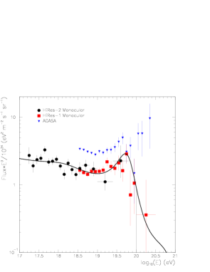
Figure 15: UHE Cosmic Ray Flux times E³. Results from the HiRes-I and HiRes-II detectors, and the AGASA experiment are shown. Also shown (solid curve) is a fit to the data assuming a model with two sources of cosmic rays, galactic and extragalactic, which includes the GZK cutoff. Figure taken from Ref. [222].

However, in the cosmic ray data [213, 214, 215, 216, 217, 218, 219, 220, 221, 222], there are about twenty cosmic ray events with energies just above the GZK energy (see Fig. 15). Yet, the whole observational status in the UHE regime is controversial. While the HiRes collaboration claim [222] that they see the expected event reduction, a recent reevaluation of AGASA data seems to confirm the violation of the GZK cutoff [221]. Indeed, some apparent inconsistencies among data have been pointed out [223]. The observational status is not settled, but it is clear that if the GZK violation is confirmed, the origin of the super-GZK particles constitutes one of the most pressing puzzles in modern high-energy astrophysics (for a recent review, see Ref. [224]).

Several hypothetical explanations have been put forward to account for this phenomenon. For example, there are scenarios where the UHE cosmic rays are decay products of exotic super-massive particles or relic topological defects. Also, a way to solve the problem might be to postulate a violation of Lorentz symmetry, or introduce new particles or/and new interactions (for a recent review, see Ref. [224]). We are concerned here with a possible explanation that is based on the so-called $Z$-bursts [51, 52]. If the GZK cutoff is violated and the Z-burst mechanism is indeed the solution to the GZK puzzle, it may be used to determine the absolute value of neutrino masses and, in fact, it would be an indirect proof of the existence of the relic cosmic background neutrinos.

The main hypothesis of the Z-burst explanation of the GZK puzzle is the existence of a very high flux of UHE neutrinos. And the main criticism to it is that standard astrophysical objects cannot produce such fluxes. Thus, the Z-burst hypothesis requires new sources producing UHE neutrinos copiously. (If the flux is so large, it may be measured by the next generation of neutrino telescopes; see Ref. [225].) However, compared to the other models quoted before, the Z-burst scenario does not need new physics beyond the Standard Model of particle physics with neutrino masses.

The crucial observation is that neutrinos, contrary to protons and photons, propagate over cosmological distances with negligible opacity. The most important interaction they have is with cosmic background neutrinos. Although this represents a extremely small opacity it might be enough to generate the UHE cosmic rays.

Cosmic background neutrinos are the relics of neutrino decoupling in the early Universe, that happened when the Universe was about 1 second old and had a temperature of about 1 MeV. Their number density today can be calculated easily in terms of the observed number density of the relic microwave background $n_{\gamma}$ (see, for example, Ref. [226]). In the case of no net leptonic number it is given by

$$n_{\nu_{i}}=n_{\bar{\nu}_{i}}=\frac{3}{22}n_{\gamma}=56\ {\rm cm}^{-3}\,,$$ (7.2)

where $\nu_{i}$ is a neutrino species. The neutrino cosmic background is in many aspects similar to the photon cosmic background. The photons have been detected but the neutrinos not yet, because the photons have much stronger interactions than the neutrinos. In any case, the neutrino background is a firm prediction of cosmology. These neutrinos decoupled when relativistic, but today they are non-relativistic (if the neutrino mass $m_{i}>10^{-4}$ eV.)

The interaction of UHE neutrinos with background neutrinos is strongly enhanced when it proceeds through the $Z$-resonance, $\nu\bar{\nu}\rightarrow Z\rightarrow$ hadrons. To be exactly on top of the resonance, the UHE neutrino has to have an energy $E^{R}$ such that $M_{Z}^{2}=(E^{R}+m_{i})^{2}-(E^{R})^{2}\simeq 2m_{i}E^{R}$, so that

$$E^{R}_{\nu_{i}}\simeq\frac{M_{Z}^{2}}{2m_{i}}\simeq 4.2\,\left(\frac{\mathrm{eV}}{m_{i}}\right)\,\times 10^{21}\ \mathrm{eV}\,.$$ (7.3)

We see there is a resonant energy for each neutrino mass $m_{i}$, and for this reason we have added the subscript $\nu_{i}$ to $E^{R}$. The lowest value of $E^{R}_{\nu_{i}}$ corresponds to the highest neutrino mass.

To have the $Z$-resonance enhancement, the neutrino energy $E$ must be in the range

$$E\simeq E^{R}_{\nu_{i}}\pm\Gamma_{Z}\,,$$ (7.4)

where $\Gamma_{Z}$ is the $Z$ width.

The idea of the $Z$-burst mechanism [51, 52] is that when a UHE neutrino with energy $E$ in the band (7.4) scatters off a relic neutrino, about 70% of the times gives

$$\nu\bar{\nu}\rightarrow Z\rightarrow{\rm hadrons}\,.$$ (7.5)

The hadrons form a highly collimated final state, since in the relic neutrino rest frame the $Z$ particle has a Lorentz factor of $\gamma\sim 10^{11}$. Provided the scattering takes place at a distance from Earth of less than 50 Mpc, attenuation is small and the produced particles may induce air showers in the Earth atmosphere giving rise to the observed super-GZK events.

The properties of the process $e^{-}e^{+}\rightarrow Z\rightarrow{\rm hadrons}$, have been studied with huge statistics at LEP (see Ref. [227] for a review), and can be used to determine the properties of the reaction (7.5). The average multiplicity is $\sim 30$, with final states having an average of about 2 nucleons, 10 neutral pions and 17 charged pions. The nucleons will then have an average energy

$$\langle E_{p}\rangle\,\sim\frac{E^{R}_{\nu_{i}}}{30}\simeq 1.4\,\left(\frac{\mathrm{eV}}{m_{i}}\right)\,\times 10^{20}\ \mathrm{eV}\,.$$ (7.6)

Neutral pions originate photons, $\pi^{0}\rightarrow\gamma\gamma$, with average energy

$$\langle E_{\gamma}\rangle\,\sim\frac{E^{R}_{\nu_{i}}}{60}\simeq 0.7\,\left(\frac{\mathrm{eV}}{m_{i}}\right)\,\times 10^{20}\ \mathrm{eV}\,.$$ (7.7)

In the $Z$-burst scenario these protons and/or photons are the cosmic ray primaries. We see that one then needs a mass $m_{i}\sim 0.1-1$ eV to be just above the GZK cutoff (7.1).

Relevant for the purposes of this review is the determination of the neutrino mass if the $Z$-burst mechanism turns out to be the solution to the GZK puzzle, as discussed in Ref. [26] (see also Ref.[228]). A detailed analysis has been done in Ref. [229], where the observed UHE cosmic ray spectrum is compared with the predictions of the $Z$-burst model. In the analysis one uses collider data to derive the spectra of the final state, and finally one determines the energy losses in the propagation of particles until reaching the Earth atmosphere. A maximum likelihood analysis gives the interval

$$0.08\,{\mathrm{eV}}<m_{i}<1.3\,{\mathrm{eV}}\qquad(68\%\,\mathrm{C.L.})\,,$$ (7.8)

assuming that the super-GZK events are originated by protons produced in $Z$-bursts outside our galaxy. The authors of Ref. [229] claim that this neutrino mass determination is fairly robust against variations of presently unknown quantities.

Another interesting study concerns the $Z$-burst model in presence of a leptonic asymmetry [230], where one has $n_{\nu_{i}}\neq n_{\bar{\nu}_{i}}$ and (7.2) is no longer valid. The authors of Ref. [230] conclude that a neutrino mass $m_{i}\sim$ 0.07 eV, consistent with Super-Kamiokande data, explains the cosmic ray events in this leptonic asymmetric case. Also, we would like to mention that the possibility that $Z$-bursts may account for events just below the GZK energy and above the ankle of the cosmic ray spectrum is considered in Ref. [231], again for a mass $m_{i}\sim$ 0.07 eV.

Many other aspects of the $Z$-burst scenario have been treated in the literature [232]. For example, to what extent may neutrino clustering (which is quite likely) enhance the signal, which other observations may put constrains to the model, and which are the distinctive features that may help us in discriminating between $Z$-bursts and other explanations of the UHE cosmic ray puzzle.

The future experimental projects aimed at the detection of cosmic rays to probe the UHE regime will be crucial to shed more light on this subject (for a recent review, see for example Ref. [233]).

8 Supernova Neutrinos

Supernovae are extremely powerful explosions that terminate the life of some stars. Typically some solar masses are ejected in the interstellar space with a kinetic energy of the order of $10^{51}\,\mathrm{ergs}$. The turbulence produced in the stellar medium can help the formation of new stars. The ejecta contain heavy elements that are important for the chemical evolution of galaxies, stars, planets and life. Some supernovae produce a compact remnant, a neutron star or a black hole, that may be observed. Reviews and extensive bibliographies on the physics of supernovae can be found in Refs. [54, 234, 17]. A fairly updated general introduction and review of supernova neutrino physics is given in Refs. [41, 42].

Several supernovae that have exploded in parts of our galaxy not obscured by dust have been observed with naked eye during the last 2000 years. Most famous is the 1054 supernova that produced the Crab nebula and the Crab pulsar. The 1006 supernova is the brightest supernova of all times. The last galactic supernovae have been observed by naked eye in 1572 (Tycho Brahe) and 1604 (Joannes Kepler). In the last centuries many supernovae occurring in other galaxies have been observed with telescopes because their luminosity is comparable to that of an entire galaxy. Supernova SN1987A, which occurred on 23 February 1987 in the Large Magellanic Cloud, is the best studied of all supernovae and it is the only one which has been detected also through its neutrino burst. As we will see in the following, this first historical observation of neutrinos produced out of the solar system (and even out of our galaxy) is important not only for the study of supernova dynamics, but also for the study of neutrino properties, and in particular neutrino mass.

8.1 Supernova Types and Rates

For historical reasons, supernovae are divided in the four different types listed in Table 3, characterized by their spectroscopic characteristics near maximum luminosity, which depend on the composition of the envelope of the supernova progenitor star. The two wide categories called Type I and Type II are characterized by the absence or presence of hydrogen. However, the most important physical characteristic is the mechanism that generate the supernova, that distinguishes supernovae of Type Ia from supernovae of Type Ib, Ic and II, as shown in Table 3. This difference becomes noticeable from the electromagnetic spectrum some months after maximum luminosity, when the ejecta become optically thin and the innermost regions become visible.

Typically the optical emission of both Type I and II supernovae start with a rise in luminosity during a week or two, due to the expansion of the luminous surface. Type I supernovae have typically a narrow luminosity peak, whereas Type II have broad peaks, of the order of 100 days. After the peak the luminosity decreases during about one year.

Type Ia supernovae are thought to be generated by carbon-oxygen white dwarfs that have a close companion star from which the white dwarf can accrete mass. When the mass of the white dwarf reaches the Chandrasekhar limit of about $1.4\,M_{\odot}$, the star becomes unstable, because the pressure of the degenerate electron gas cannot sustain any more the gravitational weight. The white dwarf begins to collapse, triggering the fusion of carbon and oxygen to heavy nuclei, that liberate an enormous quantity of energy causing the explosion of the star (see Ref. [236]). This explosion disrupts the progenitor white dwarf and generates an expanding nebula without a central compact object.

Since supernovae of Type Ia are all generated under similar physical circumstances, they have almost identical characteristics, the most important being the total luminosity and the “light curve” (luminosity as a function of time). An empirical relation between the duration of the peak phase of the light curve and the luminosity of Type Ia supernovae has been discovered by Phillips in 1993 [237] from the catalog of observed Type Ia supernovae in nearby galaxies with known distance. This width-luminosity relation (“broader is brighter”) allows to use Type Ia supernovae as standard candles for the measurement of the distance of galaxies as far as 100 Mpc or more (see Ref. [238] and references therein).

The observation by the Hubble Space Telescope of supernovae of Type Ia in galaxies at cosmological distances have recently been used for the measurement of the Hubble parameter and the deceleration constant. Contrary to the expectations, it has been found that the rate of expansion of the Universe is accelerating [239, 240]. This surprising behavior can be explained in the framework of the standard Friedmann-Robertson-Walker cosmology (see Ref. [241]) through the presence of a relatively large vacuum energy (“dark energy” or a cosmological constant).

	near maximum			months later
— Type	H	He	Si	Fe	O and C	— Mechanism	— Remnant
— Ia		No	Yes	Yes	No	Mass Accretion	None
— Ib	No	Yes	No
— Ic		No	No	No	Yes	Core Collapse	Neutron Star or Black Hole
— II	Yes	?	?

Table 3: Main characteristics of supernova types.

From the point of view of neutrino physics, Type Ib, Ic and II supernovae are much more interesting than Type Ia supernovae, because they produce a huge flux of neutrinos of all types. This is due to the fact that these supernovae originate from the collapse of the core of massive stars ($M\gtrsim 8\,M_{\odot}$) that leaves a compact remnant. During the few seconds following the collapse, the compact remnant is very hot and neutrinos of all types are copiously produced. Since the remnant and the surrounding envelope are optically thick, about 99% of the gravitational binding energy liberated by the collapse (about $3\times 10^{53}\,\mathrm{ergs}$) is carried away by neutrinos. The average energy of the emitted neutrinos and antineutrinos is of the order of 10 MeV, and their number is about $10^{58}$, about one order of magnitude larger than the lepton number of the collapsed core.

Type II supernovae are though to be generated by the core collapse of red (or blue as SN1987A) giant stars with a mass between about 8 and 60 solar masses. Since the size and mass of the hydrogen envelope can be very different from star to star, even if they have the same initial mass, the visible effects of the supernova explosion have a wide range of variability, leading to a further classification of Type II supernovae as Type IIL if the decrease of the luminosity is approximately linear in time, as Type IIP if the time evolution of the luminosity shows a plateau, as Type IIF if the supernova is faint, as Type IIb if helium dominates over hydrogen, as Type IIn if the spectrum shows narrow line emissions, as Type IIpec if the supernova has peculiar characteristics (see Refs. [242, 243]; subclasses determined by spectral properties are denoted by lower-case letters and subclasses determined by properties of the light curve are denoted by upper-case letters). It is believed that if the exploding star does not have a hydrogen envelope the supernova is of Type Ib, and if also the helium shell is missing the supernova is of Type Ic. All these classes are not clear-cut and intermediate cases exist.

— galaxy	supernova type
— type	Ia	Ib, Ic	II	All
— E – S0	$0.32\pm 0.11$	$<0.02$	$<0.04$	$0.32\pm 0.11$
— S0a – Sb	$0.32\pm 0.12$	$0.20\pm 0.11$	$0.75\pm 0.34$	$1.28\pm 0.37$
— Sbc – Sd	$0.37\pm 0.14$	$0.25\pm 0.12$	$1.53\pm 0.62$	$2.15\pm 0.66$
— All	$0.36\pm 0.11$	$0.14\pm 0.07$	$0.71\pm 0.34$	$1.21\pm 0.36$

Table 4: Supernova rates in units of $h^{2}\,\mathrm{SNu}$ from Refs. [244, 242]. One supernova unit (SNu) is defined as one supernova per $10^{10}\,L_{\odot,B}$ per $100\,\mathrm{yr}$, where $L_{\odot,B}$ is the solar luminosity in the blue spectral band.

Supernova SN1987A was an extreme case of Type IIP, since the luminosity increased for about 3 months after collapse and the supernova was rather faint. Therefore, sometimes SN1987A is classified as IIP [242, 243], sometimes as IIF [245] and sometimes as IIpec [243]. It is believed that its faintness is due to the compactness of the progenitor (a radius of about $10^{12}\,\mathrm{cm}$). In this case much of the available energy is used in the expansion and the luminosity increases for some time because of the growing contribution of radioactive decay of heavy elements in inner shells, that become more visible as the envelope expands.

A very important problem is the estimation of supernova rates. Table 4 shows the recent estimates of supernova rates presented in Refs. [244, 242], that have been obtained from the Asiago Supernova Catalog [246, 245]. Some of these rates are significantly smaller than previously thought [247]. One can see that the rate of core-collapse supernovae of Type Ib, Ic and II depends rather strongly on the galaxy type, being very small in elliptical galaxies. These galaxies are very old and have little star formation that could produce short-lived massive stars that end their life with a core-collapse supernova explosion. Instead, the rate of Type Ia supernovae is almost independent from the galaxy type, because mass accretion can occur also in old population II star.

One of the most crucial questions for supernova neutrino astronomy is the rate of core-collapse supernovae in our galaxy, that could produce an observable neutrino burst with high statistics in neutrino telescopes. The morphological type of the Milky Way is thought to be Sb–Sbc and the luminosity is $2.3\times 10^{10}\,L_{\odot,B}$. From Table 4, using a Hubble parameter $h\simeq 0.7$, the rate of core-collapse supernovae in the Milky Way is about $2\pm 1$ per century. This rate is about a factor of two smaller than previous estimates derived from counts of historical supernovae and of supernovae remnants [247], but the large uncertainties do not allow to claim a disagreement and leave the problem open to further study. The lack of observation of neutrinos from core-collapse supernova in our galaxy since the Baksan Underground Scintillator Telescope began observations in June 1980 is consistent with the estimated rate and implies that the true rate cannot be much higher [248].

	$1\,M_{\odot}$			$25\,M_{\odot}$
phase	$T_{c}$ (keV)	$\rho_{c}$ (g cm-3)	$\Delta{t}$ (yr)	$T_{c}$ (keV)	$\rho_{c}$ (g cm-3)	$\Delta{t}$ (yr)
H burning	$1.3$	$153$	$1.1\times 10^{10}$	$3.3$	$3.8$	$6.7\times 10^{6}$
He burning	$11$	$2.0\times 10^{4}$	$1.1\times 10^{8}$	$17$	$762$	$8.4\times 10^{5}$
C burning				$72$	$1.3\times 10^{5}$	$522$
Ne burning				$135$	$4.0\times 10^{6}$	$0.89$
O burning				$180$	$3.6\times 10^{6}$	$0.40$
Si burning				$314$	$3.0\times 10^{7}$	$2.0\times 10^{-3}$

Table 5: Central temperature $T_{c}$, central density $\rho_{c}$ and time scale $\Delta{t}$ of the evolutionary phases of Population I stars with initial masses $1\,M_{\odot}$ and $25\,M_{\odot}$ (values taken from Ref. [234]).

8.2 Core-Collapse Supernova Dynamics

Since only supernovae produced by the collapse of the core of massive stars produce large fluxes of neutrinos that could be detected on Earth, here we present a short description of the current standard theory of the dynamics of core-collapse supernovae and the resulting neutrino flux (see Refs. [235, 250, 251, 252, 54, 234, 17] and references therein). As explained in the previous subsection, core-collapse supernovae are classified as of Types II, Ib or Ic depending on their spectroscopic characteristics at maximum luminosity. However, these characteristics depend only on the composition of the envelope, which play no role in the collapse of the core and neutrino production. Hence, the following theory applies equally well to all Types II, Ib, Ic core-collapse supernovae.

It is believed that core-collapse supernovae are the final stage of the evolution of stars with mass between about 8 and 60 solar masses. Lighter stars end their life as white dwarfs (but may explode as Type Ia supernovae if they belong to a multiple system), whereas heavier stars are unstable and probably collapse into black holes without a supernova explosion. Stars with mass in excess of 12 solar masses are thought to undergo all the stages of nuclear fusion of hydrogen, helium, carbon, neon, oxygen, silicon (see Table 5 and Ref. [234]), until the star has an onion-like structure shown in Fig. 16, with an iron core surrounded by shells composed by elements with decreasing atomic mass. At this point the iron core has a mass of about 1 solar mass, a radius of a few thousand km, a central density of about $10^{10}\,\mathrm{g}\,\mathrm{cm}^{-3}$, a central temperature of about 1 MeV, and its weight is sustained by the pressure of degenerate relativistic electrons. Since iron is the most bound nucleus, there is not any more thermonuclear fuel to burn: the iron core is endothermic; it can only absorb energy by breaking into lighter nuclei or creating heavier elements. The equilibrium between the inward pull of gravity and the electron pressure that sustain the core is destabilized shortly before the core has reached the standard Chandrasekhar mass of about $1.4\,M_{\odot}$, because the core contracts and the increased temperature causes photodissociation of iron through the process

$$\gamma+{}^{56}\mathrm{Fe}\to 13\,\alpha+4\,n\,.$$ (8.1)

This reaction absorbs about 124 MeV of energy and reduces the kinetic energy and pressure of the electrons. Electron capture of nuclei,

$$e^{-}+\mathcal{N}(Z,A)\to\mathcal{N}(Z-1,A)+\nu_{e}\,,$$ (8.2)

and free protons,

$$e^{-}+p\to n+\nu_{e}\,,$$ (8.3)

favored by the high electron Fermi energy, additionally reduces the number and pressure of the electrons. At the onset of collapse, when the density of the iron core is not too high, the electron neutrinos produced by electron capture leave the core carrying away most of the kinetic energy of the captured electrons. The combined effect of iron photodissociation and electron capture lowers the electron pressure, decreasing the value of the Chandrasekhar mass, until the Chandrasekhar mass becomes smaller than the core mass. At this moment the pressure of degenerate relativistic electrons cannot sustain the weight of the core any more and collapse commences. As the density and temperature increase the processes (8.1)–(8.3) proceed faster, lowering further the electron pressure and favoring the collapse, which accelerates.

Figure 16: Onion-like interior structure of a Population I star of $25\,M_{\odot}$ just before the onset of collapse (see Ref. [249]). Fe represents assorted iron-peak elements: ${}^{48}\mathrm{Ca}$, ${}^{50}\mathrm{Ti}$, ${}^{54}\mathrm{Fe}$, ${}^{56}\mathrm{Fe}$, ${}^{58}\mathrm{Fe}$, ${}^{66}\mathrm{Ni}$. The Si shell contains less abundant amounts of S, O, Ar, Ca, the O shell contains less abundant amounts of Ne, C, Mg, Si, the He shell contains less abundant amounts of C, Ne, O, and the H shell contains less abundant amounts of He, Ne, O, N, C.

According to theory (see Ref. [54] and references therein), stars with mass between about 8 and 12 solar masses burn hydrogen, helium, carbon, but the core does not get hot enough to burn oxygen. However, the core contains neon and magnesium at high density, which can undergo electron capture, reducing the electron pressure that sustains the core against gravity. As a result, the core collapses and during the collapse oxygen, neon and magnesium are converted to iron. Therefore, also in this case the supernova explosion is produced by the gravitational energy released by the collapse of an iron core.

The collapse of the core produces a neutron star and the huge liberated gravitational energy is released mainly as a flux of neutrinos, with a small fraction as electromagnetic radiation and kinetic energy of the ejecta, which constitute the visible explosion. The liberated gravitational energy is about

$$\Delta{E}_{\mathrm{B}}\sim\frac{G\,M_{\mathrm{core}}^{2}}{R}=3\times 10^{53}\left(\frac{M_{\mathrm{core}}}{M_{\odot}}\right)^{2}\left(\frac{R}{10\,\mathrm{km}}\right)^{-1}\mathrm{ergs}\,,$$ (8.4)

where $G$ is Newton gravitational constant, $M_{\mathrm{core}}$ is the mass of the core and $R$ is the radius of the neutron star. Since $M_{\mathrm{core}}\sim 1M_{\odot}$ and $R\sim 10\,\mathrm{km}$, the released gravitational energy is of the order of $3\times 10^{53}\,\mathrm{ergs}$. Only about 0.01% of this energy is transformed into electromagnetic radiation and about 1% is transformed into kinetic energy of the ejecta.

Let us examine in more detail the mechanism of formation of the neutron star, of neutrino production and of supernova explosion.

The electron neutrinos produced by the electron capture processes (8.2) and (8.3) initially leave freely the core, carrying away energy and lepton number, since their mean free path is longer than the radius of the core. In this so-called “capture” phase, electron neutrinos have a non-thermal spectrum and average energy that grows from about 12 to about 16 MeV (see Ref. [250]). The luminosity reaches about $10^{53}\,\mathrm{ergs}\,\mathrm{sec}^{-1}$, but in total only about $10^{51}\,\mathrm{ergs}$ are released before core bounce, because the capture phase is too short (less than about 10 ms).

When the density of the inner part of the core (about $0.8\,M_{\odot}$) exceeds about $3\times 10^{11}\,\mathrm{g}\,\mathrm{cm}^{-3}$ neutrinos are trapped in the collapsing material leading to an adiabatic collapse with constant lepton number. During this stage, the inner part of the core collapses homologously, i.e. with subsonic velocity proportional to radius. The outer part of the core collapses with supersonic free-fall velocity.

After about one second from the start of instability, the density of the inner core reaches the density of nuclear matter, about $10^{14}\,\mathrm{g}\,\mathrm{cm}^{-3}$, and the pressure of degenerate non-relativistic nucleons abruptly stops the collapse. The inner core settles into hydrostatic equilibrium, forming a proto-neutron star with a radius of about 10 km, while a supersonic shock wave caused by the halting and rebound of the inner core forms at its surface. The shock propagates outward through the outer iron core, which is still collapsing, with an initial velocity of the order of $100\,\mathrm{km}\,\mathrm{msec}^{-1}$. The gas that is infalling at a velocity near free-fall is abruptly decelerated within the shock. Below the shock it falls much more slowly on the surface of the proto-neutron star, accreting it. Therefore, the proto-neutron star develops an unshocked core with nuclear density, of the order of $10^{14}\,\mathrm{g}\,\mathrm{cm}^{-3}$ and radius of the order of 10 km, and a shocked mantle with decreasing density, down to about $10^{9}\,\mathrm{g}\,\mathrm{cm}^{-3}$ and a radius of about 100 km, up to the surface of the proto-neutron star, where the density has a steep decrease of several orders of magnitude.

As the shock propagates through the infalling dense matter of the outer core, its energy is dissipated by the photodissociation of nuclei into protons and neutrons. Thus, the material behind the shock wave is mainly composed of free nucleons. Free protons have a high electron capture rate, leading to the transformation of most protons in neutrons, with huge production of electron neutrinos. These neutrinos pile up behind the shock, which is dense and opaque to them, until the shock reaches a zone with density about $10^{11}\,\mathrm{g}\,\mathrm{cm}^{-3}$ (“shock breakout”) a few milliseconds after bounce and the electron neutrinos behind the shock are released in a few milliseconds. This neutrino emission is usually called “prompt electron neutrino burst” or “neutronization burst”, to be distinguished from the thermal production of all neutrino flavors. The neutronization burst has a luminosity of about $6\times 10^{53}\,\mathrm{ergs}\,\mathrm{sec}^{-1}$ and carries away an energy of the order of $10^{51}\,\mathrm{ergs}$ in a few milliseconds. In spite of his name, the neutronization burst is too short to carry away a significant part of the electron lepton number of the core, which remains trapped. Only the low-density periphery of the proto-neutron star is neutronized.

The energy lost by photodissociation of nuclei and neutrino emission weakens the shock (about $1.5\times 10^{51}\,\mathrm{ergs}$ are dissipated for each 0.1 solar masses of photodissociated material). In the so-called “prompt” supernova explosion scenario, the shock, although somewhat weakened, is able to expel the envelope of the star generating the supernova explosion on a time scale of the order of 100 msec. If the star weights more than about 10 solar masses, the shock is weakened and stalls about 100 ms after bounce, at a radius of about 200-300 km, with insufficient energy to reach the outer layers of the star. Matter continues to fall through the stalled shock and be photodissociated. If too much matter lands on the proto-neutron star, the pressure of degenerate nucleons is not sufficient to maintain stability and the core collapses into a black hole, presumably without a supernova explosion.

The conditions that lead to a prompt supernova explosion, without a stalling shock, are controversial and are thought to depend on the mass of the progenitor star and on the equation of state of nuclear matter, which determines the energy transferred to the shock wave by the bounce. It is widely believed that in order to obtain a supernova explosion if the shock stalls, the shock must be revived by some mechanism that is able to renew its energy. The mechanism which is currently thought to be able to revive the shock is the energy deposition by the huge neutrino flux produced thermally in the proto-neutron star [253, 254]. In this case, a so-called “delayed” supernova explosion is produced on a time scale of the order of 0.5 sec after bounce.

Neutrinos of all flavors are produced in the hot core of the proto-neutron star (see Refs. [235]), which has a temperature of about 40 MeV, through electron-positron pair annihilation,

$$e^{-}+e^{+}\to\nu+\bar{\nu}\,,$$ (8.5)

electron-nucleon bremsstrahlung,

$$e^{\pm}+N\to e^{\pm}+N+\nu+\bar{\nu}\,,$$ (8.6)

nucleon-nucleon bremsstrahlung,

$$N+N\to N+N+\nu+\bar{\nu}\,,$$ (8.7)

plasmon decay

$$\gamma\to\nu+\bar{\nu}\,,$$ (8.8)

and photoannihilation

$$\gamma+e^{\pm}\to e^{\pm}+\nu+\bar{\nu}\,.$$ (8.9)

Electron neutrinos are also produced by the electron capture process (8.3), and electron antineutrinos are produced by positron capture on neutrons ($e^{+}+n\to p+\bar{\nu}_{e}$). In spite of their weak interactions, these neutrinos are trapped in a supernova core because of the very high matter density. Neutrino can free-stream out of the mantle proto-neutron star only at a distance from the center where the matter density is low enough (of the order of $10^{11}\,\mathrm{g}\,\mathrm{cm}^{-3}$) that the mean neutrino free path is larger than the radius of the core. The sphere from which neutrinos free stream is called neutrinosphere, and it lies within the mantle of the proto-neutron star. Since neutrino interactions depend on flavor and energy (see Ref. [255]), there are different energy-dependent neutrinospheres for different flavor neutrinos. More precisely, since the medium is composed by protons, neutrons and electrons, and the neutrino energy does not allow creation of muons and taus, the flavor neutrinos $\nu_{e}$ and $\bar{\nu}_{e}$ can interact with the medium through both charged-current and neutral-current weak processes, whereas the neutrinos $\nu_{\mu}$, $\bar{\nu}_{\mu}$, $\nu_{\tau}$, $\bar{\nu}_{\tau}$ can interact only through neutral-current weak processes, which are flavor-independent (small differences between neutrino and antineutrino interactions can be neglected). Therefore, there are three energy-dependent neutrinospheres: one for $\nu_{e}$, one for $\bar{\nu}_{e}$ and one for $\nu_{\mu}$, $\bar{\nu}_{\mu}$, $\nu_{\tau}$, $\bar{\nu}_{\tau}$. From now on we will denote $\nu_{\mu}$, $\bar{\nu}_{\mu}$, $\nu_{\tau}$, $\bar{\nu}_{\tau}$ collectively as $\nu_{x}$, as usually done in the literature. Each energy-dependent neutrinosphere emits a black-body thermal flux of neutrinos at the considered energy. The estimated radii of the neutrinospheres lie between about 50 and 100 km. As we have seen above, when the shock passes through the electron neutrino neutrinosphere (shock breakout) a few milliseconds after bounce, a large flux of electron neutrinos is released in a few milliseconds in the neutronization burst. After shock breakout each neutrinosphere produces a thermal flux of the corresponding neutrino flavor.

The opacities of $\nu_{e}$ and $\bar{\nu}_{e}$ are dominated, respectively, by the charged-current weak interaction processes

$$\hbox{}\nu_{e}+n\to p+e^{-}\,,$$ (8.10)

$$\hbox{}\bar{\nu}_{e}+p\to n+e^{+}\,.$$ (8.11)

These reactions allow exchange of energy and lepton number between the neutrinos and the medium (which is composed by electrons, positrons, nucleons and photons). For example, in the process (8.10) the neutrino energy is mainly transferred to the final electron whose creation increases by one unit the lepton number of the medium.

Since the mantle of the proto-neutron star is neutron-rich, the opacity of $\nu_{e}$ of a given energy is larger than the opacity of $\bar{\nu}_{e}$ with the same energy, and the corresponding $\nu_{e}$ neutrinosphere has larger radius than the $\bar{\nu}_{e}$ neutrinosphere. Therefore, for a fixed neutrino energy $\bar{\nu}_{e}$’s are emitted by a deeper and hotter layer than $\nu_{e}$’s, leading to a $\bar{\nu}_{e}$ mean energy larger than the $\nu_{e}$ mean energy. Moreover, the spectra do not have a perfect black-body shape, but are “pinched”, i.e. both the low- and high-energy tail are suppressed with respect to the tails of a black-body thermal spectrum with the same mean energy. Figure 17 shows the time evolution of neutrino luminosity and average energy obtained with the numerical supernova model in Ref. [256]. Other similar estimations of the neutrino luminosity and average energy have been obtained with the numerical simulations in Refs. [257, 258]. A rough estimate of the time-integrated average energies is

$$\langle E_{\nu_{e}}\rangle\approx 10\,\mathrm{MeV}\,,\quad\langle E_{\bar{\nu}_{e}}\rangle\approx 15\,\mathrm{MeV}\,,\quad\langle E_{\nu_{x}}\rangle\approx 20\,\mathrm{MeV}\,.$$ (8.12)

Figure 17: Time evolution of neutrino luminosity and average energy obtained with the numerical supernova model in Ref. [256]. The dashed lines are for $\nu_{e}$, the solid lines for $\bar{\nu}_{e}$, and the dot-dashed lines for $\nu_{\mu},\bar{\nu}_{\mu},\nu_{\tau},\bar{\nu}_{\tau}$, which are collectively denoted by $\nu_{x}$. The neutronization burst is visible as a peak of luminosity and energy of electron neutrinos, which happens 3-4 msec after bounce.

In the delayed supernova explosion scenario the stalled shock lies at a radius of about 100–300 km, well outside of the neutrinosphere. The post-shock temperature is about 1.5 MeV and the density of the order of $10^{8}\,\mathrm{g}\,\mathrm{cm}^{-3}$. The capture of a small fraction, about 5–10% [259], of the thermal flux of neutrinos emitted from the neutrinosphere could revive the shock, leading to the explosion. The largest energy deposition is due to electron neutrinos and antineutrinos, which have a charged-current cross section on the free nucleons behind the shock that is larger than the neutral-current cross section of all neutrino types and is able to deposit more energy.

If enough energy is deposited behind the shock, about half second after bounce the shock is revived and starts to sweep the outer layers of the star generating the explosion. Unfortunately, most one-dimensional (i.e. spherically symmetric) computer simulations [260, 257, 261] did not obtain a successful explosion, which was recently obtained only by the Livermore group [256] (they used the so-called “neutron finger convection” in the proto-neutron star to enhance the early neutrino luminosity which leads to a large energy deposition behind the shock). In recent years several groups have performed two-dimensional simulations (i.e. cylindrically symmetric) with unsatisfactory results (see Ref. [262, 259]) and recently a successful three-dimensional simulation of explosion has been presented in Ref. [263]. The multi-dimensionality of the simulations is important in order to take into account convection effects that enhance the efficiency of the neutrino energy deposition behind the shock.

While the shock is stalled, matter continues to accrete on the proto-neutron star passing through the shock. During this so-called “accretion phase” the shocked hot material behind the shock, composed mainly by free nucleons, electrons and photons, is heated by the accretion and produces neutrinos and antineutrinos of all flavors through the processes (8.5)–(8.9). Since the stalled shock is out of the neutrinosphere, these neutrinos can free-stream out of the star and cause the so-called “hump” in the neutrino luminosity curve shown in Fig. 17. The average neutrino energy is low during the hump because the dense matter in the shock is opaque to high-energy neutrinos. As the shock gradually revives, the matter density decreases and the average neutrino energy increases.

Summarizing, in the prompt explosion scenario there are two phases of the neutrino flux: first a brief and intense burst of prompt electron neutrinos from shock breakout, with a degenerate spectrum of high energy, which is however so brief that little energy (about $10^{51}\,\mathrm{ergs}$) and lepton number are carried away. Then there is a less intense thermal emission of neutrinos of all flavors which last for a few seconds and carries away most of the binding energy of the neutron star (about $3\times 10^{53}\,\mathrm{ergs}$). The total number of emitted neutrinos and antineutrinos exceeds by an order of magnitude the original lepton number of the collapsed core.

In the delayed explosion scenario, in addition to the prompt electron neutrino burst and the thermal emission of neutrinos of all flavors one expects an accretion phase which prolongs the peak of the thermal neutrino luminosity over a time scale of about half second.

The delayed explosion scenario constitutes a sort of standard model of core-collapse supernova explosion. However, the possibility of shock revival through neutrino heating is still under study (see Ref. [262, 259]).

8.3 SN1987A

On 24 February 1987 a new very bright Type II supernova, SN1987A, was discovered in the Large Magellanic Cloud, which is a satellite galaxy of the Milky Way, at a distance of about 50 kpc from the solar system (see Refs. [53, 54]). At that time four large underground neutrino detectors potentially sensitive to supernova neutrinos were in operation: Kamiokande-II [264, 265], IMB [266, 267, 268], Baksan [269, 270, 271] and LSD [272]. These detectors saw an unusual number of events with energy of the order of 10 MeV within a time window of the order of 10 sec in the hours before the optical discovery of SN1987A. The events observed in the Kamiokande-II, IMB and Baksan happened at the same time (within uncertainties of the absolute time calibration of the detectors and the random occurrence of the events), whereas the LSD events have been recorded about five hours before those of the other detectors, at a time when the other detectors did not see any signal. Therefore, there is a controversy on the origin of the LSD events (see Refs. [273, 274]) and usually the LSD events are not included in the analysis of SN1987A data. In the following sub-subsections we describe briefly the data of the Kamiokande-II, IMB and Baksan detectors, which are used to set limits on neutrino properties.

Supernova SN1987A is the best studied of all supernovae not only because of the detection of its neutrinos but also because it was the first supernova visible to the naked eye after the Kepler in 1604 and because it is the only supernova for which the progenitor star is known: it was a blue supergiant B3 I star named Sanduleak - $69^{\circ}202$ [275].

The evolution of the remnant of SN1987A has been deeply studied in all spectral bands (see references in Refs. [53, 54, 17]). Although no compact remnant has been identified with certainty so far, there is some indication of the presence of a 2.14 ms optical pulsar [276].

The observation of SN1987A neutrinos marked the beginning of extra solar system neutrino astronomy. It has been one of the great achievements of the Kamiokande detector, which was designed by Masatoshi Koshiba and earned him the 2002 Nobel Prize in Physics.

8.3.1 Kamiokande-II

The Kamiokande detector (see [277, 278]) was a water Cherenkov detector with a fiducial volume containing 2140 tons of water surrounded by 948 photomultiplier tubes of 50 cm diameter, covering about 20% of the surface area. It was located in the Kamioka mine in Gifu prefecture, Japan, with a 2400 m.w.e. overhead shielding.

The Kamiokande detector was built in 1983 for the search of nucleon decay (Kamiokande is the acronym of Kamioka Nucleon Decay Experiment), although the possible detection of supernova neutrinos was mentioned in the original proposal (see Ref. [277]). In 1986 the Kamiokande detector was upgraded to Kamiokande-II for the detection of solar ${}^{8}\mathrm{B}$ neutrinos with a threshold of about 6 MeV. In 1990 the detector was upgraded to Kamiokande-III and continued operation until 1995. Besides the search for nucleon decay [279, 280] and the observation of solar ${}^{8}\mathrm{B}$ neutrinos [281], the Kamiokande detector obtained two unexpected important results during the Kamiokande-II phase: the observation of SN1987A neutrinos [264, 265] and the discovery of the atmospheric neutrino anomaly [282, 283]. In 1996 the Kamiokande detector was replaced by the Super-Kamiokande detector located in the same mine, which has a fiducial volume of 22.5 kt (see Ref. [284]).

After the optical discovery of supernova SN1987A the Kamiokande-II collaboration examined carefully their data looking for a significant number of events above background in a time interval of the order of 10 sec and energy of the order of 10 MeV. They found such a collection of events at 7:35:35 UT of 23 February 1987. Unfortunately, before the discovery of supernova SN1987A the Kamiokande-II collaboration did not think that an accurate time measurement was necessary and the clock of the experiment was set by hand. As explained in Ref. [265], “it would be straightforward after SN1987A to have made an absolute calibration of the clock …, but and abrupt power outage took place in the Kamioka mine on 25 February 1987, and precluded that alternative measure”. Therefore there is an uncertainty of about one minute in the Kamiokande-II determination of the time in which the SN1987A neutrino burst passed the Earth.

Electron antineutrinos with energy larger than 1.8 MeV can be detected with the “inverse $\beta$-decay” reaction

$$\bar{\nu}_{e}+p\to n+e^{+}\,.$$ (8.13)

with cross section

$$\sigma_{\bar{\nu}_{e}+p\to n+e^{+}}\simeq 8.5\times 10^{-44}\left(\frac{E_{e^{+}}}{\mathrm{MeV}}\right)^{2}\mathrm{cm}^{2}\,.$$ (8.14)

The produced positron is emitted almost isotropically and can be observed in water Cherenkov detectors, as well as in scintillator detectors. The energy of the incident $\bar{\nu}_{e}$ is given by

$$E_{\bar{\nu}_{e}}=E_{e^{+}}+m_{n}-m_{p}=E_{e^{+}}+1.3\,\mathrm{MeV}\,.$$ (8.15)

The Kamiokande-II detector observed also neutrinos through the elastic scattering reaction

$$\nu+e^{-}\to\nu+e^{-}\,,$$ (8.16)

which is mainly sensitive to electron neutrinos (indeed, it has been used to observe solar electron neutrinos):

$$\sigma^{\mathrm{ES}}_{\nu_{e}e}\simeq 3\,\sigma^{\mathrm{ES}}_{\bar{\nu}_{e}e}\simeq 6\,\sigma^{\mathrm{ES}}_{\nu_{x}e}\,,$$ (8.17)

with

$$\sigma^{\mathrm{ES}}_{\nu_{e}e}\simeq 9.2\times 10^{-45}\,\frac{E_{\nu_{e}}}{\mathrm{MeV}}\,\mathrm{cm}^{2}\,.$$ (8.18)

Kamiokande II
Event	Time $t$ (sec)	Energy $E_{e}$ (MeV)	Angle $\theta_{e}$ (degrees)
$1$	$0$	$20.0\pm 2.9$	$18\pm 18$
$2$	$0.107$	$13.5\pm 3.2$	$40\pm 27$
$3$	$0.303$	$7.5\pm 2.0$	$108\pm 32$
$4$	$0.324$	$9.2\pm 2.7$	$70\pm 30$
$5$	$0.507$	$12.8\pm 2.9$	$135\pm 23$
$6$	$0.686$	$6.3\pm 1.7$	$68\pm 77$
$7$	$1.541$	$35.4\pm 8.0$	$32\pm 16$
$8$	$1.728$	$21.0\pm 4.2$	$30\pm 18$
$9$	$1.915$	$19.8\pm 3.2$	$38\pm 22$
$10$	$9.219$	$8.6\pm 2.7$	$122\pm 30$
$11$	$10.433$	$13.0\pm 2.6$	$49\pm 26$
$12$	$12.439$	$8.9\pm 1.9$	$91\pm 39$

Table 6: Relative time $t$, energy $E_{e}$ and angle $\theta_{e}$ of the observed charged lepton with respect to the direction opposite to SN1987A of the Kamiokande II events [265]. The event number 6 is likely to be due to background because it has a low number of hit photomultipliers.

Table 6 shows the relative time $t$, the energy $E_{e}$ and the angle $\theta_{e}$ of the observed charged lepton with respect to the direction opposite to SN1987A of 12 events measured in the Kamiokande-II detector during the supernova SN1987A neutrino burst. The event number 6 is reported in the Kamiokande II original publication [265], but is excluded in their signal analysis because its low number of hit photomultipliers indicates that it is likely to be due to background.

Most authors agree that it is most likely that all Kamiokande events have been generated through the inverse $\beta$-decay reaction (8.13) [285], because of the dominance of its cross section. Nevertheless, some authors [265, 286] have speculated on the fact that the first event point almost in the opposite direction of the LMC, which could be an indication that it is due to an electron neutrino interacting in the detector trough the elastic scattering process (8.16).

8.3.2 IMB

The IMB water Cherenkov detector was located in a salt mine near Fairport, Ohio, USA, at a depth of 1570 m.w.e.. It consisted of a rectangular tank filled with purified water with an active volume of about 6800 tons viewed by 2048 8-inch photomultipliers arranged on an approximate 1 m grid.

On 23 February 1987 the IMB detector recorded eight neutrino-produced events with energies between 20 and 40 MeV in a time interval of 6 sec starting from 7:35:41.37 UT (the clock had an absolute uncertainty of 50 msec and a relative uncertainty of 0.5 msec). The background rate is negligible, about 2 per day in the range 20–2000 MeV.

The important characteristics of the eight IMB events are listed in Table 7. Since these events are most likely due to the inverse $\beta$-decay process (8.13), the neutrino energy is given by Eq. (8.15).

Taking into account the trigger efficiency and about 13% dead time of the detector, the IMB collaboration estimated that $35\pm 15$ neutrino events with energy above 20 MeV occurred in the detector [267].

IMB
Event	Time $t$ (sec)	Energy $E_{e}$ (MeV)	Angle $\theta_{e}$ (degrees)
$1$	$0$	$38\pm 7$	$80\pm 10$
$2$	$0.412$	$37\pm 7$	$44\pm 15$
$3$	$0.650$	$28\pm 6$	$56\pm 20$
$4$	$1.141$	$39\pm 7$	$65\pm 20$
$5$	$1.562$	$36\pm 9$	$33\pm 15$
$6$	$2.684$	$36\pm 6$	$52\pm 10$
$7$	$5.010$	$19\pm 5$	$42\pm 20$
$8$	$5.582$	$22\pm 5$	$104\pm 20$

Table 7: IMB supernova SN1987A events from Ref. [267]. The time of each event is relative to the first one, which occurred at 7:35:41.37 UT of 23 February 1987. There is an additional systematic uncertainty in the energy scale estimated to be about 10%. The background rate is negligible (about 2 events per day).

8.3.3 Baksan

The Baksan Underground Scintillation Telescope [269, 270, 271] is located in the Baksan neutrino Observatory at a depth of 850 m.w.e. in the Baksan Valley in North Caucasus, Russia. The telescope consists of 3150 parallelepipedal tanks filled with oil-based liquid scintillator viewed by a 15 cm photomultiplier. The energy threshold for supernova neutrinos is about 10 MeV. The total target mass is about 330 tons. The background, mainly caused by cosmic ray muons and discharges in the photomultipliers, is relatively large. Therefore, only 1200 inner tanks with lower background and a mass of about 130 tons are used as signal triggers, and the inner tanks plus part of the external tanks are used as fiducial volume, with a mass of about 200 tons.

As water Cherenkov detectors, the Baksan Underground Scintillation Telescope is mostly sensitive to electron antineutrinos which interact with protons through the inverse $\beta$-decay reaction (8.13).

At the time of SN1987A the Baksan Underground Scintillation Telescope had been in operation for about six years. During this period of time, including 23 February 1987, it never happened that more than 7 events were observed in an interval of 20 sec. The Baksan Collaboration were expecting about 35 antineutrino events in the trigger mass and about 54 events in the fiducial mass for a supernova at a distance of 10 kpc (i.e. within the Milky Way). In the period from 1 to 23 February 1987 the Baksan Underground Scintillation Telescope did not measure pulse clusters that differ significantly from the background. Therefore, the Baksan Collaboration could not claim an independent observation of SN1987A neutrinos. However, when supplemented by the information of the Kamiokande-II and IMB observations, the Baksan Collaboration identified 5 events in a 10 sec interval that may overlap with the Kamiokande-II and IMB, taking into account an uncertainty of ${}^{+2}_{-54}$ sec in the absolute Baksan clock measurement. The Baksan clock had a relative accuracy of about one millisecond and a nominal absolute accuracy of about 2 sec, but on 11 March 1987 it was found that the clock had developed a forward shift in time of 54 sec that could have happened in one step or gradually since 17 February 1987. Since the Baksan clock time of the five Baksan events is about 30 sec after the IMB events (which were measured with absolute time uncertainty of about 50 msec), the simultaneous occurrence of Baksan and IMB events is possible.

Table 8 shows the relative time $t$ and the energy $E_{e}$ of the five Baksan events [270]. However, since the background rate in the Baksan detector is rather high, it is impossible to know which, if any, of the events is due to SN1987A neutrinos. Therefore, most authors did not include the Baksan data in the analysis of SN1987A neutrino events.

Baksan
Event	Time $t$ (sec)	Energy $E_{e}$ (MeV)
$1$	$0$	$12\pm 2.4$
$2$	$0.435$	$18\pm 3.6$
$3$	$1.710$	$23.3\pm 4.7$
$4$	$7.687$	$17\pm 3.4$
$5$	$9.099$	$20.1\pm 4.0$

Table 8: Relative time $t$ and energy $E_{e}$ of the Baksan SN1987A events [270].

8.3.4 Comparison with Theory

The neutrino events have been compared with theoretical predictions in many papers [287, 288, 285, 289, 274, 290, 291, 252]. Although only about two dozens of the estimated $10^{28}$ neutrinos that passed through the Earth were detected, these few events delivered us precious information about the physics of core-collapse supernovae. Most authors agree that the detected neutrino events are compatible with the general features of the standard core-collapse supernova scenario described in section 8.2.

The most accurate analysis of SN1987A neutrino data has been performed recently by Loredo and Lamb [252], which, for the first time, took into account the background in the Kamiokande-II and Baksan detectors. This is important, because it is impossible to know with certainty which events have been really produced by neutrinos coming from SN1987A and which events are due to background.

Table 9 shows the relative time $t$, the energy $E_{e}$, the estimated background rate $B(E_{e})$, and the probabilities $P_{B}$(prompt) and $P_{B}$(delayed) that the event is due to background according to the best fit prompt and delayed supernova explosion models (see section 8.2) of the 16 Kamiokande-II events taken into account in the analysis of Loredo and Lamb [252]. The events number 13–16 have not been considered as SN1987A events by the Kamiokande II Collaboration (see Table 6), although they can be seen in Fig. 9 of Ref. [265]. Indeed, from the last two columns of Table 9 one can see that, according to the calculation in Ref. [252], these events have a high probability to be due to background. However, the probability that at least one of them is a signal event is not negligible and it is correct to include them in the data analysis, as done in Ref. [252].

From Table 9 one can also see that the event number 6, which was excluded from the Kamiokande-II signal analysis [265] has indeed a non-negligible probability to be a background event according to the best fit prompt and delayed supernova explosion models (see section 8.2) calculated in Ref. [252].

Kamiokande II
Event	Time $t$ (sec)	Energy $E_{e}$ (MeV)	$B(E_{e})$ [252] (s-1)	$P_{B}$ [252] (prompt)	$P_{B}$ [252] (delayed)
$1$	$0$	$20.0\pm 2.9$	$1.6\times 10^{-5}$	$5.8\times 10^{-5}$	$2.4\times 10^{-5}$
$2$	$0.107$	$13.5\pm 3.2$	$1.9\times 10^{-3}$	$6.3\times 10^{-3}$	$1.9\times 10^{-3}$
$3$	$0.303$	$7.5\pm 2.0$	$2.9\times 10^{-2}$	$0.16$	$4.7\times 10^{-2}$
$4$	$0.324$	$9.2\pm 2.7$	$1.2\times 10^{-2}$	$5.4\times 10^{-2}$	$1.7\times 10^{-2}$
$5$	$0.507$	$12.8\pm 2.9$	$2.1\times 10^{-3}$	$7.6\times 10^{-3}$	$3.2\times 10^{-3}$
$6$	$0.686$	$6.3\pm 1.7$	$3.7\times 10^{-2}$	$0.25$	$0.15$
$7$	$1.541$	$35.4\pm 8.0$	$4.5\times 10^{-5}$	$1.2\times 10^{-3}$	$1.5\times 10^{-3}$
$8$	$1.728$	$21.0\pm 4.2$	$8.2\times 10^{-5}$	$5.7\times 10^{-4}$	$1.0\times 10^{-3}$
$9$	$1.915$	$19.8\pm 3.2$	$1.5\times 10^{-5}$	$9.9\times 10^{-5}$	$1.9\times 10^{-4}$
$10$	$9.219$	$8.6\pm 2.7$	$1.5\times 10^{-2}$	$0.33$	$0.49$
$11$	$10.433$	$13.0\pm 2.6$	$1.9\times 10^{-3}$	$0.11$	$0.12$
$12$	$12.439$	$8.9\pm 1.9$	$1.6\times 10^{-2}$	$0.54$	$0.60$
$13$	$17.641$	$6.5\pm 1.6$	$3.8\times 10^{-2}$	$0.92$	$0.89$
$14$	$20.257$	$5.4\pm 1.4$	$2.9\times 10^{-2}$	$0.97$	$0.94$
$15$	$21.355$	$4.6\pm 1.3$	$2.8\times 10^{-2}$	$0.97$	$0.93$
$16$	$23.814$	$6.5\pm 1.6$	$3.8\times 10^{-2}$	$0.99$	$0.94$

Table 9: Relative time $t$, energy $E_{e}$, event background rate $B(E_{e})$, and probabilities $P_{B}$(prompt) and $P_{B}$(delayed) that each event is due to background in the best fit prompt and delayed supernova explosion models of the Kamiokande-II events taken into account in Ref. [252].

The ability to take into account background events of the Loredo and Lamb method [252] is mostly useful for the inclusion in the analysis of SN1987A of the Baksan data. Table 10 shows the relative time $t$, the energy $E_{e}$, the event background rate $B(E_{e})$, and probabilities $P_{B}$(prompt) and $P_{B}$(delayed) that each event is due to background in the best fit prompt and delayed supernova explosion models in Ref. [252] of the Baksan events. One can see that the background rate in the Baksan detector is rather high. For this reason most authors did not include the Baksan data in the analysis of SN1987A neutrino events. However, Loredo and Lamb [252] properly took into account the background rate and proved that the Baksan events are compatible with a supernova signal. The probabilities $P_{B}$(prompt) and $P_{B}$(delayed) show that some of the Baksan events could be due to supernova electron antineutrinos.

Baksan
Event	Time $t$ (sec)	Energy $E_{e}$ (MeV)	$B(E_{e})$ [252] (s-1)	$P_{B}$ [252] (prompt)	$P_{B}$ [252] (delayed)
$1$	$0$	$12.0\pm 2.4$	$8.4\times 10^{-4}$	$2.1\times 10^{-2}$	$4.9\times 10^{-3}$
$2$	$0.435$	$17.9\pm 3.6$	$1.3\times 10^{-3}$	$3.6\times 10^{-2}$	$1.9\times 10^{-2}$
$3$	$1.710$	$23.5\pm 4.7$	$1.2\times 10^{-3}$	$7.4\times 10^{-2}$	$0.12$
$4$	$7.687$	$17.6\pm 3.5$	$1.3\times 10^{-3}$	$0.30$	$0.35$
$5$	$9.099$	$20.3\pm 4.1$	$1.3\times 10^{-3}$	$0.55$	$0.52$

Table 10: Relative time $t$, energy $E_{e}$, event background rate $B(E_{e})$ and probabilities $P_{B}$(prompt) and $P_{B}$(delayed) that each event is due to background in the best fit prompt and delayed supernova explosion models of the Baksan events taken into account in Ref. [252].

Loredo and Lamb [252] found that models of supernova explosion with the delayed mechanism explained in section 8.2 are about 100 times more probable than prompt explosion models. The electron antineutrino average energy is about 15 MeV, as expected from the cooling of the proto-neutron star (see Eq. (8.12)). The cooling time scale is about 4 sec, and the time scale of the accretion component is about 0.7 sec, in agreement with numerical calculations. The total inferred number of electron antineutrinos emitted is about $3\times 10^{57}$, implying a binding energy of the neutron star of about $3\times 10^{53}\,\mathrm{ergs}$, as expected from simple estimations (see section 8.2). Unfortunately, as explained in Ref. [252], the SN1987A neutrino data are too sparse to obtain more detailed information on the supernova mechanism.

8.4 Neutrino Mass

The basic idea of constraining neutrino masses from the observation of supernova neutrinos was proposed many years ago [55, 56, 57, 58, 59].

An extremely relativistic neutrino with mass $m\ll E$ propagates with a group velocity

$$v=\frac{p}{E}=\sqrt{1-\frac{m^{2}}{E^{2}}}\simeq 1-\frac{m^{2}}{2E^{2}}\,.$$ (8.19)

If a neutrino flux is emitted by a source at a distance $D$, the time-of-flight delay of a massive neutrino with respect to a massless particle (as a photon or a graviton) emitted by the same source is

$$\Delta{t}=\frac{D}{v}-D\simeq\frac{m^{2}}{2E^{2}}\,D=2.57\left(\frac{m}{\mathrm{eV}}\right)^{2}\left(\frac{E}{\mathrm{MeV}}\right)^{-2}\frac{D}{50\mathrm{kpc}}\,\mathrm{sec}\,.$$ (8.20)

If neutrinos are emitted in a burst with intrinsic duration $\Delta{T}_{0}$, the observation of events separated by a time interval larger than $\Delta{T}_{0}$ would provide a direct measurement of the neutrino mass (assuming $D$ known and $E$ measurable). If the neutrino energy spectrum has mean value $E$ and width $\Delta{E}$, neutrinos produced at the same time with different energies would reach a detector at a distance $D$ in the time interval

$$\Delta{T}\simeq\frac{m^{2}}{E^{2}}\,D\,\frac{\Delta{E}}{E}\,.$$ (8.21)

The model-independent sensitivity to the neutrino mass is found by requiring this time interval to be smaller than the intrinsic duration of the neutrino burst:

$$\Delta{T}<\Delta{T}_{0}\leq\Delta{T}_{\mathrm{obs}}\,,$$ (8.22)

where $\Delta{T}_{\mathrm{obs}}$ is the observed time interval of the neutrino burst. The inequalities (8.22) imply the upper bound

$$m\lesssim E\sqrt{\frac{E}{\Delta{E}}\,\frac{\Delta{T}_{\mathrm{obs}}}{D}}\simeq 14\,\mathrm{eV}\left(\frac{E}{10\,\mathrm{MeV}}\right)\sqrt{\frac{E}{\Delta{E}}}\left(\frac{\Delta{T}_{\mathrm{obs}}}{10\,\mathrm{sec}}\right)^{1/2}\left(\frac{50\,\mathrm{kpc}}{D}\right)^{1/2}\,.$$ (8.23)

It is clear that a large distance, a quick neutrino burst, a low neutrino energy, and a wide energy range are advantageous for the measurement of an effect due to the neutrino mass. Unfortunately, increasing the distance decreases the neutrino flux at the detector in proportion to $D^{-2}$ and decreasing the energy decreases the detection event rate. In practice, the energy of neutrinos coming from a supernova is of the order of 10 MeV and the existing detectors allow to observe only neutrinos produced by supernovae in our galaxy or in its satellites (the Small and Large Magellanic Clouds).

Supernova SN1987A occurred in the Large Magellanic Cloud, at a distance of about 50 kpc from the Solar System. Since the measured neutrino burst had an average energy $E\simeq 15\,\mathrm{MeV}$, a width $\Delta{E}\sim 15\,\mathrm{MeV}$, and an estimated original time duration $\Delta{T}_{\mathrm{obs}}\sim 10\,\mathrm{sec}$, from Eq. (8.23) one can see that the observation of the neutrinos SN1987A allows a model-independent sensitivity to a neutrino mass $m\gtrsim 20\,\mathrm{eV}$. Since the time duration of the neutrino signal is compatible with theoretical predictions, the SN1987A data allow only to obtain an upper limit on the neutrino mass of the order of $20\,\mathrm{eV}$. Indeed, Schramm [274] argued that without making specific model assumptions, all that can be safely said is

$$m_{\bar{\nu}_{e}}\lesssim 30\,\mathrm{eV}\,.$$ (8.24)

Many authors have calculated an upper bound on the electron antineutrino mass from the SN1987A neutrino data with some specific assumptions, often well-motivated, about the intrinsic spread of the neutrino burst, obtaining upper bounds for $m_{\bar{\nu}_{e}}$ lying in the $5-30\,\mathrm{eV}$ range [292, 293, 285, 274, 290, 294, 295, 252], as shown in Table 11. These bounds were also obtained with different statistical techniques for the analysis of the few available events. However, Loredo and Lamb [252] noticed that not all of these statistical procedures are appropriate.

Authors	Upper Bound
Bahcall and Glashow (1987) [292]	$m_{\bar{\nu}_{e}}<11\,\mathrm{eV}$
Arnett and Rosner (1987) [293]	$m_{\bar{\nu}_{e}}<12\,\mathrm{eV}$
Sato and Suzuki (1987) [285]	$m_{\bar{\nu}_{e}}<26\,\mathrm{eV}$
Schramm (1987) [274]	$m_{\bar{\nu}_{e}}\lesssim 30\,\mathrm{eV}$
Krauss (1987) [290]	$m_{\bar{\nu}_{e}}\lesssim 8-15\,\mathrm{eV}$
Spergel and Bahcall (1988) [294]	$m_{\bar{\nu}_{e}}<16\,\mathrm{eV}$ (95% C.L.)
Abbott, De Rujula and Walker (1988) [295]	$m_{\bar{\nu}_{e}}<11\,\mathrm{eV}$ (95% C.L.)
Loredo and Lamb (2001) [252]	$m_{\bar{\nu}_{e}}<5.7\,\mathrm{eV}$ (95% P.)

Table 11: Upper bounds for $m_{\bar{\nu}_{e}}$ obtained by several authors from the analysis of SN1987A neutrino data. C.L. = Confidence Level in Frequentist analyses and P. = Probability in Bayesian analyses.

In their accurate recent analysis of SN1987A neutrino data, Loredo and Lamb [252] applied the Bayesian method, which is rather easily implemented in a correct way and leads to results with a clear meaning (see also Ref. [296]). Their upper limit on the electron antineutrino mass is

$$m_{\bar{\nu}_{e}}<5.7\,\mathrm{eV}\,,$$ (8.25)

with 95% probability. This limit is comparable with the other most stringent existing limits on the electron neutrino mass. It is significantly more stringent than Schramm’s model-independent limit (8.24) because it follows from a detailed fit of the data in terms of a delayed explosion model, which is favored by the data as explained in section 8.3.4.

8.4.1 Neutrino Mixing

If there is neutrino mixing (see Section 2), an electron antineutrino does not have a definite mass, since it is a superposition of different massive neutrinos. In this case the kinematical upper limit (8.25) applies to all the massive neutrinos that have a substantial mixing with $\bar{\nu}_{e}$.

Current experimental data on solar and atmospheric neutrinos indicate the existence of three-neutrino mixing (see Section 2) with

$$\Delta{m}^{2}_{\mathrm{sol}}\approx 5\times 10^{-5}\,\mathrm{eV}^{2}\,,\quad\Delta{m}^{2}_{\mathrm{atm}}\approx 2.5\times 10^{-3}\,\mathrm{eV}^{2}\,,$$ (8.26)

where $\Delta{m}^{2}_{\mathrm{sol}}$ and $\Delta{m}^{2}_{\mathrm{atm}}$ are, respectively, the effective neutrino squared-mass differences in two-neutrino analyses of solar and atmospheric data. Since the squared-mass differences in Eq. (8.26) are very small, the kinematical upper limit (8.25) applies to all the three neutrino masses $m_{1}$, $m_{2}$ and $m_{3}$.

Since the Kamiokande-II SN1987A events appear to be clustered in time in two groups separated by an interval of about 10 sec, some authors [297, 298] have claimed that there is an evidence of two mass groupings at about 4 eV and 22 eV [297]. However, these authors had to assume that electron antineutrinos are emitted from the supernova in a very short time, of the order of 0.1 sec. This assumption is contrary to our understanding of the core-collapse supernova mechanism, according to which electron antineutrinos are emitted during the cooling phase of the proto-neutron star on a time scale of about 10 sec (see section 8.2). Moreover, the existence of neutrinos with masses of about 4 eV and 22 eV which have large mixing with the electron antineutrino is excluded by the Tritium upper bound on the effective electron antineutrino mass (see Section 3).

Other information on neutrino mixing has been obtained from SN1987A data considering the effect of vacuum oscillations or MSW [73, 74] resonant transitions on the fluxes of different flavors. Large $\bar{\nu}_{x}\leftrightarrows\bar{\nu}_{e}$ transitions are disfavored, because they would imply a harder spectrum of $\bar{\nu}_{e}$’s on Earth than observed (see Refs. [299, 300, 301] and references therein).

8.4.2 Other Neutrino Properties

For the sake of completeness, let us briefly list some of the other neutrino properties that have been constrained using SN1987A neutrino data.

Since electron antineutrinos arrived at the Earth from a distance of about 50 kpc, their lifetime $\tau_{\bar{\nu}_{e}}$ is constrained by [265, 274]

$$\tau_{\bar{\nu}_{e}}\gtrsim 1.6\times 10^{5}\left(m_{\bar{\nu}_{e}}/E_{\bar{\nu}_{e}}\right)\,\mathrm{yr}\,.$$ (8.27)

The total amount of emitted energy inferred from the measured $\bar{\nu}_{e}$ flux is compatible with the binding energy of a neutron star only if the number $N_{\nu}$ of neutrino flavors is limited by [302, 274, 290]

$$N_{\nu}\lesssim 6\,.$$ (8.28)

The cooling of the proto-neutron star constrains the Dirac masses of $\nu_{\mu}$ and $\nu_{\tau}$ by [303, 304, 305, 306, 307]

$$\hbox{}m_{\nu_{\mu}}^{\mathrm{Dirac}}\lesssim 14\,\mathrm{keV}$$

$$\hbox{}m_{\nu_{\tau}}^{\mathrm{Dirac}}\lesssim 14\,\mathrm{keV}\quad\text{or}\quad m_{\nu_{\mu}}^{\mathrm{Dirac}}\gtrsim 34\,\mathrm{MeV}\,.$$ (8.29)

The absence of $\gamma$ emission accompanying the SN1987A neutrino burst implies a lower bound between about $10^{6}$ and $10^{10}$ yr for the lifetime of a heavy massive neutrino with mass $2m_{e}<m_{h}\lesssim 100\,\mathrm{MeV}$ which as a substantial mixing with the active light flavor neutrinos and decays via $\nu_{h}\to\nu_{k}+e^{+}+e^{-}$ [308, 309, 310].

The observed 10 sec timescale of cooling of the proto-neutron star implies an upper bound [311, 312, 313, 314].

$$\mu_{\nu_{e}}\lesssim 10^{-12}\,\mu_{B}$$ (8.30)

for the electron neutrino magnetic moment which could flip neutrino helicity through scattering with electrons and nucleons or through interactions with the strong magnetic field, generating sterile right-handed neutrinos that escape freely, cooling the proto-neutron star in less than 1 sec.

The absence of a similar cooling by right-handed neutrino emission constrains also the charge radius of right-handed neutrinos by [315]

$$\langle r^{2}\rangle_{R}\lesssim 2\times 10^{-33}\,\mathrm{cm}^{2}\,.$$ (8.31)

The electric charge of the electron neutrino is bounded by [316]

$$q_{\nu_{e}}\lesssim 10^{-17}\,e\,,$$ (8.32)

otherwise the galactic magnetic field would have lengthened the neutrino path and neutrinos of different energy could not have arrived on Earth within a few seconds.

8.5 Future

Several detectors sensitive to supernova neutrinos are currently in operation (Super-Kamiokande [284], SNO [317], LVD [318], KamLAND [9], AMANDA [319], MiniBooNE [320]) or under preparation or study (see Ref. [42] and references therein). Many authors have studied future possibilities of supernova neutrino detection and its potential sensitivity to neutrino masses (see Refs. [250, 321, 322, 323, 324, 325, 326] and references therein). Current and future supernova neutrino detectors are much larger than the detectors in operation during 1987 and the order of magnitude of the total number of events expected when the next galactic supernova will explode is $10^{4}$. Such impressive statistics will be precious in order to test our understanding of supernova physics and improve our knowledge of neutrino properties.

There is a general agreement among workers in the field that future supernova neutrino detections cannot be sensitive to an effective electron neutrino mass smaller than a few eV, because of the intrinsic spread in time of the neutrino burst. Totani [322] has shown that using the correlation between neutrino energy and arrival time implied by Eq. (8.20), it is possible to reach a sensitivity of about 3 eV for the effective electron neutrino mass. Beacom, Boyd and Mezzacappa [325, 326] have shown that an abrupt termination of the neutrino signal due to black-hole formation may allow the Super-Kamiokande detector to be sensitive to an electron neutrino mass as low as 1.8 eV. Another interesting possibility is the measurement of the time delay between gravitational waves generated by core collapse and the neutronization neutrino burst [56, 59, 327], which may allow a sensitivity to the neutrino mass of about 1 eV [328].

However, since the current upper limit for the effective electron neutrino mass is already a few eV (see Section 3) and the future KATRIN experiment [36] will be able to push the limit down to about 0.3 eV, a supernova limit on $m_{\nu_{e}}$ will not be extremely exciting. Therefore, several authors have concentrated on the possibility to constrain the effective masses of $\nu_{\mu}$ and $\nu_{\tau}$ [250, 321, 323, 324, 325, 326], whose laboratory limits are well above the eV scale (see Section 4).

The flux of supernova $\nu_{\mu}$, $\bar{\nu}_{\mu}$, $\nu_{\tau}$ and $\bar{\nu}_{\tau}$ is of the same order as that of $\nu_{e}$ and $\bar{\nu}_{e}$, but the problem is to distinguish them, because they can be observed only through neutral-current interactions, which are flavor blind (the energy is too low to produce $\mu$ or $\tau$ in charged-current reactions). Therefore, the $\nu_{\mu}$, $\bar{\nu}_{\mu}$, $\nu_{\tau}$, $\bar{\nu}_{\tau}$ signal can be only extracted on a statistical basis by subtracting the $\nu_{e}$ and $\bar{\nu}_{e}$ contributions from the measured neutral-current signal. The $\nu_{e}$ and $\bar{\nu}_{e}$ contributions are estimated from the $\nu_{e}$ and $\bar{\nu}_{e}$ charged-current signals.

Unfortunately, in usual neutral-current neutrino interactions, as that in SNO,

$$\nu+d\to p+n+\nu\,,$$ (8.33)

the energy of the neutrino is not determined. Therefore, it is not possible to use the correlation between neutrino energy and arrival time implied by Eq. (8.20) for the measurement of neutrino masses, and the upper limit on the effective masses of $\nu_{\mu}$ and $\nu_{\tau}$ cannot be pushed below about 30 eV [250, 321, 323]. An interesting exception is the abrupt termination of the neutrino signal due to black-hole formation, which may allow a sensitivity to $\nu_{\mu}$ and $\nu_{\tau}$ effective masses as low as about 6 eV [325, 326]. Another promising technique which has been recently proposed by Beacom, Farr and Vogel [329] is the measurement of the recoil proton kinetic energy in neutral-current neutrino-proton elastic scattering,

$$\nu+p\to\nu+p\,.$$ (8.34)

Since the recoil protons have a kinetic energy of the order of 1 MeV, they are non-relativistic and cannot be seen in water Cherenkov detectors, but they can be observed in liquid scintillator detectors as KamLAND [9] and BOREXINO [330]. Unfortunately, the proton direction cannot be measured in scintillator detectors, denying the possibility to reconstruct the neutrino energy from simple kinematics on a event-by-event basis. However, Beacom, Farr and Vogel [329] have shown that a fit of the proton kinetic energy distribution could allow to measure the neutrino temperature and the total neutrino energy with an accuracy of about 10%. As far as we know, the possibility to obtain information on the effective masses of $\nu_{\mu}$ and $\nu_{\tau}$ with this method has not been explored so far.

Of course a major problem in supernova neutrino physics is the actual occurrence of a supernova at a galactic scale distance. As we have seen in section 8.1, the estimated rate of core-collapse supernovae in the Milky Way is about $2\pm 1$ per century. Such low rate is just at the border of the patience of very patient scientists. Since most scientists are not so patient, there is an active research to study the feasibility of huge detectors that could observe a few tents of events produced by a supernova in the local group of galaxies (see Ref. [42] and references therein).

9 Conclusions

During many years there were indications in favor of the disappearance of solar $\nu_{e}$’s (the so-called “solar neutrino problem”), obtained in the Homestake [12], Kamiokande [281], GALLEX [13] and SAGE [67] solar neutrino experiments, and indications in favor of the disappearance of atmospheric $\nu_{\mu}$’s (the so-called “atmospheric neutrino anomaly”), found in the Kamiokande [331, 332, 283], IMB [333], Soudan 2 [10] and MACRO [11] atmospheric neutrino experiments. Neutrino oscillations were considered to be the natural interpretation of these data, in spite of the fact that other possibilities were not excluded at that time (as large anomalous magnetic moment of neutrino, neutrino decay, etc.; see Refs. [334, 335, 24, 25]).

In the latest years with the impressive results of the atmospheric and solar neutrino experiments Super-Kamiokande and SNO and the long-baseline reactor experiment KamLAND, the status of neutrino masses, mixing and oscillations drastically changed. The up-down asymmetry of the atmospheric multi-GeV muon events discovered in the Super-Kamiokande experiment [1], the evidence of transitions of solar $\nu_{e}$ into $\nu_{\mu}$ and $\nu_{\tau}$ obtained in the SNO experiment [7] from the observation of solar neutrinos through the detection of CC and NC reactions, and the evidence of disappearance of reactor $\bar{\nu}_{e}$ found in the long-baseline KamLAND experiment [9] imply that neutrino oscillations driven by small neutrino masses and neutrino mixing is the only viable explanation of the experimental data.

The generation of neutrino masses, many orders of magnitude smaller than the masses of their family partner leptons and quarks, requires a new mechanism beyond the Standard Model. Several possibilities for new mechanisms which could generate small neutrino masses are open today. They are based on the see-saw type violation of the total lepton number at a very large scale, large extra dimensions, etc. (see Refs. [336, 337, 338, 60]). It is obvious that the understanding of the true mechanism of the generation of neutrino masses and mixing requires new experimental data.

First of all, we need to know how many massive neutrino exist in nature. The minimal number of massive neutrinos is equal to the number of flavor neutrinos (three). If, however, the LSND indication in favor of short-baseline $\bar{\nu}_{\mu}\to\bar{\nu}_{e}$ oscillations is confirmed, at least four massive neutrinos are needed. In spite of the fact that such scenario is disfavored by the analysis of the existing data, in order to reach a conclusion it is needed to wait the decisive check of the LSND result which is under way at Fermilab with the MiniBooNE experiment.

The problem of the nature of the massive neutrinos (Dirac or Majorana?) is crucial for the understanding of the origin of neutrino masses. This problem can be solved by the experiments searching for neutrinoless double-$\beta$ decay of some even-even nuclei. From the existing data for the effective Majorana mass $|\langle m\rangle|$ the bound $|\langle m\rangle|\leq(0.3-1.2)\,\mathrm{eV}$ has been obtained. Several new experiments with a sensitivity to $|\langle m\rangle|$ improved by about one order of magnitude with respect to present experiments are under preparation.

Neutrino oscillation experiments allow to determine the neutrino mass-squared differences $\Delta m^{2}$. Since neutrino oscillations is an interference phenomenon, neutrino oscillation experiments are sensitive to very small values of $\Delta m^{2}$. On the other hand, the problem of the absolute values of neutrino masses is apparently the most difficult one in the experimental investigation of the physics of massive and mixed neutrinos. In this paper we presented a review of our present knowledge of the absolute values of neutrino masses and the prospects for the future (see also Ref. [26]).

At present, the bound $m_{\beta}<2.2\,\mathrm{eV}$ at 95% C.L. has been obtained from $\beta$-decay experiments [33, 35]. About one order of the magnitude improvement is expected in the future.

With enormous progress in cosmology in the last years the possibility to obtain information about the values of neutrino masses from cosmological data has strongly increased. The existing data allowed to obtain the bound $\sum_{i}m_{i}\lesssim 2\,\mathrm{eV}$ for the total mass of neutrinos [192, 202, 201]. About one order of magnitude improvement is expected with the future data.

A possible explanation of the observation [213, 214, 215, 216, 217, 218, 219, 220, 221] of very high-energy cosmic rays beyond the GZK cutoff [49, 50] is the existence of $Z$-bursts [51, 52], which are possible if there is at least one neutrino mass in the $0.08-1.3\,\mathrm{eV}$ range at 68% C.L..

The observation of supernova 1987A neutrinos by the Kamiokande-II [265], IMB [267] and Baksan [270] detectors allowed to obtain important information on supernova physics and neutrino properties. The absence of an energy-dependent spread of the neutrino burst constrains the absolute value of the effective electron neutrino mass below 5.7 eV with 95% probability [252].

In the framework of the minimal scheme with three massive neutrinos the values of the neutrino masses are determined by the minimal neutrino mass $m_{1}$ and the neutrino mass-squared differences $\Delta m^{2}_{21}$ and $\Delta m^{2}_{32}$, which will be measured with high precision in solar, atmospheric, long-baseline reactor and accelerator neutrino oscillations experiments. Thus, the problem of the absolute values of neutrino masses is the problem of determination of the minimal mass $m_{1}$. If $m_{1}$ is much smaller than $\sqrt{\Delta m^{2}_{\mathrm{sol}}}\simeq 7\cdot 10^{-3}\,\mathrm{eV}$ (hierarchical mass spectrum), it will be very difficult to reach the absolute values of neutrino masses in terrestrial experiments. Future cosmological measurements could be a possibility in this case (see Ref. [208]), although the inferred information is somewhat model dependent. If $m_{1}$ is much smaller than $\sqrt{\Delta m^{2}_{\mathrm{atm}}}\simeq 5\cdot 10^{-2}\,\mathrm{eV}$ and the neutrino mass spectrum is characterized by an inverted hierarchy, information about the absolute values of neutrino masses can be obtained from the future experiments searching for neutrinoless double-$\beta$ decay. If $m_{1}$ is much larger than $\sqrt{\Delta m^{2}_{\mathrm{atm}}}$ (practically degenerate neutrino mass spectrum), there is a possibility that $m_{1}$ will be measured in future $\beta$-decay experiments. Of course, progress in experimental techniques could bring some unexpected surprises for the solution of the exciting problem of the absolute neutrino masses.

10 Note added in proof

After completion and submission of this review, the Wilkinson Microwave Anisotropy Probe (WMAP) Science Team issued a most impressive set of data on the cosmic temperature angular power spectrum and the temperature-polarization angular power spectrum [339]. Analysis of the data by the WMAP team has strengthened the notion that a Standard Model in Cosmology is emerging. Indeed, a flat universe filled with vacuum energy, dark matter, baryons and structure arisen from a nearly scale-invariant spectrum of primordial fluctuations seems to fit not only the WMAP high precision data but also smaller scale CMB data, large scale structure data, and Supernova Ia data. Furthermore, it is fully consistent with a much wider set of astronomical data such as the baryon to photon ratio derived from observations of D/H in distant quasars, the Hubble parameter measurement by the HST Key Project, the size of mass fluctuations obtained from galaxy clusters studies, and the inferred ages of stars [340].

As was stated in Section 6, neutrino mass has an impact on cosmological and astrophysical observables, notably on the suppression of power at low scales of the matter density perturbation spectrum (see Section 6.3). This is in fact the key ingredient in the determination of neutrino mass bounds from cosmology, as neutrinos with masses of the order of $1$ eV are easily mistaken at recombination for cold dark matter and thus have small influence on the CMB. Hence the new WMAP data [339, 340] permits an improvement of these bounds only indirectly, as the parameters that define the overall cosmological picture become more precise. So, in order to constrain neutrino masses beyond what was reached in previous analysis (see Section 6.5) the WMAP team undertook a study of their data combined with other CMB data that explore smaller angular scales (ACBAR [341] and CBI [168]) and, most importantly, with the large scale structure 2dFGRS data, and with the power spectrum recovered from Lyman $\alpha$ forest measurements. As a result of their analysis they find:

$$\sum_{i}m_{i}<0.71\,\mathrm{eV}\qquad(95\%\,\mathrm{C.L.})\,,$$ (10.1)

which implies, for 3 degenerate neutrino species, $m_{i}<0.23$ eV . This is about a factor three better than the bounds (6.8) and (6.9) (which, moreover, had to assume strong priors on the Hubble constant and the matter density). The precise role played by priors in lifting degeneracies among cosmological parameters when using WMAP data to constrain neutrino masses has been analyzed in [342] and [343]. Two priors turn out to be particularly important: the prior on the matter density $\Omega_{m}$ (not surprisingly, because the suppression of growth of matter fluctuations at small scales depends on the ratio $\Omega_{\nu}/\Omega_{m}$) and the prior on the Hubble parameter $h$. Hence, the WMAP results (where only flat models and $h>0.5$ were allowed) $\Omega_{m}h^{2}=0.14\pm 0.02$ and $h=0.72\pm 0.05$ [340] are crucial in setting the neutrino mass limit given above. In their study, the authors in [342] include an analysis of the 2dFGRS data complemented with simple gaussian priors from WMAP [340] that leads to the following bound:

$$\sum_{i}m_{i}<1.1\,\mathrm{eV}\qquad(95\%\,\mathrm{C.L.})\,.$$ (10.2)

In [343] Hannestad performs a search for neutrino mass bounds in three stages. In his most conservative analysis, where only WMAP data and 2dFGRS are being used, he obtains

$$\sum_{i}m_{i}<2.12\,\mathrm{eV}\qquad(95\%\,\mathrm{C.L.})\,.$$ (10.3)

In a second stage, he includes extra CMB data from the compilation in [344] that incorporates data at large $l$’s. He finds the considerably more restrictive limit:

$$\sum_{i}m_{i}<1.20\,\mathrm{eV}\qquad(95\%\,\mathrm{C.L.})\,.$$ (10.4)

The reason for improvement can be traced to the fact that the scales probed by the CMB data at high $l$’s [344] overlap significantly with the scales under scrutiny in the 2dFGRS survey. As a consequence a normalization of the 2dFGRS power spectrum from the CMB data is possible. In the final analysis Hannestad adds the constraints on $h$ from the Hubble Space Telescope key project HST [195] and the constraints on matter density from the SNIa project [197]. As a result, the bound on the total neutrino mass is,

$$\sum_{i}m_{i}<1.01\,\mathrm{eV}\qquad(95\%\,\mathrm{C.L.})\,.$$ (10.5)

We see from these numbers that neither [342] nor [343] can match the limit obtained by the WMAP team, a fact that the authors in these latter studies attribute mainly to not using Ly$\alpha$ data whereas the WMAP team does. Given that the extraction of the matter power spectrum from the Ly$\alpha$ forest involves complex numerical simulations, both [342] and [343] argue that one is on a safer position if these data are not used.

References

- [1] Super-Kamiokande, Y. Fukuda et al., Phys. Rev. Lett. 81 (1998) 1562, hep-ex/9807003.
- [2] SuperKamiokande, Y. Fukuda et al., Phys. Rev. Lett. 82 (1999) 2644, hep-ex/9812014.
- [3] Super-Kamiokande, S. Fukuda et al., Phys. Rev. Lett. 85 (2000) 3999, hep-ex/0009001.
- [4] SuperKamiokande, S. Fukuda et al., Phys. Rev. Lett. 86 (2001) 5651, hep-ex/0103032.
- [5] Super-Kamiokande, S. Fukuda et al., Phys. Lett. B539 (2002) 179, hep-ex/0205075.
- [6] SNO, Q.R. Ahmad et al., Phys. Rev. Lett. 87 (2001) 071301, nucl-ex/0106015.
- [7] SNO, Q.R. Ahmad et al., Phys. Rev. Lett. 89 (2002) 011301, nucl-ex/0204008.
- [8] SNO, Q.R. Ahmad et al., Phys. Rev. Lett. 89 (2002) 011302, nucl-ex/0204009.
- [9] KamLAND, K. Eguchi et al., (2002), hep-ex/0212021.
- [10] Soudan-2, W.W.M. Allison et al., Phys. Lett. B449 (1999) 137, hep-ex/9901024.
- [11] MACRO, M. Ambrosio et al., Phys. Lett. B478 (2000) 5.
- [12] Homestake, B.T. Cleveland et al., Astrophys. J. 496 (1998) 505.
- [13] GALLEX, W. Hampel et al., Phys. Lett. B447 (1999) 127.
- [14] GNO, M. Altmann et al., Phys. Lett. B490 (2000) 16, hep-ex/0006034.
- [15] SAGE, J.N. Abdurashitov et al., J. Exp. Theor. Phys. 95 (2002) 181, astro-ph/0204245.
- [16] K2K, M.H. Ahn et al., (2002), hep-ex/0212007.
- [17] C. Giunti and M. Laveder, Neutrino Unbound, http://www.to.infn.it/~giunti/NU.
- [18] M. Gell-Mann, P. Ramond and R. Slansky, in Supergravity, p. 315, edited by F. van Nieuwenhuizen and D. Freedman, North Holland, Amsterdam, 1979; T. Yanagida, Proc. of the Workshop on Unified Theory and the Baryon Number of the Universe, KEK, Japan, 1979; R. N. Mohapatra and G. Senjanovic, Phys. Rev. Lett. 44 (1980) 912.
- [19] S.M. Bilenky, C. Giunti and W. Grimus, Prog. Part. Nucl. Phys. 43 (1999) 1, hep-ph/9812360.
- [20] M. Gonzalez-Garcia and Y. Nir, (2002), hep-ph/0202058.
- [21] LSND, A. Aguilar et al., Phys. Rev. D64 (2001) 112007, hep-ex/0104049.
- [22] E.D. Zimmerman, (2002), hep-ex/0211039, Seventh International Workshop on Tau Lepton Physics (TAU02), Santa Cruz, Ca, USA, Sept 2002.
- [23] O. Cremonesi, (2002), hep-ex/0210007, XXth International Conference on Neutrino Physics and Astrophysics May 25 - 30, 2002, Munich, Germany.
- [24] C.W. Kim and A. Pevsner, Neutrinos in physics and astrophysics (Harwood Academic Press, Chur, Switzerland, 1993), Contemporary Concepts in Physics, Vol. 8.
- [25] R.N. Mohapatra and P.B. Pal, Massive neutrinos in physics and astrophysics. Second edition (World Sci. Lect. Notes Phys. Vol. 60, 1998).
- [26] H. Pas and T.J. Weiler, Phys. Rev. D63 (2001) 113015, hep-ph/0101091.
- [27] M. Lindner, (2002), hep-ph/0209083, XXth International Conference on Neutrino Physics and Astrophysics May 25 - 30, 2002, Munich, Germany.
- [28] M. Aoki, Nucl. Phys. Proc. Suppl. 111 (2002) 146, hep-ph/0204008, 5th KEK Topical Conference: Frontiers in Flavor Physics (KEKTC5), Tsukuba, Ibaraki, Japan, 20-22 Nov 2001.
- [29] T. Nakaya, (2002), XXth International Conference on Neutrino Physics and Astrophysics May 25 - 30, 2002, Munich, Germany.
- [30] S. Geer, (2002), hep-ph/0210113, NUFACT02, London, 1-6 July, 2002.
- [31] C. Weinheimer et al., Phys. Lett. B460 (1999) 219.
- [32] J. Bonn et al., Prog. Part. Nucl. Phys. 48 (2002) 133.
- [33] C. Weinheimer, (2002), hep-ex/0210050, CLII Course of Int. School of Physics ’Enrico Fermi’, Varenna/Italy 2002.
- [34] V.M. Lobashev et al., Phys. Lett. B460 (1999) 227.
- [35] V.M. Lobashev et al., Nucl. Phys. Proc. Suppl. 91 (2001) 280.
- [36] KATRIN, A. Osipowicz et al., (2001), hep-ex/0109033.
- [37] A.D. Dolgov, Phys. Rept. 370 (2002) 333, hep-ph/0202122.
- [38] A.D. Dolgov, (2002), hep-ph/0208222, 5th Moscow International School of Physics and 30th ITEP Winter School of Physics, Moscow, Russia, 20-28 Feb 2002.
- [39] K. Kainulainen and K.A. Olive, (2002), hep-ph/0206163.
- [40] G.G. Raffelt, New Astron. Rev. 46 (2002) 699, astro-ph/0207220, Dennis Sciama Memorial Volume of NAR.
- [41] G.G. Raffelt, Nucl. Phys. Proc. Suppl. 110 (2002) 254, hep-ph/0201099, TAUP 2001: Topics in Astroparticle and Underground Physics, Assergi, Italy, 8-12 Sep 2001.
- [42] F. Cei, Int. J. Mod. Phys. A17 (2002) 1765, hep-ex/0202043, IInd International Workshop on Matter, Anti-Matter and Dark Matter, Trento (Italy), 29-30 October 2001.
- [43] K.A. Olive, (2002), astro-ph/0202486, 1st NCTS Workshop on Astroparticle Physics, Taiwan, China, 6-9 Dec 2001.
- [44] S.F. King, (2002), hep-ph/0210089, 4th International Workshop on the Identification of Dark Matter (IDM2002), St. William’s College, York Minster, York, England, September 2-6, 2002.
- [45] A.D. Dolgov and Y.B. Zeldovich, Rev. Mod. Phys. 53 (1981) 1.
- [46] S.S. Gershtein and Y.B. Zeldovich, JETP Lett. 4 (1966) 120, [Pisma Zh. Eksp. Teor. Fiz. 4 (1966) 174].
- [47] R. Cowsik and J. McClelland, Phys. Rev. Lett. 29 (1972) 669.
- [48] W. Hu and S. Dodelson, (2001), astro-ph/0110414.
- [49] K. Greisen, Phys. Rev. Lett. 16 (1966) 748.
- [50] G.T. Zatsepin and V.A. Kuzmin, JETP Lett. 4 (1966) 78, [Pisma Zh. Eksp. Teor. Fiz. 4 (1966) 114].
- [51] D. Fargion, B. Mele and A. Salis, Astrophys. J. 517 (1999) 725, astro-ph/9710029.
- [52] T.J. Weiler, Astropart. Phys. 11 (1999) 303, hep-ph/9710431.
- [53] V. Trimble, Rev. Mod. Phys. 60 (1988) 859.
- [54] J.C. Wheeler, (2002), astro-ph/0209514.
- [55] G.T. Zatsepin, JETP Lett. 8 (1968) 205, [Zh. Eksp. Teor. Fiz. 8, 333 (1968)].
- [56] S. Pakvasa and K. Tennakone, Phys. Rev. Lett. 28 (1972) 1415.
- [57] N. Cabibbo, “Astrophysics and elementary particles, common problems”, pag. 209, Proceedings of the international meeting, Rome, Italy, 21-23 february 1980.
- [58] T. Piran, Phys. Lett. B102 (1981) 299.
- [59] D. Fargion, Lett. Nuovo Cim. 31 (1981) 499, hep-ph/0110061.
- [60] G. Altarelli and F. Feruglio, (2002), hep-ph/0206077, To appear in “Neutrino Mass”, Springer Tracts in Modern Physics, ed. by G. Altarelli and K. Winter.
- [61] S.F. King, (2002), hep-ph/0208266, XXth International Conference on Neutrino Physics and Astrophysics May 25 - 30, 2002, Munich, Germany.
- [62] G. Ecker, W. Grimus and M. Gronau, Nucl. Phys. B279 (1987) 429.
- [63] G.C. Branco, W. Grimus and L. Lavoura, Nucl. Phys. B312 (1989) 492.
- [64] SUPER-KAMIOKANDE, T. Nakaya, (2002), hep-ex/0209036, 22nd Physics in Collision Conference (PIC 2002), Stanford, California, 20-22 Jun 2002.
- [65] R.J. Wilkes, (2002), hep-ex/0212035, Secrets of the B-Meson, Topical Conference, XXX SLAC Summer Institute, SLAC, August, 2002.
- [66] T. Kajita and Y. Totsuka, Rev. Mod. Phys. 73 (2001) 85.
- [67] SAGE, J.N. Abdurashitov et al., Phys. Rev. C60 (1999) 055801, astro-ph/9907113.
- [68] M.B. Smy, (2002), hep-ex/0208004, XXth International Conference on Neutrino Physics and Astrophysics May 25 - 30, 2002, Munich, Germany.
- [69] J.N. Bahcall, M.H. Pinsonneault and S. Basu, Astrophys. J. 555 (2001) 990, astro-ph/0010346.
- [70] E. Masso, Phys. Rev. D66 (2002) 077301, hep-ph/0205335.
- [71] Super-Kamiokande, Y. Fukuda et al., Phys. Rev. Lett. 82 (1999) 2430, hep-ex/9812011.
- [72] Super-Kamiokande, Y. Fukuda et al., Phys. Rev. Lett. 82 (1999) 1810, hep-ex/9812009.
- [73] L. Wolfenstein, Phys. Rev. D17 (1978) 2369.
- [74] S.P. Mikheev and A.Y. Smirnov, Sov. J. Nucl. Phys. 42 (1985) 913.
- [75] J.N. Bahcall, P.I. Krastev and A.Y. Smirnov, JHEP 05 (2001) 015, hep-ph/0103179.
- [76] J.N. Bahcall, M.C. Gonzalez-Garcia and C. Pena-Garay, JHEP 08 (2001) 014, hep-ph/0106258.
- [77] J.N. Bahcall, M.C. Gonzalez-Garcia and C. Pena-Garay, JHEP 07 (2002) 054, hep-ph/0204314.
- [78] V. Barger et al., Phys. Lett. B537 (2002) 179, hep-ph/0204253.
- [79] P.C. de Holanda and A.Y. Smirnov, (2002), hep-ph/0205241.
- [80] A. Bandyopadhyay et al., Phys. Lett. B540 (2002) 14, hep-ph/0204286.
- [81] A. Strumia et al., Phys. Lett. B541 (2002) 327, hep-ph/0205261.
- [82] G.L. Fogli et al., Phys. Rev. D66 (2002) 053010, hep-ph/0206162.
- [83] G.L. Fogli et al., Phys. Rev. D66 (2002) 093008, hep-ph/0208026.
- [84] CHOOZ, M. Apollonio et al., Phys. Lett. B466 (1999) 415, hep-ex/9907037.
- [85] F. Boehm et al., Phys. Rev. D64 (2001) 112001, hep-ex/0107009.
- [86] J.N. Bahcall, M.C. Gonzalez-Garcia and C. Pena-Garay, (2002), hep-ph/0212147.
- [87] V. Barger and D. Marfatia, (2002), hep-ph/0212126.
- [88] G. Fogli et al., (2002), hep-ph/0212127.
- [89] M. Maltoni, T. Schwetz and J. Valle, (2002), hep-ph/0212129.
- [90] A. Bandyopadhyay et al., (2002), hep-ph/0212146.
- [91] H. Nunokawa, W.J.C. Teves and R.Z. Funchal, (2002), hep-ph/0212202.
- [92] P. Aliani et al., (2002), hep-ph/0212212.
- [93] P.C. de Holanda and A.Y. Smirnov, (2002), hep-ph/0212270.
- [94] A. B. Balantekin and H. Yuksel, (2002), hep-ph/0301072.
- [95] B. Pontecorvo, Zh. Eksp. Teor. Fiz. 34 (1958) 247, [Sov. Phys. JETP 7, 172 (1958)].
- [96] B. Pontecorvo, Zh. Eksp. Teor. Fiz. 53 (1967) 1717, [Sov. Phys. JETP 26, 984 (1968)].
- [97] Z. Maki, M. Nakagawa and S. Sakata, Prog. Theor. Phys. 28 (1962) 870.
- [98] J. F. Beacom and N. F. Bell, Phys. Rev. D 65 (2002) 113009, hep-ph/0204111.
- [99] Particle Data Group, K. Hagiwara et al., Phys. Rev. D66 (2002) 010001, http://pdg.lbl.gov.
- [100] X. Shi and D.N. Schramm, Phys. Lett. B283 (1992) 305.
- [101] S.M. Bilenky and C. Giunti, Phys. Lett. B444 (1998) 379, hep-ph/9802201.
- [102] S.M. Bilenky et al., Phys. Rev. D60 (1999) 073007, hep-ph/9903454.
- [103] M. Maltoni et al., Nucl. Phys. B643 (2002) 321, hep-ph/0207157.
- [104] R. Tayloe, Neutrino 2002, 25–30 May 2002, Munich, Germany (2002).
- [105] S.M. Bilenky and B. Pontecorvo, Phys. Rept. 41 (1978) 225.
- [106] E. Fermi, Z. Phys. 88 (1934) 161.
- [107] F. Perrin, Comptes Rendues 197 (1933) 1625.
- [108] S.C. Curran, J. Angus and A.L. Cockcroft, Nature 162 (1948) 302.
- [109] B. Pontecorvo, Phys. Rev. 75 (1949) 983.
- [110] B.H.J. McKellar, Phys. Lett. B97 (1980) 93.
- [111] E. Holzschuh, Rept. Prog. Phys. 55 (1992) 1035.
- [112] F. Vissani, Nucl. Phys. Proc. Suppl. 100 (2001) 273, hep-ph/0012018, Europhysics Neutrino Oscillation Workshop (NOW 2000), Conca Specchiulla, Otranto, Lecce, Ita, 9-16 Sep 2000.
- [113] F. Feruglio, A. Strumia and F. Vissani, Nucl. Phys. B637 (2002) 345, hep-ph/0201291.
- [114] Y. Farzan and A. Y. Smirnov, hep-ph/0211341.
- [115] Super-Kamiokande, M. Shiozawa, Neutrino 2002, 25–30 May 2002, Munich, Germany (2002).
- [116] Y. Declais et al., Nucl. Phys. B434 (1995) 503.
- [117] E.D. Church et al., Phys. Rev. D66 (2002) 013001, hep-ex/0203023.
- [118] F. Gatti, Nucl. Phys. Proc. Suppl. 91 (2001) 293, 19th International Conference on Neutrino Physics and Astrophysics - Neutrino 2000, Sudbury, Ontario, Canada, 16-21 Jun 2000.
- [119] M. Sisti et al., Nucl. Phys. Proc. Suppl. 110 (2002) 369.
- [120] K. Assamagan et al., Phys. Rev. D53 (1996) 6065.
- [121] ALEPH, R. Barate et al., Eur. Phys. J. C2 (1998) 395.
- [122] S.M. Bilenky, N.P. Nedelcheva and S.T. Petcov, Nucl. Phys. B247 (1984) 61.
- [123] B. Kayser, Phys. Rev. D30 (1984) 1023.
- [124] V. Tretyak and Y. Zdesenko, Atomic data and Nuclear Data Tables 80 (2002) 83.
- [125] H.V. Klapdor-Kleingrothaus et al., Mod. Phys. Lett. A16 (2001) 2409, hep-ph/0201231; H. V. Klapdor-Kleingrothaus, hep-ph/0205228; H. V. Klapdor-Kleingrothaus, A. Dietz and I. V. Krivosheina, Found. Phys. 32 (2002) 1181.
- [126] C.E. Aalseth et al., Mod. Phys. Lett. A17 (2002) 1475, hep-ex/0202018.
- [127] H.V. Klapdor-Kleingrothaus et al., Eur. Phys. J. A12 (2001) 147.
- [128] IGEX, C.E. Aalseth et al., Phys. Rev. D65 (2002) 092007, hep-ex/0202026.
- [129] A. Staudt, K. Muto and H.V. Klapdor-Kleingrothaus, Europhys. Lett. 13 (1990) 31.
- [130] NEMO, X. Sarazin and D. Lalanne, (2000), hep-ex/0006031.
- [131] K. Zuber, Phys. Lett. B519 (2001) 1, nucl-ex/0105018.
- [132] CUORE, A. Alessandrello et al., (2002), hep-ex/0201038.
- [133] M. Nakahata, (2002), 3rd International Workshop on Low Energy Solar Neutrinos - LowNu 2002, 22-24 May 2002, Heidelberg, Germany, http://www.mpi-hd.mpg.de/nubis/www_lownu2002/transparency/nakahata_lownu2002.pdf.
- [134] G. Bellini et al., Eur. Phys. J. C19 (2001) 43, nucl-ex/0007012.
- [135] M. Danilov et al., Phys. Lett. B480 (2000) 12, hep-ex/0002003.
- [136] H. Ejiri et al., Phys. Rev. Lett. 85 (2000) 2917, nucl-ex/9911008.
- [137] H. Ejiri et al., Nucl. Phys. Proc. Suppl. 110 (2002) 375, TAUP 2001: Topics in Astroparticle and Underground Physics, Assergi, Italy, 8-12 Sep 2001.
- [138] Majorana, C.E. Aalseth et al., (2002), hep-ex/0201021.
- [139] Y.G. Zdesenko, O.A. Ponkratenko and V.I. Tretyak, J. Phys. G27 (2001) 2129, nucl-ex/0106021.
- [140] H.V. Klapdor-Kleingrothaus, J. Hellmig and M. Hirsch, J. Phys. G24 (1998) 483.
- [141] S.M. Bilenky et al., Phys. Lett. B465 (1999) 193, hep-ph/9907234.
- [142] F. Vissani, JHEP 06 (1999) 022, hep-ph/9906525.
- [143] M. Czakon, J. Gluza and M. Zralek, (2000), hep-ph/0003161.
- [144] H.V. Klapdor-Kleingrothaus, H. Pas and A.Y. Smirnov, Phys. Rev. D63 (2001) 073005, hep-ph/0003219.
- [145] S.M. Bilenky, S. Pascoli and S.T. Petcov, Phys. Rev. D64 (2001) 053010, hep-ph/0102265.
- [146] S. Pascoli and S.T. Petcov, Phys. Lett. B544 (2002) 239, hep-ph/0205022.
- [147] S.M. Bilenky, S. Pascoli and S.T. Petcov, Phys. Rev. D64 (2001) 113003, hep-ph/0104218.
- [148] S. Pascoli, S.T. Petcov and W. Rodejohann, Phys. Lett. B549 (2002) 177, hep-ph/0209059.
- [149] S.M. Bilenky et al., Phys. Rev. D54 (1996) 4432, hep-ph/9604364.
- [150] BOREXINO, G. Bellini, Neutrino 2002, 25–30 May 2002, Munich, Germany (2002).
- [151] M. Doi, T. Kotani and E. Takasugi, Prog. Theor. Phys. Suppl. 83 (1985) 1.
- [152] J. Suhonen and O. Civitarese, Phys. Rept. 300 (1998) 123.
- [153] A. Faessler and F. Simkovic, J. Phys. G24 (1998) 2139, hep-ph/9901215.
- [154] S.R. Elliott and P. Vogel, (2002), hep-ph/0202264.
- [155] V. Barger et al., Phys. Lett. B540 (2002) 247, hep-ph/0205290.
- [156] S.M. Bilenky and J.A. Grifols, Phys. Lett. B550 (2002) 154, hep-ph/0207281.
- [157] W.C. Haxton and G.J. Stephenson, Prog. Part. Nucl. Phys. 12 (1984) 409.
- [158] E. Caurier et al., Phys. Rev. Lett. 77 (1996) 1954.
- [159] E. Caurier et al., Nucl. Phys. A654 (1999) 973.
- [160] J. Engel, P. Vogel and M.R. Zirnbauer, Phys. Rev. C37 (1988) 731.
- [161] J. Toivanen and J. Suhonen, Phys. Rev. Lett. 75 (1995) 410.
- [162] G. Pantis et al., Phys. Rev. C53 (1996) 695, nucl-th/9612036.
- [163] F. Simkovic et al., Phys. Rev. C60 (1999) 055502, hep-ph/9905509.
- [164] F. Simkovic et al., Phys. Rev. C64 (2001) 035501, nucl-th/0107016.
- [165] A.D. Dolgov, S.H. Hansen, S. Pastor, S.T. Petcov, G.G. Raffelt, D.V. Semikoz, Nucl. Phys. 632 (2002) 363.
- [166] There are many good papers reviewing this topic. A few of them are: W.T. Hu, astro-ph/9508126; W.Hu, N. Sugiyama, J. Silk, Nature 386 (1997) 37; M. Kamionkowski, astro-ph/9809214; R.B. Barreiro, New Astron. Rev. 44 (2000) 179; E. Gawiser, J. Silk, Phys. Rep. 333 (2000) 245; M. Kamionkowski, A. Kosowsky, Ann. Rev. Nucl. Part. Sci. 49 (1999) 77; M. Tegmark, astro-ph/9511148; R. Durrer, astro-ph/0109274; A.D. Miller, astro-ph/0112052; C. Baccigalupi et al., astro-ph/0112149; W. Hu, S. Dodelson, astro-ph/0110414; A. Cooray, astro-ph/0204090.
- [167] C.L. Bennett et al., Ap. J. Lett. 464 (1996) L1.
- [168] T.J. Pearson et al., astro-ph/0205388; see also: J.L. Sievers et al., astro-ph/0205387.
- [169] R.K. Sachs, A.M. Wolfe, Ap. J. 147 (1967) 73.
- [170] R.A. Sunyaev, Y.B. Zeldovich, Astron. Astrophys. 147 (1972) 189.
- [171] J. Silk, Ap. J. 151 (1968) 459.
- [172] B.J.T. Jones, R.F.G. Wyse, Astron. Ap. 149 (1985) 144.
- [173] J.R. Bond, G. Efstathiou, M. Tegmark, Mon. Not. Roy. Astron. Soc. 291 (1997) L33; G. Efstathiou, J.R. Bond, Mon. Not. Roy. Astron. Soc. 304 (1999) 75.
- [174] S. Dodelson, E. Gates, A. Stebbins, Ap. J. 467 (1996) 10.
- [175] M. Colles et al.,Mon. Not. Roy. Astron. Soc. 328 (2001) 1039; Percival et al., Mon. Not. Roy. Astron. Soc. 327 (2001) 1297; O. Lahav, astro-ph/0205382.
- [176] W. Hu, D.J. Eisenstein, M. Tegmark, Phys. Rev. Lett. 80 (1998) 5255.
- [177] For good introductory accounts on the subject, see e.g.: P.J.E. Peebles, “Principles of Physical Cosmology”, Princeton University Press (1993); J.A. Peacock, “Cosmological Physics”, Cambridge University Press (1999).
- [178] See also: S. Hannestad in “Neutrino 2002”, astro-ph/0208567.
- [179] R.A.C. Croft, D.H. Weinberg, N. Katz, L. Hernquist, Ap. J. 495 (1998) 44.
- [180] R. Cen, J. Miralda-Escude, J.P. Ostriker, M. Rauch, Ap. J. 437 (1994) L9; Y. Zhang, P. Anninos, M.L. Norman, ibid. 453 (1995) L57; L. Hernquist, N. Katz, D.H. Weinberg, J. Miralda-Escude, ibid. 457 (1996) L5.
- [181] R.A.C. Croft, D.H. Weinberg, N. Katz, L. Hernquist, Ap. J. 488 (1997) 532.
- [182] R.A.C. Croft, W. Hu, R. Dave, Phys. Rev. Lett. 83 (1999) 1092.
- [183] R.A.C. Croft, D.H. Weinberg, M. Pettini, L. Hernquist, N. Katz, astro-ph/9809401.
- [184] R. Dave, L. Hernquist, N. Katz, D.H. Weinberg, Ap. J. 511 (1999) 521; R. Dave, J. Dubinski, L. Hernquist, New Astron. 2 (1997) 277.
- [185] B.F. Madore et al., astro-ph/9812157.
- [186] E.F. Bunn, M. White, Ap. J. 480 (1997) 6.
- [187] P.T.P. Viana, A.R. Liddle, astro-ph/9803244.
- [188] J.A. Peacock, S.J. Dodds, Mon. Not. Roy. Astro. Soc. 267 (1994) 1020.
- [189] S. Burles, K.M. Nollet, J.N. Truran, M.S. Turner, Phys. Rev. Lett. 82 (1999) 4176.
- [190] E. Carretta, R.G. Gratton, G. Clementini, F. FusiPecci, astro-ph/9902086.
- [191] D.J. Eisenstein, W. Hu, Ap. J. 511 (1998) 5.
- [192] O. Elgaroy et al., Phys. Rev. Lett. 89 (2002) 061301, astro-ph/0204152.
- [193] A.J. Benson, S. Cole, C.S. Frenk, C.M. Baugh, C.G. Lacey, Mon. Not. Roy. Astron. Soc. 311 (2000) 793.
- [194] S. Burles, K.M. Nollet, M.S. Turner, Phys. Rev. D 63 (2001) 063512.
- [195] W. L. Freedman et al., Ap. J. Lett. 553 (2001) 47.
- [196] G.P. Efstathiou et al., Mon. Not. Roy. Astro. Soc. 330 (2002) L29; X. Wang, M. Tegmark, M. Zaldarriaga, Phys. Rev. D 65 (2002) 123001.
- [197] S. Perlmutter et al., Ap. J. 517 (1999) 565.
- [198] A.G. Riess et al., Astron. J. 117 (1999) 707.
- [199] N.A. Bahcall, J.M. Comerford, Ap. J. Lett. 565 (2002) L5.
- [200] E. Pierpaoli, D. Scott, M. White, Mon. Not. Roy. Astro. Soc. 325 (2001) 77; U. Seljak, astro-ph/0111362; T.H. Reiprich, H. Boehringer, Ap. J. 567 (2002) 716; P.T.P. Viana, R.C. Nichol, A.R. Liddle, Ap. J. 569 (2002) L75; A. Blanchard, R. Sadat, J.G. Bartlett, M. LeDour, Astron. Ap. 362 (2000) 809; V.R. Elke, S. Cole, C.S. Frenk, J.P. Henry, Mon. Not. Roy. Astro. Soc. 298 (1998) 1145.
- [201] S. Hannestad, Phys. Rev. D66 (2002) 125011, astro-ph/0205223.
- [202] A. Lewis, S. Bridle, Phys. Rev. D66 (2002) 103511, astro-ph/0205436.
- [203] J. Peacock et al., Nature 410 (2001) 169.
- [204] C. B. Netterfield et al., astro-ph/0104460; A. T. Lee et al., astro-ph/0104459; N. W. Halverson et al., astro-ph/0104489; X. Wang, M. Tegmark, M. Zaldarriaga, astro-ph/0105091; X. Yu et al., astro-ph/0010552.
- [205] S. Burles, K.M. Nollet, M.S. Turner, Ap. J. 552 (2001) L1.
- [206] M. Fukugita,G.-C. Liu, N. Sugiyama, Phys. Rev. Lett. 84 (2000) 1082.
- [207] See the URL: http://www.sdss.org.
- [208] S. Hannestad, astro-ph/0211106.
- [209] W. Hu, M. Tegmark, Ap. J. Lett. 514 (1999) L65.
- [210] W. Buchmuller, P. Di Bari, M. Plumacher, Phys. Lett. B547 (2002) 128, hep-ph/0209301.
- [211] F. Halzen, R. A. Vazquez, T. Stanev and H. P. Vankov, Astropart. Phys. 3 (1995) 151.
- [212] R. J. Protheroe and P. L. Biermann, Astropart. Phys. 6 (1996) 45 [Erratum-ibid. 7, 181 (1997)], astro-ph/9605119.
- [213] N.N. Efimov et al., ICCR International Symposium on the Astrophysical Aspects of the Most Energetic Cosmic Rays, Kofu, Japan, Nov. 26-29, 1990.
- [214] M.A. Lawrence, R.J.O. Reid and A.A. Watson, J. Phys. G17 (1991) 733.
- [215] HIRES, D.J. Bird et al., Phys. Rev. Lett. 71 (1993) 3401.
- [216] HIRES, D.J. Bird et al., Astrophys. J. 424 (1994) 491.
- [217] D.J. Bird et al., Astrophysical Journal 441 (1995) 144.
- [218] M. Takeda et al., Phys. Rev. Lett. 81 (1998) 1163, astro-ph/9807193.
- [219] Cosmic ray. Proceedings of the 26th International Conference, Salt Lake City, USA, August 17-25, 1999. Edited by B. L. Dingus, D. B. Kieda and M. H. Salamon.
- [220] M. Ave et al., Phys. Rev. Lett. 85 (2000) 2244, astro-ph/0007386.
- [221] M. Takeda et al., (2002), astro-ph/0209422.
- [222] T. Abu-Zayyad et al. [High Resolution Fly’s Eye Collaboration], astro-ph/0208301.
- [223] J. N. Bahcall and E. Waxman, hep-ph/0206217.
- [224] G. Sigl, hep-ph/0205051.
- [225] O. E. Kalashev, V. A. Kuzmin, D. V. Semikoz and G. Sigl, Phys. Rev. D 66 (2002) 063004, hep-ph/0205050.
- [226] E. W. Kolb and M. S. Turner, “The Early Universe,” Redwood City, USA: Addison-Wesley (1990) 547 p. (Frontiers in physics, 69).
- [227] K. Hagiwara et al. [Particle Data Group Collaboration], Phys. Rev. D 66 (2002) 010001.
- [228] D. Fargion, M. Grossi, P. G. De Sanctis Lucentini, C. Di Troia and R. V. Konoplich, astro-ph/0102426; D. Fargion, M. Grossi, P. G. De Sanctis Lucentini and C. Di Troia, hep-ph/0108050.
- [229] Z. Fodor, S. D. Katz and A. Ringwald, Phys. Rev. Lett. 88 (2002) 171101, hep-ph/0105064; JHEP 0206 (2002) 046, hep-ph/0203198.
- [230] G. Gelmini and A. Kusenko, Phys. Rev. Lett. 82 (1999) 5202, hep-ph/9902354.
- [231] G. Gelmini and G. Varieschi, hep-ph/0201273.
- [232] E. Waxman, astro-ph/9804023; S. Yoshida, G. Sigl and S. J. Lee, Phys. Rev. Lett. 81 (1998) 5505, hep-ph/9808324; J. J. Blanco-Pillado, R. A. Vazquez and E. Zas, Phys. Rev. D 61 (2000) 123003, astro-ph/9902266; G. Gelmini and A. Kusenko, Phys. Rev. Lett. 84 (2000) 1378; J. L. Crooks, J. O. Dunn and P. H. Frampton, Astrophys. J. 546 (2001) L1, astro-ph/0002089; O. E. Kalashev, V. A. Kuzmin, D. V. Semikoz and G. Sigl, Phys. Rev. D 65 (2002) 103003, hep-ph/0112351; S. Singh and C. P. Ma, astro-ph/0208419.
- [233] G. Sigl, astro-ph/0210049.
- [234] S.E. Woosley, A. Heger and T.A. Weaver, Rev. Mod. Phys. 74 (2002) 1015.
- [235] S.L. Shapiro and S.A. Teukolsky, Black holes, white dwarfs, and neutron stars: The physics of compact objects, Wiley, New York (USA), 1983.
- [236] S.E. Woosley and T.A. Weaver, Ann. Rev. Astron. Astrophys. 24 (1986) 205.
- [237] P.M. M., Astrophysical Journal 413 (1993) L105.
- [238] M. Signore and D. Puy, (2000), astro-ph/0010634.
- [239] Supernova Search Team, A.G. Riess et al., Astron. J. 116 (1998) 1009, astro-ph/9805201.
- [240] Supernova Cosmology Project, S. Perlmutter et al., Astrophys. J. 517 (1999) 565, astro-ph/9812133.
- [241] P.J.E. Peebles and B. Ratra, (2002), astro-ph/0207347.
- [242] E. Cappellaro and M. Turatto, (2000), astro-ph/0012455, Review at the meeting: “The influence of binaries on stellar population studies”, ed. D. Vanbeveren (Brussels 21-25 Aug. 2000).
- [243] M.J. Montes, (2002), http://rsd-www.nrl.navy.mil/7212/montes/snetax.html.
- [244] E. Cappellaro, R. Evans and M. Turatto, Astron. Astrophys. 351 (1999) 459.
- [245] Asiago Supernova Catalogue: http://merlino.pd.astro.it/~supern.
- [246] R. Barbon et al., Astron. Astrophys. 139 (1999) 531.
- [247] S. van den Bergh and G.A. Tammann, Ann. Rev. Astron. Astrophys. 29 (1991) 363.
- [248] E.N. Alekseev et al., J. Exp. Theor. Phys. 77 (1993) 339.
- [249] V. Trimble, Rev. Mod. Phys. 54 (1982) 1183.
- [250] A. Burrows, D. Klein and R. Gandhi, Phys. Rev. D45 (1992) 3361.
- [251] H.T. Janka, (2002), astro-ph/0008432.
- [252] T.J. Loredo and D.Q. Lamb, Phys. Rev. D65 (2002) 063002, astro-ph/0107260.
- [253] C.S. A. and W.R. H., Astrophysical Journal 143 (1966) 626.
- [254] H.A. Bethe and R. Wilson, James, Astrophys. J. 295 (1985) 14.
- [255] A. Burrows and T.A. Thompson, (2002), astro-ph/0211404.
- [256] T. Totani et al., Astrophys. J. 496 (1998) 216, astro-ph/9710203.
- [257] M. Liebendorfer et al., Phys. Rev. D63 (2001) 103004, astro-ph/0006418.
- [258] R. Buras et al., (2002), astro-ph/0205006.
- [259] A. Burrows and T.A. Thompson, (2002), astro-ph/0210212, ESO/MPA/MPE Workshop (an ESO Astrophysics Symposium) ’From Twilight to Highlight: The Physics of Supernovae’, Garching bei Munchen, Germany, July 29-31, 2002.
- [260] M. Rampp and H.T. Janka, Astrophys. J. 539 (2000) L33, astro-ph/0005438.
- [261] A. Burrows et al., Astrophys. J. 539 (2000) 865.
- [262] A. Mezzacappa, (2000), astro-ph/0010580, Nuclei in the Cosmos 2000, University of Aarhus, Aarhus, Denmark, June 27-July 1, 2000.
- [263] F.C. L. and W.M. S., Astrophysical Journal 574 (2002) L65, astro-ph/0206017.
- [264] KAMIOKANDE-II, K. Hirata et al., Phys. Rev. Lett. 58 (1987) 1490.
- [265] KAMIOKANDE-II, K.S. Hirata et al., Phys. Rev. D38 (1988) 448.
- [266] IMB, R.M. Bionta et al., Phys. Rev. Lett. 58 (1987) 1494.
- [267] IMB, C.B. Bratton et al., Phys. Rev. D37 (1988) 3361.
- [268] IMB, J.C. Van Der Velde et al., Nucl. Instrum. Meth. A264 (1988) 28.
- [269] E.N. Alekseev et al., JETP Lett. 45 (1987) 589, [Pisma Zh. Eksp. Teor. Fiz. 45, 461-464 (1987)].
- [270] E.N. Alekseev et al., Phys. Lett. B205 (1988) 209.
- [271] A.E. Chudakov, Y.S. Elensky and S.P. Mikheev, JETP Lett. 46 (1987) 373.
- [272] V.L. Dadykin et al., JETP Lett. 45 (1987) 593.
- [273] A. De Rujula, Phys. Lett. B193 (1987) 514.
- [274] D.N. Schramm, Comments Nucl. Part. Phys. 17 (1987) 239.
- [275] G. Sonneborn, B. Altner and R.P. Kirshner, Astrophys. J. 323 (1987) L35.
- [276] J. Middleditch et al., (2000), astro-ph/0010044.
- [277] M. Koshiba, Phys. Rept. 220 (1992) 229.
- [278] Y. Totsuka, Rept. Prog. Phys. 55 (1992) 377.
- [279] KAMIOKANDE-II, K.S. Hirata et al., Phys. Lett. B220 (1989) 308.
- [280] Kamiokande, Y. Suzuki et al., Phys. Lett. B311 (1993) 357.
- [281] Kamiokande, Y. Fukuda et al., Phys. Rev. Lett. 77 (1996) 1683.
- [282] KAMIOKANDE-II, K.S. Hirata et al., Phys. Lett. B205 (1988) 416.
- [283] Kamiokande, S. Hatakeyama et al., Phys. Rev. Lett. 81 (1998) 2016, hep-ex/9806038.
- [284] Super-Kamiokande, M. Malek et al., (2002), hep-ex/0209028.
- [285] K. Sato and H. Suzuki, Phys. Rev. Lett. 58 (1987) 2722.
- [286] S.P. Rosen, Phys. Rev. D37 (1988) 1682.
- [287] J.N. Bahcall et al., Nature 327 (1987) 682.
- [288] D.N. Spergel et al., Science 237 (1987) 1471.
- [289] K. Sato and H. Suzuki, Phys. Lett. B196 (1987) 267.
- [290] L.M. Krauss, Nature 329 (1987) 689.
- [291] H. Suzuki and K. Sato, Prog. Theor. Phys. 79 (1988) 725.
- [292] J.N. Bahcall and S.L. Glashow, Nature 326 (1987) 476.
- [293] W.D. Arnett and J.L. Rosner, Phys. Rev. Lett. 58 (1987) 1906.
- [294] D.N. Spergel and J.N. Bahcall, Phys. Lett. B200 (1988) 366.
- [295] L.F. Abbott, A. De Rujula and T.P. Walker, Nucl. Phys. B299 (1988) 734.
- [296] T.J. Loredo, (1990), in Maximum-Entropy and Bayesian Methods, Dartmouth, 1989, ed. P. Fougere, Kluwer Academic Publishers, Dordrecht, The Netherlands, 1990, pp. 81–142, http://astrosun.tn.cornell.edu/staff/loredo/bayes/tjl.html.
- [297] R. Cowsik, Phys. Rev. D37 (1988) 1685.
- [298] H. Huzita, Mod. Phys. Lett. A2 (1987) 905.
- [299] C. Lunardini and A.Y. Smirnov, Phys. Rev. D63 (2001) 073009, hep-ph/0009356.
- [300] H. Minakata and H. Nunokawa, Phys. Lett. B504 (2001) 301, hep-ph/0010240.
- [301] M. Kachelriess et al., Phys. Rev. D65 (2002) 073016, hep-ph/0108100.
- [302] J.R. Ellis and K.A. Olive, Phys. Lett. B193 (1987) 525.
- [303] G. Raffelt and D. Seckel, Phys. Rev. Lett. 60 (1988) 1793.
- [304] J.A. Grifols and E. Masso, Phys. Lett. B242 (1990) 77.
- [305] R. Gandhi and A. Burrows, Phys. Lett. B246 (1990) 149.
- [306] M.S. Turner, Phys. Rev. D45 (1992) 1066.
- [307] A. Burrows, R. Gandhi and M.S. Turner, Phys. Rev. Lett. 68 (1992) 3834.
- [308] J.N. Bahcall, A. Dar and T. Piran, Nature 326 (1987) 135.
- [309] A. Dar and S. Dado, Phys. Rev. Lett. 59 (1987) 2368.
- [310] M. Takahara and K. Sato, Mod. Phys. Lett. A2 (1987) 293.
- [311] I. Goldman et al., Phys. Rev. Lett. 60 (1988) 1789.
- [312] J.M. Lattimer and J. Cooperstein, Phys. Rev. Lett. 61 (1988) 23.
- [313] R. Barbieri and R.N. Mohapatra, Phys. Rev. Lett. 61 (1988) 27.
- [314] R. Barbieri, R.N. Mohapatra and T. Yanagida, Phys. Lett. B213 (1988) 69.
- [315] J.A. Grifols and E. Masso, Phys. Rev. D40 (1989) 3819.
- [316] G.B. Barbiallini and G. Cocconi, Nature 329 (1987) 21.
- [317] SNO Collboration, C.J. Virtue, Nucl. Phys. Proc. Suppl. 100 (2001) 326, astro-ph/0103324.
- [318] M. Aglietta et al., Nucl. Phys. Proc. Suppl. 110 (2002) 410, astro-ph/0112312.
- [319] AMANDA, J. Ahrens et al., Astropart. Phys. 16 (2002) 345, astro-ph/0105460.
- [320] M.K. Sharp, J.F. Beacom and J.A. Formaggio, Phys. Rev. D66 (2002) 013012, hep-ph/0205035.
- [321] G. Fiorentini and C. Acerbi, Astropart. Phys. 7 (1997) 245, astro-ph/9701232.
- [322] T. Totani, Phys. Rev. Lett. 80 (1998) 2039, astro-ph/9801104.
- [323] J.F. Beacom and P. Vogel, Phys. Rev. D58 (1998) 093012, hep-ph/9806311.
- [324] J.F. Beacom, (1999), hep-ph/9901300, 22nd Symposium on Nuclear Physics, Oaxtepec, Morelos, Mexico, 5-8 Jan 1999.
- [325] J.F. Beacom, R.N. Boyd and A. Mezzacappa, Phys. Rev. Lett. 85 (2000) 3568, hep-ph/0006015.
- [326] J.F. Beacom, R.N. Boyd and A. Mezzacappa, Phys. Rev. D63 (2001) 073011, astro-ph/0010398.
- [327] D. Fargion, Astrophys. J. 570 (2002) 909, astro-ph/0002453.
- [328] N. Arnaud et al., Phys. Rev. D 65 (2002) 033010, hep-ph/0109027.
- [329] J.F. Beacom, W.M. Farr and P. Vogel, Phys. Rev. D66 (2002) 033001, hep-ph/0205220.
- [330] BOREXINO, R. Tartaglia, Nucl. Instrum. Meth. A461 (2001) 327.
- [331] Kamiokande-II, K.S. Hirata et al., Phys. Lett. B280 (1992) 146.
- [332] Kamiokande, Y. Fukuda et al., Phys. Lett. B335 (1994) 237.
- [333] R. Becker-Szendy et al., Phys. Rev. D46 (1992) 3720.
- [334] J.N. Bahcall, Neutrino Astrophysics (Cambridge University Press, Cambridge, UK, 1989).
- [335] J. Pulido, Phys. Rept. 211 (1992) 167.
- [336] G. Altarelli and F. Feruglio, Phys. Rept. 320 (1999) 295, hep-ph/9905536.
- [337] H. Fritzsch and Z.z. Xing, Prog. Part. Nucl. Phys. 45 (2000) 1, hep-ph/9912358.
- [338] I. Masina, Int. J. Mod. Phys. A16 (2001) 5101, hep-ph/0107220.
- [339] C.L. Bennet et al., astro-ph/0302207.
- [340] D.N. Spergel et al., astro-ph/0302209.
- [341] C.L. Kuo, astro-ph/0212289.
- [342] O. Elgaroy and O. Lahav, astro-ph/0303089.
- [343] S. Hannestad, astro-ph/0303076.
- [344] X. Wang et al., astro-ph/0212417.