Diphoton production in gluon fusion at small
transverse momentum

Abstract

We discuss the production of photon pairs in gluon-gluon scattering in the context of the position-space resummation formalism at small transverse momentum. We derive the remaining unknown coefficients that arise at ${\mathcal{O}}(\alpha_{S})$, as well as the remaining ${\mathcal{O}}(\alpha_{S}^{2})$ coefficient that occurs in the Sudakov factor. We comment on the impact of these coefficients on the normalization and shape of the resummed transverse momentum distribution of photon pairs, which comprise an important background to Higgs boson production at the LHC.

hep-ph/0211398, MSUHEP-21125, SMU-02/05

and

The Standard Model production of photon pairs with a large invariant mass plays a vital role in physics studies at the Large Hadron Collider (LHC). It provides a large background to the production of Higgs bosons, where the Higgs boson subsequently decays in the diphoton channel ($pp\rightarrow HX\rightarrow\gamma\gamma X$). Despite the small branching ratio of the Higgs boson to two photons, this mode is the most important one for $M_{H}\lesssim 140$ GeV, due to the narrow width of the Higgs boson and the fine mass resolution of photon pairs in the LHC detectors [1], which allow a Higgs boson peak to be found above the continuum background. The efficient discrimination of Higgs boson events from the background relies on the accurate knowledge of the kinematic distributions of both signal and background. In a recent paper [2], we and our collaborators discussed the diphoton background and calculated the transverse momentum distribution of the photon pairs in the framework of the Collins-Soper-Sterman (CSS) resummation formalism [3, 4]. This resummation is necessary to handle correctly the large effects of soft and collinear QCD radiation at diphoton transverse momenta $Q_{T}$ of about $M_{H}/2$ or less.

In Ref. [2], significant attention was paid to the production of photon pairs in gluon-gluon fusion $gg\rightarrow\gamma\gamma X$. This subprocess first arises at ${\mathcal{O}}(\alpha_{S}^{2})$ in the perturbative expansion in the QCD coupling. Thus, it is formally of a higher order than the quark annihilation subprocess $q\bar{q}\rightarrow\gamma\gamma X$, which enters at ${\mathcal{O}}(\alpha_{S}^{0})$. Despite the extra factors of $\alpha_{S}$, the two contributions are comparable numerically, because of the large gluon luminosity in the relevant mass range at the LHC. Furthermore, the lowest order (LO) $gg\rightarrow\gamma\gamma$ contribution occurs through a one loop box diagram, which is infrared finite and is not related through factorization to the ${\mathcal{O}}(\alpha^{0}_{S})$ and ${\mathcal{O}}(\alpha^{1}_{S})$ diagrams in the quark annihilation channel. Therefore, it can be treated as the LO diagram of an independent perturbative contribution to diphoton production.

Recently, the complete next-to-leading (NLO) cross section for the gluon fusion subprocess has been calculated [5]. That calculation utilized the cross sections for the ${\mathcal{O}}(\alpha^{2}\alpha_{S}^{3})$ real emission subprocess $gg\rightarrow\gamma\gamma g$ [2, 6] and the recently-computed two-loop virtual corrections to the ${\mathcal{O}}(\alpha_{S}^{2})$ box diagram [7]. In this paper, we use the results of the above publications to derive all the NLO coefficients in the resummed cross section and the remaining unknown NNLO coefficient in the perturbative Sudakov factor.

In the CSS formalism, the gluon-fusion cross section at small transverse momentum can be expressed as a Fourier-Bessel transform of a form factor, $\widetilde{W}(b,Q,v,x_{A},x_{B})$, in terms of the impact parameter $b$:

$$\left.\frac{d\sigma(gg\rightarrow\gamma\gamma X)}{dQ^{2}dydvdQ_{T}^{2}}\right|_{Q_{T}\rightarrow 0}\approx\int\frac{d^{2}b}{(2\pi)^{2}}e^{i\vec{Q}_{T}\cdot\vec{b}}\widetilde{W}(b,Q,v,x_{A},x_{B}).$$ (1)

The perturbative part of $\widetilde{W}(b,Q,v,x_{A},x_{B})$ can be written as

$$\widetilde{W}(b,Q,v,x_{A},x_{B})=\frac{\sigma_{0}(\alpha_{S}(\mu_{0}))}{S}$$

$$\times\exp\left\{-\int_{C_{1}^{2}/b^{2}}^{C^{2}_{2}Q^{2}}\frac{d\bar{\mu}^{2}}{\bar{\mu}^{2}}\Bigl{[}{\mathcal{A}}(\alpha_{S}(\bar{\mu}))\ln\frac{C_{2}^{2}Q^{2}}{\bar{\mu}^{2}}+{\mathcal{B}}(\alpha_{S}(\bar{\mu}))\Bigr{]}\right\}$$

$$\times\sum_{a,b=g,\Sigma}\left[{\mathcal{C}}_{g/a}\otimes f_{a}\right](x_{A},b;\mu_{F},\alpha_{S}(\mu_{F}))\left[{\mathcal{C}}_{g/b}\otimes f_{b}\right](x_{B},b;\mu_{F},\alpha_{S}(\mu_{F})).$$ (2)

Here $Q,\,y,$ and $Q_{T}$ are the invariant mass, rapidity and transverse momentum of the photon pair, respectively; $S$ is the square of the $pp$ center-of-mass (c.m.) energy; $v\equiv(1-\nolinebreak\cos\theta^{*})/2$, where $\theta^{*}$ is the polar angle of one of the photons in the $\gamma\gamma$ c.m. frame; and $x_{A,B}\equiv Qe^{\pm y}/\sqrt{S}$. The momentum scale at which the QCD coupling $\alpha_{S}$ is evaluated is shown explicitly in each of the terms. The convolution is defined in the conventional manner,

$$\left[f\otimes g\right](x)=\int_{x}^{1}\frac{d\xi}{\xi}f(\xi)g\left(x/\xi\right)\,\,.$$ (3)

The summation over the indices $a$ and $b$ goes over the gluon parton distribution function (PDF) $f_{g}(x,\mu_{F})$ and the quark singlet PDF $f_{\Sigma}(x,\mu_{F})$, which are evaluated at a momentum scale $\mu_{F}.$ The parameters $C_{1}$ and $C_{2}$ in the Sudakov term are constants of order unity. In general the scales $\mu_{0}$ and $\mu_{F}$ should be of order $Q$ and $1/b$, respectively, so as not to introduce large logarithms in eq. (2). For the process $gg\rightarrow\gamma\gamma X$, the normalization factor is

$$\sigma_{0}\,\,=\,\,\frac{\alpha^{2}\alpha_{S}^{2}(\mu_{0})\left(\sum q_{i}^{2}\right)^{2}\sum|M^{(1)}|^{2}}{64\pi Q^{2}}\,\,,$$ (4)

where $q_{i}$ are the charges (in units of $e$) of the quarks that run in the box loop, and the second summation is over the helicities $\lambda_{1},\lambda_{2},\lambda_{3},\lambda_{4}$ of the gluons and photons. The LO helicity amplitudes $M^{(1)}\equiv M^{(1)}_{\lambda_{1}\lambda_{2}\lambda_{3}\lambda_{4}}$ are given in Eq. (3.15) of Ref. [7]. They can be expressed as functions of $v=(1-\cos\theta^{*})/2=-\hat{t}/\hat{s}$, where $\hat{t}$ and $\hat{s}$ are Mandelstam variables of the LO 2-to-2 process.

The functions ${\mathcal{A}}(\alpha_{S}),\,{\mathcal{B}}(\alpha_{S}),$ and ${\mathcal{C}}_{g/a}(x,b;\mu_{F},\alpha_{S})$ can be expanded as a perturbation series in $\alpha_{S}$: ${\mathcal{A}}(\alpha_{S})=\sum_{n=1}^{\infty}\left(\alpha_{S}/\pi\right)^{n}{\mathcal{A}}^{(n)},\,\,{\mathcal{B}}(\alpha_{S})=\sum_{n=1}^{\infty}\left(\alpha_{S}/\pi\right)^{n}{\mathcal{B}}^{(n)}$, and ${{\mathcal{C}}}_{g/a}(x,b;\mu_{F},\alpha_{S})=\delta_{ag}\delta(1-x)+\sum_{n=1}^{\infty}\left({\alpha_{S}}/{\pi}\right)^{n}{{\mathcal{C}}}^{(n)}_{g/a}(x)$. For brevity, we suppress the explicit dependence of $C^{(n)}_{g/a}(x)$ on $b$ and $\mu_{F}$. The coefficients ${\mathcal{A}}^{(1)}$, ${\mathcal{B}}^{(1)}$, and ${\mathcal{A}}^{(2)}$ in the Sudakov factor have been known for some time [9]:

$${\mathcal{A}}^{(1)} = N_{c}\,,\qquad{\mathcal{B}}^{(1)}=-\beta_{0}-2N_{c}\ln\frac{b_{0}C_{2}}{C_{1}}\,,$$ (5)

$${\mathcal{A}}^{(2)} = N_{c}\left(\left(\frac{67}{36}-\frac{\pi^{2}}{12}\right)N_{c}-\frac{5}{18}N_{f}-\beta_{0}\ln\frac{b_{0}}{C_{1}}\right)\,,$$ (6)

where $N_{f}$ is the number of active quark flavors, $N_{c}=3$, $C_{F}=4/3$, $\beta_{0}=(11N_{c}-2N_{f})/6$, and $b_{0}\equiv 2e^{-\gamma_{E}}=1.2292...$ . We find that the ${\mathcal{O}}(\alpha_{S}/\pi)$ convolution functions ${{\mathcal{C}}}^{(1)}_{g/a}(x)$ can be written as

$${\mathcal{C}}^{(1)}_{g/g}(x) = \delta(1-x)\left(\frac{{\mathcal{V}}_{gg\rightarrow\gamma\gamma}(v)}{4}+\beta_{0}\ln\frac{\mu_{0}}{Q}-\beta_{0}\ln\frac{b_{0}C_{2}}{C_{1}}-N_{c}\ln^{2}\frac{b_{0}C_{2}}{C_{1}}\right)$$ (7)

$$-P^{(1)}_{g/g}(x)\ln\frac{\mu_{F}b}{b_{0}},$$

$${\mathcal{C}}^{(1)}_{g/\Sigma}(x) = N_{f}C_{F}x-P^{(1)}_{g/\Sigma}(x)\ln\frac{\mu_{F}b}{b_{0}},$$ (8)

where $P_{g/g}^{(1)}(x)$ and $P_{g/\Sigma}^{(1)}(x)$ are the ${\mathcal{O}}(\alpha_{S})$ splitting functions. All terms on the right hand side of Eqs. (7) and (8), except for ${\mathcal{V}}_{gg\rightarrow\gamma\gamma}(v)$, can be obtained from the order-by-order independence of the function $\widetilde{W}(b,Q,v,x_{A},x_{B})$ on the parameters $\mu_{0},\,\mu_{F},\,C_{1},$ and $C_{2}$, as well as the universality of the off-diagonal contribution ${{\mathcal{C}}}^{(1)}_{g/\Sigma}(x)$. In particular, the term $\beta_{0}\ln(\mu_{0}/Q)$ occurs because the LO cross section is ${\mathcal{O}}(\alpha_{S}^{2})$, and it implies that the natural scale for evaluating $\alpha_{S}$ in Eq. (4) is $\mu_{0}=Q$. The function ${\mathcal{V}}_{gg\rightarrow\gamma\gamma}(v)$ can be obtained from the two-loop corrections to the $gg\rightarrow\gamma\gamma$ matrix element of Ref. [7]. We find

$${\mathcal{V}}_{gg\rightarrow\gamma\gamma}=N_{c}\pi^{2}+\frac{2{\cal Re}\sum\left[M^{(1)*}\left(N_{c}F^{L}-N_{c}^{-1}F^{SL}\right)\right]}{\sum\left|M^{(1)}\right|^{2}},$$ (9)

where the summation is over the helicities $\lambda_{1},\lambda_{2},\lambda_{3},\lambda_{4}$ of the gluons and photons. The helicity amplitudes $M^{(1)}\equiv M^{(1)}_{\lambda_{1}\lambda_{2}\lambda_{3}\lambda_{4}}$, $F^{L}\equiv F^{L}_{\lambda_{1}\lambda_{2}\lambda_{3}\lambda_{4}}$, and $F^{SL}\equiv F^{SL}_{\lambda_{1}\lambda_{2}\lambda_{3}\lambda_{4}}$ are given explicitly in Eqs. (3.15, 4.7-4.16) of Ref. [7].

In previous studies [2, 8], before the diphoton two-loop virtual corrections were available, the functions ${{\mathcal{C}}}^{(1)}_{g/a}(x)$ for the process $gg\rightarrow\gamma\gamma X$ were approximated by their counterparts for Higgs boson production, $gg\rightarrow HX$, calculated in the $m_{\textrm{top}}\rightarrow\infty$ limit. The rationale for this was that both processes are initiated by a $gg$ initial state and occur through a quark loop at LO. Thus, the NLO corrections were expected to be comparable. The functions ${{\mathcal{C}}}^{(1)}_{g/a}(x)$ for Higgs boson production are also given by Eqs. (7) and (8), except for the replacement of ${\mathcal{V}}_{gg\rightarrow\gamma\gamma}$ by [10]

$${\mathcal{V}}_{gg\rightarrow H}=5N_{c}-3C_{F}+N_{c}\pi^{2}=11+3\pi^{2}.$$ (10)

Clearly, the use of the Higgs ${{\mathcal{C}}}$-functions would be justified if ${\mathcal{V}}_{gg\rightarrow H}$ is numerically close to ${\mathcal{V}}_{gg\rightarrow\gamma\gamma}$. To estimate the validity of this approximation, we plot in Fig. 1(a) the quantities ${\mathcal{V}}_{gg\rightarrow\gamma\gamma}/4$ and ${\mathcal{V}}_{gg\rightarrow H}/4$ as functions of the variable $v\equiv(1-\nolinebreak\cos\theta^{*})/2$. For the “canonical” choice of parameters $C_{1}=b_{0},$ $C_{2}=1,$ $\mu_{0}=Q,$ and $\mu_{F}=b_{0}/b$ we have ${{\mathcal{C}}}^{(1)}_{g/g}(x)=\delta(1-\nolinebreak x){\mathcal{V}}/4$; hence the magnitude of ${\mathcal{V}}$ completely determines the size of the $gg$-initiated NLO correction.

Fig. 1(a) shows that ${\mathcal{V}}_{gg\rightarrow\gamma\gamma}/4$ is symmetric with respect to $v\leftrightarrow 1-v$ and becomes singular in the limits $v\rightarrow 0$ and $v\rightarrow 1$. These singularities, which are proportional to powers of $\ln v$, do not contribute to the experimental cross section; they are removed by cuts on the transverse momenta of the observed photons $\gamma_{1}$ and $\gamma_{2}$. For instance, the selection cuts used in Ref. [2] were $p_{T}^{\gamma_{1,2}}>25$ GeV. At LO this imposes the constraint $\left(1-R\right)/2<v<\left(1+R\right)/2$, with $R\equiv\left(1-(2p_{T}^{\gamma_{1}}/Q)^{2}\right)^{1/2}.$ The excluded regions for $Q=120$ GeV are shown by the shaded areas in Fig. 1(a). We see that in most of the allowed region the function ${\mathcal{V}}_{gg\rightarrow\gamma\gamma}/4$ is nearly flat, with a numerical value of about 6.65. For comparison, we also plot in this figure ${\mathcal{V}}_{gg\rightarrow H}/4$, which has a value of $\approx 10.15$. Thus, the approximation of substituting the ${{\mathcal{C}}}^{(1)}_{g/g}(x)$ coefficient from Higgs production overestimates by about 50%. On the other hand, we note that the contribution $11/4$ to ${\mathcal{V}}_{gg\rightarrow H}/4$ comes entirely from the short-distance renormalization to the effective $Hgg$ operator, which has no counterpart in the $gg\rightarrow\gamma\gamma$ process. If we remove this short-distance contribution from ${\mathcal{V}}_{gg\rightarrow H}/4$, we are left with $N_{c}\pi^{2}/4\approx 7.40$, which only overestimates by about 10%.

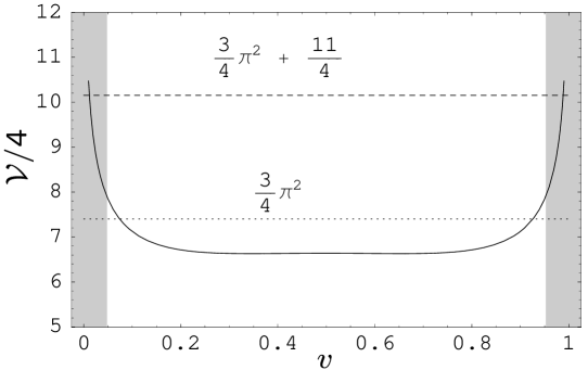
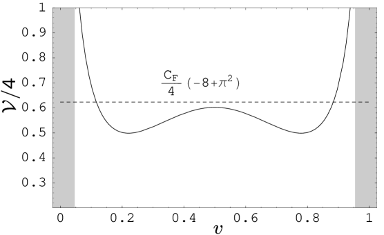
(a)                                                    (b)

Figure 1: Comparison of the functions ${\mathcal{V}}/4$ (a) for $gg\rightarrow\gamma\gamma$ (solid line) and Higgs boson production $gg\rightarrow H$ (dashed line); (b) for $q\bar{q}\rightarrow\gamma\gamma$ (solid line) and the Drell-Yan process $q\bar{q}\rightarrow V$ (dashed line). The shaded areas are excluded by the experimental cuts for $Q=120$ GeV.

It is interesting to note that the comparable corrections to the process $q\bar{q}\rightarrow\gamma\gamma$ are considerably smaller than for $gg\rightarrow\gamma\gamma$. In Fig. 1(b) we plot the analogous function ${\mathcal{V}}_{q\bar{q}\rightarrow\gamma\gamma}/4$ (i.e., the coefficient of the $\delta(1-x)$ term in ${{\mathcal{C}}}^{(1)}_{q/q}(x)$), which was given in Refs. [8, 11]. We see that it is equal to $0.5-0.6$ in most of the kinematical region selected by the LHC cuts, which is much less than the value of 6.65 that we found for the $gg$-initiated process. In this figure we also plot the analogous coefficient ${\mathcal{V}}_{DY}/4$ for the Drell-Yan process, which differs from ${\mathcal{V}}_{q\bar{q}\rightarrow\gamma\gamma}/4$ by less than $5-20\%$ over this kinematic range.

Since the function ${\mathcal{V}}_{gg\rightarrow\gamma\gamma}$ corrects only the $\delta(1-x)$ piece of ${{\mathcal{C}}}^{(1)}_{g/g}(x)$, and it does not depend on the impact parameter $b$, its primary effect is to change the overall normalization of the transverse momentum distribution, but not its shape. In Ref. [2], a K-factor was defined as the ratio of the NLO resummed cross section to the LO non-resummed cross section, using the corresponding PDFs in the numerator and denominator. By approximating the function ${\mathcal{V}}_{gg\rightarrow\gamma\gamma}$ by the analogous one for Higgs production, Eq. (10), the K-factor for the process $gg\rightarrow\gamma\gamma$ was estimated to be 1.45-1.75. We can now consider the impact of the correct function on the K-factor. Given that the contribution of $({{\mathcal{C}}}_{g/\Sigma}\otimes f_{\Sigma})(x,b;\mu_{F})$ constitutes less than $25\%$ of the contribution of $({{\mathcal{C}}}_{g/g}\otimes f_{g})(x,b;\mu_{F})$ in the central rapidity region, we estimate the correct $gg\rightarrow\gamma\gamma X$ K-factor to be about 1.2-1.5. Furthermore, we can use Fig. 2 in Ref. [2] to find the corrected K-factor for all included subprocesses to be about 1.3 at $Q=80$ GeV and 1.6 at $Q=150$ GeV. We note that the resummed K-factors for the $gg\rightarrow\gamma\gamma$ subprocess are slightly different than the fixed-order K-factors obtainable from Fig. 4(a) in Ref. [5]; however, this difference is primarily due to the fact that the renormalization scale was chosen to be $\mu_{0}=Q/2$ in Ref. [5] and that the different selection cuts used in that paper produced a kinematic enhancement of the K-factor for $Q$ near 80 GeV. Of course, these first estimates of the corrected resummed K-factors can be further refined by repeating a detailed Monte-Carlo study as in Ref. [2].

Recently, it has been shown that the remaining ${\mathcal{O}}(\alpha_{S}^{2}/\pi^{2})$ coefficient in the Sudakov factor, ${\mathcal{B}}^{(2)}$, can also be obtained from the NLO cross section, using the universality of the real emission corrections and the general structure of the virtual corrections in the soft and collinear limits [12]. Following this argument, we obtain

$${\mathcal{B}}_{gg\rightarrow X}^{(2)} = -\frac{\delta P_{g/g}^{(2)}}{2}+\beta_{0}\left(\frac{{\mathcal{V}}_{gg\rightarrow X}}{4}+\frac{N_{c}\pi^{2}}{12}\right)+\beta_{0}^{2}\ln\frac{\mu_{0}}{Q}$$ (11)

$$-2N_{c}\left(\left(\frac{67}{36}-\frac{\pi^{2}}{12}\right)N_{c}-\frac{5}{18}N_{f}\right)\ln\frac{b_{0}C_{2}}{C_{1}}$$

$$+\beta_{0}N_{c}\left(\left(\ln\frac{b_{0}}{C_{1}}\right)^{2}-\left(\ln C_{2}\right)^{2}\right)-\beta_{0}^{2}\ln C_{2},$$

which is valid both for Higgs boson production and diphoton production. In this formula the $\delta(1-x)$ part of the ${\cal O}(\alpha_{S}^{2})$ splitting function for $g\rightarrow g$ is

$$\delta P^{(2)}_{g/g}\,\,=\,\,N_{c}^{2}\left(\frac{8}{3}+3\zeta(3)\right)-\frac{1}{2}N_{f}C_{F}-\frac{2}{3}N_{f}N_{c}\,\,,$$ (12)

where $\zeta(n)$ is the Riemann zeta function, with $\zeta(3)=1.202057\dots$. For Higgs boson production, Eq. (11) has been corroborated by direct calculation from the NLO transverse momentum distributions [13]. In Fig. 2 we plot the ${\cal B}^{(2)}$ coefficient functions for various processes, with the canonical choice of parameters and $N_{f}=5$. From this plot, we see that ${\mathcal{B}}^{(2)}_{gg\rightarrow H}$ is almost exactly twice as large as ${\mathcal{B}}^{(2)}_{gg\rightarrow\gamma\gamma}$ over most of the allowed kinematic region, and both coefficients are considerably larger than those for the $q\bar{q}$-initiated processes.

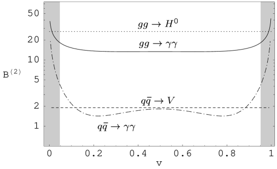
Figure 2: Comparison of the coefficient ${\mathcal{B}}^{(2)}$ in various particle reactions. The shaded areas are excluded by the experimental cuts for $Q=120$ GeV.

In the standard CSS formalism, the functions ${\mathcal{B}}$ and ${{\mathcal{C}}}_{g/a}$ are process-dependent, as seen explicitly above. Ref. [14] proposed a modified resummation formula, which removes from these functions all terms associated with hard virtual QCD corrections to the LO process. Such hard corrections are absorbed in a new function ${\mathcal{H}}(\alpha_{S})$, so that the alternate formula for $\widetilde{W}(b,Q,v,x_{A},x_{B})$ is

$$\widetilde{W}(b,Q,v,x_{A},x_{B})=\frac{\sigma_{0}(\alpha_{S}(\mu_{0}))}{S}{\mathcal{H}}(\alpha_{S}(\mu_{0}))$$

$$\times\exp\left\{-\int_{C_{1}^{2}/b^{2}}^{C^{2}_{2}Q^{2}}\frac{d\bar{\mu}^{2}}{\bar{\mu}^{2}}\Bigl{[}{\mathcal{A}}(\alpha_{S}(\bar{\mu}))\ln\frac{C_{2}^{2}Q^{2}}{\bar{\mu}^{2}}+{\mathcal{B}}^{\prime}(\alpha_{S}(\bar{\mu}))\Bigr{]}\right\}$$

$$\times\sum_{a,b}\left[{\mathcal{C}}^{\prime}_{g/a}\otimes f_{a}\right](x_{A},b;\mu_{F},\alpha_{S}(\mu_{F}))\left[{\mathcal{C}}^{\prime}_{g/b}\otimes f_{b}\right](x_{B},b;\mu_{F},\alpha_{S}(\mu_{F})).$$ (13)

Here we can expand ${\mathcal{B}}^{\prime}(\alpha_{S})$ and ${{\mathcal{C}}}^{\prime}_{g/a}(x,b;\mu_{F},\alpha_{S})$ as a series in $\alpha_{S}$ exactly as the functions ${\mathcal{B}}(\alpha_{S})$ and ${{\mathcal{C}}}_{g/a}(x,b;\mu_{F},\alpha_{S})$, and the function ${\mathcal{H}}(\alpha_{S})$ can similarly be expanded as ${\mathcal{H}}(\alpha_{S})\,\,=\,\,1+\sum_{n=1}^{\infty}\left({\alpha_{S}}/{\pi}\right)^{n}{\mathcal{H}}^{(n)}$.

In this formulation, there is a “scheme-dependent” ambiguity in the definition of ${{\mathcal{C}}}^{\prime}_{g/g}$, ${\mathcal{B}}^{\prime}$, and ${\mathcal{H}}$, since a change in ${\mathcal{H}}$ can be compensated by redefinitions of ${{\mathcal{C}}}^{\prime}_{g/g}$ and ${\mathcal{B}}^{\prime}$. A reasonable choice of scheme is to define

$${\mathcal{H}}^{(1)}_{gg\rightarrow X}\,\,=\,\,\frac{{\mathcal{V}}_{gg\rightarrow X}}{2}+2\beta_{0}\ln\frac{\mu_{0}}{Q},$$ (14)

so that ${\mathcal{C}}^{(1)\prime}_{g/g}(x)$ vanishes for the canonical choice of parameters. In this scheme, which is similar to the ‘NS resummation scheme’ of Ref. [14], we obtain

$${\mathcal{C}}^{(1)\prime}_{g/g}(x) = \delta(1-x)\left(-\beta_{0}\ln\frac{b_{0}C_{2}}{C_{1}}-N_{c}\ln^{2}\frac{b_{0}C_{2}}{C_{1}}\right)-P^{(1)}_{g/g}(x)\ln\frac{\mu_{F}b}{b_{0}}\,\,,$$ (15)

$${\mathcal{B}}_{gg\rightarrow X}^{(2)\prime} = -\frac{\delta P_{g/g}^{(2)}}{2}+\beta_{0}N_{c}\frac{\pi^{2}}{12}+\beta_{0}N_{c}\left(\left(\ln\frac{b_{0}}{C_{1}}\right)^{2}-\left(\ln C_{2}\right)^{2}\right)$$ (16)

$$-2N_{c}\left(\left(\frac{67}{36}-\frac{\pi^{2}}{12}\right)N_{c}-\frac{5}{18}N_{f}\right)\ln\frac{b_{0}C_{2}}{C_{1}}-\beta_{0}^{2}\ln C_{2}\,\,,$$

as well as ${\mathcal{B}}^{(1)^{\prime}}={\mathcal{B}}^{(1)}$ and ${{\mathcal{C}}}^{(1)\prime}_{g/\Sigma}(x)={{\mathcal{C}}}^{(1)}_{g/\Sigma}(x)$. The advantage of this formulation for diphoton production is that it allows us to shift all dependence on the kinematical variable $v$ from ${{\mathcal{C}}}^{\prime}_{g/g}$ and ${\mathcal{B}}^{\prime}$ into the single hard factor ${\mathcal{H}}$. This choice makes sense physically, since this kinematical dependence is a property of the hard $gg\rightarrow\gamma\gamma$ process, rather than of soft or collinear effects. This formulation also makes more obvious the fact that the function ${\mathcal{V}}_{gg\rightarrow\gamma\gamma}$ affects the normalization, but not the shape, of the transverse momentum distribution. A similar modification can be made to the $q\bar{q}\rightarrow\gamma\gamma X$ resummation formula.

In conclusion, we have calculated the remaining unknown parts at ${\mathcal{O}}(\alpha_{S}/\pi)$ in the resummed cross section for the production of photon pairs in gluon-gluon fusion at small $Q_{T}$. We found that the approximation of the function ${{\mathcal{C}}}_{g/g}(x,b;\mu_{F})$ in the process $gg\rightarrow\gamma\gamma$ by its counterpart from Higgs boson production overestimates the $gg\rightarrow\gamma\gamma X$ resummed K-factor by about $15-20\%$, and it overestimates the K-factor for the total diphoton production process by about $5-10\%$. We have also calculated the ${\mathcal{O}}(\alpha_{S}^{2}/\pi^{2})$ coefficient ${\mathcal{B}}^{(2)}$ in the perturbative Sudakov factor. We predict that the impact of the coefficient ${\mathcal{B}}^{(2)}$ on the shape of transverse momentum distributions in gluon fusion is more substantial then in the process $q\bar{q}\rightarrow\gamma\gamma$, and that it will improve the matching of the resummed calculation with the fixed-order calculation at intermediate $Q_{T}$ .