SLAC-PUB-9596 November 2002

Phenomenology on a Slice of $AdS_{5}\times{\cal M}^{\delta}$ Spacetime

H. Davoudiasl¹, J.L. Hewett², and T.G. Rizzo²

¹School of Natural Sciences, Institute for Advanced Study, Princeton, NJ 08540

²Stanford Linear Accelerator Center, Stanford, CA, 94309

We study the phenomenology resulting from backgrounds of the form $AdS_{5}\times{\cal M}^{\delta}$, where ${\cal M}^{\delta}$ denotes a generic manifold of dimension $\delta\geq 1$, and $AdS_{5}$ is the slice of 5-dimensional anti-de Sitter space which generates the hierarchy in the Randall-Sundrum (RS) model. The $\delta$ additional dimensions may be required when the RS model is embedded into a more fundamental theory. We analyze two classes of $\delta-$dimensional manifolds: flat and curved geometries. In the first case, the additional flat dimensions may accommodate localized fermions which in turn could resolve issues, such as proton decay and flavor, that were not addressed in the original RS proposal. In the latter case, the positive curvature of an $S^{\delta}$ manifold with $\delta>1$ can geometrically provide the 5-dimensional warping of the RS model. We demonstrate the key features of these two classes of models by presenting the background solutions, the spectra of the Kaluza-Klein (KK) gravitons, and their 4-dimensional couplings, for the sample manifolds $S^{1}/Z_{2}$, $S^{1}$, and $S^{2}$. The resulting phenomenology is distinct from that of the original RS scenario due to the appearance of a multitude of new KK graviton states at the weak scale with couplings that are predicted to be measurably non-universal within the KK tower. In addition, in the case of flat compactifications, fermion localization can result in KK graviton and gauge field flavor changing interactions.

1 Introduction

In the Randall-Sundrum (RS) model [1], the hierarchy between the electroweak and gravitational scales is explained in the context of a 5-dimensional (5-d) background geometry, which is a slice of anti-de Sitter ($AdS_{5}$) spacetime. Two 3-branes of equal and opposite tension sit at orbifold fixed points at the boundaries of the $AdS_{5}$ slice. We denote this geometrical setup as $|AdS_{5}|$ to emphasize that it consists of a slice of anti-de Sitter space. The 5-d warped geometry induces a 4-d effective scale $\Lambda_{\pi}$ of order a TeV on one of the branes. $\Lambda_{\pi}$ is thus exponentially smaller than the gravitational scale, which is given by the reduced Planck mass $\overline{M}_{Pl}$. In this scenario, parameters of the 5-d theory maintain their natural size, of order $\overline{M}_{Pl}$, even though the 4-d picture has hierarchical mass scales with $\Lambda_{\pi}/\overline{M}_{Pl}\sim 10^{-15}$. The RS proposal has distinct phenomenological signatures that are expected to be revealed in experiments at the TeV scale, and hence the phenomenology of this model has been studied in detail [2, 3].

From a more theoretical perspective, one may view the RS model as an effective theory whose low energy features originate from a full theory of quantum gravity, such as string theory. Based on this view, and also on general grounds, one may expect that a more complete version of this scenario must admit the presence of additional extra dimensions compactified on a manifold ${\cal M}^{\delta}$ of dimension $\delta$. From a model building point of view, it can be advantageous to place at least some of the Standard Model (SM) fields in the higher dimensional space. This possibility generally allows for new model-building techniques to address gauge coupling unification [4], supersymmetry breaking [5], and the neutrino mass spectrum [6]. However, the placement of SM fields in the RS $|AdS_{5}|$ bulk is problematic due to large contributions to precision electroweak observables arising from the SM Kaluza-Klein (KK) states [3]. Hence the presence of the additional manifold may reconcile these model building features with the RS model. For example, in the RS model, despite its interesting features, the issues of proton decay and flavor do not have a simple explanation. However, these problems are naturally addressed in simple geometries, such as an $S^{1}/Z_{2}$ extra dimension along which fermion fields are localized [7]. Thus, considering an $|AdS_{5}|\times S^{1}/Z_{2}$ background, for example, can in a straightforward way provide the RS model with a geometrical explanation of proton stability and flavor, while preserving the desirable features of its description of the hierarchy.

Given the motivation for considering an extended $|AdS_{5}|\times{\cal M}^{\delta}$ background, it is then interesting to determine how the original RS phenomenology is modified in the presence of the additional manifold and what new signatures can be expected in future experiments. Other studies of extended RS scenarios [8] have focused on the mechanism for localizing gravity on a thick brane or on a singular string-like defect, but have not examined the resulting phenomenology. In this work, we examine the phenomenology resulting from two classes of additional geometries; flat and curved spaces. We consider the manifolds $S^{\delta}$, with $\delta\geq 1$, as this choice has the advantage of simplicity and provides a representative example of each class of geometry. The flat case with $\delta=1$ provides a natural mechanism for addressing proton decay and flavor as discussed above. For $\delta>1$, the extra manifold $S^{\delta}$ has positive curvature and we elucidate how this curvature can serve as the origin of the warping in the 5-d RS picture. We expect that the qualitative features of our results obtained from $S^{\delta}$ are representative of the phenomenology for fairly general choices of the manifold ${\cal M}^{\delta}$.

We find that the addition of the $S^{\delta}$ background to the RS setup typically results in the emergence of a forest of graviton KK resonances ocurring in between the original RS resonances. This forest originates from the ‘angular’ excitations on the $S^{\delta}$. In this paper, we focus mainly on the derivation of the graviton KK spectrum, and study the cases ${\cal M}=S^{1},S^{1}/Z_{2}$, and $S^{2}$ in some detail. We address the constraints placed by data on this picture, as well as issues related to the extraction of model parameters from experimental data. In the scenario where the SM fermions are localized in the $S^{1}/Z_{2}$ manifold, we note that flavor changing graviton interactions may arise at the tree-level, which could in principle pose a threat to this model. We give an estimate for such contributions and find that they do not occur at a dangerous level. We note that in $d>5$, gravi-scalars and gravi-vectors [9] also play a role in weak scale phenomenology, especially if the SM fields reside in the $S^{\delta}$, but we do not consider the modifications from these sectors here.

In the next two sections, we present the background solutions for the flat and curved geometries, corresponding to $\delta=1,2$, respectively. In each case, we examine the resulting spectrum of the KK gravitons and compute their couplings to 4-d fields. We then present our results for the expected production cross sections of the KK gravitons at colliders, as well as the associated experimental bounds. Lastly, we comment on the case where the SM fields can propagate in the $S^{\delta}$, and outline some of the issues that need further study in this case. We present our conclusions in section 4.

2 The Graviton KK Spectrum and Couplings: Flat Manifolds

For simplicity, we limit our study to the flat manifolds $S^{1}$ and $S^{1}/Z_{2}$; our results easily generalize to the case of other toroidal compactifications. We first discuss the boundary conditions that lead to the $|AdS_{5}|\times S^{1}$ background and derive the 4-d spectrum of the corresponding KK gravitons and their couplings. We then study the phenomenology of the KK graviton spectrum and discuss some consequences of placing the SM fermions in the additional manifold.

2.1 Formalism

The metric for the $|AdS_{5}|\times S^{1}$ background is given by

$$ds^{2}=e^{-2\sigma}\eta_{\mu\nu}dx^{\mu}dx^{\nu}+r_{c}^{2}\,d\phi^{2}+R^{2}\,d\theta^{2},$$ (1)

where, following the conventions and notation of Ref.[1], we have $\sigma=kr_{c}|\phi|$, with $k>0$ setting the scale of the curvature of the $AdS_{5}$ slice. The ‘radial’ (RS) dimension, $x_{4}$, is parameterized as $x_{4}=r_{c}\phi$ by the angle $\phi\in[-\pi,\pi]$, where $r_{c}$ is the compactification radius. The two 4-branes sit at the orbifold fixed points $\phi=0,\pi$. The $S^{1}$ is parameterized by the angle $\theta\in[0,2\pi]$, and $R$ is the radius of the $S^{1}$. To obtain a solution to Einstein’s equation corresponding to this metric, we need the inhomogeneous cosmological constant tensor and the energy-momentum tensor for the sources on the branes [10]. For the cosmological constant tensor, we choose

$$\Lambda^{A}_{B}={\rm diag}(\Lambda,\Lambda,\Lambda,\Lambda,\Lambda,\Lambda_{\theta}),$$ (2)

and the energy-momentum tensor is assumed to have the form

$$T^{M}_{N}=-\left\{\delta(\phi)\left(\begin{array}[]{ccc}V^{h}\delta^{\mu}_{\nu}&0&0\cr 0&0&0\cr 0&0&V_{\theta}^{h}\end{array}\right)+\delta(\phi-\pi)\left(\begin{array}[]{ccc}V^{v}\delta^{\mu}_{\nu}&0&0\cr 0&0&0\cr 0&0&V_{\theta}^{v}\end{array}\right)\right\},$$ (3)

with $V$ representing the brane tensions where the superscripts $v$ and $h$ correspond to the visible and hidden branes, respectively.

In a fashion similar to that in Ref.[1], we can then solve Einstein’s equations for the above setup, and obtain the following results

$$V^{h}=-V^{v}=-\Lambda/k=24\,M_{F}^{4}\,k,$$ (4)

and

$$\Lambda=\frac{3}{5}\,\Lambda_{\theta}\,\,;\,\,V^{h}=\frac{3}{4}\,V^{h}_{\theta}\,\,;\,\,V^{v}=\frac{3}{4}\,V^{v}_{\theta}\,,$$ (5)

where $M_{F}$ denotes the 6-dimensional fundamental scale. Following the conventions of Ref.[1], we have

$$\overline{M}_{Pl}^{2}=\int_{-\pi}^{+\pi}r_{c}\,d\phi\int_{0}^{2\pi}R\,d\theta\,e^{-2\sigma}M_{F}^{4},$$ (6)

from which we derive the following relation

$$\overline{M}_{Pl}^{2}=\frac{2\pi R}{k}\,M_{F}^{4}[1-e^{-2\sigma(\pi)}].$$ (7)

We now discuss the derivation of the KK spectrum. In the rest of this work, we will limit our analysis to the case of metric perturbations of the form

$$G_{\mu\nu}=e^{-2\sigma}(\eta_{\mu\nu}+\kappa\,h_{\mu\nu}),$$ (8)

where $\kappa=2/M_{F}^{(3+\delta)/2}$, and $M_{F}$ is the fundamental scale in $(5+\delta)$ dimensions. Our background solutions for $S^{1}$ and $S^{2}$ follow from the original RS convention, except for our choice of $\kappa$, since it is assumed that the coefficient of the 5-d curvature term is $\kappa^{-2}$. The gauge choice for all our computations is the transverse traceless gauge; $\partial^{\mu}h_{\mu\nu}=h^{\mu}_{\mu}=0$. We choose the following KK expansion for $h_{\mu\nu}$ in Eq.(8)

$$h_{\mu\nu}(x,\phi,\theta)=\sum_{n,l}h^{(n,\,l)}_{\mu\nu}(x)\frac{\chi^{(n,\,l)}(\phi)}{\sqrt{r_{c}}}\frac{\varphi^{(l)}(\theta)}{\sqrt{R}}.$$ (9)

The $\theta-$dependent wavefunction is given by

$$\varphi^{(l)}(\theta)=e^{il\theta}/{\sqrt{2\pi}}$$ (10)

in the case of $S^{1}$ and

$$\varphi^{(l)}(\theta)=\left\{\begin{array}[]{ll}{1/\sqrt{2\pi}},&\quad l=0\\ {\cos l\theta/\sqrt{\pi}},&\quad l\neq 0\end{array}\right.$$ (11)

for the orbifolded case $S^{1}/Z_{2}$. Inserting the above KK expansion in the perturbed Einstein’s equations, we find, to linear order in $\kappa$, the following eigenvalue equation for the $(n,\,l)$ mode with mass $m_{nl}$

$$-\frac{1}{r_{c}^{2}}\frac{d}{d\phi}\left(e^{-4\sigma}\frac{d}{d\phi}\chi^{(n,\,l)}(\phi)\right)+e^{-4\sigma}\left(\frac{l}{R}\right)^{2}\chi^{(n,\,l)}(\phi)=e^{-2\sigma}m_{nl}^{2}\chi^{(n,\,l)}(\phi).$$ (12)

This is the equation of motion in the RS model for a bulk scalar field of 5-d mass $l/R$. The solutions are given by [11]

$$\chi^{(n,\,l)}_{l}(\phi)=\frac{e^{2\sigma}}{N_{nl}}\,[J_{\nu}(z_{nl})+\alpha_{nl}Y_{\nu}(z_{nl})],$$ (13)

where $J_{\nu}$ and $Y_{\nu}$ denote Bessel functions of order $\nu$. We now find

$$\nu\equiv\sqrt{4+\left(\frac{l}{kR}\right)^{2}}$$ (14)

with $z_{nl}(\phi)\equiv(m_{nl}/k)e^{\sigma}$. (We will ignore terms suppressed by powers of $e^{-kr_{c}\pi}$ throughout our computations.) The normalization $N_{nl}$ is then given by

$$N_{nl}=\frac{e^{kr_{c}\pi}}{\sqrt{kr_{c}}}J_{\nu}(x_{nl})\sqrt{1+\left(\frac{4-\nu^{2}}{x_{nl}^{2}}\right)},$$ (15)

where $x_{nl}=z_{nl}(\pi)$. The $x_{nl}$ are solutions of the equation

$$2J_{\nu}(x_{nl})+x_{nl}J_{\nu}^{\prime}(x_{nl})=0,$$ (16)

which yields the masses $m_{nl}$. There are no modes for which $l\neq 0$ and $\chi^{(n,\,l)}(\phi)=$ Constant, i.e., for $n=0$, only the case $l=0$ is allowed. This means that all KK graviton states have warp-factor enhanced couplings, as in the original RS model. The zero mode, corresponding to the massless 4-d graviton, has the wavefunction $\chi^{(0,\,0)}=\sqrt{kr_{c}}$.

Since we are interested in the situation where the SM fields are localized on the circle, we consider, for simplicity, the case where they are placed at $\theta=0$. For either $S^{1}$ or $S^{1}/Z_{2}$, the results for the graviton couplings derived below can be easily generalized to the case $\theta=\theta_{0}$, with $\theta_{0}$ being arbitrary, as will be discussed in section 2.4.2. The 6-d graviton coupling to the energy momentum tensor of 4-d fields localized at $\phi=\pi$ and $\theta=0$ is given by

$${\cal L}=-\frac{1}{M_{F}^{2}}h^{\mu\nu}(x,\pi,0)T_{\mu\nu}(x).$$ (17)

Substituting the KK expansion (9) in the above, and using the expressions for $\chi^{(n)}_{l}(\phi)$ and $N_{n}$, yields

$${\cal L}=-\frac{1}{\overline{M}_{Pl}}h_{\mu\nu}^{(0,\,0)}(x)T^{\mu\nu}(x)-\frac{1}{\Lambda_{\pi}}T^{\mu\nu}(x)\sum_{l=-\infty}^{\infty}\sum_{n=1}^{\infty}\xi(n,l)h_{\mu\nu}^{(n,\,l)}(x)$$ (18)

for the case of $S^{1}$, and

$${\cal L}=-\frac{1}{\overline{M}_{Pl}}h_{\mu\nu}^{(0,\,0)}(x)T^{\mu\nu}(x)-\frac{1}{\Lambda_{\pi}}T^{\mu\nu}(x)\sum_{l=0}^{\infty}\sum_{n=1}^{\infty}C_{l}\,\xi(n,l)h_{\mu\nu}^{(n,\,l)}(x)$$ (19)

for the orbifolded case $S^{1}/Z_{2}$. Here, $\Lambda_{\pi}\equiv e^{-kr_{c}\pi}\overline{M}_{Pl}$,

$$\xi(n,l) = \left[1-\left(\frac{l}{kRx_{nl}}\right)^{2}\right]^{-1/2}\,,$$

$$C_{l} = \left\{\begin{array}[]{cl}1,&\quad l=0\\ \sqrt{2},&\quad l\neq 0\end{array}\right.\,.$$ (22)

The massless zero mode graviton couples with the 4-d strength $1/\overline{M}_{Pl}$, as required. We note that the coupling of various KK gravitons to the 4-d energy-momentum tensor is not universal. This non-universality, with natural choices of parameters, could be of ${\cal O}(1)$ for the light KK modes, and would be easily measured in experiment. This is in contrast to the case of the original RS scenario where the non-universality is suppressed by ${\cal O}(e^{-kr_{c}\pi})$ for the light modes [2]. Note that since $x_{nl}>l/kR$, the factor $\xi{(n,l)}$ is always real.

2.2 Discussion of Model Parameters

Here, we discuss the parameters present in this scenario and their relation to the phenomenological features of the graviton KK spectrum. In the original RS model[1], the two parameters can be chosen to be the mass of the first graviton resonance (or, alternatively, $\Lambda_{\pi}$) and the ratio $k/\overline{M}_{Pl}$. The desire that there be no new hierarchies suggests that $k/\overline{M}_{Pl}\mathrel{\mathchoice{\lower 3.01385pt\vbox{\halign{$\matth\displaystyle\hfil#\hfil$\cr>\crcr\sim\crcr}}}{\lower 3.01385pt\vbox{\halign{$\matth\textstyle\hfil#\hfil$\cr>\crcr\sim\crcr}}}{\lower 3.01385pt\vbox{\halign{$\matth\scriptstyle\hfil#\hfil$\cr>\crcr\sim\crcr}}}{\lower 3.01385pt\vbox{\halign{$\matth\scriptscriptstyle\hfil#\hfil$\cr>\crcr\sim\crcr}}}}10^{-2}$ while the validity of the classical approximation leads to the requirement that the 5-dimensional curvature satisfy $|R_{5}|\leq\overline{M}_{Pl}^{2}$ which, in turn, implies $k/\overline{M}_{Pl}\,\,\hbox to0.0pt{\raise 3.0pt\hbox{$<$}\hss}{\lower 3.0pt\hbox{$\sim$}}\,\,0.1$ [2, 3]. In the present scenario, there is an additional parameter, $R$, describing the radius of the circle $S^{1}$ or the orbifold $S^{1}/Z_{2}$. The corresponding consideration of the 6-dimensional curvature, $R_{6}$, yields the same bound as above on the ratio $k/\overline{M}_{Pl}$ while giving no constraint on $R$. However, naturalness and the wish that no new hierarchies exist suggests that the value of the mass scale $R^{-1}$ not be very different from $k$, $\overline{M}_{Pl}$ or the fundamental scale $M_{F}$. To be specific, we will assume that $0.1\,\,\hbox to0.0pt{\raise 3.0pt\hbox{$<$}\hss}{\lower 3.0pt\hbox{$\sim$}}\,\,kR\,\,\hbox to0.0pt{\raise 3.0pt\hbox{$<$}\hss}{\lower 3.0pt\hbox{$\sim$}}\,\,10$ in our numerical analysis below; this range is sufficient to demonstrate the features of the new physics associated with the $S^{1}(/Z_{2})$ extension to the original RS model. As we will see below, the value of $R$ is intimately connected with the shape of the KK spectrum in the present scenario.

Before discussing our results, we first examine the qualitative features of the KK spectrum in the present scenario. For convenience, we label the states and their corresponding masses by the values of the integers $n$ and $l$, as denoted in the previous section. This notation suggests that $(n,\,l)$ play a role similar to the quantum numbers in atomic structure considerations. The states $l=0$ for any $n$ correspond to the KK states in the original RS construction. In addition, as we saw above, for $n=0$ only $l=0$ is allowed, but for any $n\geq 1$, states with $l\geq 0$ exist.

To gain an understanding of the KK spectrum a short numerical analysis shows that we may write the roots $x_{nl}$, which determine the KK tower masses, in the empirical form

$$x_{nl}^{2}\simeq\Bigg{[}x_{n}^{2}+{x_{n}l\over{kR}}+\bigg{(}{l\over{kR}}\bigg{)}^{2}\Bigg{]}\,,$$ (23)

where the $x_{n}$ are the roots of $J_{1}$, i.e., $J_{1}(x_{n})=0$, and describe the KK spectrum in the original RS scenario [2]. This expression is justified by the behavior of the roots as a function of $l$ as shown in Fig. 1. Clearly, in this figure, only integral values of $l$ correspond to the physical situation. Note that the term linear in $x_{n},\,l$ in the above expression does not appear in the conventional case of two dimensional toroidal compactifications and has the appearance of a ‘cross-term’ between the contributions from the two geometrically different dimensions. This behavior also appears in the similar situation where the extra dimensional shape and moduli are both considered [12].

A more complete analysis of the roots $x_{nl}$ in this scenario confirms the qualitative features of the above empirical form for the KK tower masses. We have derived the behavior of the roots using asymptotic forms for the Bessel functions. In the limit of large $kR$, we find

$$x^{2}_{nl}\simeq x_{n}^{2}+{x_{n}\pi\over 4}\bigg{(}{l\over kR}\bigg{)}^{2}\,,$$ (24)

whereas, for small values of $kR$,

$$x^{2}_{nl}\simeq\Bigg{[}x_{n}+{\pi l\over 2kR}\Bigg{]}^{2}\,.$$ (25)

Note the appearance of the cross term in these limits. We find that these expressions provide a fairly accurate approximation to the full numerical results for the roots in these two limiting cases.

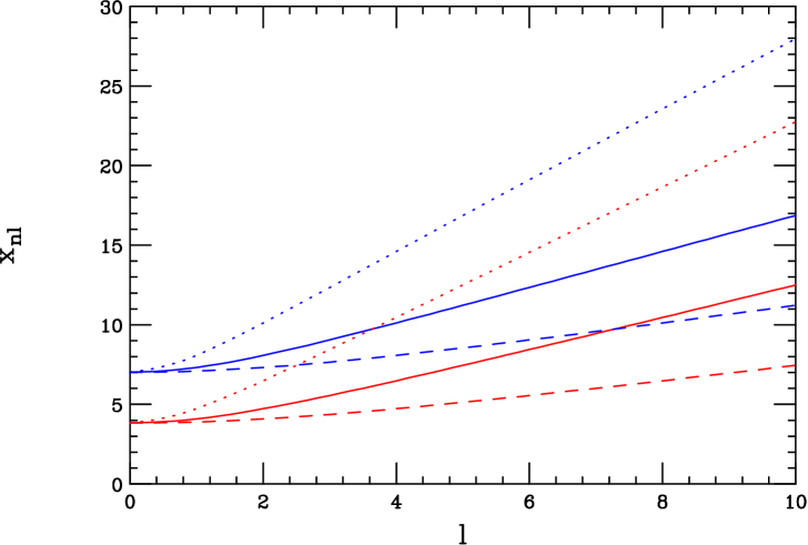
Figure 1: The roots $x_{nl}$ for $n=1,2$ as a function of $l$. The dotted, solid, dashed curves correspond to $kR=0.5,\,1.0,\,2.0$, respectively.

We now discuss the consequences of the above expression; in particular, there are two limiting cases which may hinder the observation of this scenario at colliders. When $(kR)^{-1}$ is large in comparison to $x_{n}$, the first $l$ excitation is heavy in comparison to the $l=0$ state, i.e., $m_{n1}/m_{n0}$ is large. This is due to the dominance of the quadratic term. If this mass ratio is too large, it is possible that the $l\geq 1$ KK states will be too massive to be produced directly at colliders. Colliders such as the LHC will thus only observe the KK graviton mass spectrum that is present in the usual RS model. Fortunately, a short analysis indicates that this is unlikely as long as $kR\mathrel{\mathchoice{\lower 3.01385pt\vbox{\halign{$\matth\displaystyle\hfil#\hfil$\cr>\crcr\sim\crcr}}}{\lower 3.01385pt\vbox{\halign{$\matth\textstyle\hfil#\hfil$\cr>\crcr\sim\crcr}}}{\lower 3.01385pt\vbox{\halign{$\matth\scriptstyle\hfil#\hfil$\cr>\crcr\sim\crcr}}}{\lower 3.01385pt\vbox{\halign{$\matth\scriptscriptstyle\hfil#\hfil$\cr>\crcr\sim\crcr}}}}0.05$ and hence lies within our natural range of values. On the otherhand, in the case where $kR$ is large, the $l$ excitations for a given $n$ will be very close in mass to the $l=0$ mode and will have a tendency to pile up near this state. Here, the separations between the $l$ excitations are tiny (yet growing with $l$), and may be too small to be observed at colliders. It is possible that the individual peaks would not be isolated in the data and information about the individual states would be lost. As we will see below, this is not a problem for the natural range of $kR$ that we have assumed, however, if $kR$ lies outside of this range, this issue will emerge.

2.3 Numerical Results

We first present the numerical results for the case where the additional dimension is orbifolded, $S^{1}/Z_{2}$. Fig. 2 displays the spectrum of KK graviton excitations that would be observed at an $e^{+}e^{-}$ collider via the process $e^{+}e^{-}\rightarrow\mu^{+}\mu^{-}$. Here, we assume $m_{10}=600$ GeV, $k/\overline{M}_{Pl}=0.03$ and $kR=1$; we will take this to be our reference set of parameter values in our discussions below. We note that the mass of the first graviton KK excitation is consistent with bounds from the Tevatron data sample [2]. The conventional KK graviton spectrum in the original RS scenario is shown for purposes of comparison. In performing these calculations we have made a simplifying assumption which only influences the KK states at or above the $n=3,\,l=0$ mode. These heavy states are allowed to decay to other KK modes [13] (note that the value of $l$ would need to be conserved in these decays due to orthonormality of the wavefunctions) and are thus wider than assumed in the present analysis which only includes decays to SM fields. Such potential decay channels include not only gravitons but also the gravi-vectors and gravi-scalars which remain after the KK decomposition. The latter modes are not present in the conventional RS model, as in that case the physical spectrum consists solely of the graviton KK tower and the radion. However, for six (or more) dimensions other physical states [9] remain after the KK decomposition; for $N$ extra dimensions there are $N-1$ physical gravi-vector KK towers as well as ${1\over{2}}N(N-1)$ physical gravi-scalar KK towers. When the resonant gravitons decay to these states they will generally appear as missing energy at a collider. With the SM fields confined to the orbifold fixed points as discussed above, these additional fields either do not couple to those of the SM or are coupled sufficiently weakly that their effects can be safely ignored in the present discussion. Our neglect of these additional channels is also validated by the fact that the lighter modes below the $n=3,\,l=0$ state are most likely to be the ones within kinematic reach at colliders. When $N\geq 1$, the exchange of these gravi-scalar and gravi-vector states may contribute to the KK graviton spectrum when the SM fields are not located at the orbifold fixed points.

A number of features can be observed from Fig. 2: ($i$) The density of the KK spectrum has substantially increased in comparison to the original RS model and now resembles a ‘forest’ of peaks, similar to the lines that appear in an atomic spectrum. Given the assumed value $kR=1$, both $n$ and $l$ excitations are present in the same kinematic region. There are 19 KK states appearing in the kinematical range displayed in this figure! ($ii$) The peaks are generally well separated except where accidental overlaps occur, e.g., the $n=1,\,l=5$ and $n=2,\,l=0$ states are essentially degenerate for this choice of parameters. Some overlap also occurs in the case of the more massive states due to their larger widths. ($iii$) Overall, the cross section at large $\sqrt{s}$ rises faster in the present scenario than in the usual RS model due to the large number of states; this may lead to early violations of unitarity and will be discussed further below. $(iv)$ The properties of the lowest lying KK state ($n=1,\,l=0$) are not altered significantly from that found in the conventional RS model; its width can then be used to extract the value of the parameter $k/\overline{M}_{Pl}$ in the usual manner [14].

We have checked whether the rise in the cross section for large values of $\sqrt{s}$ leads to early violation of unitarity. The partial wave unitarity bound [9] on the cross section for $2\rightarrow 2$ scattering of inital and final state fermions with helicity of 1 is given by

$$\sigma_{U}={20\pi\over s}=24.4\times 10^{6}\Bigg{[}{1{\rm TeV}\over\sqrt{s}}\Bigg{]}^{2}{\rm fb}\,.$$ (26)

We employ the criteria that the cross section be well behaved up to the ultra-violet scale in this theory, i.e., $\Lambda_{\pi}$. For this set of parameters we have $\Lambda_{\pi}\simeq 5$ TeV, and we see that unitarity is violated as $\sqrt{s}$ closely approaches this value. Either the ultra-violet effects must set in slightly below $\Lambda_{\pi}$, or this set of parameters results in a mild violation of unitarity. We will return to this point below when examining the variation of the KK spectrum with the model parameters.

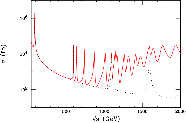
Figure 2: The solid red curve corresponds to the cross section for $e^{+}e^{-}\rightarrow\mu^{+}\mu^{-}$ when the additional dimension is orbifolded, i.e., for $S^{1}/Z_{2}$, with $m_{10}=600$ GeV, $k/\overline{M}_{Pl}=0.03$ and $kR=1$ being assumed. The result for the conventional RS model is also displayed, corresponding to the dotted curve.

Such a forest of KK graviton resonances may also be clearly seen at the LHC. Fig. 3 shows a histogram of the Drell-Yan cross section into $e^{+}e^{-}$ pairs, including detector smearing [15] and assuming the same model parameters as above except for $m_{10}=1$ TeV. The individual peaks at smaller masses are well separated except where they are nearly degenerate due to this choice of model parameters. At larger masses there is increased overlap among the KK states and individual resonances may be difficult to isolate. A detailed detector study of this KK forest is required to determine what separation between the states is necessary in order to isolate the resonances.

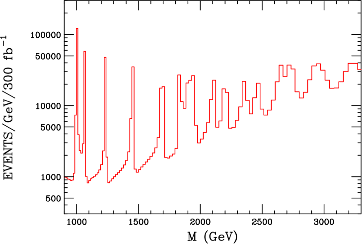
Figure 3: Binned Drell-Yan cross section for $e^{+}e^{-}$ production at the LHC assuming $m_{10}=1$ TeV and all other parameters as in Fig. 2. The cross section has been smeared by an electron pair mass resolution of $0.6\%$ as might be expected at ATLAS [15].

We now study the variations in these results for different choices of the model parameters. In the original RS scenario, the widths of the individual KK graviton resonances, as well as the interferences between the various peaks, are determined by the parameter $k/\overline{M}_{Pl}$. Increasing $k/\overline{M}_{Pl}$ leads to larger widths in the present scenario as well, but given the rather dense forest of KK excitations, the individual states will now tend to overlap thus smearing out the cross section. To demonstrate this effect, we consider the same case as above but now take $k/\overline{M}_{Pl}=0.1$; the resulting spectrum in $e^{+}e^{-}\rightarrow\mu^{+}\mu^{-}$ is displayed in Fig. 4. Here we see that the states above $n=2,l=0$ can no longer be resolved into individual peaks and yield a smoothly rising cross section. Note that the state $n=1,l=4$ is barely observable. Below this state, while the individual resonances are separated, their shapes are distorted due to the strong interference between the excitations. This is particularly clear in the case of the $n=1,l=0$ state which is likely to be too deformed to allow for a simple extraction of the value of $k/\overline{M}_{Pl}$. In this case, we now find that the unitarity bound in Eq. (26) is indeed preserved up to the scale $\Lambda_{\pi}$, which is given by $\sim 1.5$ TeV for this set of parameters.

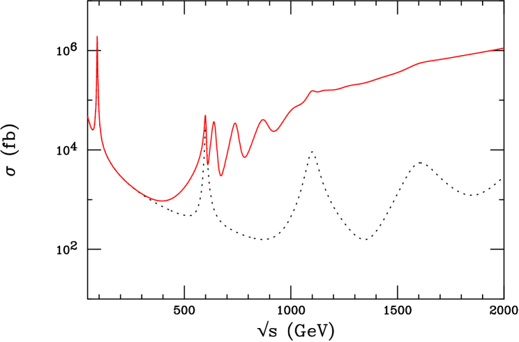
Figure 4: The solid red curve corresponds to the cross section for $e^{+}e^{-}\rightarrow\mu^{+}\mu^{-}$ when the additional dimension is orbifolded, i.e., for $S^{1}/Z_{2}$, with $m_{10}=600$ GeV, $k/\overline{M}_{Pl}=0.1$ and $kR=1$ being assumed. The result for the conventional RS model is also displayed, corresponding to the dotted curve.

Next we consider varying the values of $kR$; from Eq.(23) we see that $kR$ need not be too far away from unity in order to obtain significant modifications in the results shown above. Here we consider the cases $kR=0.5$ and 2 which yield the results shown in Fig. 5. For $kR=0.5$ the states are more widely separated than when $kR=1$ and the individual peaks would be easily observed and studied in a collider detector. If the value of $kR$ were further reduced, the $l\neq 0$ excitations would quickly grow heavier, e.g., setting $kR=0.05(0.1)$ gives the ratio $m_{11}/m_{10}=5.94(3.26)$ which, for the first case, is significantly beyond the kinematic range shown in the figure. If the energy range of the collider were restricted in comparison to such a spectrum, the $l$ excitations would go unobserved. As the value of $kR$ increases, the resonance forest grows thicker and dozens of states are seen to at least partially overlap when $kR$ reaches a value of 2. Note that the spacing between the $n=1,l=0$ and the $n=l=1$ state is rather small in this case, being only 425 MeV; this is comparable to their individual widths which are $\simeq 525$ MeV. The $\mu$-pair mass resolution at a linear collider should be sufficient to resolve these two states if they are within kinematic reach. However, if the value of $kR$ is increased further, separation of these first two states may prove difficult, especially for values of $kR$ as large as 10 or more where the peaks would be separated by less than 100 MeV.

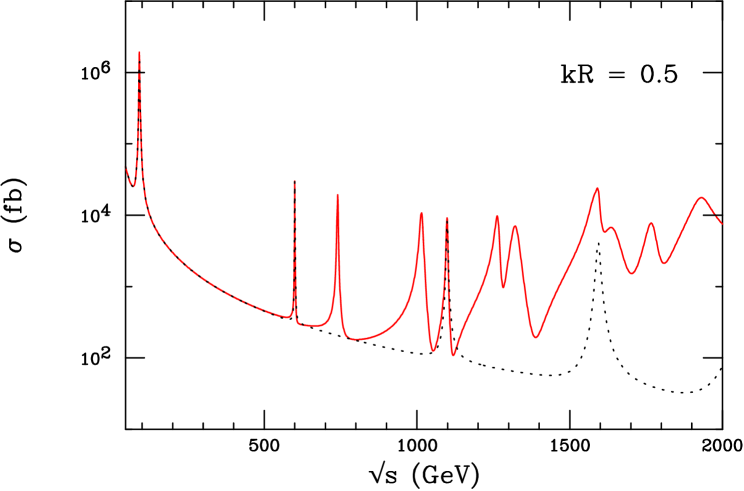
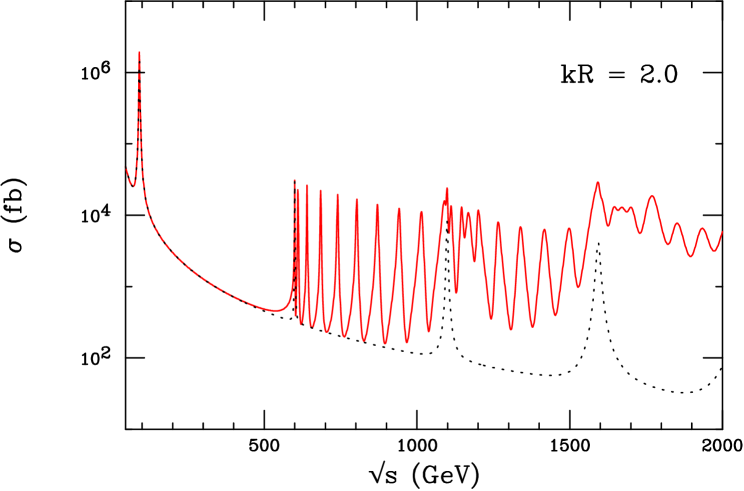
Figure 5: The solid red curve corresponds to the cross section for $e^{+}e^{-}\rightarrow\mu^{+}\mu^{-}$ when the additional dimension is orbifolded, i.e., for $S^{1}/Z_{2}$, with $m_{10}=600$ GeV, $k/\overline{M}_{Pl}=0.03$ and $kR=0.5$ (top), $kR=2.0$ (bottom) being assumed. The result for the conventional RS model is also displayed, corresponding to the dotted curve.

Lastly, we consider the scenario where we do not orbifold the $S^{1}$. In this scenario, the eigenfunctions and the resulting couplings are modified as discussed above. Recall that in the case of $S^{1}/Z_{2}$, the eigenfunctions take the form $\sim\cos l\theta$ (with $l\geq 0$) and are normalized such that an additional factor of $\sqrt{2}$ occurs in couplings when $l>0$. This is similar to the familiar results of TeV-scale extra-dimensional theories with bulk SM fields. Without orbifolding, the eigenfunctions are of the form $\sim e^{il\theta}$, with $l$ of either sign, and the extra factor of $\sqrt{2}$ does not appear in the normalization. Thus we can treat each level with $|l|>0$ as doubly degenerate, in contrast to the $S^{1}/Z_{2}$ case where no degeneracy occurs. The results for the non-orbifolded case, taking these factors into account, are shown in Fig. 6. Except for interference effects, we see that the $l=0$ resonances are identical in the two cases whereas $l\neq 0$ excitations are much more pronounced due to the double degeneracy. Since there are essentially twice as many states, the overall cross section increases much more rapidly with $\sqrt{s}$ than in the orbifolded case.

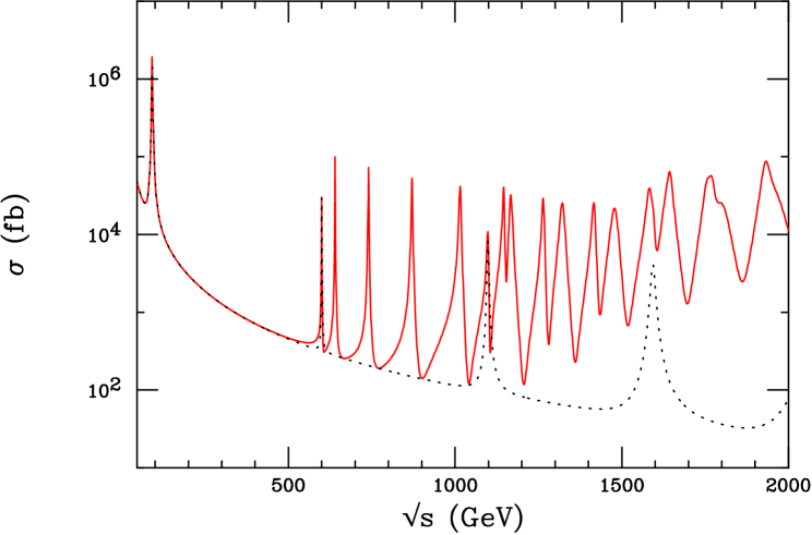
Figure 6: The solid red curve corresponds to the cross section for $e^{+}e^{-}\rightarrow\mu^{+}\mu^{-}$ when the additional dimension is not orbifolded, i.e., for the case of $S^{1}$, with $m_{10}=600$ GeV, $k/\overline{M}_{Pl}=0.03$ and $kR=1$. The result for the conventional RS model is also displayed, corresponding to the dotted curve.

2.4 Placing the Standard Model Fields in the $S^{1}/Z_{2}$

We now discuss the scenario where the SM fields are allowed to propagate in the additional orbifolded $S^{1}/Z_{2}$ dimension. Note that the orbifold symmetries must be present when the SM is in this manifold in order to remove the extra zero-mode fields which result from the KK expansion of the SM fields. We remind the reader that the placement of the SM fields in the RS bulk is problematic due to the large contribution of the resulting KK states to precision electroweak observables [3]; we thus do not consider this option here.

2.4.1 Constraints from Precision Measurements

We first consider the case of placing only the SM gauge fields in the $S^{1}/Z_{2}$ manifold. In this scenario, the exchange of their KK excitations can give significant contributions to the precision electroweak observables which leads to strong lower bounds on the associated compactification scale [16]. In the present case, this also yields constraints on the graviton KK spectrum since the KK gauge and graviton masses are linked in a very simple way. The masses of the KK gauge excitations are given by $m^{A}_{l}=(l/R)e^{-\pi kr_{c}}$. The first gauge KK state can then be written in terms of the lowest lying graviton KK state as $m^{A}_{1}=m_{10}/kRx_{10}$, implying that $m_{10}\simeq 3.83kRm^{A}_{1}$. Given a constraint on $m^{A}_{1}$ from a global fit to the precision electroweak data, this relationship places a lower bound on the first KK graviton mass as a function of $kR$. This in turn sets a limit on $\Lambda_{\pi}$ since $m_{10}=x_{10}\Lambda_{\pi}k/\overline{M}_{Pl}$. The lower bound on $m^{A}_{1}$ in this scenario is exactly the same as that arising in the more familiar case of TeV-scale flat space theories and is approximately given by 5 TeV[16] when the SM fermions and Higgs fields are confined to the TeV-brane, i.e., the fixed point at $\theta=0$. In this simple case this result implies that $m_{10}\geq 19kR$ TeV and further that

$$\Lambda_{\pi}\geq 100kR{0.05\over{(k/\overline{M}_{Pl})}}\rm{TeV}\,.$$ (27)

This is uncomfortably large for $kR$ near unity and favors smaller values of order $\sim 0.2$ or less, which is not far from the lower end of our natural region.

Of course, confining all the SM fields at the $\theta=0$ fixed point is not the scenario we envision as we want to address the problem of proton decay and other issues through fermion localization[7]. Localization of the SM fermions in the $S^{1}/Z_{2}$ manifold will in general lower the bound of $m^{A}_{1}\simeq 5$ TeV, since the couplings of the SM fermions to the gauge KK states are dependent on their point of localization. These couplings are then proportional to $\cos l\theta_{f}$, where $\theta_{f}$ is the localization point for a given fermion; since the magnitude of this quantity is always less than unity, this implies smaller fermionic KK gauge couplings and thus weaker bounds from the data. An analysis of all precision measurements with arbitrarily localized fermions is beyond the scope of this paper, but to demonstrate this phenomena we consider a toy model in which the SM leptons are all localized at $\theta_{l}=\pi z_{l}$ and the quarks are elsewhere. As is well known, most of the constraints set from precision measurements arise from fits to the observables $M_{W}$ and $\sin^{2}\theta_{eff}$, where the latter essentially determines the leptonic coupling at the $Z$-pole. These observables depend on $z_{l}$ and are independent of the location of the quark fields and hence we can examine the fraction by which the 5 TeV bound softens as we vary $z_{l}$ away from zero. The results of this simple analysis are shown in Fig. 7. Here we see that within this toy model the bound can be softened by as much as $50\%$. Based on this short analysis one might expect that in a more realistic situation with all the fermions localized in various places in the $S^{1}/Z_{2}$ it may be possible to reduce this constraint even further, perhaps to the 1-2 TeV range. If this were so, then values of $kR$ as large as unity would be acceptable without having to invoke fine-tuning.

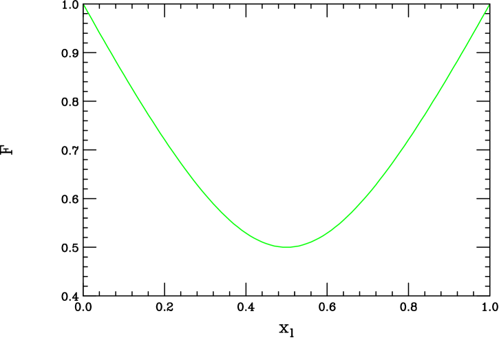
Figure 7: Fractional softening of the $\simeq 5$ TeV lower bound on the lightest gauge boson KK mass as a function of the location of the SM leptons in the $S^{1}/Z_{2}$ manifold for the toy model discussed in the text.

2.4.2 Flavor Changing Graviton KK Interactions

We now discuss other effects from localizing the SM fermions at various points along the $S^{1}/Z_{2}$ dimension. Fermion localization may be achieved by the use of a kink solution of a varying domain wall scalar [7]; the fermions then obtain narrow Gaussian-like wavefunctions with a width much smaller than the compactification scale for this dimension. The $l=0$ graviton KK states have a flat wavefunction along this dimension and hence are not sensitive to the fermion locations. However, the wavefunction for the $l\neq 0$ graviton KK states goes as $\sim\cos l\theta$ and thus these states will have different overlaps with fermions placed at distinct points. In particular, flavor changing (FC) couplings for these graviton KK states will result if the fermion generations are localized at different spots. Similar FC effects for gauge KK states have been studied [17] in the case where the SM fields are located in an TeV^-1 extra dimension. We also point out that FC graviton KK interactions may be present [18] in conventional RS models when the SM fermions propagate in the warped geometry.

Such FC graviton KK couplings are induced by fermion mixing. The overlap of the wavefunction for an $l\neq 0$ graviton KK state with a left-handed fermion of type $i$ localized at the point $\theta=\theta_{i}$ is given by

$$x^{i}_{L}=\int d\theta\bar{f}_{L,i}(\theta)f_{L,i}(\theta)\phi^{l}(\theta)\,,$$ (28)

where $f_{i}(\theta)$ is a gaussian of width $\sigma$, $\exp(-\lambda(\theta-\theta^{i}_{L})^{2}/2\sigma^{2})$, and similarly for the right-handed fermions. Approximating the fermion gaussian wavefunctions by a delta-function, $\delta(\theta-\theta^{i})$, gives $x^{i}_{L,R}=\cos l\theta^{i}_{L,R}$. The 4-dimensional interaction Lagrangian for an $(n,l)$ graviton KK state is then

$${\cal L}_{int}={-1\over\Lambda_{\pi}}\sum_{i}(\bar{f}^{0}_{L,i}\tilde{T}^{\mu\nu}x^{i}_{L}f^{0}_{L,i}+\bar{f}^{0}_{R,i}\tilde{T}^{\mu\nu}x^{i}_{R}f^{0}_{R,i})\xi(n,l)h^{(n,l)}_{\mu\nu}\,$$ (29)

in the fermion weak eigenstate basis, and where we have written the stress-energy tensor as $T^{\mu\nu}=\bar{f}\tilde{T}^{\mu\nu}f$. In the fermion mass eigenstate basis, this becomes

$${\cal L}_{int}={-1\over\Lambda_{\pi}}\sum_{i}(\bar{f}_{L,i}\tilde{T}^{\mu\nu}U_{L}x^{i}_{L}(U_{L})^{\dagger}f_{L,i}+\bar{f}_{R,i}\tilde{T}^{\mu\nu}U_{R}x^{i}_{R}(U_{R})^{\dagger}f_{R,i})\xi(n,l)h^{(n,l)}_{\mu\nu}\,,$$ (30)

where $U_{L,R}$ represent the bi-unitary transformations which diagonalize the fermion fields, i.e., $M^{Diag}=U_{L}^{\dagger}m^{0}U_{R}$. We denote the mixing factors which induce FC interactions for the graviton KK states as

$$X_{L,R}=U^{\dagger}_{L,R}\left(\begin{array}[]{ccc}x^{d}&0&0\\ 0&x^{s}&0\\ 0&0&x^{b}\end{array}\right)U_{L,R}\,,$$ (31)

which gives, for example, $X^{ij}_{L}=(U^{\dagger}_{L})_{ik}x^{k}_{L}\delta_{ak}(U_{L})_{aj}$.

These couplings can induce flavor changing neutral current (FCNC) reactions which are mediated by tree-level graviton KK exchange. These in principle could occur at a sizeable level and pose a threat to this scenario. For purposes of demonstration, we examine the process $B_{q}\rightarrow\ell^{+}\ell^{-}$ (where $q=d$ or $s$) in order to provide an estimate of the magnitude of such effects. In this case, using the Feynman rules of Ref. [9], the amplitude for the tree-level graviton KK contribution to this decay is given by

$${\cal A}={2\over\Lambda_{\pi}^{2}}\sum_{l=1}^{\infty}\sum_{n=1}^{\infty}\xi(n,l)^{2}(\bar{q}\tilde{T}^{\mu\nu}b)(\bar{\ell}\tilde{T}^{\alpha\beta}\ell){P_{\mu\nu\alpha\beta}\over k^{2}-m^{2}_{nl}}\,,$$ (32)

where $P_{\mu\nu\alpha\beta}$ is the spin-sum of the graviton KK polarization tensors, $\xi(n,l)$ is defined in Eq. (22), and $k$ represents the momentum transfer to the final state which can be neglected in comparison to the graviton KK masses. Here, we have suppressed the mixing factors; their contributions will be explicitly determined below.

In order to compute the rate, we must determine the matrix element of the hadronic current

$$\langle 0\,|\,\bar{q}\tilde{T}^{\mu\nu}b\,|\,B\rangle\,,$$ (33)

where the appearance of the stress-energy tensor leads to the factor $i[(p_{b}-p_{q})^{\mu}\gamma^{\nu}+(p_{b}-p_{q})^{\nu}\gamma^{\mu}]/4$, with $p_{i}$ being the momenta of the $i^{th}$ quark inside the $B$ meson. We make use of Heavy Quark Effective Theory [19] in the evaluation of this matrix element, which yields

$${i\over 4}\langle 0\,|\,\bar{q}[p_{B}^{\mu}\gamma^{\nu}+p_{B}^{\nu}\gamma^{\mu}]b\,|\,B\rangle\,,$$ (34)

where we have neglected terms of order $\Lambda_{QCD}/m_{B}$. Due to parity considerations, only axial-vector contributions yield a non-zero value for this matrix element. These are realized in the present scenario in the case where the left- and right-handed fermions of a given flavor are localized at separate points. Indeed, such a configuration could generate the flavor hierarchy by giving the wavefunctions of the left- and right-handed fields different degrees of overlap in the $S^{1}/Z_{2}$ dimension [7]. Using the familiar result

$$\langle 0\,|\,\bar{q}\gamma^{\mu}\gamma_{5}b\,|\,B\rangle=-if_{B}p_{B}^{\mu}\,,$$ (35)

we then find

$$\langle 0\,|\,\bar{q}\tilde{T}^{\mu\nu}b\,|\,B\rangle={-f_{B}\over 2}(X^{qb}_{L}-X^{qb}_{R})p_{B}^{\mu}p_{B}^{\nu}\,,$$ (36)

where $f_{B}$ is the decay constant of the $B$ meson and the mixing factors are defined above. We see that this matrix element indeed vanishes when the left- and right-handed fields are not separated.

Using these results and inserting the form of the polarization sum [9], we find for the square of the amplitude

$$|\langle 0\,|\,{\cal A}\,|\,B\rangle|^{2}={f_{B}^{2}m_{B}^{6}m_{\ell}^{2}\over 2\Lambda_{\pi}^{4}}\Bigg{|}\sum_{l=1}^{\infty}\sum_{n=1}^{\infty}{\xi(n,l)^{2}[X^{qb}_{L}-X^{qb}_{R}][x^{\ell}_{L}-x^{\ell}_{R}]\over m^{2}_{nl}}\Bigg{|}^{2}\,,$$ (37)

which leads to the partial decay width for this contribution

$$\Gamma(B_{q}\rightarrow\ell^{+}\ell^{-})_{grav}={f_{B}^{2}m_{B}^{5}m_{\ell}^{2}\over 32\pi\Lambda^{4}_{\pi}m^{4}_{10}}\bigg{[}1-{4m^{2}_{\ell}\over m_{B}^{2}}\bigg{]}^{1/2}\Bigg{|}\sum_{l=1}^{\infty}\sum_{n=1}^{\infty}{\xi(n,l)^{2}x_{10}^{2}[X^{qb}_{L}-X^{qb}_{R}][x^{\ell}_{L}-x^{\ell}_{R}]\over x^{2}_{nl}}\Bigg{|}^{2}\,.$$ (38)

The overall factor of $m_{\ell}^{2}$ arises from helicity suppression. Here, $x_{nl}$ are the roots which determine the graviton KK masses as discussed above. A numerical evaluation of this width for the case of $B_{s}\rightarrow\mu^{+}\mu^{-}$, with $m_{10}=600$ GeV and $k/\overline{M}_{Pl}=0.1$, yields the result

$$\Gamma(B_{s}\rightarrow\mu^{+}\mu^{-})_{grav}=(2.83\times 10^{-23}{\rm MeV})\Bigg{|}\sum_{l=1}^{\infty}\sum_{n=1}^{\infty}{\xi(n,l)^{2}x_{10}^{2}[X^{qb}_{L}-X^{qb}_{R}][x^{\ell}_{L}-x^{\ell}_{R}]\over x^{2}_{nl}}\Bigg{|}^{2}\,.$$ (39)

In order to estimate the size of the mixing factors, we assume $x^{s}_{L,R}=x^{d}_{L,R}$ and make use of unitarity which yields

$$X^{sb}_{L,R}=(x^{b}_{L,R}-x^{s}_{L,R})(U^{\dagger}_{L,R})_{sb}(U_{L,R})_{bb}\,.$$ (40)

Taking the most optimistic case with the left-(right-)handed fermions being located at $\theta_{l}=0\,(\pi)$, and setting $(U^{\dagger}_{L,R})_{sb}(U_{L,R})_{bb}=\lambda^{3}$ where $\lambda$ represents the Cabbibo mixing angle, we find the graviton KK contribution to the branching ratio for this decay to be

$$BR(B_{s}\rightarrow\mu^{+}\mu^{-})_{grav}\sim 10^{-16}$$ (41)

at the most. Compared to the SM branching fraction of $\sim 10^{-9}$, we see that the KK graviton contributions are safely below the SM prediction. We thus conclude that low-energy FCNC do not pose a dangerous threat to this scenario.

In addition, these flavor changing KK graviton couplings may be observed in the decays of the $n\geq 3$ graviton states at colliders, i.e., $G^{(nl)}\rightarrow t\bar{c}$. Such FC graviton decays have been discussed in [18].

3 The Graviton KK Spectrum and Couplings: Curved Manifolds

Here, we find that for $S^{\delta}$ with $\delta>1$ a new feature arises due to the positive curvature of the $S^{\delta}$. As we will see below, this curvature contributes the same way as a negative cosmological constant to the effective 5-d RS geometry. Thus, it is possible to set the cosmological constant in the non-spherical dimensions to zero and still generate a warped geometry. This fixes the relation between $k$ and $R$ to a value which is within our natural range, thus reducing the number of free parameters, and yields a warp factor that is set geometrically by the radius of the $S^{\delta}$.

To demonstrate the effects of higher dimensional spheres, we will present the relevant formulae for the case of $S^{2}$. The geometries with $\delta>2$ are generalizations of the $\delta=2$ scenario and we briefly comment on them at the end of this section. A simple curved manifold such as $S^{\delta}$ could in principle address proton decay and other model building issues, however the mechanism for localizing fermions on a curved manifold has not yet been demonstrated.

3.1 Formalism

For $\delta=2$, we parameterize the metric as

$$ds^{2}=e^{-2\sigma}\eta_{\mu\nu}dx^{\mu}dx^{\nu}+r_{c}^{2}\,d\phi^{2}+R^{2}(d\theta^{2}+\sin^{2}\theta\,d\omega^{2}),$$ (42)

where we now have $\theta\in[0,\pi]$ and $\omega\in[0,2\pi]$. The cosmological constant and energy-momentum tensors now have the general forms

$$\Lambda^{A}_{B}={\rm diag}(\Lambda,\Lambda,\Lambda,\Lambda,\Lambda,\Lambda_{\theta},\Lambda_{\omega}),$$ (43)

and

$$T^{M}_{N}=-\left\{\delta(\phi)\left(\begin{array}[]{cccc}V^{h}\delta^{\mu}_{\nu}&0&0&0\cr 0&0&0&0\cr 0&0&V_{\theta}^{h}&0\cr 0&0&0&V_{\omega}^{h}\end{array}\right)+\delta(\phi-\pi)\left(\begin{array}[]{cccc}V^{v}\delta^{\mu}_{\nu}&0&0&0\cr 0&0&0&0\cr 0&0&V_{\theta}^{v}&0\cr 0&0&0&V_{\omega}^{v}\end{array}\right)\right\},$$ (44)

respectively.

As before, using the metric in (42) and solving Einstein’s equations component by component, will fix the various parameters of the model. For example, the $(4,4)$ component yields the following for the warping scale

$$k^{2}=\frac{-\Lambda}{24M_{F}^{5}}+\frac{1}{6R^{2}}.$$ (45)

Here, we explicitly see that the curvature of the sphere contributes to the scale $k$ in the same fashion as a negative cosmological constant. The other non-trivial components of Einstein’s equation yield the following relations

$$V^{h}=-V^{v}=24\,M_{F}^{5}\,k\,\,\,;\,\,\,V_{\omega}^{i}=V_{\theta}^{i}=\frac{4}{3}V^{i},$$ (46)

where $i=h,v$ and

$$\Lambda_{\omega}=\Lambda_{\theta}=\frac{5\Lambda}{3}-\frac{20}{3R^{2}}M_{F}^{5}.$$ (47)

Eqs.(45), (46), and (47) show that we now have the freedom to choose $\Lambda$ to be zero, or even positive, as long as $k^{2}>0$. In particular, for $\Lambda=0$ we obtain uniquely the relation $k=1/(\sqrt{6}R)$ which lies in our natural range of values for $kR$. In this case, the warped geometry in the RS model arises solely from the curvature of the $S^{2}$ manifold.

The relation between $\overline{M}_{Pl}$ and $M_{F}$ is now given by

$$\overline{M}_{Pl}^{2}=\frac{4\pi R^{2}}{k}\,M_{F}^{5}[1-e^{-2\sigma(\pi)}].$$ (48)

We again focus on metric perturbations of the form in (8). Here, due to the spherical symmetry of $S^{2}$, we choose the following KK expansion for the graviton

$$h_{\mu\nu}(x,\phi,\theta,\omega)=\sum_{n,l,m}h^{(n,\,l,\,m)}_{\mu\nu}(x)\frac{\chi^{(n,\,l)}(\phi)}{\sqrt{r_{c}}}\frac{Y^{m}_{l}(\theta,\omega)}{R},$$ (49)

where the $Y^{m}_{l}(\theta,\omega)$ are the spherical harmonics. The above expansion yields an equation of motion which is similar to that obtained for the case with $\delta=1$. We have

$$-\frac{1}{r_{c}^{2}}\frac{d}{d\phi}\left(e^{-4\sigma}\frac{d}{d\phi}\chi^{(n,\,l)}(\phi)\right)+e^{-4\sigma}\,\frac{l(l+1)}{R^{2}}\,\chi^{(n,\,l)}(\phi)=e^{-2\sigma}m_{nl}^{2}\chi^{(n,\,l)}(\phi).$$ (50)

The solution for $\chi^{(n,\,l)}$ is given in (13), where we now have

$$\nu\equiv\sqrt{4+\frac{l(l+1)}{(kR)^{2}}}\,.$$ (51)

Substituting the definition (51) for $\nu$ in Eqs.(15) and (16) we obtain the normalization coefficients $N_{nl}$ and the roots $x_{nl}$ which determine the masses $m_{nl}$ as before.

We are now in a position to derive the coupling of the graviton KK tower to the 4-d localized fields. By spherical symmetry we may choose any point on the sphere to place the 4-d fields. A particularly convenient choice is $\theta=0$, for which we have

$$Y^{m}_{l}(0,\omega)=\sqrt{\frac{2l+1}{4\pi}}\delta_{m,0}\,\,.$$ (52)

This demonstrates that, at this point, the coupling is independent of $\omega$ and that for any $l$ only the $m=0$ states couple. For the case when the 4-d fields are localized at $\theta=\pi$, the above is modified by the overall factor $(-1)^{l}$.

The coupling of the 7-d graviton to the 4-d energy-momentum tensor is given by

$${\cal L}=-\frac{1}{M_{F}^{5/2}}h^{\mu\nu}(x,\pi,0,\omega)T_{\mu\nu}(x).$$ (53)

Using the solutions to (50), Eq.(52), and substituting the KK expansion (49) in the above, we obtain

$${\cal L}=-\frac{1}{\overline{M}_{Pl}}h_{\mu\nu}^{(0,\,0,\,0)}(x)T^{\mu\nu}(x)-\frac{1}{\Lambda_{\pi}}T^{\mu\nu}(x)\sum_{l=0}^{\infty}\sum_{n=1}^{\infty}\eta(n,l)h_{\mu\nu}^{(n,\,l,\,0)}(x),$$ (54)

where

$$\eta(n,l)=\sqrt{2l+1}\left[1-\frac{l(l+1)}{(kRx_{nl})^{2}}\right]^{-1/2}.$$ (55)

As in the case of the $S^{1}$ and $S^{1}/Z_{2}$ manifolds, we see that only warped graviton KK states exist (i.e., there are no $\chi^{(n,l)}=$ constant modes for $l\neq 0$).

3.2 Numerical Results

We first display the resulting KK spectrum from this analysis for the case of $S^{2}$ in Fig. 8. Compared to the case with $\delta=1$, we now have more KK states, however the number of states which couple to the 4-d fields is the same; the strength of this coupling is now stronger. From the figure, we see that the first few resonances are clearly observable, whereas the higher resonances are blurred. In this case, we see that the sharp rise in the cross section results in an early onset of unitarity violation, and hence the model parameters in this case are restricted.

As a last possibility, we briefly discuss the extension of $S^{2}$ to the case $S^{p}$, where $2<p\leq 5$. Although we have not explicitly performed a detailed derivation of the resulting KK expansion and couplings to the 4-d fields in this higher dimensional case, we can make use of the work of [20] to anticipate how this generalization might proceed. We consider the case where all SM fields are constrained to the fixed point, which corresponds to $\theta=0$ for arbitrary $p$. (In addition to $\theta$ there will also be $p-1$ azimuthal-like co-ordinates $\phi_{i}$.) We only consider how the masses, couplings and degeneracies of the KK states might be altered for arbitrary $p$. Comparing to the case of $S^{1}$, the results of [20] suggest that the terms proportional to $l^{2}$ in both the expressions for $\nu$ and $\xi$ are given by the eigenvalues of the square of the angular momentum operator. Generalizing to a $p$-sphere, we would have $l^{2}\rightarrow L^{2}\rightarrow l(l+p-1)$. We assume that the KK excitations with non-trivial azimuthal quantum numbers will not couple to the SM fields at the fixed point. This implies that although each $l$ level is multiply degenerate, only one of these graviton KK states will couple to the SM fields. In addition, we assume that the overall couplings pick up an additional factor due to the normalization of the angular wavefunctions which can be determined for any value of $p$ [20]. We note that each of these modifications are verified in the case of $S^{2}$ by our preceding analysis.

Fig. 8 also displays our results for the KK spectrum in the case of an $S^{5}$ manifold, making use of our assumptions listed above regarding the generalization to higher dimensional spheres. With the above assumed modifications, we see that the individual KK states become somewhat less distinct in higher dimensional spherical geometries. Note also that the mass of the $n=l=1$ resonance tends to increase as the dimensionality of the sphere grows.

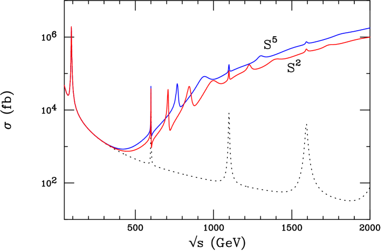
Figure 8: The cross section for $e^{+}e^{-}\rightarrow\mu^{+}\mu^{-}$ when the additional dimension is curved with $m_{10}=600$ GeV, $k/\overline{M}_{Pl}=0.03$ and $kR=1$. The lower solid (red) curve corresponds to the manifold $S^{2}$, while the upper solid (blue) curve represents the case $S^{5}$. The result for the conventional RS model is also displayed, corresponding to the dotted curve.

4 Conclusions

The RS model offers a natural 5-d mechanism for generating the gauge hierarchy. However, it leaves a number of questions, such as proton decay, flavor, and the nature of quantum gravity, unanswered. Whether from a model building point of view, or from a more fundamental standpoint, it may be necessary to embed the RS scenario in a higher dimensional space to address such questions.

In this paper, we assumed that the RS model is endowed with $\delta\geq 1$ additional dimensions compactified on a manifold ${\cal M}^{\delta}$. The background geometry was taken to be of the form $|AdS_{5}|\times{\cal M}^{\delta}$, a direct product of the original RS geometry and ${\cal M}^{\delta}$. We considered two classes of manifolds: flat and curved. We then studied the parameters required to establish these backgrounds, as well as the resulting graviton KK spectrum, couplings, and the corresponding collider phenomenology. For simplicity, we chose ${\cal M}^{\delta}=S^{\delta}$. In the case of flat geometries, we studied $S^{1}/Z_{2}$ and $S^{1}$ as simple representative manifolds. The $S^{1}/Z_{2}$ case is of particular interest, since the fermion localization mechanism on this space has been studied in detail [7] and can address questions of proton stability and flavor, in a simple geometric way. We analyze the collider spectroscopy of this model and find that a forest of new KK graviton states, in addition to the original RS modes, appear at the weak scale. This is a generic signature of the models that we study. The new modes originate from the ‘angular’ graviton excitations over $S^{\delta}$.

The size $R$ of the radius of the $S^{1}$, in units of the inverse 5-d curvature scale $k$, is of key importance and sets the scales of mass and separation of the KK modes. We also find that for $kR\sim 1$, the couplings of different light KK modes to the 4-d SM fields are measurably non-universal. This is in contrast to the 5-d RS model where such non-universality was exponentially suppressed. If the SM fields reside in the $S^{1}/Z_{2}$ extra dimension, the couplings of various localized fermions to a particular KK state of the graviton or gauge fields would be non-universal, and we expect tree-level FCNC effects to arise in KK mediated processes. We have checked that the size of such FCNC effects do not occur at a dangerous level in this scenario. We also show that over the natural range of parameters in this model, observable experimental signatures can be expected at the LHC or a future $e^{+}e^{-}$ collider.

In the case of curved manifolds, we studied $S^{2}$ as an example. Here, a new feature arises which is the possibility of using the positive curvature of $S^{2}$ in order to generate a negative 5-d cosmological constant $\Lambda$. This allows us to choose $\Lambda=0$ along the original 5-d spacetime of the RS model and generate the required warping of $AdS_{5}$ from the curvature of the $S^{2}$. This fixes all the parameters of the model in terms of only three quantities: the fundamental scale $M_{F}$, the size of the $AdS_{5}$ slice $r_{c}$, and the radius $R$ of $S^{2}$. We note that positive values of 5-d $\Lambda$ are also allowed, as long as $k^{2}>0$. In going from $S^{1}$ to $S^{2}$ the collider phenomenology does not change significantly. However, the angular KK states get more strongly coupled with growing mass, resulting in wider KK resonances with more overlap. This has the effect of smearing the spectrum.

Although we only studied $S^{1}/Z_{2}$, $S^{1}$, and $S^{2}$, generalization to $S^{\delta}$, $\delta>2$, is straightforward. We comment on the expected behavior, using $S^{5}$ as an example, without a detailed analysis. A simple modification of our results for $S^{2}$ suggests that compactifying on $S^{5}$ does not change the collider phenomenology significantly. Future directions for expanding our work include incorporating the effects of KK self-couplings as well as gravi-scalar and gravi-vector interactions (present for $d>5$), and investigating the possibility of obtaining new warped 5-d effective theories from different choices of ${\cal M}^{\delta}$.

Acknowledgements

The authors would like to thank Tim Barklow, Tony Gherghetta, Juan Maldacena, and Massimo Porrati for discussions related to this work. The work of H.D. was supported by the US Department of Energy under contract DE-FG02-90ER40542.

References

- [1] L. Randall and R. Sundrum, Phys. Rev. Lett. 83, 3370 (1999) [arXiv:hep-ph/9905221], and Phys. Rev. Lett. 83, 4690 (1999) [arXiv:hep-th/9906064].
- [2] H. Davoudiasl, J. L. Hewett and T. G. Rizzo, Phys. Rev. Lett. 84, 2080 (2000) [arXiv:hep-ph/9909255].
- [3] H. Davoudiasl, J. L. Hewett and T. G. Rizzo, Phys. Rev. D 63, 075004 (2001) [arXiv:hep-ph/0006041] and Phys. Lett. B 473, 43 (2000) [arXiv:hep-ph/9911262]; A. Pomarol, Phys. Lett. B 486, 153 (2000)[arXiv:hep-ph/9911294]; T. Gherghetta and A. Pomarol, Nucl. Phys. B 586, 141 (2000); S. Chang, J. Hisano, H. Nakano, N. Okada and M. Yamaguchi, Phys. Rev. D 62, 084025 (2000)[arXiv:hep-ph/9912498]; R. Kitano, Phys. Lett. B 481, 39 (2000)[arXiv:hep-ph/0002279]; S. J. Huber and Q. Shafi, Phys. Lett. B 498, 256 (2001) [arXiv:hep-ph/0010195] and Phys. Rev. D 63, 045010 (2001) [arXiv:hep-ph/0005286]; S. J. Huber, C. A. Lee and Q. Shafi, arXiv:hep-ph/0111465; J. L. Hewett, F. J. Petriello and T. G. Rizzo, JHEP 0209, 030 (2002) [arXiv:hep-ph/0203091]; F. Del Aguila and J. Santiago, arXiv:hep-ph/0111047, arXiv:hep-ph/0011143, Nucl. Phys. Proc. Suppl. 89, 43 (2000)[arXiv:hep-ph/0011142] and Phys. Lett. B 493, 175 (2000)[arXiv:hep-ph/0008143]; C. S. Kim, J. D. Kim and J. Song, arXiv:hep-ph/0204002.
- [4] K. R. Dienes, E. Dudas and T. Gherghetta, Phys. Lett. B 436, 55 (1998) [arXiv:hep-ph/9803466]; Nucl. Phys. B 537, 47 (1999) [arXiv:hep-ph/9806292]; Nucl. Phys. B 567, 111 (2000) [arXiv:hep-ph/9908530]; L. Randall and M. D. Schwartz, Phys. Rev. Lett. 88, 081801 (2002) [arXiv:hep-th/0108115], and JHEP 0111, 003 (2001) [arXiv:hep-th/0108114]; W. D. Goldberger and I. Z. Rothstein, arXiv:hep-th/0208060; W. D. Goldberger, Y. Nomura and D. R. Smith, arXiv:hep-ph/0209158.
- [5] I. Antoniadis, Phys. Lett. B 246, 377 (1990); D. E. Kaplan, G. D. Kribs and M. Schmaltz, Phys. Rev. D 62, 035010 (2000) [arXiv:hep-ph/9911293], Z. Chacko, M. A. Luty, A. E. Nelson and E. Ponton, JHEP 0001, 003 (2000) [arXiv:hep-ph/9911323]; N. Arkani-Hamed, L. J. Hall, D. R. Smith and N. Weiner, Phys. Rev. D 63, 056003 (2001) [arXiv:hep-ph/9911421].
- [6] Y. Grossman and M. Neubert, Phys. Lett. B 474, 361 (2000) [arXiv:hep-ph/9912408]; K. R. Dienes, E. Dudas and T. Gherghetta, Nucl. Phys. B 557, 25 (1999) [arXiv:hep-ph/9811428]; N. Arkani-Hamed, S. Dimopoulos, G. R. Dvali and J. March-Russell, Phys. Rev. D 65, 024032 (2002) [arXiv:hep-ph/9811448].
- [7] N. Arkani-Hamed and M. Schmaltz, Phys. Rev. D 61, 033005 (2000) [arXiv:hep-ph/9903417].
- [8] C. Csaki, J. Erlich, T. J. Hollowood and Y. Shirman, Nucl. Phys. B 581, 309 (2000) [arXiv:hep-th/0001033]; T. Gherghetta and M. E. Shaposhnikov, Phys. Rev. Lett. 85, 240 (2000) [arXiv:hep-th/0004014].
- [9] G. F. Giudice, R. Rattazzi and J. D. Wells, Nucl. Phys. B 544, 3 (1999) [arXiv:hep-ph/9811291]; T. Han, J. D. Lykken and R. J. Zhang, Phys. Rev. D 59, 105006 (1999) [arXiv:hep-ph/9811350].
- [10] I. I. Kogan, S. Mouslopoulos, A. Papazoglou and G. G. Ross, Phys. Rev. D 64, 124014 (2001) [arXiv:hep-th/0107086]; T. Multamaki and I. Vilja, arXiv:hep-th/0207263.
- [11] W. D. Goldberger and M. B. Wise, Phys. Rev. D 60, 107505 (1999) [arXiv:hep-ph/9907218].
- [12] K. R. Dienes, Phys. Rev. Lett. 88, 011601 (2002) [arXiv:hep-ph/0108115].
- [13] H. Davoudiasl and T. G. Rizzo, Phys. Lett. B 512, 100 (2001) [arXiv:hep-ph/0104199].
- [14] M. Battaglia, A. De Roeck and T. Rizzo, in Proc. of the APS/DPF/DPB Summer Study on the Future of Particle Physics (Snowmass 2001) ed. N. Graf, arXiv:hep-ph/0112169.
- [15] “ATLAS detector and physics performance. Technical design report. Vols. 1 and 2,”CERN-LHCC-99-14 and 99-15.
- [16] See, for example, T. G. Rizzo and J. D. Wells, Phys. Rev. D 61, 016007 (2000) [arXiv:hep-ph/9906234]; M. Masip and A. Pomarol, Phys. Rev. D 60, 096005 (1999) [arXiv:hep-ph/9902467]; T. G. Rizzo, Phys. Rev. D 64, 015003 (2001) [arXiv:hep-ph/0101278]; A. Muck, A. Pilaftsis and R. Ruckl, arXiv:hep-ph/0203032 and Phys. Rev. D 65, 085037 (2002)[arXiv:hep-ph/0110391]; K. m. Cheung and G. Landsberg, Phys. Rev. D 65, 076003 (2002) [arXiv:hep-ph/0110346] and references therein; C. D. Carone, Phys. Rev. D 61, 015008 (2000) [arXiv:hep-ph/9907362]; A. Strumia, Phys. Lett. B 466, 107 (1999) [arXiv:hep-ph/9906266]; R. Casalbuoni, S. De Curtis, D. Dominici and R. Gatto, Phys. Lett. B 462, 48 (1999) [arXiv:hep-ph/9907355].
- [17] A. Delgado, A. Pomarol and M. Quiros, JHEP 0001, 030 (2000) [arXiv:hep-ph/9911252].
- [18] H. Davoudiasl and T. G. Rizzo, Phys. Lett. B 512, 100 (2001) [arXiv:hep-ph/0104199].
- [19] For a review of Heavy Quark Effective Theory, see, M. Neubert, Phys. Rept. 245, 259 (1994) [arXiv:hep-ph/9306320].
- [20] A. Kehagias and K. Sfetsos, Phys. Lett. B 472, 39 (2000) [arXiv:hep-ph/9905417]; F. Leblond, Phys. Rev. D 64, 045016 (2001) [arXiv:hep-ph/0104273].