Radion Induced Baryogenesis

Abstract

Recent work in two brane Randall-Sundrum models has shown that the radion can drive parametric amplification of particles on the TeV brane leading to a stage of cosmology similar to preheating. We consider radion induced preheating as a mechanism for electroweak scale baryogenesis and estimate the baryon to entropy ratio for some regions of parameter space. We also predict an upper bound for the radion mass, which makes this baryogenesis mechanism testable. Finally, we verify some assumptions with numerical calculations of the 1+1 dimensional Abelian Higgs model.

I Introduction

The high degree of symmetry between matter and anti-matter in our theories has long seemed in contradiction with the overwhelming presence of matter (baryons) around us. Electroweak baryogenesis reviews provides a testable explanation of the baryons within the context of the standard models of particle physics and cosmology but suffers from the two difficulties of providing enough CP violation and providing enough departure from equilibrium. In the usual picture transitions between vacua of the electroweak theory correspond, via an anomaly, to changes in baryon plus lepton number. If the electroweak phase transition in the early universe is strongly first order then the presence of CP violation will cause sphaleron transitions near bubble walls to favor formation of matter over anti-matter. While the minimal supersymmetric standard model may provide the first order phase transition and CP violation needed for this picture of baryogenesis, a radically different picture is possible within the context of the Randall-Sundrum model.

As with supersymmetry, the two-brane Randall-Sundrum model rsa (RS) provides a framework for addressing the hierarchy problem. The model consists of a slice of five dimensional anti-de Sitter space ($AdS_{5}$) truncated by two 3-branes with the standard model particles trapped on one of the branes. The gravitational warping between the branes generates hierarchies of mass scales. With the stabilization of the brane separation provided by Goldberger and Wise gw , mass scales are naturally stabilized providing a solution to the hierarchy problem along with an acceptable low-energy phenomenology. The separation between the branes corresponds to a particle called the radion which is expected to be the lightest new degree of freedom.

Initially, it might seem difficult to explain the baryon asymmetry within the context of RS since RS physics becomes important just above the electroweak scale. For example, it is not possible to use existing extensions of standard model physics to explain baryogenesis within an effective theory that integrates out RS physics. They are at the same scale. We must, therefore, re-examine the baryogenesis question within the context of the RS model. Fortunately, the radion provides a new route for departure from equilibrium; previous work has shown that homogeneous oscillations of the radion lead to exponential growth of scalar particles on the standard model brane radion_preheating . The produced particles do not have a thermal distribution, but lie in a small region of momentum space. These are features common to parametric amplification, or preheating inflation_preheating , as it occurs in the inflationary context.

We use parametric amplification of the standard model Higgs field to drive the field over the potential barrier, allowing for the creation of winding modes and, consequently vacuum transitions. This parametric amplification, rather than bubbles from a first order phase transition, generates the departure from equilibrium. With an additional source of CP violation, the decay of the Higgs windings will favor the production of baryons over anti-baryons. However, there are constraints on the mass of the radion coming from the size of windings which give rise to baryon number violating transitions. Generically, if the radion is too massive, then the parametric amplification gives windings which are too small for baryogenesis. The radion should not be much more massive than three times the mass of the Higgs boson. Furthermore, because the radion is a gravitational mode in the full theory, the form of the radion-Higgs coupling is determined with only one free parameter (we consider only minimal coupling of the Higgs).

The next sections review relevant aspects of the standard model baryon violation and the RS model. We then discuss radion induced preheating and consequences for baryogenesis. We explain some constraints on the model and estimate the baryon asymmetry for a simple case. The final section shows numerical results which verify some assumptions and help develop our intuition.

II Baryogenesis in the Standard Model

As alluded to above, non-perturbative effects in the electroweak sector of the standard model violate baryon number. An anomaly links the change in baryon and lepton number to the change in Chern-Simons number:

$$\Delta B=\Delta L=n_{f}\Delta N_{CS},$$ (1)

where $n_{f}$ is the number of families of matter fermions. In the absence of fermions the vacua of this theory are degenerate and they are labeled by the winding number of the Higgs field. In any vacuum state the Chern-Simons number is equal to the Higgs winding number. The transition from one vacuum state to another must therefore involve a change in both the Higgs and gauge fields so that both the Higgs winding and the Chern-Simons number remain equal. See the reviews in reviews for more details. This baryon violating transition between vacua passes through a field configuration known as the sphaleron, which is a saddle point of the effective potential. Henceforth, we refer to the sphaleron mediated transitions between vacua as the sphaleron transition.

We can now understand that an initial configuration with the Higgs winding differing from the Chern-Simons number by one unit must relax to a vacuum in one of two ways: either the Higgs winding will change, which does not violate baryon number; or the gauge field evolution will change the Chern-Simons number, which does violate baryon number. The method by which the relaxation occurs is dependent upon the length scale of the winding. In general a Higgs winding will collapse and the time scale for the collapse is simply the length scale turok_zadrozny . However, the gauge fields will evolve to cancel gradient energy in a Higgs winding with time scale loosely set by the gauge boson mass. So a sufficiently small winding will collapse and the Higgs winding number will change, while a sufficiently large winding will be canceled by the gauge field thus changing baryon number.

Some critical length scale separates these two regimes. If there is initially an equal density of windings and anti-windings on large scales and no CP violation, then there will be equal production of baryons and anti-baryons. According to the picture of Turok and Zadrozny turok_zadrozny , CP violation will affect the critical length differently for windings and anti-windings. An anti-winding near the critical scale will preferentially unwind through Higgs field evolution, while a winding at the same scale will unwind by gauge field evolution, thus favoring production of baryons. The critical length is about $3\,m_{W}^{-1}\sim(30\,GeV)^{-1}$ if the gauge boson mass is given by the zero temperature vacuum. The realistic picture is more complicated lrt with the length scale being a function of other parameters which characterize a winding, but there should still be a range of critical length scales separating Higgs field unwinding from baryon number changing.

In the high temperature, symmetry restored vacuum, simple dimensional analysis gives the sphaleron length scale as being the magnetic screening length, $(\alpha_{W}T)^{-1}$, which could be as large as about $(3\,GeV)^{-1}$. For the remainder of the paper we work with the length scale $l_{sph}=(20\,GeV)^{-1}$. We use this length scale to constrain the radion mass since a massive radion will give higher frequency excitations to the Higgs field leading to windings which are too small for baryogenesis.

At temperatures much below the electroweak scale, sphaleron transitions are exponentially suppressed by the energy scale of the potential barrier between electroweak vacua, $E_{sph}\sim 10\,TeV$:

$$\Gamma_{sph}\sim e^{(-E_{sph}/T)}.$$ (2)

For temperatures near the electroweak scale and as low as $150\,GeV$ preheat_lattice , the electroweak symmetry is restored and the sphaleron transitions are unsuppressed. Thermal fluctuations easily form windings of the Higgs or gauge fields and on dimensional grounds

$$\Gamma_{sph}\sim(\alpha_{W}T)^{4}.$$ (3)

It might seem then that a temperature above $150\,GeV$, along with CP violation, is sufficient for the production of baryons. However, the thermal average of baryon number is zero reviews , meaning that baryogenesis must happen during a departure from thermal equilibrium. Furthermore, if equilibrium is restored while sphaleron transitions are unsuppressed, then any existing baryon asymmetry will be destroyed. This process is called thermal washout, and it will constrain the total energy in our model as explained in section IV.

III The Randall-Sundrum Scenario

The background geometry for the two brane Randall-Sundrum model (RS) is given by the metric

$$ds^{2}=e^{-2kz}\eta_{\mu\nu}dx^{\mu}dx^{\nu}+dz^{2},$$ (4)

with branes truncating the space at $z=z_{0}$ and $z=z_{1}$. This geometry is a solution to Einstein’s equations for negative bulk cosmological constant and nonzero brane tensions which scale with $k$. For naturalness $k$ is taken to be near the fundamental Planck scale, $M_{5}$, but somewhat smaller to ensure gravitational perturbativity. The warping of the space red shifts mass scales on the brane at $z_{1}$ relative to the scale at $z_{0}$, allowing for the electroweak theory trapped on the brane at $z_{1}$ to have an energy scale much less than scales on the brane at $z_{0}$. The brane at $z_{1}$ is therefore often called the $TeV$ brane. The separation between the branes corresponds to a modulus known as the radion. By fixing the radion in a natural way, the electroweak hierarchy problem is solved.

The form for the radion which does not mix with the four dimensional graviton cgr is

$$ds^{2} = e^{-2k\left(z+f(x)e^{2kz}\right)}g_{\mu\nu}(x)dx^{\mu}dx^{\nu}$$ (5)

$$+\left(1+2kf(x)e^{2kz}\right)^{2}dz^{2},$$

where $f(x)$ is the radion. Goldberger and Wise gw found that a scalar field in the bulk which has nonzero vacuum expectation values on the branes can naturally determine the brane separation. A competition between the kinetic and potential terms in the five dimensional action for the scalar gives a potential to the radion in the four dimensional effective theory. In other words, after integrating out the bulk degrees of freedom, an effective theory for the radion remains radion_preheating :

$$\mathcal{L}_{F}=-\frac{1}{2}\partial_{\mu}F(x)\partial^{\mu}F(x)-\frac{1}{2}m_{F}^{2}F(x)^{2}+\mathcal{O}(F^{3}).$$ (6)

We have rescaled $f(x)$ to have the properly normalized kinetic term,

$$F(x)=\sqrt{12kM_{5}^{3}}e^{k(z_{1}-z_{0})}f(x)$$ (7)

and the value for the radion mass, $m_{F}$, depends on the details of the bulk scalar. The scale of physics on the $TeV$ brane is set by the parameter $\Lambda=\sqrt{3M_{5}^{3}/k}e^{-k(z_{1}-z_{0})}$. We will only consider small oscillations of the radion, $F(x)\ll\Lambda$, to avoid sensitivity to the higher order terms in the radion effective action.

Now consider a scalar field on the $TeV$ brane. We will see how the warping red shifts mass scales and derive the coupling of the radion to the scalar needed for the next section. We set $z_{0}=0$ for simplicity. The action on the brane is

$$S=-\frac{1}{2}\int d^{4}x\sqrt{-\tilde{g}}\left[\tilde{g}^{\mu\nu}\partial_{\mu}\phi\partial_{\nu}\phi+m^{2}\phi^{2}\right],$$ (8)

with the induced metric on the brane given by

$$ds^{2}=\tilde{g}_{\mu\nu}(x)dx^{\mu}dx^{\nu}=e^{-2k\left(z_{1}+f(x)e^{2kz_{1}}\right)}\eta_{\mu\nu}dx^{\mu}dx^{\nu}.$$ (9)

By rescaling $\phi(x)\rightarrow e^{kz_{1}}\phi(x)$ to give the kinetic term canonical normalization, the action takes the form:

$$S = -\frac{1}{2}\int d^{4}x\,\Bigl{[}e^{-2kf(x)e^{2kz_{1}}}\eta^{\mu\nu}\partial_{\mu}\phi\partial_{\nu}\phi$$ (10)

$$\qquad\qquad\quad+e^{-4kf(x)e^{2kz_{1}}}e^{-2kz_{1}}m^{2}\phi^{2}\Bigr{]}.$$

Notice that the scalar field mass is suppressed by a “warp factor”, $e^{-kz_{1}}$. We define the effective scalar mass $m_{\phi}=e^{-kz_{1}}m$. In terms of the correctly normalized radion, the action is:

$$S = -\frac{1}{2}\int d^{4}x\,\Bigl{[}e^{-F(x)/\Lambda}\eta^{\mu\nu}\partial_{\mu}\phi\partial_{\nu}\phi$$ (11)

$$\qquad\qquad\quad+e^{-2F(x)/\Lambda}m_{\phi}^{2}\phi^{2}\Bigr{]}.$$

This is the action used to study parametric amplification of scalars on the $TeV$ brane radion_preheating . Notice that the universality of gravitational couplings limits the radion-scalar coupling to this form. In the next section we review this parametric amplification and show how baryogenesis occurs.

IV Preheating and Baryogenesis

As we discussed in previous work radion_preheating , there may have been a time in the early universe when most of the energy density was tied up in coherent homogeneous oscillations of the radion. These oscillations might be expected for several reasons. First, an inflation-like mechanism is needed to solve the horizon problem within the RS context, and this mechanism almost certainly will involve physics of the extra dimension. In a minimal model the only way to reheat the $TeV$ brane is through the stabilization mechanism, which would involve oscillations of the stabilizing field and of the radion. We take the potential of the stabilizing field to be stiff and study oscillations of the radion.

Alternatively, at high enough temperatures the space-time is unstable to formation of a bulk horizon, which cuts off the space and removes the $TeV$ brane. As the universe cools, a phase transition occurs rattazzi , generating the $TeV$ brane generically shifted from its equilibrium position. The radion will oscillate coherently as the brane settles in to the equilibrium position. In this scenario we would not expect a cold $TeV$ brane, although more details of this phase transition still need to be understood.

In a third picture, the stabilization mechanism may provide a false vacuum for the radion with the $TeV$ brane at infinitycline . Early universe dynamics could set the brane in this false vacuum with a first order phase transition bringing the brane to the global minimum. Bubbles of the brane in the true vacuum would not be expected to lie exactly at the bottom of the potential, but oscillate around the minimum. In any of these three scenarios, higher energy physics leads to radion oscillations.

We take the radion to be a background of the form

$$F(t)=F_{0}\Lambda\cos(m_{F}t),$$ (12)

and decompose the scalar field in Fourier modes:

$$\phi(t,\vec{x})=\int{d^{3}k\over(2\pi)^{3/2}}\,\left[a_{\vec{k}}\phi_{k}(t)e^{-i\vec{k}\cdot\vec{x}}+a_{\vec{k}}^{\dagger}\phi_{k}^{*}(t)e^{i\vec{k}\cdot\vec{x}}\right].$$ (13)

We then calculate the equation of motion for the scalar modes from the action (11):

$${d^{2}\phi_{k}\over dt^{2}}+F_{0}m_{F}\sin(m_{F}t){d\phi_{k}\over dt}+{\omega}^{2}_{k}(t)\phi_{k}=0,$$ (14)

where ${\omega^{2}_{k}(t)}\equiv\left[|\vec{k}|^{2}+m_{\phi}^{2}e^{-F_{0}\cos(m_{F}t)}\right]$. We start with a vacuum state for all modes,

$${d\phi_{k}\over dt}(0)=-i\omega_{k}(0)\phi_{k}(0),\quad\phi_{k}(0)=\frac{e^{F_{0}/2}}{\sqrt{2\omega_{k}(0)}},$$ (15)

and find exponential growth of some modes. For the specific case $F_{0}=0.5$, the modes unstable to growth are shown in the dark region of figure 1. This is parametric resonance, or preheating.

Figure 1: The instability band for the massive scalar when $F_{0}=0.5$. The dark region shows where there is exponential growth of scalar particles. Both $m_{F}$ and $k=|\vec{k}|$ are expressed in units of the scalar mass.

It should be emphasized that the spectrum of particles produced through parametric amplification is non-thermal and the time scale for growth of particles is given by the radion mass. To show this we calculate the expectation value of the number density operator, $\langle N_{k}(t)\rangle$ (see the appendix for details). In figure 2 we plot $\ln\langle N_{k}(t)\rangle$. The modes in momentum space which grow are those expected by comparing with figure 1. We expect that when backreaction of the scalar on the radion is taken into account, the scalar will drain energy off the radion and damp the amplitude of radion oscillations.

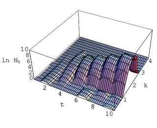
Figure 2: Log of the number density operator, $\ln N_{k}(t)$, for $m_{F}=4m_{\phi}$ and $F_{0}=0.5$. Note that for momenta within the instability band of figure 1, the number of particles produced grows exponentially. All units are appropriate powers of the scalar mass, $m_{\phi}$.

We now want to think about placing the Standard Model on the $TeV$ brane. Again assuming homogeneity and an initial state near the zero temperature vacuum, we would expect Higgs particle production as explained above, where $m_{\phi}$ is now the Higgs mass. Of course, the action for the Higgs field should involve the self-coupling and the coupling to gauge fields. However, leaving these terms out should be a good approximation at the beginning when only the minimum of the potential is being sampled by the Higgs vacuum expectation value. The choice of initial conditions is generalized in the numerical work. We discuss production of fermions and gauge fields below.

The essence of the idea is that the preheating of the Higgs field will produce configurations with winding, in a manner analogous to the production of topological defects following inflationary preheating. These windings will then decay. Some decays will violate baryon number, some will not, and the CP violation will favor production of a small number of net baryons. A similar idea of inflationary preheating leading to baryogenesis has been proposed by others inflate_preheat_baryo1 ; inflate_preheat_baryo2 . However, radion preheating occurs naturally at the proper energy scale, the electroweak scale, and has little freedom in parameter space due to the universality of radion couplings. These concepts are significant: there is no fine tuning needed, as in the inflationary case, to make radion preheating happen at the correct energy scale; and our model will be tested and may be excluded at the next generation of colliders.

IV.1 Constraints

Before estimating the amount of baryogenesis, we would like to discuss some constraints on the radion. First, the final reheat temperature should be sufficiently below the electroweak phase transition to avoid thermal washout of the baryon asymmetry. If, once thermal equilibrium is reached, we require

$$T_{reheat}\lesssim 150\,GeV,$$ (16)

then we must constrain the total energy density:

$$\rho=\frac{\pi^{2}g_{*}}{30}T^{4}\lesssim(350\,GeV)^{4}.$$ (17)

Because the expansion rate of the universe, $H\sim\frac{\sqrt{\rho}}{M_{Pl}}\sim 10^{-15}GeV$, is much less than other relevant scales in the problem, we may ignore the expansion. Then energy conservation restricts the initial radion configuration:

$$\rho_{F}=\frac{1}{2}F_{0}^{2}\Lambda^{2}m_{F}^{2}\lesssim(350\,GeV)^{4}.$$ (18)

Another constraint comes from the location of the instability band. As explained in section II, the length scale for sphaleron configurations, $l_{sph}$, is about $(20\,GeV)^{-1}$. The instability band therefore needs to encompass this value of momentum in order to produce sphaleron configurations. For the case considered in figure 1, this criteria is only satisfied for a radion mass of $1.5\lesssim m_{F}/m_{\phi}\lesssim 3$. More generally, we can understand this constraint by plotting the instability band as a function of $F_{0}$ and $m_{F}$ for fixed $k=l_{sph}^{-1}$ as in figure 3.

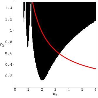
Figure 3: The instability band for the massive scalar when $k=0.16\,m_{\phi}$. This corresponds to $k=l_{sph}^{-1}$ for a Higgs mass of $125\,GeV$. The dark region shows where there is exponential growth of particles. The radion mass is expressed in units of the Higgs mass. Above the line the system contains enough energy to washout baryons after thermalization.

The region above the line is excluded by the energy density constraint. This assumes a Higgs mass of $125\,GeV$, to set a scale, and a fairly low value for the cutoff, $\Lambda=750\,GeV$. These values are used in the remainder of the paper. Equation (18) shows that this line moves down (excluding more of the preheating band) as the lower limit of the cutoff increases or if the Higgs mass becomes heavier. Already we can see that if the radion mass is much above three times the Higgs mass, then there can be no preheating without thermal washout of baryons. For a light radion we need large values of $F_{0}$ for preheating. To trust a calculation in this regime requires knowledge of the complete radion potential. This involves details of the stabilizing mechanism.

While $\mathcal{O}(F^{3})$ and higher terms in the radion action will alter the form of radion oscillations and make a precise large $F_{0}$ calculation of the baryon to entropy ratio difficult, in practice, these terms do not prohibit parametric amplification of the Higgs field. A simple numerical calculation similar to that shown in figure 2 demonstrates that arbitrary $\mathcal{O}(\Lambda)$ and $\mathcal{O}(1)$ coefficients for $F^{3}$ and $F^{4}$ terms respectively preserve exponential growth of the Higgs fluctuations. The significant concern for the purposes of this paper is that higher terms would modify the location of the instability band without a comparable modification of the energy density constraint, thus altering the upper limit on the radion mass. While we can’t rule out this possibility, it does not seem to be a generic feature of these operators.

IV.2 Evolution

We may estimate when sufficient preheating has occurred to form Higgs windings by calculating the two point correlation function of the Higgs fluctuations. We work in a toy model with no gauge fields. Shifting the Higgs field,

$$\phi=\varphi+\chi,\quad\varphi\equiv\langle\phi\rangle,$$ (19)

the equation of motion for the vacuum expectation value (VEV) of the Higgs in the Hartree approximation rich_dan becomes:

$$\Box\varphi+\lambda\left(\varphi^{2}-v^{2}+3\langle\chi^{2}\rangle\right)\varphi=0.$$ (20)

In the electroweak theory windings will be able to form when the Higgs VEV crosses the potential barrier. In this toy theory, $\varphi$ crosses the barrier when this two point function is of the order of the zero temperature vacuum expectation value:

$$\langle\chi^{2}\rangle\sim v^{2}/3.$$ (21)

It is not clear that the system will necessarily behave as if the symmetry of the vacuum for $\varphi$ has been restored, but we do not need to concern ourselves with this issue. We only need the fluctuations, $\langle\chi^{2}\rangle$, to kick the field across the potential barrier for winding formation.

In figure 4 we plot $\langle\chi^{2}\rangle(t)-\langle\chi^{2}\rangle(0)$ where

$$\langle\chi^{2}\rangle(t)=\int_{0}^{\Lambda}\frac{d^{3}k}{(2\pi)^{3}}|\chi_{k}(t)|^{2}.$$ (22)

The equation of motion for the Fourier modes, $\chi_{k}$, is given by equation (14) where $\phi_{k}$ is replaced by $\chi_{k}$ and $m_{\phi}$ is now the Higgs mass. We start again with vacuum initial conditions as in equation (15). From the plot it is clear that the winding formation condition, equation (21), is satisfied after a few radion oscillations. Of course, at this point the approximation of linearizing the equations has broken down. We are simply making the point here that windings should form on a time scale set by the radion mass. Because $\langle\chi^{2}\rangle$ is cutoff dependent even in the initial vacuum state, we plot the change in this quantity.

Figure 4: The two point function for the Higgs fluctuations with $m_{F}=2.25\,m_{\phi}$ and $F_{0}=0.5$ with units in powers of the scalar mass. The horizontal line is $v^{2}/3$ when $m_{\phi}=125\,GeV$.

There are several possible times scales relevant to this problem. First, the Hubble scale, is often important in electroweak baryogenesis since the Hubble expansion cools the universe and causes the sphaleron transitions to freeze out. Here that role is played by the thermalization time scale and the Hubble parameter is irrelevant. The sphaleron transitions freeze out as the energy in the Higgs field is redistributed to all the other degrees of freedom in the standard model. The total decay rate of the Higgs boson is near $10^{-2}\,GeV$ carena_haber so we assume this determines the thermalization time scale. We take the sphaleron time scale to be the length scale, $l_{sph}$, which is much shorter than the thermalization scale. Finally, the fourth time scale is that of preheating. As we have seen above, the preheating scale is given by the radion mass.

This picture is not significantly altered by the presence of matter fermions or gauge fields. Pauli blocking prevents the exponential growth of fermions, and the decay time scale of the Higgs boson is much longer than the preheating scale. Fermions can safely be ignored. The radion also couples to the gauge fields, but not to the kinetic term. Without the derivative coupling that was present between the radion and the Higgs in equation (14), there is much less parametric amplification. The full sphaleron transition naturally involves gauge fields, but here we focus on generation of the Higgs windings only and leave more detailed study for future work.

IV.3 An Estimate

For generic parameters inside the preheating band of figure 3, the radion will continue to produce windings of the appropriate length scale for much longer than the sphaleron time scale. This winding production time will depend on the total radion energy and on the thermalization time scale for the system. For example, in figure 4 only about $1/10$ of the energy of the radion has gone in to the Higgs field by the time windings form. We expect baryon production to be quite efficient here, since sphaleron transitions may take place throughout the entire brane during preheating. To calculate the baryon asymmetry, though, will require a deeper understanding of the sphaleron transition rate in this far from equilibrium state. It will also require the full $SU(2)$ Higgs and gauge fields, a better understanding of the thermalization time scale, and, of course, a source of CP violation. There has been work on this calculation within the context of baryogenesis following inflation. Some efforts have applied ideas from thermal sphaleron transitions inflate_preheat_baryo2 , while others have applied lattice calculations preheat_lattice ; preheat_lattice2 . These steps are important, but difficulties may remain lattice_problems .

Nevertheless, for some specific choices of $F_{0}$ and $m_{F}$, it may be possible to estimate the winding density of the Higgs field and acquire insight on the baryon asymmetry in a manner which is independent of a new CP violating mechanism. If the radion preheating generates windings and shuts off on a time scale shorter than the sphaleron time, then the Higgs winding density can be estimated via the Kibble mechanism. To see how this might happen, we plot the instability band as a function of $F_{0}$ and momentum in figure 5 for radion mass $m_{F}=2.5\,m_{\phi}$. Considering the backreaction of the Higgs field on the radion, we expect a smaller $F_{0}$ to be relevant later as the radion loses energy to the Higgs field.

So, if the system starts near $F_{0}=0.3$, then sphaleron sized windings may occur for a time $\sim l_{sph}$. As $F_{0}$ decreases, much of the remaining energy of the radion will be dumped to higher momentum modes centered around $k=0.75\,m_{\phi}$. Then, much as happens in defect formation through inflationary preheating, we expect that there will be order one winding per $l_{sph}^{3}$ region of space. In this process the quantum fluctuations are being amplified, and unless there is reason to expect long range correlations, then causally disconnected regions should wind in different directions.

Figure 5: The $m_{F}=2.5\,m_{\phi}$ plane of the instability band. The momentum, $k$, is in units of Higgs mass.

We may now make our estimate. We calculate the entropy present:

$$s=\frac{2\pi^{2}}{45}g_{*s}T^{3},$$ (23)

where the temperature after thermalization is given by the energy density for $F_{0}=0.3$, and $m_{F}=2.5m_{\phi}$, along with equation (17): $T\approx 0.75\,m_{\phi}$. We parameterize the CP violation such that the baryon density is the product of the winding density and $\epsilon_{cp}$:

$$B=n_{w}\epsilon_{cp}.$$ (24)

Then the baryon to entropy ratio becomes

$$\eta=\frac{B}{s}\approx\frac{l_{sph}^{-3}\epsilon_{cp}}{s}\approx 10^{-4}\epsilon_{cp}$$ (25)

The measured value is $\eta\approx 10^{-10}$. Note that the strong dependence of the winding density to the sphaleron time scale makes this estimate imprecise.

It is common in four dimensional scenarios to postulate that a nonrenormalizable CP violating term arises from a higher energy theory. The same may be possible here, but any higher energy theories need to live in the bulk. It would be interesting to investigate the details of bulk CP violation and the consequences for baryogenesis on the brane. It may also be possible to add the CP violation on the brane at electroweak energies, as in a two Higgs doublet model.

V A Numerical Model

To see some details of this process borne out more explicitly, we now turn to a numerical implementation of the 1+1 dimensional Abelian Higgs model. This model has features in common with the baryon violation in the standard model, as we will see below, and has therefore often been used in the past to study baryogenesis reviews . The Abelian Higgs model allows us to go beyond the linearized equations and to include backreaction on the radion without the technical difficulties of solving a non-Abelian model numerically. We can study the formation of winding modes and confirm our intuition that the length scale of the windings is given by the location of the instability band.

The action for our toy theory is

$$S = \int d^{2}x\Bigl{(}-\left(\mathcal{D}_{\mu}\phi\right)^{\dagger}\mathcal{D}^{\mu}\phi-\textstyle{1\over 4}F_{\mu\nu}F^{\mu\nu}$$ (26)

$$\qquad\qquad-\textstyle{\lambda\over 4}\left(\phi^{\dagger}\phi-v^{2}\right)^{2}\Bigr{)}.$$

In the vacuum the scalar sits at the bottom of the potential well

$$\phi=ve^{i\theta(t,x)}$$ (27)

and $A^{\mu}$ is pure gauge

$$A_{\mu}=\textstyle{1\over e}\partial_{\mu}\theta(t,x).$$ (28)

This theory has a winding number which labels the vacua

$$N_{H}(t)=\textstyle{1\over{2\pi}}\int dx\,\partial_{x}\theta,$$ (29)

and transitions between vacua require $\phi$ to pass through zero. In addition, the Chern-Simons number is proportional to the Higgs winding number in the vacuum state:

$$N_{CS}=\int dx\,A_{x}=\textstyle{2\pi\over e}N_{H}.$$ (30)

Thus the vacuum structure of this theory resembles that of the electroweak sector of the standard model. With the addition of fermions there is a conserved chiral current, which is anomalously broken in a way that is related to the change in Chern-Simons number peskin , $\Delta(N_{R}-N_{L})=\Delta N_{CS}$.

Because the radion, which stabilizes a slice of $AdS_{3}$, does not couple as the 5 dimensional radion, we introduce a “radion” designed to mimic the 3+1 dimensional preheating. As mentioned above, we are primarily interested in the early time behavior and specifically the formation of the Higgs windings modes. Therefore, we restrict our attention to the radion-Higgs sector:

$$S = \int d^{2}x\Bigl{(}-\textstyle{1\over 2}e^{-F/\Lambda}\eta^{\mu\nu}\partial_{\mu}\phi^{\dagger}\partial_{\nu}\phi$$ (31)

$$\qquad\qquad-{\textstyle{\lambda\over 4}}e^{-2F/\Lambda}\left(\phi^{\dagger}\phi-v^{2}\right)^{2}\Bigr{)}.\quad$$

We start the Higgs field in a vacuum state as before. We then briefly evolve the linearized quantum equations (14). After particle production has begun, but before equation (21) is satisfied, we Fourier transform to configuration space and evolve the full non-linear classical equations of motion. In other words, the quantum field with a few particles is serving as the initial configuration of the classical field for our classical evolution. We checked that results are not sensitive to the time when the transition from quantum to classical evolution occurs. Because of the exponential growth in the preheating band, results are also relatively insensitive to random changes in the initial conditions, equation (15), by factors of 4 or more. With such large initial fluctuations, there are more windings at early times, but after several oscillations of the radion there is not a significant difference. However, an initially hot brane, or a brane with any non-trivial initial energy density, does make a change to the reheat constraint, equation (18) since it is the total energy density which is constrained by equation (17). So initial energy density on the brane will move the line in figure 3 down, thus excluding more of the preheating band.

Figure 6: Phase of Higgs field shortly after windings begin to form. The length, $x$, is in units of inverse Higgs mass.

In figure 6 we show the phase of the Higgs field after windings have begun to form. We want to know the length scales of the windings. At early times, as in figure 6, windings are easy to identify since the fluctuations in phase have not grown too large. We define the length of winding as being the minimum distance between two points separated in phase by $2\pi$. In figure 7 we show the number of windings as a function of length scale for two cases with $F_{0}=0.5$, as in figure 1. The curve peaked at smaller scales corresponds to the more massive radion, which has a preheating band at larger values of momentum. This is what we expect. For the case with longer length windings, $m_{F}=2.0\,m_{\phi}$, there are about 1200 windings. This corresponds to about one winding in every 10 causal volumes. The other scenario, $m_{F}=4.0\,m_{\phi}$, preheats more efficiently, in part because the radion oscillates more quickly leading to about one winding in every 2 causal volumes. In both cases the winding density is increasing quickly with time.

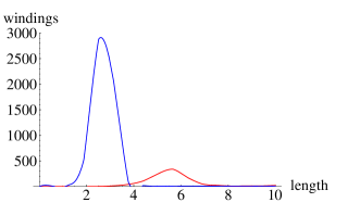
Figure 7: Number and length scale of windings a few time units after winding formation in units of $m_{\phi}^{-1}$. Both use $F_{0}=0.5$, but have different radion mass: $m_{F}=4.0\,m_{\phi}$ on the left and $m_{F}=2.0\,m_{\phi}$ on the right. The length scale relevant for baryogenesis, $l_{sph}$, is in the range of $6\,m_{\phi}^{-1}$. The total length for the simulation was $10^{5}\,m_{\phi}^{-1}$.

It would be interesting to use numerical methods on the classical 3+1 dimensional $SU(2)$ theory to track the Chern-Simons and Higgs winding numbers. The dependence of these quantities on the radion mass should unambiguously confirm or refute the model. In addition, this calculation would provide a more concrete estimate of the range of baryon to entropy ratios possible.

VI Conclusion

We have shown that baryogenesis can occur in the two-brane Randall-Sundrum model with radion preheating providing the departure from equilibrium. Another source of CP violation is needed, and as mentioned, investigations of bulk CP violation may prove interesting. One of the successes of this model is that preheating occurs naturally at the energy scale for sphaleron transitions to generate the asymmetry, but not wash it out.

Furthermore, the existence of a baryon asymmetry in our universe implies an upper bound on the radion mass. For a sufficiently large radion mass, the preheating band does not extend down to sphaleron length scales, unless the radion energy exceeds the thermal washout limit. We conclude that the radion mass should not be much larger than three times the Higgs mass, if the baryon asymmetry is to arise from this model.

*

Appendix A Number Density Operator

We calculate here the expectation value of the number density operator, $\langle 0|\hat{a}^{\dagger}_{k}(t)\hat{a}_{k}(t)|0\rangle$, for a massive scalar field coupled to the radion, i.e. for action (11). First, let us change the notation slightly to ease this calculation. We decompose the scalar:

$$\phi(t,\vec{x})=\int\frac{d^{3}k}{(2\pi)^{3/2}}\hat{\phi}_{k}(t)e^{-i\vec{k}\cdot\vec{x}},$$ (32)

where

$$\hat{\phi}_{k}(t)=U_{k}(t)\hat{a}_{k}+U^{*}_{-k}(t)\hat{a}^{\dagger}_{-k}.$$ (33)

We decompose the conjugate momentum, $\pi(t,\vec{x})$, in the analogous manner and find

$$\hat{\pi}_{k}(t)=e^{-F(t)/\Lambda}\left(\dot{U}_{k}(t)\hat{a}_{k}+\dot{U}^{*}_{-k}(t)\hat{a}^{\dagger}_{-k}\right).$$ (34)

We have assumed that the radion is independent of the spatial coordinate in anticipation of homogeneous oscillations.

This decomposition is in terms of operators which annihilate the initial vacuum, $\hat{a}_{k}|0\rangle=0$. We seek an expression for time dependent operators, $\hat{a}_{k}(t)$, in terms of the initial time operators so that we may calculate the number of particles relative to the initial vacuum. The time dependent (Heisenberg picture) operators must satisfy the equation of motion

$$i\frac{d}{dt}\hat{a}_{k}(t)=\left[\hat{a}_{k}(t),H(t)\right],$$ (35)

where $H(t)$ is the Hamiltonian. The Hamiltonian can be written in terms of $\hat{\phi}_{k}(t)$ and $\hat{\pi}_{k}(t)$:

$$H(t)= \frac{1}{2}\int\frac{d^{3}k}{(2\pi)^{3/2}}\Big{[}e^{F(t)/\Lambda}\hat{\pi}_{k}(t)\hat{\pi}_{-k}(t)$$ (36)

$$\qquad+e^{-F(t)/\Lambda}\omega_{k}^{2}(t)\hat{\phi}_{k}(t)\hat{\phi}_{-k}(t)\Big{]}.$$

As in the main text, $\omega_{k}^{2}(t)=k^{2}+m_{\phi}^{2}e^{-F(t)/\Lambda}$. We may look for a solution by making the ansatz:

$$\hat{a}_{k}(t)=g(t)\hat{\pi}_{k}(t)+h(t)\hat{\phi}_{k}(t).$$ (37)

This guess is motivated by the form of a Bogolubov transformation and the knowledge that $\hat{\pi}_{k}(t)$ and $\hat{\phi}_{k}(t)$ contain all of the degrees of freedom of the system.

From the initial conditions, $\hat{a}_{k}(t\!=\!0)=\hat{a}_{k}$, and

$${dU_{k}\over dt}(0)=-i\omega_{k}(0)U_{k}(0),\quad U_{k}(0)=\frac{e^{F(0)/2/\Lambda}}{\sqrt{2\omega_{k}(0)}},$$ (38)

as in equation (15), we find the initial values:

$$g(0)=iU^{*}_{k}(0)\quad h(0)=-ie^{-F(0)/\Lambda}\dot{U}^{*}_{k}(0).$$ (39)

Finally, using the standard equal time commutation relations for the field, $[\hat{\phi}_{\vec{k}}(t),\hat{\pi}_{\vec{p}}(t)]=i(2\pi)^{3}\delta^{3}(\vec{k}+\vec{p})$ we may evaluate the equation of motion for $\hat{a}_{k}(t)$. The result is simple:

$${d\over dt}g(t)=0={d\over dt}h(t).$$ (40)

We now use the form for the oscillating radion given in the text in equation (12) and evaluate the number operator from the ansatz (37):

$$\langle N_{k}(t)\rangle=\langle 0|\hat{a}_{k}^{\dagger}(t)\hat{a}_{k}(t)|0\rangle=$$

$$\quad{e^{-F_{0}}\over 2\omega_{k}(0)}\left[e^{2F_{0}\left[1-\cos(m_{F}t)\right]}|\dot{U}_{k}(t)|^{2}+\omega_{k}^{2}(0)|U_{k}(t)|^{2}\right]\ \$$

$$\quad-{ie^{-F_{0}\cos(m_{F}t)}\over 2}\left[U_{k}^{*}(t)\dot{U}_{k}(t)-\dot{U}_{k}^{*}(t)U_{k}(t)\right].\$$ (41)

- (1) M. Trodden, “Electroweak baryogenesis,” Rev. Mod. Phys. 71, 1463 (1999) [arXiv:hep-ph/9803479]; A. G. Cohen, D. B. Kaplan and A. E. Nelson, “Progress in electroweak baryogenesis,” Ann. Rev. Nucl. Part. Sci. 43, 27 (1993) [arXiv:hep-ph/9302210]; V. A. Rubakov and M. E. Shaposhnikov, “Electroweak baryon number non-conservation in the early universe and in high-energy collisions,” Usp. Fiz. Nauk 166, 493 (1996) [Phys. Usp. 39, 461 (1996)] [arXiv:hep-ph/9603208].
- (2) L. Randall and R. Sundrum, “A large mass hierarchy from a small extra dimension,” Phys. Rev. Lett. 83, 3370 (1999) [hep-ph/9905221].
- (3) W. D. Goldberger and M. B. Wise, “Modulus stabilization with bulk fields,” Phys. Rev. Lett. 83, 4922 (1999) [arXiv:hep-ph/9907447].
- (4) H. Collins, R. Holman and M. R. Martin, “Radion induced brane preheating,” arXiv:hep-ph/0205240.
- (5) J. Traschen and R. Brandenberger, Phys. Rev. D 42, 2491 (1990); Y. Shtanov, J. Traschen and R. Brandenberger, Phys. Rev. D 51, 5438 (1995); L. Kofman, A. D. Linde and A. A. Starobinsky, “Reheating after inflation,” Phys. Rev. Lett. 73, 3195 (1994) [hep-th/9405187]; L. Kofman, A. D. Linde and A. A. Starobinsky, “Towards the theory of reheating after inflation,” Phys. Rev. D 56, 3258 (1997) [hep-ph/9704452]; D. Boyanovsky, H. J. de Vega and R. Holman, “Erice Lectures on Inflationary Reheating” in the Proceedings of the 5th. Erice Chalonge School on Astrofundamental Physics, N. Sánchez and A. Zichichi eds., World Scientific, 1997 [hep-ph/9701304].
- (6) N. Turok and J. Zadrozny, “Electroweak Baryogenesis In The Two Doublet Model,” Nucl. Phys. B 358, 471 (1991); N. Turok and J. Zadrozny, “Dynamical Generation Of Baryons At The Electroweak Transition,” Phys. Rev. Lett. 65, 2331 (1990).
- (7) A. Lue, K. Rajagopal and M. Trodden, “Semi-analytical approaches to local electroweak baryogenesis,” Phys. Rev. D 56, 1250 (1997) [arXiv:hep-ph/9612282].
- (8) C. Charmousis, R. Gregory and V. A. Rubakov, “Wave function of the radion in a brane world,” Phys. Rev. D 62, 067505 (2000) [arXiv:hep-th/9912160].
- (9) P. Creminelli, A. Nicolis and R. Rattazzi, “Holography and the electroweak phase transition,” JHEP 0203, 051 (2002) [arXiv:hep-th/0107141].
- (10) L. M. Krauss and M. Trodden, “Baryogenesis below the electroweak scale,” Phys. Rev. Lett. 83, 1502 (1999) [arXiv:hep-ph/9902420];
- (11) J. Garcia-Bellido, D. Y. Grigoriev, A. Kusenko and M. E. Shaposhnikov, “Non-equilibrium electroweak baryogenesis from preheating after inflation,” Phys. Rev. D 60, 123504 (1999) [arXiv:hep-ph/9902449].
- (12) D. Boyanovsky, D. Cormier, H. J. de Vega, R. Holman, A. Singh and M. Srednicki, “Scalar field dynamics in Friedman Robertson Walker spacetimes,” Phys. Rev. D 56, 1939 (1997) [arXiv:hep-ph/9703327].
- (13) M. Carena and H. E. Haber, “Higgs Boson Theory and Phenomenology,” arXiv:hep-ph/0208209.
- (14) A. Rajantie, P. M. Saffin and E. J. Copeland, “Electroweak preheating on a lattice,” Phys. Rev. D 63, 123512 (2001) [arXiv:hep-ph/0012097].
- (15) J. Garcia-Bellido and D. Y. Grigoriev, “Inflaton-induced sphaleron transitions,” JHEP 0001, 017 (2000) [arXiv:hep-ph/9912515]; J. M. Cornwall and A. Kusenko, “Baryon number non-conservation and phase transitions at preheating,” Phys. Rev. D 61, 103510 (2000) [arXiv:hep-ph/0001058].
- (16) G. D. Moore, “Problems with lattice methods for electroweak preheating,” JHEP 0111, 021 (2001) [arXiv:hep-ph/0109206].
- (17) M. E. Peskin and D. V. Schroeder, “An Introduction To Quantum Field Theory,” Reading, USA: Addison-Wesley (1995) 842 p.
- (18) J. Smit and A. Tranberg, “Chern-Simons number asymmetry from CP violation at electroweak tachyonic preheating,” arXiv:hep-ph/0211243.
- (19) J. M. Cline and H. Firouzjahi, “Brane-world cosmology of modulus stabilization with a bulk scalar field,” Phys. Rev. D 64, 023505 (2001) [arXiv:hep-ph/0005235].