Mass predictions based on a supersymmetric SU(5) fixed point

Abstract

I examine the possibility that the third generation fermion masses are determined by an exact fixed point of the minimal supersymmetric SU(5) model. When one-loop supersymmetric thresholds are included, this unified fixed point successfully predicts the top quark mass, $175\pm 2$ GeV, as well as the weak mixing angle. The bottom quark mass prediction is sensitive to the supersymmetric thresholds; it approaches the measured value for $\mu<0$ and very large unified gaugino mass. The experimental measurement of the tau lepton mass determines $\tan\beta$, and the strong gauge coupling and fine structure constant fix the unification scale and the unified gauge coupling.

I Introduction

The measurement of the top quark mass at Fermilab in 1995 Groom:in completed a search that started nearly a hundred years ago with the measurement of the electron mass. Although neutrino masses still remain to be accurately measured, we already have the most important pieces of the puzzle of fermion masses. A satisfactory theory to explain the standard model (SM) fermion masses, however, is still lacking. The disparity in the mass scales of the third generation fermions and the first and second generation fermions, as well as their mixing angles, suggest that different mechanisms may be responsible for the masses of third generation, and first and second generation fermions. Indeed, an explanation of third generation fermion masses may be necessary to understand first and second generation fermion masses.

It is widely hoped that fermion masses and mixing angles will be explained, or at least reduced, by some grand unified theory (GUT)Georgi:sy . In this case, to obtain predictions for the values of masses, gauge couplings and mixing angles, the predictions for the boundary conditions of the unified theory at the GUT scale would be extended, using the renormalization group equations, from the unification scale down to the electroweak scale. The current grand unified theories, however, reduce the number of parameters but they do not make definite predictions for the Yukawa couplings at the unification scale. These couplings must be fit to the experimental measurements. This approach has been extensively used in the literature to study third generation fermion masses in the context of supersymmetric grand unified models (SUSY GUTs) susyguts . It has been found that the unification scale Yukawa couplings can be adjusted to fit the measured top, bottom and tau fermion masses SO10 ; texturas .

There is an alternative idea, not incompatible with the previous approach, which can make unified theories more predictive. If the renormalization group equations describing the evolution of the various couplings in the theory possess an infrared fixed point, then some of these couplings could be swept towards this fixed point Pendleton:as ; masso . M. Lanzagorta and G.G. Ross Lanzagorta:1995gp have pointed out that the fixed point structure of the unified theory beyond the standard model may play a very important role in the determination of the Yukawa couplings at the gauge unification scale. It was argued that the evolution towards the fixed point may occur more rapidly in some unified theories than in the low-energy theory due to their larger field content and the possible lack of asymptotic freedom. Therefore, even though the “distance” between the grand unification scale and the Planck scale (or the compactification scale) is much less than the distance between the electroweak scale and the grand unification scale, the unified fixed point could play a significant role in determining the couplings at the unification scale, regardless of their values in the underlying “Theory of Everything.” This possibility would make the unified theory much more predictive because the Yukawa couplings at the unification scale may be determined in terms of the unified gauge coupling according to the unified gauge group and the multiplet content of the model.

The purpose of this paper is to study the possibility that the third generation fermion masses are determined by the fixed point structure of the minimal supersymmetric SU(5) model. We will not analyze here whether or not nature can reach a fixed point at the unification scale, because ultimately that analysis depends on assumptions about the still unknown physics at yet higher energy scales, perhaps at the Planck scale. Instead, we will adopt a phenomenological approach: we will assume that at the unification scale the SU(5) model is at a fixed point, and we will study the low-energy implications of our assumption.

We will not address here the problems that afflict the minimal supersymmetric SU(5) model: namely, the doublet-triplet splitting problem, the strong experimental constraints on proton decay, the generation of neutrino masses, and the lack of predictivity in the flavor sector. Solutions have been proposed for each of these problems, and entail complicating the minimal SU(5) model Masina:2001pp . Since our aim is to explore a new idea, in this paper we will use the smallest simple group in which one can embed the standard model gauge group: the minimal third-generation supersymmetric SU(5) model. We think that the idea can be extended to non minimal grand unified models, where the problems that afflict minimal SU(5) may find a resolution.

This paper is organized as follows. We begin in Sec. II with the calculation of the fixed points for the Yukawa sector of the model. We find only one phenomenologically interesting fixed point and analyze its mass predictions, first by neglecting low-energy supersymmetric thresholds. In Sec. III we calculate the associated fixed point in the soft SUSY breaking sector of the model. In Sec. IV we study the fixed point implications for the breaking of the SU(5) symmetry. In Sec. V we study the characteristic low-energy supersymmetric spectra predicted by the fixed point. In Sec. VI we study the fermion mass predictions including the low-energy supersymmetric thresholds. Here, we also analyze the dependence of the predictions on the unified gaugino mass and on the sign of the $\mu$-term. In Sec. VII we briefly analyze the fixed point predictions for fermion masses in the context of non minimal SU(5) models with additional particle content. We conclude in Sec. IX with a brief summary of our results.

II Fixed points for the minimal supersymmetric SU(5)

We begin our calculation of one-loop fixed points with a brief review of the model to set up our conventions and notation. The superpotential of the minimal one-generation supersymmetric SU(5) model, omitting SU(5) indices, is given by Witten:nf ; Sakai:1981gr ; Dimopoulos:1981zb

$${\cal W}_{\rm SU(5)} = \mu_{\Sigma}~{}tr\Sigma^{2}+\frac{1}{6}\lambda_{\Sigma}~{}tr\Sigma^{3}+\mu_{H}~{}{\cal H}_{5}{\cal H}_{\overline{5}}$$ (1)

$$+ \lambda_{H}{\cal H}_{\overline{5}}\Sigma{\cal H}_{5}+\frac{1}{4}\lambda_{t}\psi_{10}\psi_{10}{\cal H}_{5}+\sqrt{2}\lambda_{b}\psi_{10}\psi_{\overline{5}}{\cal H}_{\overline{5}},$$

where $\psi_{10}$ and $\psi_{\overline{5}}$ are matter chiral superfields belonging to representations 10 and $\overline{{\bf 5}}$ of SU(5), respectively. As in the supersymmetric generalization of the standard model, to generate fermion masses we need two sets of Higgs superfields, ${\cal H}_{5}$ and ${\cal H}_{\overline{5}}$, belonging to representations 5 and $\overline{{\bf 5}}$ of SU(5). The Higgs superfield in the adjoint 24-dimensional representation, $\Sigma$, is chosen to allow the existence of a realistic breaking of the SU(5) symmetry down to the SM group, ${\rm G}_{\rm SM}\equiv SU(3)_{C}\times SU(2)_{L}\times U(1)_{Y}$. Typically, fixed points appear for ratios of couplings, such as ratios of Yukawa couplings to gauge couplings, and are known generically as Pendleton-Ross fixed points. The renormalization group equations (RGEs) for the SU(5) Yukawa couplings, valid above the GUT scale, are given by pomarol ; strumia ; Bagger:1999ty

$$\frac{d}{dt}\left(\begin{array}[]{c}{\lambda}_{t}^{2}\\ {\lambda}_{b}^{2}\\ {\lambda}^{2}_{H}\\ {\lambda}^{2}_{\Sigma}\end{array}\right)=\left(\begin{array}[]{c}{\lambda}_{t}^{2}\\ {\lambda}_{b}^{2}\\ {\lambda}^{2}_{H}\\ {\lambda}^{2}_{\Sigma}\end{array}\right)^{T}\left(\left(\begin{array}[]{cccc}9&4&24/5&0\\ 3&10&24/5&0\\ 3&4&53/5&21/20\\ 0&0&3&63/20\end{array}\right)\left(\begin{array}[]{c}{\lambda}_{t}^{2}\\ {\lambda}_{b}^{2}\\ {\lambda}^{2}_{H}\\ {\lambda}^{2}_{\Sigma}\end{array}\right)-\left(\begin{array}[]{c}96/5\\ 84/5\\ 98/5\\ 30\end{array}\right)g^{2}\right),$$ (2)

where $T$ denotes the matrix transpose, $t=1/8\pi^{2}\log\Lambda$, and $\Lambda$ is the renormalization scale. The RGE for the SU(5) unified gauge coupling is given by

$$\frac{dg^{2}}{dt}=bg^{4},$$ (3)

with $b=-3$ in the minimal model. The RGEs for the ratios of Yukawa couplings to the unified gauge coupling can be easily calculated from Eqs. (2) and 3:

$$\frac{1}{g^{2}}\frac{d}{dt}\left(\begin{array}[]{c}\widetilde{\lambda}_{t}^{2}\\ \widetilde{\lambda}_{b}^{2}\\ \widetilde{\lambda}^{2}_{H}\\ \widetilde{\lambda}^{2}_{\Sigma}\end{array}\right)=\left(\begin{array}[]{c}\widetilde{\lambda}_{t}^{2}\\ \widetilde{\lambda}_{b}^{2}\\ \widetilde{\lambda}^{2}_{H}\\ \widetilde{\lambda}^{2}_{\Sigma}\end{array}\right)^{T}\left(\left(\begin{array}[]{cccc}9&4&24/5&0\\ 3&10&24/5&0\\ 3&4&53/5&21/20\\ 0&0&3&63/20\end{array}\right)\left(\begin{array}[]{c}\widetilde{\lambda}_{t}^{2}\\ \widetilde{\lambda}_{b}^{2}\\ \widetilde{\lambda}^{2}_{H}\\ \widetilde{\lambda}^{2}_{\Sigma}\end{array}\right)-\left(\begin{array}[]{c}96/5+b\\ 84/5+b\\ 98/5+b\\ 30+b\end{array}\right)\right),$$ (4)

where we have defined

$$\widetilde{\lambda}_{t}^{2}=\frac{\lambda_{t}^{2}}{g^{2}},\qquad\widetilde{\lambda}_{b}^{2}=\frac{\lambda_{b}^{2}}{g^{2}},\qquad\widetilde{\lambda}^{2}_{H}=\frac{\lambda^{2}_{H}}{g^{2}},\qquad\widetilde{\lambda}^{2}=\frac{\lambda^{2}_{\Sigma}}{g^{2}}.$$ (5)

fixed point	$\widetilde{\lambda}_{t}^{2}$	$\widetilde{\lambda}^{2}_{b}$	$\widetilde{\lambda}^{2}_{H}$	$\widetilde{\lambda}^{2}_{\Sigma}$
1	$0~{}(R)$	$0~{}(R)$	$0~{}(R)$	$0~{}(R)$
2	$0~{}(R)$	$0~{}(R)$	$0~{}(R)$	$60/7~{}(A)$
3	$0~{}(R)$	$0~{}(R)$	$83/53~{}(A)$	$0~{}(R)$
4	$0~{}(R)$	$69/50~{}(A)$	$0~{}(R)$	$0~{}(R)$
5	$9/5~{}(A)$	$0~{}(R)$	$0~{}(R)$	$0~{}(R)$
6	$0~{}(R)$	$0~{}(R)$	$19/24~{}(A)$	$985/126~{}(A)$
7	$0~{}(R)$	$69/50~{}(A)$	$0~{}(R)$	$60/7~{}(A)$
8	$9/5~{}(A)$	$0~{}(R)$	$0~{}(R)$	$60/7~{}(A)$
9	$767/675~{}(A)$	$0~{}(R)$	$56/45~{}(A)$	$0~{}(R)$
10	$0~{}(R)$	$333/434~{}(A)$	$277/217~{}(A)$	$0~{}(R)$
11	$0~{}(R)$	$5/4~{}(A)$	$13/48~{}(A)$	$2095/252~{}(A)$
12	$124/75~{}(A)$	$0~{}(R)$	$11/40~{}(A)$	$349/42~{}(A)$
13	$89/65~{}(A)$	$63/65~{}(A)$	$0~{}(R)$	$0~{}(R)$
14	$89/65~{}(A)$	$63/65~{}(A)$	$0~{}(A)$	$60/7~{}(A)$
15	$132/95~{}(A)$	$94/95~{}(A)$	$-25/456~{}(R)$	$20645/2394~{}(A)$
16	$2533/2605~{}(A)$	$1491/2605~{}(A)$	$560/521~{}(A)$	$0~{}(R)$

Table 1: One-loop fixed points and their stability properties for the minimal supersymmetric SU(5) model.

We present in Table 1 the list of fixed points, along with their respective solutions and stability character in the infrared Allanach:1997bh , (A) if the direction is attractive, and (R) if it is repulsive. We observe that 12 out of the 16 solutions have vanishing $\lambda_{t}$ or $\lambda_{b}$ and are phenomenologically not viable, as they predict a zero mass for the top quark, or for the bottom quark and tau lepton. Moreover, it is known that the dimension-five operators induced by the colored Higgs triplet give large contributions to the proton decay rate proton . To suppress such operators, the mass of the colored Higgs triplet has to be heavy, implying $\lambda_{H}>g$. This then excludes solutions 13 and 14, which have $\lambda_{H}=0$. Solution 15 is a non physical solution with $\lambda_{H}^{2}<0$. Only one interesting solution remains, solution 16, which predicts

$$\frac{\lambda_{t}^{2}}{g^{2}}=\frac{2533}{2605},\qquad\frac{\lambda_{b}^{2}}{g^{2}}=\frac{1491}{2605},\qquad\frac{\lambda^{2}_{H}}{g^{2}}=\frac{560}{521},\qquad\frac{\lambda^{2}_{\Sigma}}{g^{2}}=0.$$ (6)

We observe that this fixed point predicts $\lambda_{H}=1.03675~{}g$, overcoming the previous naïve constraint on proton decay. Moreover, it predicts interesting values for the top and bottom-tau Yukawa couplings at the unification scale, $\lambda_{t}=0.98608~{}g$ and $\lambda_{b}=0.75654~{}g$ (later we will study, in detail, the fermion masses derived from these predictions). On the other hand, the fixed point predicts $\lambda_{\Sigma}=0$, while in principle we need $\lambda_{\Sigma}\neq 0$ if we want to break the SU(5) symmetry. Furthermore, the directions $t$, $b$ and $H$ are attractive, while the direction $\Sigma$ is repulsive. One can wonder to what extent it is consistent to study predictions coming from this fixed point if the direction $\lambda_{\Sigma}=0$ is not attractive. If we assume that the $\left|\lambda_{\Sigma}\right|$ coupling is much less than $g$, the RGE can be approximately solved as

$$\frac{1}{g^{2}}\frac{d}{dt}\widetilde{\lambda}^{2}_{\Sigma}\simeq-27~{}\widetilde{\lambda}^{2}_{\Sigma}\longrightarrow\widetilde{\lambda}^{2}_{\Sigma}(\Lambda_{G})\simeq\widetilde{\lambda}^{2}_{\Sigma}(\Lambda_{P})\times\left(\frac{\Lambda_{P}}{\Lambda_{G}}\right)^{27/8\pi^{2}}\simeq 10~{}\widetilde{\lambda}^{2}_{\Sigma}(\Lambda_{P}).$$ (7)

Then, $\lambda_{\Sigma}$ is only a slowly decreasing function of the scale. For instance, assuming that $\widetilde{\lambda}_{\Sigma}^{2}(\Lambda_{P})<10^{-3}$ at the Planck scale, we obtain $\widetilde{\lambda}_{\Sigma}^{2}(\Lambda_{G})<10^{-2}$ at the GUT scale. We observe that the coupling $\lambda_{\Sigma}$ is not directly coupled to $\lambda_{t}$ and $\lambda_{b}$ and is only weakly coupled to $\lambda_{H}$; so it is interesting to analyze the perturbation on the exact fixed point predictions coming from a small deviation along the direction $\lambda_{\Sigma}=0$. The fixed point for the truncated system $(\lambda_{t},\lambda_{b},\lambda_{H})$, assuming that $\lambda_{\Sigma}$ is a constant parameter, can be calculated from Eq. (4), and we obtain

$$\frac{\lambda_{t}^{2}}{g^{2}}=\frac{2533}{2605}+\frac{126}{2605}\frac{\lambda_{\Sigma}^{2}}{g^{2}},\qquad\frac{\lambda_{b}^{2}}{g^{2}}=\frac{1491}{2605}+\frac{126}{2605}\frac{\lambda_{\Sigma}^{2}}{g^{2}},\qquad\frac{\lambda^{2}_{H}}{g^{2}}=\frac{560}{521}-\frac{273}{2084}\frac{\lambda_{\Sigma}^{2}}{g^{2}}.$$ (8)

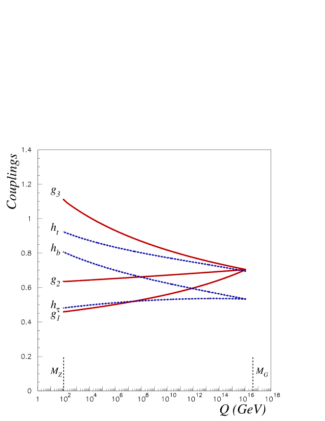
Figure 1: Two-loop gauge and Yukawa coupling evolution from the unification scale to $M_{Z}$ scale for the exact $SU(5)$ fixed point boundary conditions. The plot corresponds to point 1 in Table 6.

From these equations we see that the naïve phenomenological constraint on proton decay, $\lambda_{H}>g$, implies an upper bound on $\lambda_{\Sigma}^{2}$ given by $\lambda_{\Sigma}^{2}<4/7~{}g^{2}=0.5714~{}g^{2}$. Therefore, for the fixed point to become phenomenologically viable, the coupling $\lambda_{\Sigma}$ must be much smaller than $g$; otherwise we cannot overcome the constraints on proton decay. If $\lambda_{\Sigma}^{2}$ is less than $0.5~{}g^{2}$, the fixed point predictions for $\lambda_{t}$ and $\lambda_{b}$ at the GUT scale, given in Eqs. (8), are constrained to be less than $2\%$ away from the exact fixed point predictions. This perturbation, when extrapolated to the electroweak scale, affects slightly the predictions for fermion masses, which turn out to be less than $1\%$ away from the exact fixed point predictions. Therefore, small perturbations in the $\lambda_{\Sigma}$ direction do not affect seriously the exact fixed point predictions, since the fermion Yukawa couplings are not directly coupled to $\lambda_{\Sigma}$. From now on we will assume that at the GUT scale $\lambda_{\Sigma}$ is much smaller than the other couplings:

$$\left|\lambda_{\Sigma}\right|<<\lambda_{t},\lambda_{b},\lambda_{H},g.$$ (9)

In this case it makes sense to study the predictions ensuing from the exact fixed point given by Eq. (6), even when $\lambda_{\Sigma}=0$ is a non attractive direction.

II.1 Numerical results without supersymmetric thresholds

We now turn to an analysis of the fixed point predictions for the third generation fermion masses and the standard model gauge couplings. We will assume that the SU(5) symmetry breaks to the standard model group, $G_{SM}$, at the GUT scale and, temporarily, ignore the effects of the low-energy supersymmetric thresholds to gauge and Yukawa coupling predictions. We assume that $\lambda_{\Sigma}<<g$, so that our model has only three basic parameters: the unification scale $M_{G}$, the unified gauge coupling $g$, and the ratio of vacuum expectation values in the MSSM, $\tan\beta$. $M_{G}$ and $g$ are high energy model parameters while $\tan\beta$ is a low-energy parameter. Below $M_{G}$, the effective theory is the third generation MSSM given by the superpotential

$${\cal W}_{\rm MSSM}=\mu~{}{\cal H}_{u}{\cal H}_{d}+h_{t}{\cal Q}{\cal H}_{u}{\cal U}+h_{b}{\cal Q}{\cal H}_{d}{\cal D}+h_{\tau}{\cal L}{\cal H}_{d}{\cal E},$$ (10)

where the Yukawa couplings at the GUT scale are determined by the boundary conditions given by the SU(5) fixed point, Eq. (6). We will scan the parameter space and will require that the strong gauge coupling, the fine structure constant and the tau mass be in the measured range Groom:in :

$$\widehat{\alpha}_{e}(m_{Z})^{-1} = 127.934\pm 0.027,$$ (11)

$$\alpha_{s}(m_{Z}) = 0.1172\pm 0.0020,$$ (12)

$$m_{\tau} = 1.77703~{}{\rm GeV}.$$ (13)

model parameters
$M_{G}\times 10^{-16}$ (GeV)	$1.81\pm 0.20$
$g_{G}$	$0.725\pm 0.001$
$\tan\beta$	$47.98\pm 0.03$
experimental constraints
$\widehat{\alpha}_{e}(m_{Z})^{-1}_{\overline{\rm MS}}$	$127.934\pm 0.027$
$\alpha_{s}(m_{Z})_{\overline{\rm MS}}$	$0.1172\pm 0.0020$
$m_{\tau}$ (GeV)	$1.77703$
theoretical predictions
$\widehat{s}_{W}^{2}(m_{Z})_{\overline{\rm MS}}$	$0.2334\pm 0.0005$
$m_{t}$ (GeV)	$181.5\pm 1.2$
$m_{b}(m_{Z})_{\overline{\rm MS}}$ (GeV)	$3.20\pm 0.02$

Table 2: Exact SU(5) fixed point predictions without including superspectrum thresholds. We fit the central values of $\widehat{\alpha}_{e}(m_{Z})^{-1}_{\overline{\rm MS}}$, $\alpha_{s}(m_{Z})_{\overline{\rm MS}}$ and $m_{\tau}$ with experimental uncertainties and obtain three theoretical predictions for $\widehat{s}_{W}^{2}(m_{Z})$, $m_{t}$ and $m_{b}(m_{Z})$, which must be compared with the experimental measurements $m_{t}=174.3\pm 5.1$ GeV, $m_{b}(m_{Z}^{>})_{\overline{\rm MS}}=2.86\pm 0.2$ GeV and $\widehat{s}_{W}^{2}(m_{Z})_{\overline{\rm MS}}=0.23117(16)$.

model parameters
$M_{G}\times 10^{-16}$ (GeV)	1.8139
$g$	0.7255
$\tan\beta$	47.9864
MSSM Yukawa couplings at $M_{G}$ (fixed point values)
$h_{t}(M_{G})$	0.71548
$h_{b}(M_{G})$	0.54893
$h_{\tau}(M_{G})$	0.54893
MSSM dimensionless couplings at $M_{Z}$
$g_{1}(M_{Z})$	0.46213
$g_{2}(M_{Z})$	0.64873
$g_{3}(M_{Z})$	1.21943
$h_{t}(M_{Z})$	0.98845
$h_{b}(M_{Z})$	0.87367
$h_{\tau}(M_{Z})$	0.48392
experimental constraints
$\alpha_{e}(m_{Z})^{-1}_{\overline{\rm MS}}$	127.925
$\alpha_{s}(m_{Z})_{\overline{\rm MS}}$	0.11721
$m_{\tau}$ (GeV)	1.77703
theoretical predictions
$s_{W}^{2}(m_{Z})_{\overline{\rm MS}}$	0.23340
$m_{t}$ (GeV)	181.631
$m_{b}(m_{Z})_{\overline{\rm MS}}$ (GeV)	3.202

Table 3: Representative point of the fit for the exact SU(5) fixed point without supersymmetric thresholds.

Roughly speaking, the strong gauge coupling and the fine structure constant determine the values of the unification scale and the unified gauge coupling. Once we know $M_{G}$ and $g$, the fixed point predicts the value of the tau Yukawa coupling at the $m_{Z}$ scale. We can then determine $\tan\beta$ using the tau mass measurement and the tree level tau mass formula in the MSSM,

$$m_{\tau}(m_{Z}^{>})=h_{\tau}(m_{Z})v(m_{Z})\cos\beta.$$ (14)

Here, $v(m_{Z})=2m_{W}/g_{2}(m_{Z})$, $g_{2}(m_{Z})$ is the weak coupling constant at $m_{Z}$, and $m_{\tau}(m_{Z}^{>})$ is the tau running mass at $m_{Z}$ above the electroweak threshold. The tau pole mass, $m_{\tau}$, must be related to the running mass below the electroweak threshold , $m_{\tau}(m_{Z}^{<})$, including QED corrections Arason:1991ic

$$m_{\tau}(m_{Z}^{<})=m_{\tau}\left\{1-\frac{\alpha_{e}(m_{Z})}{\pi}\left(1+\frac{3}{4}\ln\left(\frac{m_{Z}^{2}}{m_{\tau}(m_{Z}^{<})}\right)\right]\right\}.$$ (15)

We must include the effects of $W$ and $Z$ bosons to obtain the running mass just above the electroweak threshold,

$$m_{\tau}(m_{Z}^{>})=m_{\tau}(m_{Z}^{<})\left(1+\Delta^{\tau}_{SM}\right),$$ (16)

where the expression for the electroweak thresholds, $\Delta^{\tau}_{SM}$, is given in Ref. Wright:1994qb and is very small, approximately $0.1\%$. Using the particle data group (PDG) central values we find that the tau running mass is $m_{\tau}(m_{Z}^{<})=1.7463$ GeV just below $m_{Z}$ and $m_{\tau}(m_{Z}^{>})=1.7482$ GeV just above $m_{Z}$. Once we know $\tan\beta$, we obtain, along with the weak mixing angle, two additional predictions from the SU(5) fixed point: the top and bottom quark masses. The running bottom quark mass just above $m_{Z}$ in the dimensional reduction scheme ($\overline{\rm DR}$) is computed using the tree level MSSM formula for the bottom mass,

$$m_{b}^{\overline{\rm DR}}(m_{Z}^{>})=h_{b}(m_{Z})v(m_{Z})\cos\beta.$$ (17)

To convert $m_{b}^{\overline{\rm DR}}(m_{Z}^{>})$ to the minimal substraction scheme ($\overline{\rm MS}$) we use the expression Baer:2002ek

$$m_{b}^{\overline{\rm DR}}(m_{Z}^{>})=m_{b}^{\overline{\rm MS}}(m_{Z}^{>})\left[1-\frac{1}{3}\frac{\alpha_{s}^{\overline{\rm MS}}(m_{Z})}{\pi}-\frac{29}{72}\left(\frac{\alpha_{s}^{\overline{\rm MS}}(m_{Z})}{\pi}\right)^{2}\right].$$ (18)

We note that to compute $\alpha_{s}^{\overline{\rm MS}}(m_{Z})$ we convert $\alpha_{s}^{\overline{\rm DR}}(m_{Z})$ using Antoniadis:1982vr

$$\frac{1}{\alpha_{s}^{\overline{\rm DR}}(m_{Z})}=\frac{1}{\alpha_{s}^{\overline{\rm MS}}(m_{Z})}-\frac{1}{4\pi}.$$ (19)

To obtain the experimental bottom running mass just above $m_{Z}$, $m_{b}^{\overline{\rm MS}}(m_{Z}^{>})$, we start with the experimental value for $m_{b}^{\overline{\rm MS}}(m_{b}^{\overline{\rm MS}})$; using the analytical solution of the SM RGE for the running mass we compute the bottom running mass just below the electroweak threshold. Then we include the electroweak loops, $\Delta^{b}_{SM}$, to obtain the running mass just above $m_{Z}$,

$$m_{b}^{\overline{\rm MS}}(m_{Z}^{>})=m_{b}^{\overline{\rm MS}}(m_{Z}^{<})\left(1+\Delta^{b}_{SM}\right).$$ (20)

Once again, the expression for the electroweak thresholds, $\Delta^{b}_{SM}$ is given in Wright:1994qb and is approximately $-0.4\%$. Using $m_{b}^{\overline{\rm MS}}(m_{b}^{\overline{\rm MS}})=4.2$ GeV and central PDG values for gauge couplings, we obtain $m_{b}^{\overline{\rm MS}}(m_{Z}^{<})=2.87$ GeV just below $m_{Z}$, and $m_{b}^{\overline{\rm MS}}(m_{Z}^{>})=2.86$ GeV just above $m_{Z}$, and after $\overline{\rm MS}$ to $\overline{\rm DR}$ conversion $m_{b}^{\overline{\rm DR}}(m_{Z}^{>})=2.82$ GeV. This is the value to which we should compare our prediction. The physical top quark mass is predicted using the formula

$$m_{t}=h_{t}(m_{t})v(m_{t})\sin\beta\left(1+\Delta_{\rm QCD}^{\rm t}\right),$$ (21)

where $\Delta_{\rm QCD}^{\rm t}$ stands for the gluon correction to the top mass evaluated at the $m_{t}$ scale. In the $\overline{\rm DR}$ scheme this is given by

$$\Delta_{\rm QCD}^{\rm t}=\frac{5}{3}\frac{\alpha_{s}(m_{t})}{\pi}+8.15\left(\frac{\alpha_{s}(m_{t})}{\pi}\right)^{2}+71.5\left(\frac{\alpha_{s}(m_{t})}{\pi}\right)^{3}.$$ (22)

We observe that the order $\alpha_{s}$ coefficient is $5/3$ in the $\overline{\rm DR}$ scheme and $4/3$ in the $\overline{\rm MS}$ scheme Tarrach:1980up . The order $\alpha_{s}^{2}$ coefficient in the $\overline{\rm DR}$ scheme has been computed from Ref. Avdeev:1997sz . The order $\alpha_{s}^{3}$ term is the coefficient computed in the $\overline{\rm MS}$ scheme and can be extracted from Ref. Melnikov:2000qh . The difference between $v(m_{t})$ and $v(M_{Z})$ is only of the order

$$v(m_{Z})-v(m_{t})\simeq\frac{2}{3}\ln\left(\frac{m_{t}}{m_{Z}}\right)~{}\hbox{\rm GeV},$$

which represents around $0.25$%. In practice, we implement this procedure numerically using two-loop MSSM RGEs for gauge and Yukawa couplings from the unification to the $m_{Z}$ scale rges ; isasugra . Our numerical results can be read off Table 2. The uncertainties in the model parameters and theoretical predictions shown in Table 2 are theoretical errors induced by uncertainties in the experimental constraints. Our fixed point predictions, neglecting supersymmetric thresholds, thus become

$$m_{t} = 181.6\pm 1.3~{}{\rm GeV},$$ (23)

$$m_{b}(m_{Z})_{\overline{\rm MS}} = 3.20\pm 0.03~{}{\rm GeV},$$ (24)

$$\widehat{s}_{W}^{2}(m_{Z})_{\overline{\rm MS}} = 0.2334\pm 0.0005.$$ (25)

These must be compared with the experimental measurements Groom:in

$$m_{t} = 174.3\pm 5.1~{}{\rm GeV},$$ (26)

$$m_{b}(m_{Z}^{>})_{\overline{\rm MS}} = 2.86\pm 0.2~{}{\rm GeV},$$ (27)

$$\widehat{s}_{W}^{2}(m_{Z})_{\overline{\rm MS}} = 0.23117(16).$$ (28)

Surprisingly, the tree level (i.e. with no SUSY thresholds) fixed point prediction is 3 % away from the experimental central value for the top mass and 4 % away from the experimental central value for the bottom mass. For comparision, we show in Table 3 the high-energy and low-energy coupling predictions for one of the central points of the fit. The relatively accurate prediction for the bottom mass at this stage is not a surprise, since the bottom–tau mass ratio is a successful classical prediction of SUSY GUTs when SUSY threshold corrections are not included bottomtau . Not taking into account these corrections, however, renders the classical prediction for the bottom-tau mass ratio irrelevant, since the contribution of SUSY thresholds to the bottom mass can be very important thresholds – as much as $\pm 40\%$ for large $\tan\beta$, depending on the sign of the $\mu$ term. The case of the top mass prediction is similar, although we had no reason, a priori, to expect a good agreement with data. This good prediction must also be considered only a provisional success, as we have ignored the effect of supersymmetric thresholds. For the moment, we do not know if the inclusion of these thresholds would spoil our interesting predictions. A predictive theory for the supersymmetry breaking sector is necessary in order to include these supersymmetric thresholds.

III minimal SU(5) fixed point and soft breaking

A realistic globally supersymmetric SU(5) model can be constructed Dimopoulos:1981zb , in which supersymmetry is broken explicitly, but softly, by terms of dimension less than four in the Lagrangian Girardello:1981wz . The scalar potential will contain the following SU(5)-invariant terms:

$${\cal V_{\rm SU(5)}} = m^{2}_{H_{\overline{5}}}\left|{h}_{\overline{5}}\right|^{2}+m^{2}_{H_{5}}\left|{h}_{5}\right|^{2}+m^{2}_{\Sigma}~{}{\rm tr}\left\{\sigma^{\dagger}\sigma\right\}+m^{2}_{5}\left|\phi_{\overline{5}}\right|^{2}+m^{2}_{10}~{}{\rm tr}\left\{\phi^{\dagger}_{10}\phi_{10}\right\}$$

$$+ \left[\frac{1}{6}A_{\Sigma}\lambda_{\Sigma}~{}{\rm tr}\sigma^{3}+A_{H}\lambda_{H}~{}h_{\overline{5}}\sigma h_{5}+\frac{1}{4}A_{t}\lambda_{t}\phi_{10}\phi_{10}{h}_{5}+\sqrt{2}A_{b}\lambda_{b}\phi_{10}\phi_{\overline{5}}{h}_{\overline{5}}\right.$$

$$+ \left.\frac{1}{2}M_{1/2}\lambda_{\alpha}\lambda_{\alpha}+B_{\Sigma}\mu_{\Sigma}~{}{\rm tr}\sigma^{2}+B_{H}\mu_{H}h_{5}h_{\overline{5}}+{\cal{\rm h.c.}}\right],$$

where $h_{5}$, $h_{\overline{5}}$, $\sigma$, $\phi_{\overline{5}}$ and $\phi_{10}$ are the scalar components of the superfields ${\cal H}_{u}$, ${\cal H}_{d}$, $\Sigma$, $\psi_{\overline{5}}$ and $\psi_{10}$, respectively, and $\lambda_{\alpha}$ are the SU(5) gaugino fields. It is known that the purpose of mass terms for matter and gaugino fields is to increase the mass of the still-unobserved MSSM spectra at low-energy. The soft sector parameters must be chosen with care to assure that the Hamiltonian is bounded from below and to obtain a desirable pattern of SU(5) breaking susysu5breaking . In principle the soft parameters are arbitrary. Interestingly, however, it has been pointed out that the existence of infrared stable fixed points for the Yukawa couplings implies (given asymptotic freedom) infrared stable fixed points for the soft parameters Jack:1998xw . Moreover, at this fixed point the dimensionful soft-breaking parameters are all determined by the gaugino mass. Special relationships then appear, and as a consequence a particular pattern of supersymmetric spectra emerges at low-energy if electroweak symmetry breaking can be achieved jackjones . We begin by analyzing the one-loop RGEs for the soft SUSY breaking parameters, with the goal of identifying their infrared fixed point associated with the fixed point of the Yukawa couplings. The fixed points for the trilinear soft parameters will appear for the ratios of trilinear parameters to the gaugino unified mass Lanzagorta:1995ai . The RGEs for these ratios are

$$\frac{1}{g^{2}}\frac{d}{dt}\left(\begin{array}[]{c}\widetilde{A}_{t}\\ \widetilde{A}_{b}\\ \widetilde{A}_{H}\\ \widetilde{A}_{\Sigma}\end{array}\right)=\left(\left(\begin{array}[]{cccc}9\widetilde{\lambda}_{t}^{2}-b&4\widetilde{\lambda}_{b}^{2}&24/5\widetilde{\lambda}^{2}_{H}&0\\ 3\widetilde{\lambda}_{t}^{2}&10\widetilde{\lambda}_{b}^{2}-b&24/5\widetilde{\lambda}^{2}_{H}&0\\ 3\widetilde{\lambda}_{t}^{2}&4\widetilde{\lambda}_{b}^{2}&53/5\widetilde{\lambda}^{2}_{H}-b&21/20\widetilde{\lambda}^{2}_{\Sigma}\\ 0&0&3\widetilde{\lambda}^{2}_{H}&63/20\widetilde{\lambda}^{2}_{\Sigma}-b\end{array}\right)\left(\begin{array}[]{c}\widetilde{A}_{t}\\ \widetilde{A}_{b}\\ \widetilde{A}_{H}\\ \widetilde{A}_{\Sigma}\end{array}\right)+\left(\begin{array}[]{c}96/5\\ 84/5\\ 98/5\\ 30\end{array}\right)\right),$$ (30)

where we have defined

$$\widetilde{A}_{t}=\frac{A_{t}}{M_{1/2}},\qquad\widetilde{A}_{b}=\frac{A_{b}}{M_{1/2}},\qquad\widetilde{A}_{H}=\frac{A_{H}}{M_{1/2}},\qquad\widetilde{A}_{\Sigma}=\frac{A_{\Sigma}}{M_{1/2}}.$$ (31)

We observe again, from Eq. (30), that the $\lambda_{\Sigma}$ is not coupled directly to $A_{t}$ and $A_{b}$ and is only weakly coupled to $A_{H}$. There will be a fixed point for the soft trilinears associated with the fixed point, Eq. (6), in the Yukawa sector given by

$$\frac{A_{t}}{M_{1/2}}=-1,\qquad\frac{A_{b}}{M_{1/2}}=-1,\qquad\frac{A_{H}}{M_{1/2}}=-1,\qquad\frac{A_{\Sigma}}{M_{1/2}}=-\frac{4650}{521}.$$ (32)

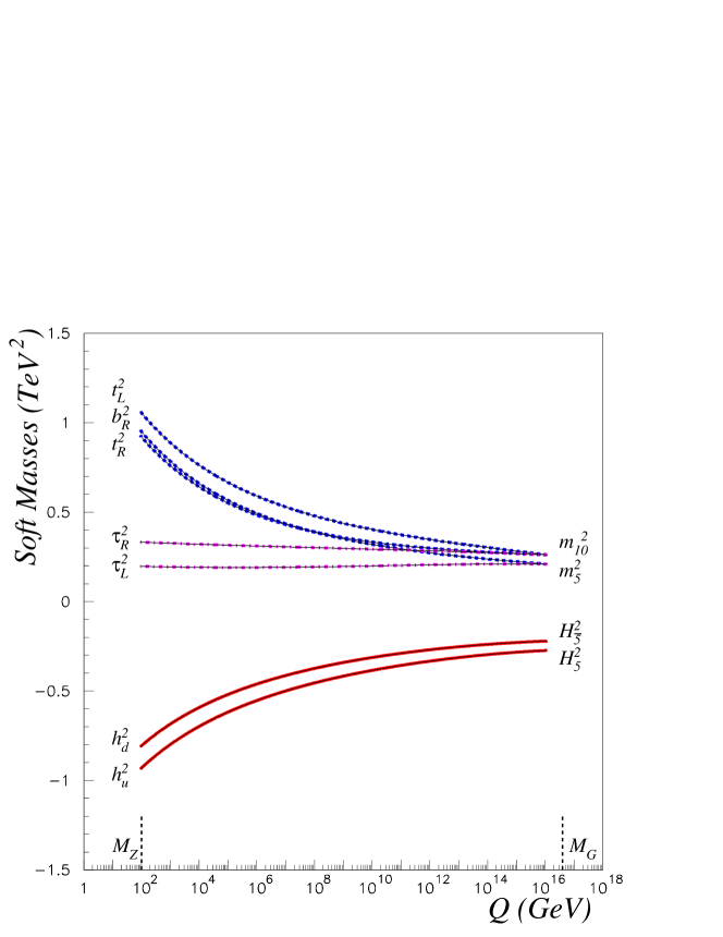
Figure 2: The two-loop evolution from unification to $M_{Z}$ scale of soft masses for the exact $SU(5)$ fixed point. The plot corresponds to point 1 in Table 6.

Analogously, fixed points for the soft masses will appear for the squared ratios of soft masses to the gaugino unified mass Lanzagorta:1995ai . The RGEs for these ratios in the minimal SU(5) model are given by

$$\frac{1}{g^{2}}\frac{d}{dt}\left(\begin{array}[]{c}\widetilde{m}_{5}^{2}\\ \widetilde{m}_{10}^{2}\\ \widetilde{m}_{{\cal H}_{5}}^{2}\\ \widetilde{m}_{{\cal H}_{\overline{5}}}^{2}\\ \widetilde{m}_{\Sigma}^{2}\end{array}\right)=\left({\cal M}\left(\begin{array}[]{c}\widetilde{m}_{5}^{2}\\ \widetilde{m}_{10}^{2}\\ \widetilde{m}_{{\cal H}_{5}}^{2}\\ \widetilde{m}_{{\cal H}_{\overline{5}}}^{2}\\ \widetilde{m}_{\Sigma}^{2}\end{array}\right)+{\cal N}\left(\begin{array}[]{c}\widetilde{A}_{t}^{2}\\ \widetilde{A}_{b}^{2}\\ \widetilde{A}_{H}^{2}\\ \widetilde{A}_{\Sigma}^{2}\end{array}\right)-\left(\begin{array}[]{c}48/5\\ 72/5\\ 48/5\\ 48/5\\ 20\end{array}\right)\right),$$ (33)

where we have defined

$$\widetilde{m}_{5}^{2}=\frac{m_{5}^{2}}{M^{2}_{1/2}},\qquad\widetilde{m}_{10}^{2}=\frac{m_{10}^{2}}{M^{2}_{1/2}},\qquad\widetilde{m}_{{\cal H}_{5}}^{2}=\frac{m_{{\cal H}_{5}}^{2}}{M^{2}_{1/2}},\qquad\widetilde{m}_{{\cal H}_{\overline{5}}}^{2}=\frac{m_{{\cal H}_{\overline{5}}}^{2}}{M^{2}_{1/2}},\qquad\widetilde{m}_{\Sigma}^{2}=\frac{m_{\Sigma}^{2}}{M^{2}_{1/2}},$$ (34)

and

$${\cal N}=\left(\begin{array}[]{cccc}0&4\widetilde{\lambda}_{b}^{2}&0&0\\ 3\widetilde{\lambda}_{t}^{2}&2\widetilde{\lambda}_{b}^{2}&0&0\\ 3\widetilde{\lambda}_{t}^{2}&0&24\widetilde{\lambda}_{H}^{2}/5&0\\ 0&4\widetilde{\lambda}_{b}^{2}&24\widetilde{\lambda}_{H}^{2}/5&0\\ 0&0&\widetilde{\lambda}^{2}_{H}&21\widetilde{\lambda}^{2}_{\Sigma}/20\end{array}\right),$$ (35)

$${\cal M}=\left(\begin{array}[]{ccccc}4\widetilde{\lambda}_{b}^{2}&4\widetilde{\lambda}_{b}^{2}&0&4\widetilde{\lambda}_{b}^{2}&0\\ 2\widetilde{\lambda}_{b}^{2}&6\widetilde{\lambda}_{t}^{2}+2\widetilde{\lambda}_{b}^{2}&3\widetilde{\lambda}_{t}^{2}&2\widetilde{\lambda}_{b}^{2}&0\\ 0&6\widetilde{\lambda}_{t}^{2}&3\widetilde{\lambda}_{t}^{2}+24\widetilde{\lambda}_{H}^{2}/5&24\widetilde{\lambda}_{H}^{2}/5&24\widetilde{\lambda}_{H}^{2}/5\\ 4\widetilde{\lambda}_{b}^{2}&4\widetilde{\lambda}_{b}^{2}&24\widetilde{\lambda}_{H}^{2}/5&4\widetilde{\lambda}_{b}^{2}+24\widetilde{\lambda}_{H}^{2}/5&24\widetilde{\lambda}_{H}^{2}/5\\ 0&0&\widetilde{\lambda}_{H}^{2}&\widetilde{\lambda}_{H}^{2}&\widetilde{\lambda}_{H}^{2}+63\widetilde{\lambda}_{\Sigma}^{2}/20\end{array}\right)-2b~{}{\cal I}_{5},$$ (36)

where ${\cal I}_{5}$ is the $5\times 5$ identity matrix. From Eq. (33) it is trivial to calculate the fixed point solution associated with the fixed point, Eq. (6), in the Yukawa sector:

$$\frac{m_{5}^{2}}{M^{2}_{1/2}}=\frac{436}{521},\quad\frac{m_{10}^{2}}{M^{2}_{1/2}}=\frac{545}{521},\quad\frac{m_{{\cal H}_{5}}^{2}}{M^{2}_{1/2}}=-\frac{569}{521},\quad\frac{m_{{\cal H}_{\overline{5}}}^{2}}{M^{2}_{1/2}}=-\frac{460}{521},\quad\frac{m_{\Sigma}^{2}}{M^{2}_{1/2}}=\frac{1550}{521}.$$ (37)

It can be easily proven that if the Yukawa couplings evolve towards the fixed point solution given by Eq. (6), the associated minimal SU(5) soft fixed point given by Eqs. (32) and (37) is stable Jack:1998xw . We already observed that the Yukawa fixed point, Eq. 6, in the direction $\lambda_{\Sigma}=0$ is not attractive. It is therefore crucial for the consistency of the soft-sector fixed point predictions that $\lambda_{\Sigma}$ be much smaller than the other dimensionless couplings. We also observe that the parameters $\mu_{H}$, $\mu_{\Sigma}$, $B_{H}$, and $B_{\Sigma}$ decouple from the rest of RGEs. To sum up, if we assume that the soft sector is at the fixed point associated with the fixed point in the Yukawa sector, the complete soft sector turns out to be strongly constrained. Therefore, we expect that definite predictions for the third generation supersymmetric spectra, as functions of the gaugino unified mass, will arise from the minimal SU(5) fixed point. In Fig. 2 we show the evolution of soft masses predicted by the fixed point for a representative value with $M_{1/2}=500$ GeV.

Let us add some qualitative comments regarding the uncertainty arising from the unknown ranges for the input conditions at a higher scale (Planck scale). When there is one dominant Yukawa coupling, one can address this question qualitatively. The rate of approach to the fixed point in this case is related to the coefficient $\left(\alpha_{s}(0)/\alpha_{s}(M_{P})\right)^{B}$, with $B=1+(r/b)$, where $b$ is the $\alpha_{s}$ beta coefficient and $r$ is the $\alpha_{s}$ coefficient in the Yukawa coupling RGE. The smaller this coefficient is, the faster the approach to the infrared fixed point is. In the minimal SUSY SU(5), $b=-3$ and $r=96/5$ and $84/5$ for the top and bottom-tau Yukawa couplings respectively. We can compare this case with the low $\tan(\beta)$ MSSM fixed point, where $r=16/3$ for the top Yukawa coupling. Since $\left(\alpha_{s}(0)/\alpha_{s}(M_{P})\right)>1$ and $B<0$ and approximately $8$ times larger in the minimal SUSY SU(5), we see that the coefficient is smaller in the minimal SUSY SU(5) than in the MSSM low tan(beta) fixed point scenario, i.e. the approach to the fixed point is faster in the minimal SUSY SU(5). Furthermore, we must keep in mind that in the case where several Yukawa couplings are of the same order, analytical approximations may not be reliable; a lengthy numerical study is required to determine the vessel attraction of the fixed point. We note, in favor of our main hypothesis, that the SU(5) fixed point predicts approximate universality for the sfermion soft masses, approximate top–bottom–tau Yukawa unification, and negative soft Higgs boson masses squared. It should be pointed out that many SUGRA models predict universality for the soft masses close to the Planck scale, and some string–inspired SUGRA models predict Yukawa unification. Observe that if we assume we have a SUGRA model at Planck scale with soft mass universality and top–bottom–tau Yukawa unification, then the initial conditions at Planck scale would already be very close to the SU(5) fixed point patterns, and the convergence to the fixed point at GUT scale could be much faster. With regard to the soft squared Higgs boson masses, even if these are positive at the Planck scale, they can be driven quickly to negative values at the GUT scale. This was observed in the analysis of the nonuniversalities in the SU(5) soft terms implemented by Polonsky and Pomarol (see Fig. 1 of Ref. pomarol ).

IV Unified fixed point and SU(5) breaking

The spontaneous symmetry breaking pattern is one of the non predictive aspects of grand unified models su5breaking . For the minimal supersymmetric SU(5), independent of the parameters of the scalar potential, there are many vacuum expectation values, all of which leave the supersymmetry unbroken. These break SU(5) spontaneously to smaller groups: SU(4)$\times$U(1), SU(3)$\times$SU(2)$\times$U(1), etc. A vacuum expectation value (VEV) with the desired breaking pattern to SU(3)$\times$SU(2)$\times$U(1) is among the possible vacua of the supersymmetric model

$$\left<\sigma\right>=\frac{\mu_{\Sigma}}{\lambda_{\Sigma}}\hbox{diag}\left(2,2,2,-3,-3\right).$$ (38)

This interesting VEV is degenerate in energy with a long list of physically unacceptable VEVs. To remove the degeneracy and to break supersymmetry, soft terms are added to the scalar potential. These terms have to be chosen with care to obtain a potential that remains bounded from below and leads to a VEV with the desired SU(5) breaking pattern. Certain relations between the scalar coupling constants of the Higgs multiplets have to be satisfied in order to have the SU(3)$\times$SU(2)$\times$U(1) minimum as the absolute minimum of the potential. In general, $m_{\Sigma}^{2}$ must be positive and small (relative to the GUT scale) for phenomenologically interesting symmetry breaking. One is thus led to take positive $m_{5}^{2}$ and $m_{10}^{2}$ to disfavor energetically all the solutions that involve nonvanishing VEVs for $\phi_{\overline{5}}$ and $\phi_{10}$ susysu5breaking . These two necessary conditions are satisfied at the SU(5) fixed point given by Eqs. (37).

It can be argued that some spontaneous symmetry breaking directions could be more natural than others if an infrared attractive fixed point is found within the corresponding region of Higgs parameter space Amelino-Camelia:1996ax ; amelino . The direction of SU(5) breaking determined by the vacuum expectation value $\left<\sigma\right>$ can be read off the scalar potential at the minimum

$${\cal V}^{{\rm min}}_{\rm SU(5)}=\rho M^{2}_{1/2}\left<\sigma\right>^{2}\left(\frac{m^{2}_{\Sigma}}{M^{2}_{1/2}}-\left[\frac{1}{3}\frac{A_{\Sigma}}{M_{1/2}}-2\frac{B_{\Sigma}}{M_{1/2}}\right]\frac{\lambda_{\Sigma}\left<\sigma\right>}{M_{1/2}}\right),$$ (39)

where $\rho=0$ for the minimum-preserving full SU(5) invariance, $\rho=30$ for the $G_{SM}=$ SU(3)$\times$SU(2)$\times$U(1) invariant minimum, and $\rho=20/9$ for the SU(4)$\times$U(1) invariant minimum. If ${\cal V}<0$ the $G_{SM}$ invariant minimum is the lowest one, while SU(5) remains unbroken if ${\cal V}>0$. If $\left|\lambda_{\Sigma}\right|<<\lambda_{t},\lambda_{b},\lambda_{H},g$, the fixed point predicts the ratios $m^{2}_{\Sigma}/M^{2}_{1/2}=1550/521$, and $A_{\Sigma}/M_{1/2}=-4650/521$.

The fixed point prediction for $B_{\Sigma}/M_{1/2}$ can be calculated from the RGE

$$\frac{1}{g^{2}}\frac{d}{dt}\left(\frac{B_{\Sigma}}{M_{1/2}}\right)=4\frac{A_{H}}{M_{1/2}}\frac{\lambda_{H}^{2}}{g^{2}}+\frac{84}{20}\frac{A_{\Sigma}}{M_{1/2}}\frac{\lambda_{\Sigma}^{2}}{g^{2}}+40+b\frac{B_{\Sigma}}{M_{1/2}}.$$ (40)

At the fixed point, given by Eqs. (6) and 32, $B_{\Sigma}/M_{1/2}=-6200/521=4A_{\Sigma}/3M_{1/2}$. In addition, the SU(5) spectrum includes 12 gauge bosons, $V=X,Y$, which receive a mass $M_{V}=5g\left<\sigma\right>\gtrsim M_{G}$, while $M_{1/2}$ determines the masses of the supersymmetric spectra. We therefore expect the ratio $\left<\sigma\right>/M_{1/2}$ to be approximately $10^{12-14}$ by phenomenological constraints. Therefore, the second or third terms are individually many orders of magnitude larger than the first term. As a consequence, the sign of the scalar potential is sensitive to the sign of $\lambda_{\Sigma}$, and we can only derive a constraint on $\lambda_{\Sigma}$ to obtain a satisfactory SU(5) breaking to the $G_{SM}$ invariant minimum

$${\cal V}^{{\rm min}}_{\rm SU(5)}<0\Longrightarrow\lambda_{\Sigma}>\frac{1}{3647}\frac{M_{1/2}}{\left<\sigma\right>}\simeq 3\times 10^{-16/-18}.$$

Thus, a correct SU(5) breaking is automatically achieved at the fixed point only for one sign of $\lambda_{\Sigma}$, positive in the convention used in this paper. We observe that the $\mu$-parameters, $\mu_{H}$ and $\mu_{\Sigma}$, remain undetermined at the fixed point.

It is, however, well known that in order for the Higgs SU(2) doublets to have masses of ${\cal O}(M_{Z})$ instead of ${\cal O}(M_{G})$, a fine tuning in the superpotential parameters is required, $\mu=(\mu_{H}+3\lambda_{H}\left<\sigma\right>)\simeq{\cal O}(M_{Z})$, and one obtains $\mu_{H}\simeq-3\sqrt{560/521}~{}g\left<\sigma\right>$ at the fixed point. Additionally, a fine tuning condition also arises in the soft sector, $B\mu=(B_{H}\mu_{H}+3A_{H}\lambda_{H}\left<\sigma\right>)\simeq{\cal O}(M_{Z}^{2})$, implying (using the first fine tuning condition) $B_{H}=A_{H}$. This condition is slightly different from the fixed point prediction for $B_{H}$, $B_{H}=4A_{H}/3$, even though it implies the same sign constraint on $\lambda_{\Sigma}$; this indicates a possible deviation from the fixed point prediction for the $B_{H}$ term. To complete the GUT spectra, we mention that the Higgs triplets receive a mass $M_{H_{C}}=5\lambda_{H}\left<\sigma\right>$, and the $\Sigma$ superfield decomposes with respect to ${\rm SU(3)}_{C}\times{\rm SU(2)}_{L}$ into $(3,2)+(\overline{3},2)+(8,1)+(1,3)+(1,1)$. In the supersymmetric limit the $(3,2)$ and $(\overline{3},2)$ are degenerate with the gauge bosons; the $(1,3)$ and $(8,1)$ components, $\Sigma_{3}$ and $\Sigma_{8}$, respectively, have a common mass $10\left|\mu_{\Sigma}\right|$; and the mass of the singlet, $\Sigma_{1}$, is $2\left|\mu_{\Sigma}\right|$. When soft breaking is considered, a boson-fermion mass splitting is induced within every multiplet.

V Electroweak breaking and supersymmetric spectra

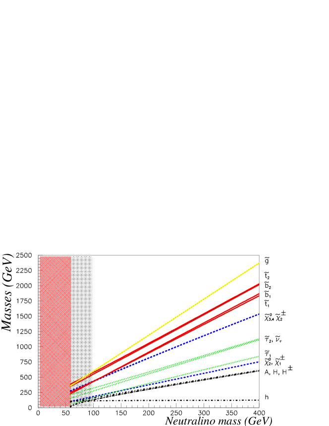
Figure 3: Low-energy superspectra from the exact SU(5) fixed point, Eqs. (42)-(45). The dark shaded region (red) is excluded by constraints on electroweak symmetry breaking, and the dot-shaded area (grey) is excluded by the experimental constraints on the Higgs mass.

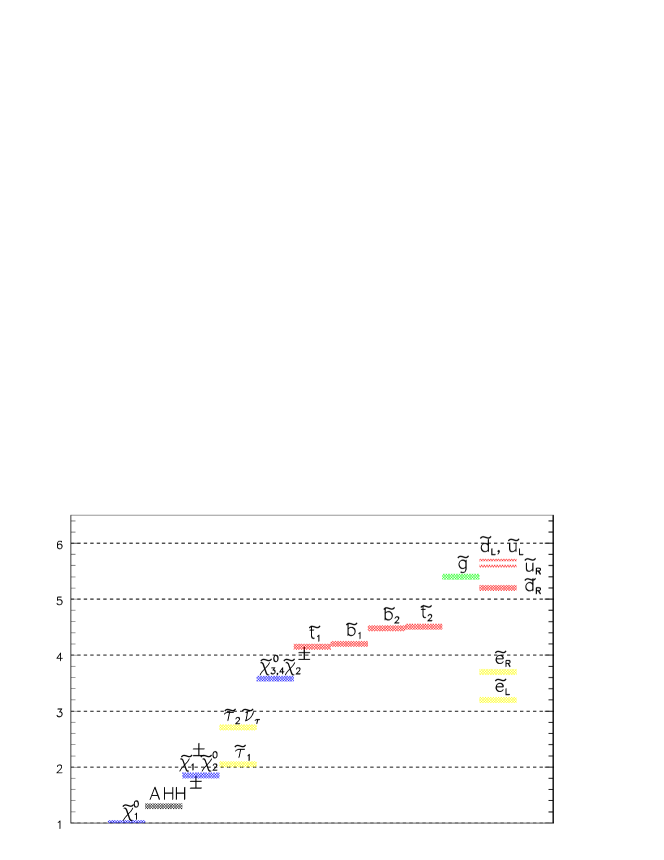
Figure 4: Characteristic ratios of masses for the low-energy superspectra from the exact SU(5) fixed point, Eqs. (42)-(45). The superspectra for the first and second generation masses are computed assuming the trivial fixed point of the SU(5) RGEs for the first and second generation soft parameters.

In order to analyze the implications of the SU(5) fixed point in the supersymmetric spectra, we have to run the MSSM RGEs from the GUT to the $m_{Z}$ scale. Below $M_{G}$ the effective theory is the third generation MSSM defined by the superpotential given in Eq. (10). The associated soft scalar potential is given by

$${\cal V}^{\rm soft}_{\rm MSSM} = m^{2}_{H_{d}}\left|{h}_{d}\right|^{2}+m^{2}_{H_{u}}\left|{h}_{u}\right|^{2}+\frac{1}{2}\left[\sum_{i=1,3}M_{i}\lambda_{i}\lambda_{i}+B\mu h_{u}h_{d}+{\cal{\rm h.c.}}\right]$$ (41)

$$+m^{2}_{\widetilde{b}_{L}}\left|\widetilde{b}_{L}\right|^{2}+m^{2}_{\widetilde{b}_{R}}\left|\widetilde{b}_{R}\right|^{2}+m^{2}_{\widetilde{t}_{L}}\left|\widetilde{t}_{L}\right|^{2}+m^{2}_{\widetilde{t}_{R}}\left|\widetilde{t}_{R}\right|^{2}+m^{2}_{\widetilde{\tau}_{R}}\left|\widetilde{\tau}_{R}\right|^{2}+m^{2}_{\widetilde{\tau}_{L}}\left|\widetilde{\tau}_{L}\right|^{2}$$

$$+\left[A_{t}h_{t}\widetilde{t}_{L}{h}_{u}\widetilde{t}_{R}+A_{b}h_{b}\widetilde{t}_{L}{h}_{d}\widetilde{b}_{R}+A_{\tau}h_{\tau}\widetilde{\tau}_{L}{h}_{d}\widetilde{\tau}_{R}+{\cal{\rm h.c.}}\right].$$

The soft parameters are determined at $M_{G}$ by the boundary conditions given by the SU(5) fixed point at the unification scale, Eqs. (32) and (37)

$$m^{2}_{\widetilde{t}_{L},\widetilde{t}_{R},\widetilde{b}_{L},\widetilde{\tau}_{R}} = \frac{545}{521}~{}M^{2}_{1/2},$$ (42)

$$m^{2}_{\widetilde{b}_{R},\widetilde{\tau}_{L},\widetilde{\nu}_{\tau}} = \frac{436}{521}~{}M^{2}_{1/2},$$ (43)

$$m_{{\cal H}_{u}}^{2}=-\frac{569}{521}~{}M^{2}_{1/2} < m_{{\cal H}_{d}}^{2}=-\frac{460}{521}~{}M^{2}_{1/2},$$ (44)

$$A_{t,b,\tau} = -M_{1/2}.$$ (45)

The bilinear parameters $\mu$ and $B$ are not determined by the fixed point. They must be computed from the MSSM minimization equations under the constraint of a correct electroweak symmetry breaking at $m_{Z}$. In this scenario, as in generic supersymmetric unified scenarios, we do not know why $m_{Z}$ is many orders of magnitude smaller than $M_{G}$; equivalently, the MSSM $\mu$-term must be many orders of magnitude smaller than $M_{G}$. Many possible solutions have been proposed in the literature in the context of non minimal models Kim:1983dt .

Let us describe in more detail the numerical procedure followed in this paper to minimize the MSSM scalar potential. Once we assume some GUT scale initial conditions resulting from the SU(5) fixed point we use the complete set of MSSM RGEs (two loop for dimensionless couplings and main two loop contributions for dimensionful couplings) to extrapolate the MSSM couplings to the electroweak scale. Next we use the experimental value of the tau mass and the tau Yukawa coupling at $m_{Z}$ (from the RGEs) to determine $\tan(\beta)$ at tree level using Eq. (14). We use then the tree level minimization equations and the running couplings at $m_{Z}$, obtained from the RGEs, to compute the parameters $\mu$ and $B\mu$ (this is the optimal choice since the bilinear parameters are decoupled from the rest of RGEs), then we compute the tree level supersymmetric spectra. Then we do a second iteration. Using the effective potential we implement the one–loop minimization of the scalar potential including corrections coming from sfermion loops Arnowitt:qp , and we also include one loop SUSY threshold corrections in the relation between third fermion masses and Yukawa couplings. Once we have included one loop corrections we compute again $\tan\beta$, $\mu$, $B\mu$ and the superspectra. We do several more iterations until the results converge. In this way the correct minimization of the MSSM, compatible with the large value of $\tan(\beta)$ fixed by the tau mass, is guaranteed.

We point out that the SU(5) fixed point boundary conditions allow us to obtain a satisfactory tree-level electroweak symmetry breaking. This is a non trivial fact that is quite simple to understand by a tree level analysis. Even though the $\mu$-term and the $CP$-odd Higgs boson mass, $m_{A}$, receive important radiative contributions, their main contribution is the tree-level one. From the MSSM minimization equations, $m_{A}$ is given at tree level by

$$m_{A}^{2}=\left(\frac{t^{2}_{\beta}+1}{t^{2}_{\beta}-1}\right)\left(m_{H_{d}}^{2}-m_{H_{u}}^{2}\right)-M_{Z}^{2}.$$ (46)

The fixed point predicts $h_{t}(M_{G})>h_{b}(M_{G})$ and

$$m_{H_{d}}^{2}(M_{G})-m_{H_{u}}^{2}(M_{G})=\frac{109}{521}M_{1/2}^{2}>0.$$ (47)

The structure of the MSSM RGEs keeps the difference $(m_{H_{d}}^{2}-m_{H_{u}}^{2})$ positive from the GUT to the $M_{Z}$ scale. As a consequence, a satisfactory tree-level electroweak symmetry breaking is possible if the gaugino mass is large enough. In Fig. 3 we plot the spectra as a function of the neutralino mass. Numerically we find that in order to achieve electroweak symmetry breaking we must have $m_{\chi^{0}_{1}}>50$ GeV, corresponding to the constraint $M_{1/2}\gtrsim 145$ GeV. The region excluded by this constraint is shown by the dark shaded (red) area in Fig. 3. On the other hand, the experimental measurement of the tau lepton mass implies that the fixed point is phenomenologically viable only when $\tan\beta$ is large. At such a limit the $\mu$-term is given at tree level by

$$\mu^{2}\simeq-m_{H_{u}}^{2}-\frac{1}{2}M^{2}_{Z}>0.$$ (48)

Therefore, $\mu^{2}$ is automatically positive if $M_{1/2}$ (and hence -$m_{H_{u}}^{2}$) is large enough, because the fixed point predicts $m_{H_{u}}^{2}<0$. This bound on $M_{1/2}$ is milder than the constraint derived from the condition $m^{2}_{A}>0$. Since the soft parameters are proportional to $M_{1/2}$ , sparticle masses are to a good approximation also proportional to the unified gaugino mass. This characteristic can be clearly observed in Fig. 3. For a neutralino mass $m_{\chi^{0}_{1}}\lesssim 100$ GeV, the fixed point predicts a Higgs boson experimentally excluded, $m_{h}<114$ GeV (see grey area in Fig. 3). The Higgs boson masses have been computed including one loop sfermion corrections MSSMeffective , while the other masses have been computed at tree level. As can be seen in Fig. 3, a clear mass pattern arises, the SUSY-QCD sector being the heaviest:

$$m_{\widetilde{g}}>m_{\widetilde{t}_{2}}\simeq m_{\widetilde{b}_{2}}>m_{\widetilde{b}_{1}}\gtrsim m_{\widetilde{t}_{1}}.$$

The lightest neutralino, $m_{\chi^{0}_{1}}$, is mostly B-ino. The heavier chargino and the two heaviest neutralinos are mostly Higgsinos, and form an approximately degenerate singlet, $\widetilde{\chi}^{0}_{3}$, and triplet, $(\widetilde{\chi}^{+}_{2},\widetilde{\chi}^{0}_{4},\widetilde{\chi}^{-}_{2})$, of ${\rm SU(2)}_{L}$, all with masses set by the $\mu$-parameter. The second lightest neutralino and the lightest chargino are mostly W-inos and form a degenerate triplet of ${\rm SU(2)}_{L}$, $(\widetilde{\chi}^{+}_{1},\widetilde{\chi}^{0}_{2},\widetilde{\chi}^{-}_{1})$. The following mass pattern arises:

$$m_{\widetilde{\chi}^{0}_{3,4}}\simeq m_{\widetilde{\chi}^{\pm}_{2}}>m_{\widetilde{\tau}_{2}}\simeq m_{\widetilde{\nu}_{\tau}}>m_{\widetilde{\tau}_{1}}>m_{\widetilde{\chi}^{0}_{2}}\simeq m_{\widetilde{\chi}^{\pm}_{1}}>m_{A}\simeq m_{H}\simeq m_{H}^{\pm}.$$

The fixed point does not only predict qualitative relations between the masses of the supersymmetric spectra. Except for $m_{h}$, the ratios of masses are more or less fixed, as shown in Fig. 4:

$$\left(m_{\widetilde{g}},m_{\widetilde{t}_{2},\widetilde{b}_{2}},m_{\widetilde{b}_{1}},m_{\widetilde{t}_{1}}\right) \simeq \left(5.5,~{}4.7,~{}4.4,~{}4.2\right)\times m_{\widetilde{\chi}^{0}_{1}},$$ (49)

$$\left(m_{\widetilde{\chi}^{\pm}_{2},\widetilde{\chi}^{0}_{3,4}},m_{\widetilde{\tau}_{2},\widetilde{\nu}_{\tau}},m_{\widetilde{\tau}_{1}},m_{\widetilde{\chi}^{\pm}_{1},\widetilde{\chi}^{0}_{2}}\right) \simeq \left(2.9,~{}2.5,~{}2.2,~{}1.8\right)\times m_{\widetilde{\chi}^{0}_{1}},$$ (50)

$$m_{A,H,H^{\pm}} \simeq 1.34\times m_{\widetilde{\chi}^{0}_{1}}.$$ (51)

Since $m^{2}_{\tilde{t}_{L}}\simeq m^{2}_{\tilde{t}_{R}}\simeq m^{2}_{\tilde{b}_{R}}$ and $m^{2}_{\tilde{\tau}_{L}}\simeq m^{2}_{\tilde{\tau}_{R}}$, the diagonal entries of the sfermion matrices are very similar, and the sfermion mixing is quasimaximal.

In summary, the fixed point (a) is compatible with a correct electroweak symmetry breaking if $M_{1/2}\gtrsim 150$ GeV, (b) predicts the neutralino as the LSP for all the allowed parameter space, and (c) predicts definite relations between the masses of the superspectra (see Fig. 4). These mass relations could give us a clear confirmation of the SU(5) fixed point scenario in future experiments, once several supersymmetric particles have been observed.

VI top and bottom mass predictions including one-loop supersymmetric thresholds

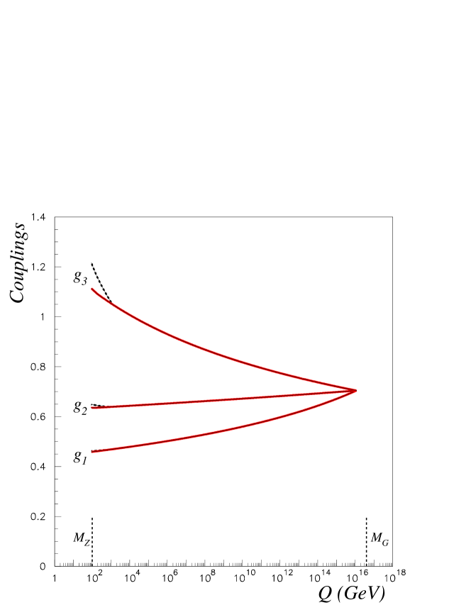
Figure 5: Gauge coupling running at two-loop (solid red line) in the MSSM from the GUT to the $M_{Z}$ scale, plus one-loop logarithmic SUSY thresholds (black dashed line). The plot corresponds to the point 1 in Table 6.

Once we know the supersymmetric spectra predicted by the SU(5) fixed point, we can refine the predictions for gauge couplings and for top and bottom quark masses, including the low-energy supersymmetric threshold corrections. Incorporating these is the main purpose of this section. We begin with a description of our numerical procedure for implementing these thresholds.

VI.1 Low-energy supersymmetric thresholds

Assuming a common decoupling scale for all the supersymmetric particles, the logarithmic SUSY threshold corrections to the strong coupling constant $\alpha_{s}(M_{Z})$ would be given by a simple formula loggaug :

$$\alpha_{s}^{\rm SM}(m_{Z})=\frac{\alpha_{s}^{\rm MSSM}(m_{Z})}{1-\frac{2\alpha_{s}^{\rm MSSM}(m_{Z})}{\pi}\ln\left(\frac{M_{\rm SUSY}}{m_{Z}}\right)}>\alpha_{s}^{\rm MSSM}(m_{Z}).$$ (52)

We observe that in general the supersymmetric thresholds increase the value of $\alpha^{\rm SM}_{s}(M_{Z})$ with respect to the MSSM prediction. In our study, the logarithmic thresholds to the three gauge couplings have been implemented numerically, decoupling one by one the supersymmetric particles from the one-loop beta functions in the integration of the renormalization group equations from the GUT to the $M_{Z}$ scale. The effect of the supersymmetric thresholds on the gauge couplings is shown in Fig. 5 (dashed black line) for one representative point of our scans. The solid-red line corresponds to the two-loop MSSM gauge coupling running with no thresholds. The effect of the thresholds is crucial for a precise prediction of $\alpha_{s}$, $\widehat{\alpha}_{em}$ and $\widehat{s}^{2}_{W}$ gaugeunif ; loggaug . The thresholds to $\alpha_{1}$ and $\alpha_{2}$ are smaller but no less important, due to the small uncertainty in their experimental measurement.

The physical top quark mass is calculated from the expression

$$m_{t}=h_{t}(m_{t})v(m_{t})s_{\beta}\left(1+\Delta_{\rm QCD}^{\rm t}+\Delta_{\rm SUSY}^{\rm t}\right),$$ (53)

where $\Delta_{\rm QCD}^{\rm t}$ stands for the gluon correction that was given in Eq. (22), and $\Delta_{\rm SUSY}^{t}$ is the supersymmetric contribution evaluated at $m_{t}$ scale. $\Delta_{\rm SUSY}^{t}$ includes contributions from all the third generation MSSM spectra. We have implemented the complete one-loop contributions to $\Delta_{\rm SUSY}^{t}$ as given in Ref. Pierce:1996zz . A posteriori, we observe that the dominant contribution to $\Delta^{t}_{\rm SUSY}$ is the logarithmic component of the gluino-stop diagrams, $\Delta^{t}_{\widetilde{g}-{\rm Log}}$, which is in general positive for $m_{\widetilde{g}}>m_{t}$. This contribution is

$$\Delta^{t}_{\widetilde{g}-{\rm Log}}=\frac{1}{3}\frac{\alpha_{s}(m_{t})}{\pi}\left[\ln\left(\frac{m_{\widetilde{g}}^{2}}{m^{2}_{t}}\right)-\frac{1}{2}+\sum_{i=1,2}g(x_{\widetilde{t}_{i}})\right],$$ (54)

where $x_{\widetilde{t}_{1,2}}=m^{2}_{\widetilde{t}_{1},\widetilde{t}_{2}}/m^{2}_{\widetilde{g}}$, and the function $g(x)$ is given by

$$g(x)=\frac{1}{2}\left[\ln x-\frac{1}{1-x}-\frac{\ln x}{(1-x)^{2}}\right].$$ (55)

This function satisfies $\left|g(x)\right|<1/2$ if $0<x<1$ and $g(1)=1/4$. At the fixed point, using the predicted ratios for the SUSY spectra given in Eq. (49), a simple expression for this contribution can be written, which works as a very good approximation:

$$\left(\Delta^{t}_{\widetilde{g}-{\rm Log}}\right)_{{\rm SU(5)f.p.}}\simeq\frac{1}{3}\frac{\alpha_{s}(m_{t})}{\pi}\left[\ln\left(\frac{m_{\widetilde{g}}^{2}}{m^{2}_{t}}\right)-\frac{1}{4}\right].$$ (56)

The standard model running bottom quark mass just above $m_{Z}$ in the $\overline{\rm DR}$ scheme is computed using the formula

$$m_{b}^{\overline{\rm DR}}(m_{Z}^{>})=h_{b}(m_{Z})v(m_{Z})\cos\beta\left(1+\Delta_{\rm SUSY}^{b}\right),$$ (57)

where $m_{b}^{\overline{\rm DR}}(m_{Z}^{>})$ is related to $m_{b}^{\overline{\rm MS}}(m_{Z}^{<})$, the running mass just below $m_{Z}$, as explained in Sect. II. $\Delta_{\rm SUSY}^{b}$ is the supersymmetric threshold evaluated at the $m_{Z}$ scale. $\Delta_{\rm SUSY}^{b}$ includes contributions from all the third generation MSSM spectra. We have implemented the complete one-loop expressions given in Ref. Pierce:1996zz . We observe that there are three dominant contributions to $\Delta_{\rm SUSY}^{b}$: the logarithmic, $\Delta^{b}_{\widetilde{g}-{\rm Log}}$, and finite, $\Delta^{b}_{\widetilde{g}-{\rm Fin}}$, pieces of the gluino-sbottom diagram and the chargino-stop contribution, $\Delta^{b}_{\widetilde{\chi}-\widetilde{t}}$. These are given below. The logarithmic part of the gluino-sbottom contribution is analogous to the gluino-stop contribution to the top mass:

$$\Delta^{b}_{\widetilde{g}-{\rm Log}}=\frac{1}{3}\frac{\alpha_{s}(m_{Z})}{\pi}\left[\ln\left(\frac{m_{\widetilde{g}}^{2}}{m^{2}_{Z}}\right)-\frac{1}{2}+\sum_{i=1,2}g(x_{\widetilde{b}_{i}})\right].$$ (58)

At the fixed point, there is a simpler formula analogous to Eq. (56)

$$\left(\Delta^{b}_{\widetilde{g}-{\rm Log}}\right)_{{\rm SU(5)f.p.}}\simeq\frac{1}{3}\frac{\alpha_{s}(m_{Z})}{\pi}\left[\ln\left(\frac{m_{\widetilde{g}}^{2}}{m^{2}_{Z}}\right)-\frac{1}{4}\right],$$ (59)

which also works as a very good approximation. The finite part of the gluino-sbottom contribution is given at large $\tan\beta$ by

$$\Delta^{b}_{\widetilde{g}-{\rm Fin}}=\frac{2}{3}\frac{\alpha_{s}(m_{Z})}{\pi}\frac{\mu t_{\beta}}{m_{\widetilde{g}}}f(x_{\widetilde{b}_{1}},x_{\widetilde{b}_{2}}),$$ (60)

with $x_{\widetilde{b}_{1,2}}=m^{2}_{\widetilde{b}_{1,2}}/m_{\widetilde{g}}^{2}$ and $m_{\widetilde{b}_{2}}>m_{\widetilde{b}_{1}}$. The function $f(x,y)$ is given by

$$f(x,y)=\frac{\left[(1-y)x\ln x-(1-x)y\ln y\right]}{(y-x)(1-x)(1-y)},$$ (61)

where $f(x_{\widetilde{b}_{1}},x_{\widetilde{b}_{2}})>0$. Therefore, the sign of $\Delta^{b}_{\widetilde{g}-{\rm Fin}}$ is the sign of the $\mu$-term. Moreover, the ratios $x_{\widetilde{b}_{1,2}}$ are well determined by the SU(5) fixed point predictions, $x_{\widetilde{b}_{1}}\simeq 0.61$ and $x_{\widetilde{b}_{1}}\simeq 0.74$. We thus obtain $f(x_{\widetilde{b}_{1}},x_{\widetilde{b}_{2}})\simeq 16/25$, so that to a very good approximation,

$$\left(\Delta^{b}_{\widetilde{g}-{\rm Fin}}\right)_{{\rm SU(5)f.p.}}\simeq\frac{32}{75}\frac{\alpha_{s}(m_{Z})}{\pi}\frac{\mu t_{\beta}}{m_{\widetilde{g}}}.$$ (62)

At large $\tan\beta$, the dominant contribution to the chargino-stop diagram is given by

$$\Delta^{b}_{\widetilde{\chi}-\widetilde{t}}\simeq\frac{h^{2}_{t}}{16\pi^{2}}\frac{A_{t}t_{\beta}}{\mu}f(x_{\widetilde{t}_{1}},x_{\widetilde{t}_{1}}),$$ (63)

where $x_{\widetilde{t}_{1,2}}=m^{2}_{\widetilde{t}_{1,2}}/\mu^{2}$. The fixed point predicts $m_{\widetilde{t}_{2}}>m_{\widetilde{t}_{1}}>\left|\mu\right|$ and, in general, $A_{t}<0$. Thus, the sign of this contribution is inversely correlated with the sign of $\mu$. The standard model running tau mass just above $m_{Z}$ is computed using the formula

$$m_{\tau}(m_{Z}^{>})=h_{\tau}(m_{Z})v(m_{Z})\cos\beta\left(1+\Delta_{\rm SUSY}^{\tau}\right),$$ (64)

where $m_{\tau}(m_{Z}^{>})$ is related to the running mass just below $m_{Z}$ as explained in Sect. II. $\Delta_{\rm SUSY}^{\tau}$ implements the complete one-loop supersymmetric threshold evaluated at the $m_{Z}$ scale Pierce:1996zz . We observe that there is a dominant contribution to $\Delta_{\rm SUSY}^{\tau}$, the chargino loop given by

$$\Delta^{\tau}_{\widetilde{\chi}^{\pm}-\widetilde{\nu}_{\tau}}=-\frac{\alpha_{2}(m_{Z})}{4\pi}\frac{M_{2}t_{\beta}}{\mu}f(x_{M_{2}},x_{\widetilde{\nu}_{\tau}}),$$ (65)

where $x_{M_{2}}=M_{2}^{2}/\mu^{2}$ and $x_{\widetilde{\nu}_{\tau}}=m^{2}_{\widetilde{\nu}_{\tau}}/\mu^{2}$. As a result, $f(x_{M_{2}},x_{\widetilde{\nu}_{\tau}})>0$, and $\Delta^{\tau}_{\widetilde{\chi}^{\pm}-\widetilde{\nu}_{\tau}}$ is inversely correlated with the sign of $\mu$. The fixed point predicts $\left|\mu\right|>m_{\widetilde{\nu}_{\tau}}>M_{2}$, and since $\alpha_{2}(m_{Z})$ is approximately $0.03$, we expect this contribution to be much smaller than the chargino-stop contribution to the bottom mass. We obtain typically $\Delta^{\tau}_{\widetilde{\chi}^{\pm}-\widetilde{\nu}_{\tau}}\simeq+4\%$ to $+6\%$ for $\mu<0$ and $-4\%$ to $-6\%$ for $\mu>0$, which turns out to be important for a precise determination of $\tan\beta$.

VI.2 Mass spectra: numerical results

The complete SU(5) fixed point scenario contains four parameters: $M_{G}$, $g$, $M_{1/2}$, and $\tan\beta$. The numerical procedure that we will use in this case is a generalization of the procedure we used in Sect. II for the case with no supersymmetric thresholds. We first scan the model parameter space $(M_{G},g)$ for different values of $M_{1/2}$ and integrate numerically the complete set of two-loop MSSM RGEs from the GUT to the $m_{Z}$ scale. We next compute the low-energy supersymmetric spectra and supersymmetric thresholds to gauge couplings, and consider only those solutions that fix the experimental values of $\alpha_{s}(m_{Z})_{\overline{\rm MS}}$ and $\alpha_{e}^{-1}(m_{Z})_{\overline{\rm MS}}$. Then we use the measured value of the tau mass and Eq. (64) to fix $\tan\beta$. Once we know $\tan\beta$, we can compute the thresholds to the fermion masses. Finally, we obtain three predictions for $m_{t}$, $m_{b}(m_{Z})_{\overline{\rm MS}}$, and $\widehat{s}^{2}_{W}(m_{Z})_{\overline{\rm MS}}$.

Since threshold corrections to fermion masses depend on the sign of $\mu$, we must distinguish two cases: $\mu<0$, for which results are shown in Table 4, and $\mu>0$, for which results are shown in Table 5. We begin with four choices of $M_{1/2}$: $250,500,1000$, and $1500$ GeV. We show in Tables 4 and 5 our theoretical predictions for $\widehat{s}^{2}_{W}(M_{Z})_{\overline{\rm MS}}$, $m_{b}(m_{Z})_{\overline{\rm MS}}$, $m_{t}$, the Higgs boson mass $h$, and the LSP (lightest supersymmetric particle), along with the values of the input parameters $M_{G}$, $g$ and $\tan\beta$. The following points are worth noting

• The top mass is predicted to be well within the experimental range, $m_{t}\simeq 174.3\pm 5.1$ GeV. Moreover, its predicted value turns out to be only weakly sensitive to $M_{1/2}$ and the sign of $\mu$, ranging between $174.4$ GeV and $176.9$ GeV, as shown in Fig. 6.

• It is well known that predictions for the weak mixing angle in supersymmetric unified models, with SUSY spectra below $2$ TeV, are not completely successful but still very good. It is important to keep in mind that according to PDG $\widehat{s}^{2}_{W}(M_{Z})_{\overline{\rm MS}}=0.23117(16)$, thus $\sigma$, the experimental uncertainty, is only $0.07\%$. Our model predicts that for $M_{1/2}=250$ GeV, the central value for $\widehat{s}^{2}_{W}(M_{Z})_{\overline{\rm MS}}$ is $0.2338$, which is more than $+16~{}\sigma$ away from the experimental value; and for $M_{1/2}=1.5$ TeV, our central value is $0.2322$ which is at $+6~{}\sigma$. In spite of this, it must be considered a good prediction since, if we take into account that the experimental uncertainty, we predict the weak mixing angle correctly below $1\%$ precision.

• The prediction for the bottom mass is very sensitive to the sign of $\mu$ and to the unified gaugino mass. For $\mu>0$, our predicted value is clearly too large. For $\mu<0$, it is uncomfortably small but gets close to its experimental value, $m_{b}^{\overline{\rm MS}}(m_{Z}^{>})=2.86\pm 0.2$ GeV, for large values of the gaugino mass, as shown in Fig. 8. We will focus on $\mu<0$ below.

• The higher the gaugino unified mass, the lower the gauge unified coupling, and the lower the unification scale. This is because the thresholds on the value of the gauge couplings at $m_{Z}$, are always positive, as can be seen in Eq. (52) and Fig. 5, and they increase with the gaugino mass. Numerically, we find that for $\alpha_{s}$ the threshold corrections are $\sim 19\%$.

parameters	A	B	C	D
$M_{1/2}$ (GeV)	$250$	$500$	$750$	$1500$
experimental constraints
$\alpha_{e}(m_{Z})^{-1}_{\overline{\rm MS}}$	$127.934\pm 0.027$
$\alpha_{s}(m_{Z})_{\overline{\rm MS}}$	$0.1172\pm 0.0020$
$m_{\tau}$ (GeV)	$1.77703$
model parameters
$M_{G}\times 10^{-16}$ (GeV)	$1.205\pm 0.139$	$1.130\pm 0.126$	$1.074\pm 0.020$	$0.9995\pm 0.1122$
$\alpha_{G}^{-1}$	$0.7094\pm 0.001$	$0.7037\pm 0.0011$	$0.7005\pm 0.0011$	$0.6951\pm 0.0011$
$\tan\beta$	$51.74\pm 0.03$	$51.626\pm 0.02$	$51.62\pm 0.02$	$50.569\pm 0.056$
theoretical predictions
$s_{W}^{2}(m_{Z})_{\overline{\rm MS}}$	$0.2338\pm 0.0005$	$0.2332\pm 0.0005$	$0.2328\pm 0.0005$	$0.2322\pm 0.0005$
$m_{t}$ (GeV)	$176.01\pm 0.97$	$175.67\pm 1.06$	$175.39\pm 1.08$	$174.401\pm 1.06$
$m_{b}(m_{Z})_{\overline{\rm MS}}$ (GeV)	$2.023\pm 0.005$	$2.159\pm 0.006$	$2.215\pm 0.008$	$2.376\pm 0.010$
$m_{h}$ (GeV)	$113.85\pm 0.14$	$119.09\pm 0.06$	$121.32\pm 0.04$	$123.362\pm 0.03$
$m_{\chi^{0}_{1}}$ (GeV)	$101.43\pm 0.47$	$206.67\pm 0.92$	$312.58\pm 1.35$	$632.98\pm 2.74$

Table 4: Predictions from a minimal supersymmetric SU(5) exact fixed point, including low-energy supersymmetric threshold corrections, for $M_{1/2}<1.5$ TeV and $\mu<0$.

parameters	A	B	C	D
$M_{1/2}$ (GeV)	$250$	$500$	$1000$	$1500$
experimental constraints
$\alpha_{e}(m_{Z})^{-1}_{\overline{\rm MS}}$	$127.934\pm 0.027$
$\alpha_{s}(m_{Z})_{\overline{\rm MS}}$	$0.1172\pm 0.0020$
$m_{\tau}$ (GeV)	$1.77703$
model parameters
$M_{G}\times 10^{-16}$ (GeV)	$1.205\pm 0.139$	$1.130\pm 0.126$	$1.074\pm 0.121$	$0.9995\pm 0.112$
$\alpha_{G}^{-1}$	$0.7094\pm 0.001$	$0.7038\pm 0.0011$	$0.700\pm 0.001$	$0.6951\pm 0.001$
$\tan\beta$	$43.727\pm 0.015$	$43.460\pm 0.012$	$44.05\pm 0.012$	$43.836\pm 0.02$
theoretical predictions
$s_{W}^{2}(m_{Z})_{\overline{\rm MS}}$	$0.2338\pm 0.0005$	$0.2332\pm 0.0005$	$0.2328\pm 0.0005$	$0.2322\pm 0.0005$
$m_{t}$ (GeV)	$176.03\pm 0.97$	$175.70\pm 1.06$	$175.14\pm 1.08$	$174.42\pm 1.06$
$m_{b}(m_{Z})_{\overline{\rm MS}}$ (GeV)	$4.436\pm 0.04$	$4.335\pm 0.04$	$4.216\pm 0.040$	$4.139\pm 0.038$
$m_{h}$ (GeV)	$114.56\pm 0.11$	$119.40\pm 0.073$	$121.58\pm 0.04$	$123.55\pm 0.03$
$m_{\chi^{0}_{1}}$ (GeV)	$101.01\pm 0.45$	$206.30\pm 0.92$	$312.443\pm 1.349$	$632.256\pm 2.63$

Table 5: Predictions from a minimal supersymmetric SU(5) exact fixed point, including low-energy supersymmetric threshold corrections, for $M_{1/2}<1.5$ TeV and $\mu>0$.

VI.3 Predictions for multi-TeV gaugino mass and naturalness

In light of the successful top-quark-mass prediction of the SU(5) fixed point scenario, one is compelled to consider extreme possibilities, which, surprising as it may seem, could allow the fixed point to predict correctly the bottom mass and the weak mixing angle. The alert reader may have realized (see Table 4) that for large gaugino unified mass and $\mu<0$, not only does the bottom mass approach its experimental value, but the prediction for the weak mixing angle also approaches its experimentally measured value.

In Table  6, we extend the range of study of our model to multi-TeV gaugino unified masses. We show all the parameters and spectra for five representative points, with $M_{1/2}=0.5,1.5,5,7$ and $10$ TeV. We observe that the bottom mass prediction increases continuously with $M_{1/2}$, going from $2.16$ GeV for $M_{1/2}=500$ GeV to $2.56$ GeV for $M_{1/2}=10$ TeV, as shown Fig. 8. We observe also that the predictions for the weak mixing angle are good in this range: the weak mixing angle is $0.23121$ for $M_{1/2}=5$ TeV, which is inside the $1~{}\sigma$ experimental window, $0.23092$ for $M_{1/2}=7$ GeV, which is inside the $-2~{}\sigma$ experimental window, and $0.23061$ for $M_{1/2}=10$ TeV, which is inside the $-4~{}\sigma$ experimental window. In Fig. 7 we plot the weak mixing angle as a function of the gaugino mass. We also show in Fig. 6 the stability of the top mass prediction in this scenario for very large gaugino masses as a function of the gaugino mass.

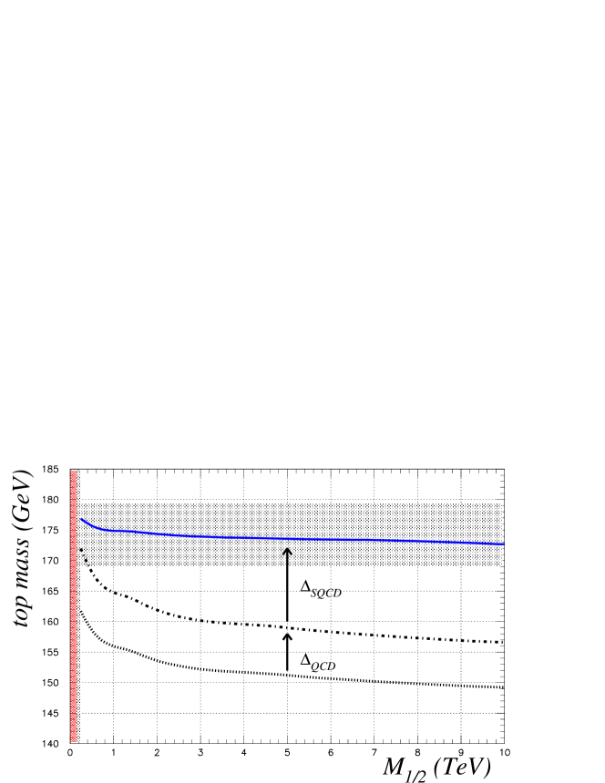
Figure 6: Top mass prediction from the minimal supersymmetric SU(5) exact fixed point with $\mu<0$ as a function of the gaugino mass. The shaded area represents the experimental world average.

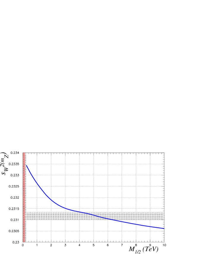
Figure 7: Weak mixing angle prediction from a minimal supersymmetric SU(5) exact fixed point, with $\mu<0$, as a function of the gaugino mass. The shaded area represents the experimentally allowed region.

parameters	point-1	point-2	point-3	point-4	point-5
model parameters
$M_{1/2}$ (TeV)	$0.5$	$1.5$	$5$	$7$	$10$
$M_{G}\times 10^{-16}$ (GeV)	1.12640	0.99135	0.86852	0.83742	0.81275
$g$	0.70386	0.69517	0.68609	0.68359	0.68101
$\tan\beta$	51.65211	51.311	51.055	50.91695	50.74379
MSSM Yukawa couplings at $M_{G}$
$h_{t}(M_{G})$	0.69406	0.68549	0.67654	0.67408	0.67153
$h_{b}(M_{G})$	0.53250	0.52593	0.51906	0.51717	0.51521
$h_{\tau}(M_{G})$	0.53250	0.52593	0.51906	0.51717	0.51521
MSSM dimensionless couplings at $M_{Z}$
$g_{1}(M_{Z})$	0.45845	0.45659	0.45456	0.45399	0.45337
$g_{2}(M_{Z})$	0.63462	0.62870	0.62241	0.62067	0.61885
$g_{3}(M_{Z})$	1.11336	1.07751	1.04229	1.03298	1.02373
$h_{t}(M_{Z})$	0.92405	0.90163	0.87937	0.87343	0.86745
$h_{b}(M_{Z})$	0.80753	0.78475	0.76220	0.75620	0.75018
$h_{\tau}(M_{Z})$	0.48063	0.47840	0.47575	0.47496	0.47410
experimental constraints
$\alpha_{e}(m_{Z})^{-1}_{\overline{\rm MS}}$	127.941	127.934	127.927	127.926	127.943
$\alpha_{s}(m_{Z})_{\overline{\rm MS}}$	0.11727	0.11710	0.11709	0.11710	0.11715
$m_{\tau}$ (GeV)	1.77703	1.77703	1.77703	1.77703	1.77703
theoretical predictions
$s_{W}^{2}(m_{Z})_{\overline{\rm MS}}$	0.23314	0.23222	0.23121	0.23092	0.23061
$m_{t}$ (GeV)	175.720	174.732	173.580	173.379	172.674
$m_{b}(m_{Z})_{\overline{\rm MS}}$ (GeV)	2.157	2.330	2.481	2.519	2.561
$\mu$ (GeV)	-834.757	-2273.927	-6818.149	-9270.341	-12842.62
$B$ (GeV)	135.115	538.315	2210.497	3240.261	4843.645
$h$ (GeV)	119.514	123.844	125.465	125.670	126.031
$\widetilde{\chi}_{1}^{0}$ (GeV)	206.620	632.977	2151.736	3028.433	4349.398
$A$ (GeV)	334.221	979.316	3048.760	4180.190	5838.762
$\widetilde{\chi}_{1}^{\pm}$ (GeV)	386.735	1181.255	3978.821	5584.462	7997.872
$\widetilde{\tau}_{1}$ (GeV)	433.172	1421.753	4793.618	6711.051	9584.537
$\widetilde{\nu}_{\tau}$ (GeV)	531.169	1597.499	5307.663	7423.032	10593.26
$\widetilde{t}_{1}$ (GeV)	926.218	2762.096	8926.256	12376.59	17510.36
$\widetilde{b}_{1}$ (GeV)	924.958	2786.801	8983.038	12451.25	17611.25
$\widetilde{g}$ (GeV)	1226.465	3538.765	11348.85	15726.35	22241.71

Table 6: Representative points of the fit for the exact SU(5) fixed point, including supersymmetric threshold corrections, for $M_{1/2}<10$ TeV and $\mu<0$.

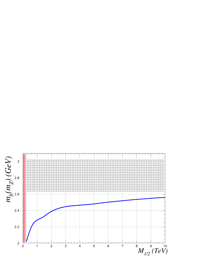
Figure 8: Bottom mass prediction from a minimal supersymmetric SU(5) exact fixed point with $\mu<0$ as a function of the gaugino mass. The shaded area represents the experimentally allowed region.

Typically, the preservation of naturalness, caused by quadratic divergences in the radiative corrections to the Higgs boson mass, is assumed to require superpartner masses below a few TeV. At present, supersymmetry is the only way we know to attack this problem. Although a rigorous definition of the concept is lacking, different sensitivity coefficients have been defined to measure the fine-tuning degree Ellis:1986yg ; Barbieri:1987fn ; anderson ; Chan:1997bi ; strumiafine ; deCarlos:yy . Some authors have found singularities resulting from numerical coincidences when plotting naturalness limits on scalar masses Barbieri:1987fn ; Ross:1992tz . This can be interpreted as allowing multi-TeV scalar masses Feng:1999mn .

Furthermore, all these criteria for fine-tuning have limitations. If there were some interrelation between different parameters caused by some fundamental dynamics that leads to the soft terms (such as the presence of a fixed point), it would show up in the form of strong correlations between parameters in the symmetry-breaking solutions; naïve fine-tuning criteria may then be inappropriate for analyzing the degree of fine-tuning Carena:1993bs . In our SU(5) fixed point scenario, all the soft parameters are proportional to the gaugino mass, while the Yukawa couplings are proportional to the unified gauge coupling, and $\tan\beta$ is computed from the tau lepton mass. At tree level, from the minimization equations, the $Z$ boson mass is reinterpreted as a function of the fundamental parameters,

$$m_{Z}^{2}=2\left(\alpha_{1/2}M_{1/2}^{2}-\mu^{2}\right),$$ (66)

where $\alpha_{1/2}$ is a positive constant. Using a common definition for the fine-tuning sensitivity coefficients Feng:1999mn , one finds that the fine-tuning of this model can be estimated by the expression

$$c_{\mu}=\left|\frac{\partial\ln m^{2}_{Z}}{\partial\ln\mu}\right|=\frac{4\mu^{2}}{m_{Z}^{2}}.$$ (67)

For the representative points in Table 6, $c_{\mu}$ thus goes from $3\times 10^{2}$ to $4\times 10^{4}$. In light of the successful predictions of this scenario, we may want to reconsider the use of fine-tuning constraints.

The large value of $c_{\mu}$ suggests that this scenario is fine-tuned so as to reproduce the experimental measurements. Furthermore, prospects for discovering multi-TeV squarks at the LHC have been considered colheavsca . From the sample spectra computed for the representative points in Table 6 we see that if the $SU(5)$ fixed point scenario is correct, it will probably not be possible to discover supersymmetric particles in the next generation of particle colliders if the gaugino mass is heavier than 1 TeV.

VI.4 Numerical results: threshold corrections

In Tables 7, 8, and 9 we include respectively, the dominant supersymmetric threshold corrections to top and bottom quarks and to the tau lepton, for the five representative points in Table 6. We observe that the logarithmic part of the gluino diagram is the dominant contribution to the supersymmetric thresholds for the top mass. This contribution is proportional to $\ln\left(m_{\widetilde{g}}/m_{t}\right)$, and we find numerically that it varies from $4\%$ (for small $M_{1/2}$) to $10\%$ (for very large values of $M_{1/2}$). Furthermore, we obtain that the prediction for the top mass is only weakly dependent on the gaugino unified mass. This is possible because when we increase the value of the gaugino unified mass, the supersymmetric thresholds to gauge couplings also increase, and as a consequence, we must decrease the unified gauge coupling to fit the experimental value of $\alpha_{s}^{\overline{\rm MS}}(m_{Z})$. When we decrease the unified gauge coupling at the fixed point, the top Yukawa coupling decreases (see Table 6), and as a consequence the tree-level component of the top quark gets smaller. The decrease in the tree-level component is partially counterbalanced with the increase in the threshold contribution, and the final prediction for the top pole mass is quite stable.

We now turn to the bottom mass thresholds. The supersymmetric radiative corrections to $m_{b}$ for the same representative points of our scans are shown for $\mu<0$ in Table 8. We see that the dominant correction comes from the finite piece of the gluino diagram and is negative for $\mu<0$, ranging from $-47\%$ (for small $M_{1/2}$) to $-32\%$ (for large $M_{1/2}$). This negative contribution is partially compensated by positive corrections caused by the logaritmic part of the gluino diagram and the chargino-stop loops. The chargino-stop contribution, Eq. (63), is almost independent of $M_{1/2}$ and represents around $14-16$%, while the gluino contribution increases with the gaugino mass, from $+5\%$ (for small $M_{1/2}$) to $+10\%$ (for very large values of $M_{1/2}$). We observe numerically that when we increase the gaugino mass, not only do the gaugino unified coupling and $\tan\beta$ decrease, but the ratio $\mu/m_{\widetilde{g}}$ also decreases. Therefore, from Eq. (62) we can easily understand why the finite part clearly decreases.

With regard to $\tan\beta$, we observe that it decreases when the gaugino mass increases. For $\mu<0$ we obtain $\tan\beta=51.65$ for $M_{1/2}=500$ GeV, and $\tan\beta=50.74$ for very large gaugino mass, $M_{1/2}=10$ TeV. As explained previously, $\tan\beta$ is determined using the tau mass. The threshold corrections to the tau mass are inversely correlated with the sign of $\mu$ and are around $8\%$, as can be seen in Table 9. These thresholds are crucial because the determination of $\tan\beta$ affects the bottom mass significantly. The inclusion of the tau thresholds represents a correction to the bottom mass of about $\pm~{}(6-7)\%$.

VI.5 Theoretical uncertainties

We will enumerate here the possible theoretical uncertainties in our predictions. In Tables 4 and 5, we gave our theoretical predictions including some errors. Let us clarify that those errors were due to the uncertainties in the experimental measurements of $\alpha_{s}(m_{Z})$ and $\alpha_{e}(m_{Z})$, which were used as contraints in our scans. Our numerical results must also contain some theoretical uncertainties, which we have not yet mentioned. These uncertainties would be related to the implementation of the radiative corrections in the low-energy MSSM and to the formulation of the GUT-scale initial conditions. With regard to the low-energy MSSM uncertainties, we note the following

• We have implemented the complete one-loop supersymmetric thresholds to fermion masses Pierce:1996zz . We have seen that the supersymmetric corrections to the bottom quark mass can be very important. One can wonder if the two-loop supersymmetric corrections to the bottom mass would be crucial for a more precise prediction of the bottom mass in this scenario. For instance, an additional $3\%$ uncertainty would translate into a $\pm 0.1$ GeV theoretical uncertainty.

• We have seen above that the leading logarithmic supersymmetric threshold corrections to the gauge couplings implemented in our analysis loggaug (mainly the strong gauge coupling threshold) can be very important, ranging from $+20\%$ to $+30\%$ for large gaugino masses. It is reasonable to think that the one-loop finite correction finitegaug and perhaps the two-loop SUSY thresholds may also be important for a more precise prediction of $s^{2}_{W}(m_{Z})$ and $m_{b}(m_{Z})$.

• The finite supersymmetric threshold corrections to the bottom mass are proportional to the $\mu$-term. In our analysis, the $\mu$-term is computed from the minimization equations at $m_{Z}$, including one loop sfermion corrections implemented using the effective potential as we explained in Sect. V. We have not included the remaining one-loop and two-loop corrections Martin:2002iu to the minimization equations. A small percentage of difference in the computation of the $\mu$-term could significantly affect the bottom mass prediction.

With regard to the GUT scale initial conditions, we note the following

• First, we assumed perfect gauge coupling unification. It is well-known that the GUT-scale threshold corrections to gauge coupling unification can be significant Wright:1994qb ; gutthres ; Antoniadis:1982vr . These effects would be interesting to include.

• We assumed the minimal supersymmetric SU(5) model. It is probable that we must add extra particle content to solve the problems that afflict the minimal SU(5) model Masina:2001pp . Additional matter content in the unified model would modify the fixed point predictions. We will estimate these effects in Sect. IX.

• Finally, we assumed that the boundary conditions for the MSSM at the unification scale satisfy the exact SU(5) fixed point predictions. It would be interesting to analyze how the low-energy predictions are affected by a small perturbation of the fixed point boundary conditions.

The successful predictions of our unified fixed point motivate a more precise study. The above uncertainties can be seen as a list of possible improvements if we want to go further in the analysis of this scenario.

parameters	$\Delta_{\widetilde{g}-Log}^{t}$	$\Delta^{t}_{\widetilde{g}-fin}$	$\Delta_{R}^{t}$	$\Delta^{t}_{\rm SUSY}$	$\Delta_{\rm QCD}^{t}$	$h_{t}(m_{t})v(m_{t})s_{\beta}$ (GeV)	$m_{t}$ (GeV)
point 1	$4.98\%$	$0.98\%$	$-1.47\%$	$4.49\%$	$5.98\%$	158.67	175.72
point 2	$6.68\%$	$0.93\%$	$-0.77\%$	$6.84\%$	$5.55\%$	154.94	174.73
point 3	$8.33\%$	$0.87\%$	$-0.05\%$	$9.15\%$	$5.15\%$	151.23	173.58
point 4	$8.87\%$	$0.86\%$	$0.12\%$	$9.85\%$	$5.04\%$	150.23	173.38
point 5	$9.31\%$	$0.84\%$	$0.10\%$	$10.25\%$	$4.94\%$	149.23	172.67

Table 7: One loop SUSY thresholds to the top quark mass evaluated at $m_{t}$ for the five points of Table 6. The last column, $m_{t}$, is the theoretical prediction for the pole mass after adding the SUSY thresholds, $\Delta^{t}_{\rm SUSY}$, and the gluon correction, $\Delta_{\rm QCD}^{t}$, to the tree-level part, $h_{t}(m_{t})v(m_{t})s_{\beta}$, included in the next-to-last column. $\Delta_{\widetilde{g}-Log}^{t}$ is the dominant contribution defined in Eq. (54), while $\Delta_{R}^{t}$ includes the rest of the one-loop SUSY corrections.

parameters	$\Delta_{\widetilde{g}-Log}^{b}$	$\Delta^{b}_{\widetilde{g}-Fin}$	$\Delta^{b}_{\widetilde{\chi}^{\pm}}$	$\Delta_{R}^{b}$	$\Delta^{b}_{\rm SUSY}$	$h_{b}(m_{Z})v(m_{Z})c_{\beta}$ (GeV)	$m_{b}^{\overline{\rm MS}}(m_{Z}^{>})$ (Gev)
point 1	$5.31\%$	$-46.79\%$	$15.80\%$	$4.16\%$	$-21.52\%$	$2.74$	$2.16$
point 2	$7.05\%$	$-40.91\%$	$15.10\%$	$5.40\%$	$-13.36\%$	2.68	$2.33$
point 3	$8.73\%$	$-35.41\%$	$14.19\%$	$6.97\%$	$-5.52\%$	2.62	$2.48$
point 4	$9.17\%$	$-33.98\%$	$13.87\%$	$7.37\%$	$-3.57\%$	2.61	$2.52$
point 5	$9.62\%$	$-32.52\%$	$13.55\%$	$7.80\%$	$-1.55\%$	2.60	$2.56$

Table 8: One-loop SUSY thresholds to the bottom quark mass evaluated at $M_{Z}$ for the five points of Table 6. The last column, $m_{b}^{\overline{\rm MS}}(m_{Z})$, is the theoretical prediction for the running mass at $m_{Z}$ after adding the SUSY thresholds, $\Delta^{b}_{\rm SUSY}$, to the tree-level part, $h_{b}(m_{Z})v(m_{Z})c_{\beta}$. $\Delta_{\widetilde{g}-Log}^{b}$, $\Delta^{b}_{\widetilde{g}-Fin}$ and $\Delta^{b}_{\widetilde{\chi}^{\pm}}$ are the dominant contributions defined in Eqs. (58), (60) and (63) respectively, while $\Delta_{R}^{b}$ includes the remaining one-loop SUSY corrections.

parameters	$\Delta_{\widetilde{\nu}_{\tau}-\widetilde{\chi}^{\pm}}^{\tau}$	$\Delta_{\widetilde{\tau}-\widetilde{\chi}^{0}}^{\tau}$	$\Delta_{R}^{\tau}$	$\Delta_{\rm SUSY}^{\tau}$	$h_{\tau}(m_{Z})v(m_{Z})c_{\beta}$  (GeV)	$m_{\tau}^{\overline{\rm MS}}(m_{Z}^{>})$ (GeV)	$t_{\beta}$
point 1	$6.26\%$	$2.02\%$	$0.06\%$	$8.34\%$	$1.6136$	1.7482	51.65
point 2	$5.74\%$	$2.07\%$	$0.30\%$	$8.11\%$	1.6169	1.7482	51.31
point 3	$5.35\%$	$2.23\%$	$0.59\%$	$8.17\%$	1.6162	1.7482	51.05
point 4	$5.15\%$	$2.24\%$	$0.66\%$	$8.05\%$	1.6178	1.7482	50.91
point 5	$4.94\%$	$2.21\%$	$0.73\%$	$7.88\%$	1.6204	1.7482	50.74

Table 9: One-loop supersymmetric radiative contributions to the tau lepton mass evaluated at $m_{Z}$ for the five representative points of Table 6. The last column, $m_{\tau}(m_{Z})$, is the theoretical prediction for the SM running mass at $m_{Z}$ after adding the SUSY thresholds, $\Delta_{\rm SUSY}^{\tau}$, to the tree level part, $h_{\tau}(m_{Z})v(m_{Z})c_{\beta}$. $\Delta_{\widetilde{\nu}_{\tau}-\widetilde{\chi}}^{\tau}$ is the dominant contribution defined in Eq. (65), while $\Delta_{R}^{\tau}$ includes the remaining one-loop SUSY corrections.

VII Fixed point predictions in non minimal SU(5) models

To solve the problems afflicting the minimal supersymmetric SU(5) model, extended non minimal models have been examined. For instance, it is known that one can fit the first and second generation standard model fermion masses and mixing angles, in the context of grand unified models, by adding extra matter to generate Yukawa textures at the GUT scale. Many of these extensions contain extra particle content, suggesting modifications to the minimal SU(5) fixed point predictions. Nonetheless, even though the evolution towards the Yukawa unified fixed point may occur more rapidly as a result of increased particle content, the fixed point for the soft parameters would become unstable if the added particle content were too large. For extensions of the minimal model, Eq. (4) applies with the modification $b=-3+S$, where $S$ is the sum of Dynkin indices of the additional fields dynkin . We are lacking a complete non minimal model for the soft sector and therefore do not know exactly the upper bound on $S$ imposed by soft stability. A naïve estimation, however, could be made based on Eq. (30).

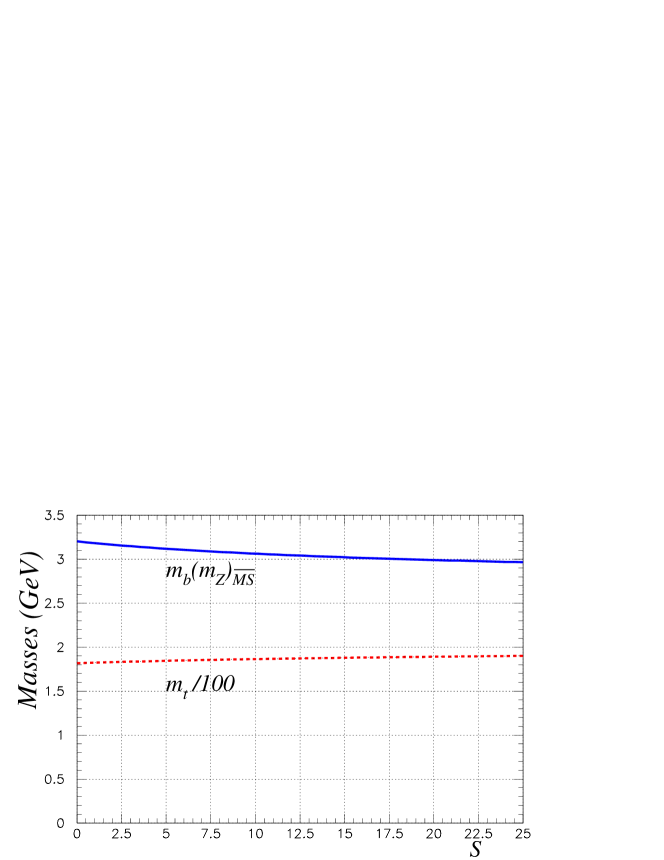
Figure 9: Top and bottom mass predictions, with no supersymmetric thresholds, from a non minimal supersymmetric SU(5) exact fixed point, with $\mu<0$, as a function of the Dynkin index. The value $S=0$ corresponds to minimal supersymmetric SU(5).

The fixed point solution for the Yukawa couplings in general non minimal models with extra particle content is given by

$$\frac{\lambda_{t}^{2}}{g^{2}}=\frac{2533}{2605}+\frac{145}{2605}~{}S,\qquad\frac{\lambda_{b}^{2}}{g^{2}}=\frac{1491}{2605}+\frac{145}{2605}~{}S,\qquad\frac{\lambda^{2}_{H}}{g^{2}}=\frac{560}{521}+\frac{30}{521}~{}S.$$ (68)

In principle $S>0$, so that $\lambda_{H}>1.036~{}g$, which is a good prediction since we overcome more easily the constraints on proton decay. Although we cannot make precise predictions for bottom and top masses, we can estimate, without a complete model of the soft sector of the non minimal model, how the extra particle content affects the mass predictions without including supersymmetric thresholds. Following the procedure used in Sec. II, we study the prediction for the top and bottom mass as a function of $S$. We show our results in Fig. 9. For $S=0$, we recover the minimal SU(5) predictions. The bottom mass prediction decreases from $3.2$ GeV for $S=0$ to $2.95$ GeV for $S=25$, while the top mass increases from $181$ GeV to $190$ GeV. Surprisingly, the effect of the extra matter is not so important as we expected at first sight from Eq. (68). We see that for $S=0$ the fixed point predicts $h_{t}=0.9860~{}g$, while for $S=25$ it predicts $h_{t}=1.5375~{}g$, representing a $56\%$ increase in the GUT scale inital condition. On the other hand, the top mass prediction increases only by $5\%$ while the bottom mass decreases by $8\%$. This effect is combined with a change in $\tan\beta$ when we increase the particle content. The reason is that when the tau Yukawa coupling grows, $\tan\beta$, which we compute using the tau mass, also increases. The bottom mass is especially affected, compensating for the increase in the bottom Yukawa coupling. Even though these conclusions are interesting, they must be considered preliminary, since non minimal models imply additional couplings, which affect the RGEs and can modify these predictions. Furthermore, we cannot include supersymmetric thresholds without a complete non minimal model for the soft sector.

VIII Yukawa unification and the large $\tan\beta$ fixed point in the MSSM

It seems, from our numerical results, that the SU(5) fixed point predictions, mainly the top quark mass, are more stable than one might have expected. The stability of these results could indicate the presence of fixed point behavior in the running of the MSSM Yukawa couplings from the GUT to the $m_{Z}$ scale. In the MSSM, there is a fixed point viable at large $\tan\beta$. The MSSM large $\tan\beta$ fixed point predicts that $h_{t}^{2}=h_{b}^{2}=g_{3}^{2}/3$ and $h_{\tau}=0$ in the infrared. The relevance of this fixed point in the context of top–bottom–tau unified models was pointed out in Ref. Schrempp:1994xn . The large $\tan\beta$ fixed point in the MSSM must not be confused with the low $\tan\beta$ fixed point. Even though the low $\tan\beta$ fixed point has been much more studied in the literature lowQFP , it is not relevant in the context of top-bottom-tau Yukawa unified models as it predicts that the bottom and tau Yukawa couplings are zero, while top-bottom unified models require that the top and bottom Yukawa couplings are of the same order at low energies. On the other hand, we think that even though the large $\tan\beta$ fixed point of the MSSM can be relevant in the SU(5) fixed point scenario, it is not predictive enough by itself to explain the measured third generation fermion masses, since it predicts that the tau Yukawa coupling is zero.

IX Summary and comments

In this paper we have outlined a precise analysis of the low-energy implications of a supersymmetric SU(5) fixed point. It is well known that supersymmetric grand unified theories predict correctly the weak mixing angle. This unified fixed point in addition predicts successfully the top quark mass without adjustments to any model parameter. This is, to my knowledge, the most successful prediction of the top mass in the literature based on first principles and implies that $175$ GeV is a number encoded in the symmetries of the supersymmetric SU(5) model. Other interesting predictions of the unified fixed point studied in this paper are

• the bottom mass, which is in general sensitive to the sign of $\mu$ and to the gaugino unified mass, approaches its experimental value for $\mu<0$ and very large values of the gaugino mass;

• the weak mixing angle is correctly predicted for low values of the gaugino unified mass, as is characteristic of other supersymmetric unified models, and can be successfully predicted for large values of the gaugino unified mass.

If the successful prediction of the weak mixing angle and the bottom mass (for very large gaugino unified mass) is more than a coincidence, it could be a hint that the mass scale of all supersymmetric particles lies well above 1 TeV. Furthermore, a very heavy SUSY spectrum would make other indirect supersymmetric signals unobservable in current experiments. The results found in this work may be regarded as evidence for supersymmetry with grand unification, especially as grand unification provides a simple and elegant explanation of the standard model gauge structure and representation content.

References

- (1) D. E. Groom et al. [Particle Data Group], Eur. Phys. J. C 15 (2000) 1.
- (2) H. Georgi and S. L. Glashow, Phys. Rev. Lett. 32 (1974) 438.
- (3) Supersymmetric extensions of the standard model provide a natural solution to the gauge hierarchy problem hierarchy and predict correctly the weak mixing angle, i.e. they incorporate the unification of gauge couplings.
- (4) M. J. Veltman, Acta Phys. Polon. B 12, 437 (1981); R. K. Kaul, Phys. Lett. B 109, 19 (1982).
- (5) M. B. Einhorn and D. R. Jones, Nucl. Phys. B 196, 475 (1982). J. R. Ellis, D. V. Nanopoulos and S. Rudaz, Nucl. Phys. B 202, 43 (1982); B. Ananthanarayan, G. Lazarides and Q. Shafi, Phys. Rev. D 44, 1613 (1991); H. Arason, D. J. Castano, B. Keszthelyi, S. Mikaelian, E. J. Piard, P. Ramond and B. D. Wright, Phys. Rev. D 46, 3945 (1992); V. D. Barger, M. S. Berger and P. Ohmann, Phys. Rev. D 47, 1093 (1993); P. Langacker and N. Polonsky, Phys. Rev. D 49, 1454 (1994); M. Carena, M. Olechowski, S. Pokorski and C. E. Wagner, Nucl. Phys. B 426, 269 (1994); H. Baer, M. A. Diaz, J. Ferrandis and X. Tata, Phys. Rev. D 61, 111701 (2000); H. Baer and J. Ferrandis, Phys. Rev. Lett. 87, 211803 (2001); T. Blazek, R. Dermisek and S. Raby, Phys. Rev. Lett. 88, 111804 (2002); T. Blazek, R. Dermisek and S. Raby, Phys. Rev. D 65, 115004 (2002)
- (6) The more complicated problem of the first- and second-generation fermion masses and mixing angles has also been addressed. Several Yukawa textures, in the context of different unified groups, have been studied in the literature. In these extended versions of the theory the high energy couplings must also be adjusted simultaneously to fit the low-energy data. In doing so one can ascertain the dominant operator contributions at the unification scale. See for instance: S. Raby, “Introduction to theories of fermion masses”, Published in 1994 Summer school in high energy physics and cosmology, World Scientific, 1995, [arXiv:hep-ph/9501349] S. Raby, “Testing theories of fermion masses”, Talk at SUSY2001, Dubna, Russia, 11-17 Jun 2001. [arXiv:hep-ph/0110203],and references therein.
- (7) B. Pendleton and G. G. Ross, Phys. Lett. B 98, 291 (1981)
- (8) J. Bagger, S. Dimopoulos and E. Masso, Phys. Rev. Lett. 55, 1450 (1985); J. Bagger, S. Dimopoulos and E. Masso, Phys. Rev. Lett. 55, 920 (1985); J. Bagger, S. Dimopoulos and E. Masso, Phys. Lett. B 156, 357 (1985); J. Bagger, S. Dimopoulos and E. Masso, Nucl. Phys. B 253, 397 (1985).
- (9) M. Lanzagorta and G. G. Ross, Phys. Lett. B 349, 319 (1995)
- (10) I. Masina, Int. J. Mod. Phys. A 16, 5101 (2001), see chapter (3) and references therein.
- (11) E. Witten, Nucl. Phys. B 188, 513 (1981).
- (12) N. Sakai, Z. Phys. C 11, 153 (1981).
- (13) S. Dimopoulos and H. Georgi, Nucl. Phys. B 193, 150 (1981).
- (14) N. Polonsky and A. Pomarol, Phys. Rev. D 51, 6532 (1995); N. Polonsky and A. Pomarol, Phys. Rev. Lett. 73, 2292 (1994)
- (15) R. Barbieri, L. J. Hall and A. Strumia, Nucl. Phys. B 445, 219 (1995); P. Ciafaloni, A. Romanino and A. Strumia, Nucl. Phys. B 458, 3 (1996)
- (16) J. Bagger, J. L. Feng and N. Polonsky, Nucl. Phys. B 563, 3 (1999)
- (17) B. C. Allanach and S. F. King, Phys. Lett. B 407, 124 (1997)
- (18) P. Langacker, Phys. Rept. 72 (1981) 185; S. Dimopoulos, S. Raby and F. Wilczek, Phys. Lett. B 112 (1982) 133; R. Arnowitt and P. Nath, Phys. Rev. Lett. 69, 725 (1992); P. Nath and R. Arnowitt, Phys. Lett. B 287, 89 (1992); J. Hisano, H. Murayama and T. Yanagida, Nucl. Phys. B 402, 46 (1993); R. Dermisek, A. Mafi and S. Raby, Phys. Rev. D 63, 035001 (2001); H. Murayama and A. Pierce, Phys. Rev. D 65, 055009 (2002); B. Bajc, P. F. Perez and G. Senjanovic, [arXiv:hep-ph/0204311]
- (19) H. Arason, D. J. Castano, B. Keszthelyi, S. Mikaelian, E. J. Piard, P. Ramond and B. D. Wright, Phys. Rev. D 46, 3945 (1992);
- (20) B. D. Wright, “Yukawa coupling thresholds: Application to the MSSM and the minimal supersymmetric SU(5) GUT,” [arXiv:hep-ph/9404217]
- (21) H. Baer, J. Ferrandis, K. Melnikov and X. Tata, Phys. Rev. D 66, 074007 (2002)
- (22) I. Antoniadis, C. Kounnas and K. Tamvakis, Phys. Lett. B 119, 377 (1982).
- (23) R. Tarrach, Nucl. Phys. B 183, 384 (1981).
- (24) L. V. Avdeev and M. Y. Kalmykov, Nucl. Phys. B 502, 419 (1997)
- (25) K. Melnikov and T. v. Ritbergen, Phys. Lett. B 482, 99 (2000) K. G. Chetyrkin and M. Steinhauser, Nucl. Phys. B 573, 617 (2000) K. G. Chetyrkin, J. H. Kuhn and M. Steinhauser, Comput. Phys. Commun. 133, 43 (2000)
- (26) I. Jack, D. R. Jones, S. P. Martin, M. T. Vaughn and Y. Yamada, Phys. Rev. D 50, 5481 (1994); I. Jack and D. R. Jones, Phys. Lett. B 333, 372 (1994); Y. Yamada, Phys. Rev. D 50, 3537 (1994); S. P. Martin and M. T. Vaughn, Phys. Rev. D 50, 2282 (1994); V. D. Barger, M. S. Berger and P. Ohmann, Phys. Rev. D 47, 1093 (1993)
- (27) We use two-loop RGEs for the MSSM couplings as implemented in ISASUGRA. For additional information you can visit ISAJET homepage at http://www.bnl.gov/isajet. ISAJET manual is available in the arXiv.org eprint archive, see H. Baer, F. E. Paige, S. D. Protopopescu and X. Tata, “ISAJET 7.48: A Monte Carlo event generator for p p, anti-p p, and e+ e- reactions,” [arXiv:hep-ph/0001086]
- (28) D. M. Pierce, J. A. Bagger, K. T. Matchev and R. j. Zhang, Nucl. Phys. B 491, 3 (1997)
- (29) K. Inoue, A. Kakuto, H. Komatsu and S. Takeshita, Prog. Theor. Phys. 67, 1889 (1982); L. E. Ibanez and C. Lopez, Nucl. Phys. B 233, 511 (1984).
- (30) R. Hempfling, Z. Phys. C 63, 309 (1994); L. J. Hall, R. Rattazzi and U. Sarid, Phys. Rev. D 50, 7048 (1994); M. Carena, M. Olechowski, S. Pokorski and C. E. Wagner, Nucl. Phys. B 426, 269 (1994); T. Blazek, S. Raby and S. Pokorski, Phys. Rev. D 52, 4151 (1995)
- (31) L. Girardello and M. T. Grisaru, Nucl. Phys. B 194, 65 (1982).
- (32) L. F. Li, Phys. Rev. D 9, 1723 (1974); A. J. Buras, J. R. Ellis, M. K. Gaillard and D. V. Nanopoulos, Nucl. Phys. B 135, 66 (1978); M. Magg and Q. Shafi, Z. Phys. C 4, 63 (1980); F. Buccella, H. Ruegg and C. A. Savoy, Nucl. Phys. B 169, 68 (1980).
- (33) N. V. Dragon, Phys. Lett. B 113, 288 (1982); N. Dragon, Z. Phys. C 15, 169 (1982); F. Buccella, J. P. Derendinger, S. Ferrara and C. A. Savoy, Phys. Lett. B 115, 375 (1982).
- (34) I. Jack and D. R. Jones, Phys. Lett. B 443, 177 (1998)
- (35) It has also been pointed out by I. Jack and D.R.T. Jones that, under certain conditions for the dimensionless couplings, there are RG-invariant universal forms for the soft paramaters, and that these may also constitute an IR fixed point that may be approached closely at the unification scale. I. Jack, D. R. Jones and K. L. Roberts, Nucl. Phys. B 455, 83 (1995); P. M. Ferreira, I. Jack and D. R. Jones, Phys. Lett. B 357, 359 (1995)
- (36) M. Lanzagorta and G. G. Ross, Phys. Lett. B 364, 163 (1995)
- (37) G. Amelino-Camelia, “Simple GUTs”, Talk given at 9th International Seminar on High-energy Physics: Quarks 96, Yaroslavl, Russia,5-11 May 1996, [arXiv:hep-ph/9610298]
- (38) There have been previous attempts to understand the SU(5) spontaneous symmetry-breaking pattern as a possible result of the renormalization group flow. B. C. Allanach, G. Amelino-Camelia, O. Philipsen, O. Pisanti and L. Rosa, Nucl. Phys. B 537, 32 (1999); B. C. Allanach, G. Amelino-Camelia and O. Philipsen, Phys. Lett. B 393, 349 (1997);
- (39) J. E. Kim and H. P. Nilles, Phys. Lett. B 138, 150 (1984).
- (40) es R. Arnowitt and P. Nath, Phys. Rev. D 46, 3981 (1992)
- (41) Y. Okada, M. Yamaguchi and T. Yanagida, Prog. Theor. Phys. 85, 1 (1991) ; H. E. Haber and R. Hempfling, Phys. Rev. Lett. 66, 1815 (1991) ; J. R. Ellis, G. Ridolfi and F. Zwirner, Phys. Lett. B 257, 83 (1991) ; J. R. Ellis, G. Ridolfi and F. Zwirner, Phys. Lett. B 262, 477 (1991) ; A. Brignole, J. R. Ellis, G. Ridolfi and F. Zwirner, Phys. Lett. B 271, 123 (1991)
- (42) P. Langacker and N. Polonsky, Phys. Rev. D 47, 4028 (1993); M. Carena, S. Pokorski and C. E. Wagner, Nucl. Phys. B 406, 59 (1993); P. Langacker and N. Polonsky, Phys. Rev. D 52, 3081 (1995)
- (43) S. Dimopoulos, S. Raby and F. Wilczek, Phys. Rev. D 24, 1681 (1981); U. Amaldi, W. de Boer and H. Furstenau, Phys. Lett. B 260, 447 (1991); J. R. Ellis, S. Kelley and D. V. Nanopoulos, Phys. Lett. B 260, 131 (1991); P. Langacker and M. X. Luo, Phys. Rev. D 44, 817 (1991)
- (44) J. R. Ellis, K. Enqvist, D. V. Nanopoulos and F. Zwirner, Mod. Phys. Lett. A 1, 57 (1986).
- (45) R. Barbieri and G. F. Giudice, Nucl. Phys. B 306, 63 (1988)
- (46) G. W. Anderson and D. J. Castano, Phys. Lett. B 347, 300 (1995); G. W. Anderson and D. J. Castano, Phys. Rev. D 52, 1693 (1995); G. W. Anderson and D. J. Castano, Phys. Rev. D 53, 2403 (1996)
- (47) K. L. Chan, U. Chattopadhyay and P. Nath, Phys. Rev. D 58, 096004 (1998)
- (48) R. Barbieri and A. Strumia, Phys. Lett. B 433, 63 (1998) L. Giusti, A. Romanino and A. Strumia, Nucl. Phys. B 550, 3 (1999); A. Strumia, “Naturalness of supersymmetric models,” [arXiv:hep-ph/9904247]; A. Romanino and A. Strumia, Phys. Lett. B 487, 165 (2000) R. Barbieri and A. Strumia, “The ’LEP paradox’,” [arXiv:hep-ph/0007265]; R. Barbieri and A. Strumia, Phys. Lett. B 490, 247 (2000)
- (49) B. de Carlos and J. A. Casas, Phys. Lett. B 309, 320 (1993)
- (50) G. G. Ross and R. G. Roberts, Nucl. Phys. B 377, 571 (1992); P. H. Chankowski, J. R. Ellis, M. Olechowski and S. Pokorski, Nucl. Phys. B 544, 39 (1999); P. H. Chankowski, J. R. Ellis and S. Pokorski, Phys. Lett. B 423, 327 (1998); G. L. Kane and S. F. King, Phys. Lett. B 451, 113 (1999)
- (51) J. L. Feng, K. T. Matchev and T. Moroi, Phys. Rev. Lett. 84, 2322 (2000); J. L. Feng and K. T. Matchev, Phys. Rev. D 63, 095003 (2001); S. Dimopoulos and G. F. Giudice, Phys. Lett. B 357, 573 (1995)
- (52) M. Carena, M. Olechowski, S. Pokorski and C. E. Wagner, Nucl. Phys. B 419, 213 (1994);
- (53) B. C. Allanach, J. P. Hetherington, M. A. Parker and B. R. Webber, JHEP 0008, 017 (2000); U. Chattopadhyay, A. Datta, A. Datta, A. Datta and D. P. Roy, Phys. Lett. B 493, 127 (2000); J. L. Feng, K. T. Matchev and T. Moroi, Phys. Rev. D 61, 075005 (2000)
- (54) P. H. Chankowski, Z. Pluciennik and S. Pokorski, Nucl. Phys. B 439, 23 (1995); R. Barbieri, P. Ciafaloni and A. Strumia, Nucl. Phys. B 442, 461 (1995)
- (55) S. P. Martin, Phys. Rev. D 66, 096001 (2002)
- (56) J. Bagger, K. T. Matchev and D. Pierce, Phys. Lett. B 348, 443 (1995); Y. Yamada, Z. Phys. C 60, 83 (1993). J. Hisano, H. Murayama and T. Yanagida, Phys. Rev. Lett. 69, 1014 (1992); K. Hagiwara and Y. Yamada, Phys. Rev. Lett. 70, 709 (1993); M. B. Einhorn and D. R. Jones, Nucl. Phys. B 196, 475 (1982);
- (57) B. Schrempp, Phys. Lett. B 344, 193 (1995)
- (58) V. D. Barger, M. S. Berger, P. Ohmann and R. J. Phillips, Phys. Lett. B 314, 351 (1993); W. A. Bardeen, M. Carena, S. Pokorski and C. E. Wagner, Phys. Lett. B 320, 110 (1994); M. Carena and C. E. Wagner, arXiv:[hep-ph/9407208]; M. Carena and C. E. Wagner, Nucl. Phys. B 452, 45 (1995) B. Brahmachari, Mod. Phys. Lett. A 12, 1969 (1997); S. A. Abel and B. Allanach, Phys. Lett. B 415, 371 (1997); J. A. Casas, J. R. Espinosa and H. E. Haber, Nucl. Phys. B 526, 3 (1998) G. K. Yeghian, M. Jurcisin and D. I. Kazakov, Mod. Phys. Lett. A 14, 601 (1999)
- (59) S. P. Martin, Phys. Rev. D 65, 035003 (2002)
- (60) For convenience a few typical SU(5) representations and their Dynkin indices are listed here: , , , , , and .