From DIS to proton-nucleus collisions
in the Color Glass Condensate model

Abstract

We show that particle production in proton-nucleus (pA) collisions in the Color Glass Condensate model can be related to Deep Inelastic Scattering of leptons on protons/nuclei (DIS). The common building block is the quark antiquark (or gluon-gluon) dipole cross section which is present in both DIS and pA processes. This correspondence in a sense generalizes the standard leading twist approach to pA collisions based on collinear factorization and perturbative QCD, and allows one to express the pA cross sections in terms of a universal quantity (dipole cross section) which, in principle, can be measured in DIS or other processes. Therefore, using the parameterization of dipole cross section at HERA, one can calculate particle production cross sections in proton-nucleus collisions at high energies. Alternatively, one could use proton-nucleus experiments to further constrain models of the dipole cross-section. We show that the McLerran-Venugopalan model predicts enhancement of cross sections at large $p_{\perp}$ (Cronin effect) and suppression of cross sections at low $p_{\perp}$. The cross over depends on rapidity and moves to higher $p_{\perp}$ as one goes to more forward rapidities.

1. Service de Physique Théorique
   Bât. 774, CEA/DSM/Saclay
   91191, Gif-sur-Yvette Cedex, France

2. Physics Department
   Brookhaven National Laboratory
   Upton, NY 11973, USA

SPhT-T02/167

1 Introduction

High gluon density effects at high energy (small $x$) have been the subject of intense theoretical and experimental investigation [1, 2, 3, 4, 5, 6, 7, 8, 9, 10, 11, 12, 13, 14, 15, 16, 17, 18, 19, 20]. At small $x$, the number of gluons per unit area and rapidity in the wave function of a high energy hadron or nucleus becomes large and the high energy hadron or nucleus can be described by a classical color field. Since most of the gluons in the wave function of a high energy hadron or nucleus are in a coherent state characterized by their typical momentum $Q_{s}$, a high energy hadron or nucleus is dubbed a Color Glass Condensate. An effective action and renormalization group approach has been developed which enables one to calculate cross sections in a high gluon density environment.

In [21, 22, 23, 24], for proton-nucleus collisions at high energies and in the forward rapidity region we proposed describing the proton by the QCD parton model and the nucleus by the Color Glass Condensate model. One can then relate particle production in proton-nucleus collisions to the scattering of a quark or gluon from the Color Glass Condensate [21, 22, 23, 24]. Here we show that one can relate particle production in proton-nucleus collisions to Deep Inelastic Scattering of electrons (or more precisely, virtual photons) on protons and nuclei. This is due to the fact that the description of the target as a Color Glass Condensate is universal and independent of the process considered.

While the relation between particle production in proton-nucleus collisions and DIS structure functions has been known for a while in the case of dilepton (virtual photon) production [25, 26] (and references therein), here we show that this relation is more general in our framework and holds for production of any particle (which has a known fragmentation function) in proton-nucleus collisions at high energy. This is crucial in view of the upcoming proton (deuteron)-nucleus experiments at RHIC. One would like to have predictions from QCD with as few model dependent assumptions about nuclear effects as possible.

In proton-proton collisions, standard calculations are based on collinear factorization theorems, proven at the leading twist level. The predictability of the theory is due to the fact that the building blocks (distribution or fragmentation functions) used in the cross section are universal (i.e. process independent) objects which can be measured in a given process and used to predict the outcome of other processes. It is well known that higher twist effects break collinear factorization and one has to resort to other methods. In proton-nucleus collisions, in order to take nuclear modifications such as shadowing and Cronin effect into account, one commonly modifies the parton distributions to include nuclear shadowing and introduces some model for Cronin effect. The parameters of the model are then constrained by fits to the existing data and used to make predictions for other processes or higher energies.

However, it is clear that this approach cannot be true in general since collinear factorization theorems break down due to higher twist (multiple scatterings) effects which become significant in scattering off nuclei. Therefore there is no guarantee that the parameters of such models are universal and process independent and these models have little predictive power. Here we show that one can generalize the standard leading twist expressions in such a way that all higher twist effects are included and the universality of the building blocks (dipole cross sections) of the theory is preserved and the predictive power of the theory is restored.

2 Reminder: DIS and the dipole cross-section

2.1 DIS amplitude

We first start by a brief reminder of how the dipole cross-section appears in Deep Inelastic Scattering. This calculation will in fact be useful in order to compare with the very similar problem of dilepton (i.e. virtual photon) production in pA collisions. The nucleus is treated using the Color Glass Condensate model, i.e. as a set of classical and randomly distributed color sources that generate a classical field. There are three relevant diagrams for the DIS amplitude in this model, which are represented in figure 1.

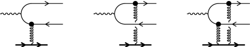
Figure 1: The relevant diagrams for $\gamma^{*}A\to q\bar{q}X$ in the Color Glass Condensate model. The black dots denote the eikonal interaction between the quark or antiquark with the classical color field.

In this figure, the black dot denotes the eikonal all-orders interaction between a quark or antiquark with the classical field of the nucleus. More precisely, for a quark or antiquark line in which the incoming momentum is $P$ and the outgoing momentum is $Q$, the (time-ordered) eikonal scattering amplitude reads

$$T_{\rm eik}(Q,P)=2\pi\delta(q^{-}-p^{-})\gamma^{-}{\rm sign}(p^{-})\int d{\boldsymbol{x}}_{\perp}e^{i({\boldsymbol{q}}_{\perp}-{\boldsymbol{p}}_{\perp})\cdot{\boldsymbol{x}}_{\perp}}\left(U^{{\rm sign}(p^{-})}({\boldsymbol{x}}_{\perp})\!-1\!\right)\;,$$ (1)

where we assume that the nucleus is moving close to the speed of light in the $+z$ direction. $U({\boldsymbol{x}}_{\perp})$ is a matrix living in the fundamental representation of $SU(N_{c})$, given by

$$U({\tenimbf x}_{\perp})\equiv{\rm T}\exp\bigg{\{}-ig^{2}\int^{+\infty}_{-\infty}dz^{-}{1\over{\nabla^{2}_{\perp}}}\rho_{a}(z^{-},{\tenimbf z}_{\perp})t^{a}\bigg{\}}\;,$$ (2)

with $t^{a}$ in the fundamental representation, and where $\rho_{a}(z^{-},{\tenimbf z}_{\perp})$ is the density of color sources in the nucleus. How to average over these sources is explained in [27, 23].

We first compute the $\gamma^{*}A\to q\bar{q}X$ amplitude, and bring it to a form that will be easy to compare with the photon production amplitude. A straightforward use of the CGC rules (see [27, 28, 23, 24] for details and examples) gives for this amplitude the following sum of three terms, each corresponding to a diagram in figure 1:

$$\!\!\!\!{\cal M}^{\mu}_{{}_{DIS}}({\boldsymbol{k}}|{\boldsymbol{q}},{\boldsymbol{p}})=-i\int d^{2}{\boldsymbol{x}}_{2\perp}e^{i({\boldsymbol{q}}_{\perp}+{\boldsymbol{p}}_{\perp}-{\boldsymbol{k}}_{\perp})\cdot{\boldsymbol{x}}_{2\perp}}\left(U^{\dagger}({\boldsymbol{x}}_{2\perp})-1\right)$$

$$\qquad\qquad\times\overline{u}({\boldsymbol{q}})\left[\frac{\gamma^{\mu}(\raise 0.6458pt\hbox{$/$}\kern-5.29999pt\hbox{$Q$}-\raise 0.6458pt\hbox{$/$}\kern-5.29999pt\hbox{$K$}+m)\gamma^{-}}{(Q-K)^{2}-m^{2}+i\epsilon}\right]v({\boldsymbol{p}})$$

$$+i\int d^{2}{\boldsymbol{x}}_{1\perp}e^{i({\boldsymbol{q}}_{\perp}+{\boldsymbol{p}}_{\perp}-{\boldsymbol{k}}_{\perp})\cdot{\boldsymbol{x}}_{1\perp}}\left(U({\boldsymbol{x}}_{1\perp})-1\right)$$

$$\qquad\qquad\times\overline{u}({\boldsymbol{q}})\left[\frac{\gamma^{-}(\raise 0.6458pt\hbox{$/$}\kern-5.29999pt\hbox{$K$}-\raise 0.6458pt\hbox{$/$}\kern-5.29999pt\hbox{$P$}+m)\gamma^{\mu}}{(P-K)^{2}-m^{2}+i\epsilon}\right]v({\boldsymbol{p}})$$

$$+i\int\frac{d^{2}{\boldsymbol{l}}_{\perp}}{(2\pi)^{2}}\int d^{2}{\boldsymbol{x}}_{1\perp}d^{2}{\boldsymbol{x}}_{2\perp}$$

$$\,\;\times e^{i{\boldsymbol{l}}_{\perp}\cdot{\boldsymbol{x}}_{1\perp}}e^{i({\boldsymbol{p}}_{\perp}+{\boldsymbol{q}}_{\perp}-{\boldsymbol{k}}_{\perp}-{\boldsymbol{l}}_{\perp})\cdot{\boldsymbol{x}}_{2\perp}}\left(U({\boldsymbol{x}}_{1\perp})-1\right)\left(U^{\dagger}({\boldsymbol{x}}_{2\perp})-1\right)$$

$$\;\,\times\overline{u}({\boldsymbol{q}})\!\left[\frac{\gamma^{-}(\raise 0.6458pt\hbox{$/$}\kern-5.29999pt\hbox{$Q$}-\raise 0.6458pt\hbox{$/$}\kern-5.29999pt\hbox{$L$}+m)\gamma^{\mu}(\raise 0.6458pt\hbox{$/$}\kern-5.29999pt\hbox{$Q$}-\raise 0.6458pt\hbox{$/$}\kern-5.29999pt\hbox{$K$}-\raise 0.6458pt\hbox{$/$}\kern-5.29999pt\hbox{$L$}+m)\gamma^{-}}{2p^{-}[({\boldsymbol{q}}_{\perp}\!-\!{\boldsymbol{l}}_{\perp})^{2}+m^{2}\!-\!2q^{-}k^{+}]+2q^{-}[({\boldsymbol{q}}_{\perp}\!-\!{\boldsymbol{k}}_{\perp}\!-\!{\boldsymbol{l}}_{\perp})^{2}+m^{2}]}\right]\!v({\boldsymbol{p}})\;.$$

(3)

In this equation $Q,P$ and $K$ are the momenta of the outgoing quark, outgoing antiquark and incoming photon respectively, ${\boldsymbol{x}}_{1\perp}$ and ${\boldsymbol{x}}_{2\perp}$ are the coordinates in impact parameter space of the quark and antiquark. In the third diagram, the momentum $L$ is the momentum transferred between the nucleus and the quark line. Its $-$ component is zero because the nucleus is moving at the speed of light in the $+z$ direction, and its $+$ component has already been integrated out by using the theorem of residues (we pick the pole in the upper half-plane, at $l^{+}=q^{+}-[({\boldsymbol{q}}_{\perp}-{\boldsymbol{l}}_{\perp})^{2}+m^{2}-i\epsilon]/2q^{-}$).

At this point, it is useful to note that since $P$ and $Q$ are on-shell, we have the following two identities:

$$\overline{u}({\boldsymbol{q}})=\frac{1}{2q^{-}}\overline{u}({\boldsymbol{q}})\gamma^{-}(m+\raise 0.6458pt\hbox{$/$}\kern-5.29999pt\hbox{$Q$})\;,$$

$$v({\boldsymbol{p}})=-\frac{1}{2p^{-}}(m-\raise 0.6458pt\hbox{$/$}\kern-5.29999pt\hbox{$P$})\gamma^{-}v({\boldsymbol{p}})\;.$$ (4)

Inserting them respectively in the first and second term of Eq. (3), and introducing also a dummy variable ${\boldsymbol{l}}_{\perp}$ via $\int d^{2}{\boldsymbol{x}}_{1\perp}d^{2}{{\boldsymbol{l}}_{\perp}}/(2\pi)^{2}\exp(i{\boldsymbol{l}}_{\perp}\cdot{\boldsymbol{x}}_{1\perp})$ or $\int d^{2}{\boldsymbol{x}}_{2\perp}d^{2}{{\boldsymbol{l}}_{\perp}}/(2\pi)^{2}\exp(i{\boldsymbol{l}}_{\perp}\cdot{\boldsymbol{x}}_{2\perp})$, we can combine three terms into one:

$${\cal M}^{\mu}_{{}_{DIS}}({\boldsymbol{k}}|{\boldsymbol{q}},{\boldsymbol{p}})=\frac{i}{2}\int\frac{d^{2}{\boldsymbol{l}}_{\perp}}{(2\pi)^{2}}\int d^{2}{\boldsymbol{x}}_{1\perp}d^{2}{\boldsymbol{x}}_{2\perp}$$

$$\qquad\;\times e^{i{\boldsymbol{l}}_{\perp}\cdot{\boldsymbol{x}}_{1\perp}}e^{i({\boldsymbol{p}}_{\perp}+{\boldsymbol{q}}_{\perp}-{\boldsymbol{k}}_{\perp}-{\boldsymbol{l}}_{\perp})\cdot{\boldsymbol{x}}_{2\perp}}\left(U({\boldsymbol{x}}_{1\perp})U^{\dagger}({\boldsymbol{x}}_{2\perp})-1\right)\;$$

$$\qquad\;\times\overline{u}({\boldsymbol{q}})\,\Gamma^{\mu}(k^{\pm},{\boldsymbol{k}}_{\perp}|q^{-},p^{-},{\boldsymbol{q}}_{\perp}-{\boldsymbol{l}}_{\perp})\,v({\boldsymbol{p}})\;,$$ (5)

where we denote

$$\Gamma^{\mu}(k^{\pm},{\boldsymbol{k}}_{\perp}|q^{-},p^{-},{\boldsymbol{q}}_{\perp}-{\boldsymbol{l}}_{\perp})\equiv$$

$$\qquad\equiv\frac{\gamma^{-}(\raise 0.6458pt\hbox{$/$}\kern-5.29999pt\hbox{$Q$}-\raise 0.6458pt\hbox{$/$}\kern-5.29999pt\hbox{$L$}+m)\gamma^{\mu}(\raise 0.6458pt\hbox{$/$}\kern-5.29999pt\hbox{$Q$}-\raise 0.6458pt\hbox{$/$}\kern-5.29999pt\hbox{$K$}-\raise 0.6458pt\hbox{$/$}\kern-5.29999pt\hbox{$L$}+m)\gamma^{-}}{p^{-}[({\boldsymbol{q}}_{\perp}\!-\!{\boldsymbol{l}}_{\perp})^{2}+m^{2}\!-\!2q^{-}k^{+}]+q^{-}[({\boldsymbol{q}}_{\perp}\!-\!{\boldsymbol{k}}_{\perp}\!-\!{\boldsymbol{l}}_{\perp})^{2}+m^{2}]}\;.$$ (6)

This is our final expression for the DIS amplitude off the target color field. Note that $\Gamma^{\mu}$ a priori depends on ${\boldsymbol{p}}_{\perp}$ and ${\boldsymbol{q}}_{\perp}$. However, in its list of arguments, we have anticipated the fact that the ${\boldsymbol{p}}_{\perp}$ and ${\boldsymbol{q}}_{\perp}$ that comes from the spinors drops out in physical quantities, because in the squared amplitude they always appear in combinations such as $\gamma^{-}u({\boldsymbol{q}})\overline{u}({\boldsymbol{q}})\gamma^{-}=2q^{-}\gamma^{-}$. In Eq. (5), $\Gamma^{\mu}$ is a quantity which describes how the virtual photon splits into a $q\bar{q}$ pair, which longitudinal momenta $q^{-},p^{-}$ and transverse momentum of the quark ${\boldsymbol{q}}_{\perp}-{\boldsymbol{l}}_{\perp}$, while the factor $U({\boldsymbol{x}}_{1\perp})U^{\dagger}({\boldsymbol{x}}_{2\perp})-1$ can be seen as the scattering amplitude of the dipole on color field of the nucleus.

2.2 DIS Cross-section

From Eq. (5), one can obtain the $\gamma^{*}A$ cross-section as

$$d\sigma_{{}_{DIS}}=\frac{d^{3}{\boldsymbol{q}}}{(2\pi)^{2}2q_{0}}\frac{d^{3}{\boldsymbol{p}}}{(2\pi)^{3}2p_{0}}\frac{1}{2k^{-}}2\pi\delta(k^{-}-p^{-}-q^{-})$$

$$\qquad\qquad\times\left<{\cal M}^{\mu}_{{}_{DIS}}({\boldsymbol{k}}|{\boldsymbol{q}},{\boldsymbol{p}}){\cal M}^{\nu*}_{{}_{DIS}}({\boldsymbol{k}}|{\boldsymbol{q}},{\boldsymbol{p}})\right>_{\rho}\epsilon_{\mu}(K)\epsilon_{\nu}^{*}(K)\;,$$ (7)

where $\left<\cdots\right>_{\rho}$ denotes the average over the color sources and where $\epsilon^{\mu}(K)$ is the polarization vector of the photon. At this point, in order to exploit the fact that $\Gamma^{\mu}$ depends only on ${\boldsymbol{m}}_{\perp}\equiv{\boldsymbol{q}}_{\perp}-{\boldsymbol{l}}_{\perp}$, we can use this quantity as the integration variable in ${\cal M}^{\mu}_{{}_{DIS}}$, and we can integrate out trivially the transverse momenta ${\boldsymbol{q}}_{\perp}$ and ${\boldsymbol{p}}_{\perp}$ of the quark and antiquark in the final state, in order to obtain:

$$\sigma_{{}_{DIS}}=\frac{1}{32\pi k_{-}^{2}}\int_{0}^{1}\frac{dz}{z(1-z)}\int d^{2}{\boldsymbol{r}}_{\perp}\int\frac{d^{2}{\boldsymbol{m}}_{\perp}}{(2\pi)^{2}}\frac{d^{2}{\boldsymbol{m}}^{\prime}_{\perp}}{(2\pi)^{2}}\,\epsilon_{\mu}(k)\epsilon_{\nu}^{*}(k)$$

$$\!\!\!\!\!\!\!\!\times e^{i({\boldsymbol{m}}_{\perp}-{\boldsymbol{m}}^{\prime}_{\perp})\cdot{\boldsymbol{r}}_{\perp}}\int d^{2}{\boldsymbol{X}}_{\perp}\;{\rm Tr}_{c}\left(1-{\rm Re}\left<U({\boldsymbol{X}}_{\perp}+\frac{{\boldsymbol{r}}_{\perp}}{2})U^{\dagger}({\boldsymbol{X}}_{\perp}-\frac{{\boldsymbol{r}}_{\perp}}{2})\right>_{\rho}\right)$$

$$\!\!\!\!\!\!\!\!\times{\rm Tr}_{d}\left((\raise 0.43057pt\hbox{$/$}\kern-6.30005pt\hbox{$q$}+m)\Gamma^{\mu}(k^{\pm},{\boldsymbol{k}}_{\perp}|q^{-},p^{-},{\boldsymbol{m}}_{\perp})(\raise 0.43057pt\hbox{$/$}\kern-6.30005pt\hbox{$p$}-m)\Gamma^{\nu\dagger}(k^{\pm},{\boldsymbol{k}}_{\perp}|q^{-},p^{-},{\boldsymbol{m}}^{\prime}_{\perp})\right)\;,$$ (8)

with $z$ the momentum fraction $z\equiv q^{-}/k^{-}$ ($p^{-}=(1-z)k^{-}$), where ${\rm Tr}_{c}$ denotes the color trace and ${\rm Tr}_{d}$ the Dirac trace, and where we have introduced the dipole size ${\boldsymbol{r}}_{\perp}\equiv{\boldsymbol{x}}_{1\perp}-{\boldsymbol{x}}_{2\perp}$ and barycenter ${\boldsymbol{X}}_{\perp}\equiv({\boldsymbol{x}}_{1\perp}+{\boldsymbol{x}}_{2\perp})/2$. If we introduce the dipole cross-section

$$\sigma_{\rm dipole}({\boldsymbol{r}}_{\perp})\equiv\frac{2}{N_{c}}\int d^{2}{\boldsymbol{X}}_{\perp}\;{\rm Tr}_{c}\left<1-U({\boldsymbol{X}}_{\perp}+\frac{{\boldsymbol{r}}_{\perp}}{2})U^{\dagger}({\boldsymbol{X}}_{\perp}-\frac{{\boldsymbol{r}}_{\perp}}{2})\right>_{\rho}$$ (9)

and the square of the photon wave function:

$$\left|\Psi(k^{\pm},{\boldsymbol{k}}_{\perp}|z,{\boldsymbol{r}}_{\perp})\right|^{2}\equiv\frac{N_{c}\,\epsilon_{\mu}(K)\epsilon_{\nu}^{*}(K)}{64\pi k_{-}^{2}z(1-z)}\int\frac{d^{2}{\boldsymbol{m}}_{\perp}}{(2\pi)^{2}}\frac{d^{2}{\boldsymbol{m}}^{\prime}_{\perp}}{(2\pi)^{2}}e^{i({\boldsymbol{m}}_{\perp}-{\boldsymbol{m}}^{\prime}_{\perp})\cdot{\boldsymbol{r}}_{\perp}}$$

$$\quad\times{\rm Tr}_{d}\left((\raise 0.43057pt\hbox{$/$}\kern-6.30005pt\hbox{$q$}+m)\Gamma^{\mu}(k^{\pm},{\boldsymbol{k}}_{\perp}|q-,p^{-},{\boldsymbol{m}}_{\perp})(\raise 0.43057pt\hbox{$/$}\kern-6.30005pt\hbox{$p$}-m)\Gamma^{\nu\dagger}(k^{\pm},{\boldsymbol{k}}_{\perp}|q^{-},p^{-},{\boldsymbol{m}}^{\prime}_{\perp})\right)\,,$$

we can write the following well known formula for the $\gamma^{*}A$ cross-section:

$$\sigma_{{}_{DIS}}=\int_{0}^{1}dz\int d^{2}{\boldsymbol{r}}_{\perp}\left|\Psi(k^{\pm},{\boldsymbol{k}}_{\perp}|z,{\boldsymbol{r}}_{\perp})\right|^{2}\sigma_{\rm dipole}({\boldsymbol{r}}_{\perp})\;.$$ (11)

So far, we have treated the scattering of the quark and antiquark off the nucleus at a purely classical level, and disregarded its energy dependence. This energy dependence is usually encoded in the dependence upon the variable $X\equiv-K^{2}/2K\cdot P_{n}$ where $P_{n}$ is the 4-momentum of a nucleon inside the nucleus. In the CGC model, this energy dependence is expected to arise in the functional which is used in order to perform the average over the sources, when one solves the renormalization group equation that controls its $x$-dependence.

2.3 Models for the dipole cross-section

2.3.1 McLerran-Venugopalan model

A first possibility to estimate the dipole cross-section is to use the McLerran-Venugopalan model, i.e. to use a Gaussian distribution of the sources $\rho_{a}(z^{-},{{\boldsymbol{z}}_{\perp}})$ that contribute to the matrix $U({\boldsymbol{x}}_{\perp})$ defined in Eq. (2). Assuming a distribution of the form

$$W[\rho]\equiv\exp\left\{-\int dx^{-}d^{2}{\boldsymbol{x}}_{\perp}\frac{\rho_{a}(x^{-},{\boldsymbol{x}}_{\perp})\rho^{a}(x^{-},{\boldsymbol{x}}_{\perp})}{2\mu^{2}(x^{-},{\boldsymbol{x}}_{\perp})}\right\}\;,$$ (12)

with $\mu^{2}(x^{-},{\boldsymbol{x}}_{\perp})$ a density of color sources per unit volume, one obtains (see the appendix A of [27]):

$$\sigma_{\rm dipole}({\boldsymbol{r}}_{\perp})=\pi R^{2}\left[1-\exp\left(-Q_{s}^{2}\int d^{2}{\boldsymbol{z}}_{\perp}[G_{0}(z_{\perp})-G_{0}({\boldsymbol{z}}_{\perp}-{\boldsymbol{r}}_{\perp})]^{2}\right)\right]\;,$$ (13)

where $Q_{s}^{2}\sim\alpha_{s}^{2}\int dz^{-}\mu^{2}(z^{-})$ (in order to arrive at this formula for the dipole cross-section, one has to assume that the target is homogeneous in the transverse plane) and where $G_{0}$ is the free propagator in two dimensions:

$$G_{0}({\boldsymbol{z}}_{\perp})=\int\frac{d^{2}{\boldsymbol{k}}_{\perp}}{(2\pi)^{2}}\frac{e^{i{\boldsymbol{k}}_{\perp}\cdot{\boldsymbol{z}}_{\perp}}}{{\boldsymbol{k}}_{\perp}^{2}}=\frac{1}{4\pi}\ln\left(\frac{1}{{\boldsymbol{z}}_{\perp}^{2}\Lambda^{2}}\right)\;,$$ (14)

where $\Lambda$ is some infrared cutoff related to the scale at which color neutrality occurs. Therefore, $\Lambda$ is at least as large as the inverse hadron size, i.e. $\Lambda_{{}_{QCD}}$. In fact, it can be proven that in a saturated target, color neutrality occurs over transverse spatial scales as small as $Q_{s}^{-1}$ [19, 29]. At small dipole sizes, this integral behaves like $r_{\perp}^{2}\ln(1/r_{\perp}\Lambda)$. Quantum corrections to the McLerran-Venugopalan model give an $x$ dependence to the saturation scale $Q_{s}$ and hence to the dipole cross-section [9, 10, 17, 18, 19, 20, 30, 31].

2.3.2 Golec-Biernat-Wüsthoff model - without evolution

In [32, 33, 34], Golec-Biernat and Wüsthoff developed a model of dipole cross-section that is loosely inspired by the previous form of the dipole cross-section:

$$\sigma_{\rm dipole}(x,{\boldsymbol{r}}_{\perp})=\sigma_{0}(1-\exp(-r_{\perp}^{2}/4R_{0}^{2}(x)))\;,$$ (15)

with $R_{0}^{2}(x)[{\rm GeV}^{-2}]=(x/x_{0})^{\lambda}$. The main simplification compared to Eq. (13) is that the ${\boldsymbol{r}}_{\perp}$ dependence is taken to be strictly Gaussian, i.e. one neglects the slowly varying logarithm in the exponential. The $x$ dependence is reminiscent of the BFKL evolution of the gluon structure function at small $x$. Then, in order to determine the values of the three parameters $\sigma_{0}$, $\lambda$ and $x_{0}$, they fitted the DIS data at HERA for $x<0.01$. The best fit was obtained with $\sigma_{0}=23$mb, $\lambda=0.29$ and $x_{0}=3.10^{-4}$.

2.3.3 Bartels-Golec-Biernat-Kowalski model - with evolution

The previous model for the dipole cross-section was subsequently improved in [35] in order to make the small dipole limit agree with leading twist perturbative QCD, including the DGLAP evolution of the gluon density. This new model improves the agreement with the high $Q^{2}$ data (up to $Q^{2}\leq 450$GeV²). In this version the dipole-proton cross section is [35] (see also [36]):

$$\sigma_{\rm dipole}({\boldsymbol{r}}_{\perp},x)=\sigma_{0}\Bigg{[}1-\exp\bigg{\{}-{\pi^{2}r_{\perp}^{2}\alpha_{s}(\mu^{2})xG(x,\mu^{2})\over 3\sigma_{0}}\bigg{\}}\Bigg{]}$$ (16)

where $\mu^{2}\equiv\mu_{0}^{2}+C/r_{\perp}^{2}$ and all the parameters are determined from fits to the DIS data from HERA. Using Eq. (16) in (11) gives the cross section for the interaction of a virtual photon with a proton target described by the Color Glass Condensate. Since we are interested in scattering off a nucleus target, we can replace $xG(x,\mu^{2})$ in Eq. (16) by $AxG(x,\mu^{2})$. The parameter $\sigma_{0}$ must also be scaled according to the transverse area of the target.

The goal of the rest of this paper is to show that once one knows the dipole cross-section, there are several other interesting processes for which one can make quantitative predictions, since they can be expressed in terms of the same dipole cross-section. For instance, the cross section for jet production in $pA$ collisions is very closely related to the dipole cross-section on a nucleus, as we will see in section 4.

3 Virtual photon production in pA collisions

3.1 Photon production amplitude

The first example we consider is the production of virtual photons (or, equivalently, lepton pairs) in pA collisions, since this is in fact the process which is the most closely related to DIS. We follow here the description of the proton assumed in [23, 24], where it was assumed that the proton can be described in terms of standard parton distributions. Therefore, the relevant subprocess for the production of a virtual photon in pA is $qA\to q\gamma^{*}X$, which is related to $\gamma^{*}A\to q\bar{q}X$ by a crossing symmetry.

The main difference in the case of $\gamma^{*}$ production is the fact that there are only two diagrams, represented in figure 2.

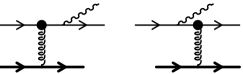
Figure 2: The relevant diagrams for $qA\to q\gamma^{*}X$ in the Color Glass Condensate model. The black dots denote the eikonal interaction between the quark or antiquark with the classical color field.

Note that there could a priori be a third diagram with eikonal interactions of the quark both before and after the photon emission. However, this diagrams is in fact strongly suppressed by large energy denominators [23], which simply indicates that by the time the photon has been emitted after a first scattering of the quark off the nucleus, the nucleus is far behind and any further scattering is impossible (in order words, the nucleus is so fast that the photon is emitted outside of the nucleus). This discrepancy between the number of diagrams contributing to both processes is what makes the correspondence between the two non-trivial, and worth checking explicitly. In the CGC model, the $qA\to q\gamma^{*}X$ amplitude is given by

$${\cal M}^{\mu}_{\gamma^{*}}({\boldsymbol{p}}|{\boldsymbol{q}},{\boldsymbol{k}})=i\int d^{2}{\boldsymbol{x}}_{\perp}e^{i({\boldsymbol{q}}_{\perp}+{\boldsymbol{k}}_{\perp}-{\boldsymbol{p}}_{\perp})\cdot{\boldsymbol{x}}_{\perp}}\left(U({\boldsymbol{x}}_{\perp})-1\right)$$

$$\qquad\quad\times\overline{u}({\boldsymbol{q}})\left[\frac{\gamma^{\mu}(\raise 0.6458pt\hbox{$/$}\kern-5.29999pt\hbox{$Q$}+\raise 0.6458pt\hbox{$/$}\kern-5.29999pt\hbox{$K$}+m)\gamma^{-}}{(Q+K)^{2}-m^{2}+i\epsilon}+\frac{\gamma^{-}(\raise 0.6458pt\hbox{$/$}\kern-5.29999pt\hbox{$P$}-\raise 0.6458pt\hbox{$/$}\kern-5.29999pt\hbox{$K$}+m)\gamma^{\mu}}{(P-K)^{2}-m^{2}+i\epsilon}\right]u({\boldsymbol{p}})\;,$$ (17)

where the two terms correspond to the two diagrams of figure 2 respectively. In this equation $p,q$ and $k$ are the momenta of the incoming quark, and of the outgoing quark and photon respectively, and ${\boldsymbol{x}}_{\perp}$ is the transverse coordinate of the quark. Using now the first of Eqs. (4) as well as

$$u({\boldsymbol{p}})=\frac{1}{2p^{-}}(m+\raise 0.6458pt\hbox{$/$}\kern-5.29999pt\hbox{$P$})\gamma^{-}u({\boldsymbol{p}})\;,$$ (18)

and introducing again a dummy variable ${\boldsymbol{l}}_{\perp}$, we can after some algebra rewrite the $\gamma^{*}$ production amplitude as:

$${\cal M}^{\mu}_{\gamma^{*}}({\boldsymbol{p}}|{\boldsymbol{q}},{\boldsymbol{k}})=\frac{i}{2}\int\frac{d^{2}{\boldsymbol{l}}_{\perp}}{(2\pi)^{2}}\int d^{2}{\boldsymbol{x}}_{1\perp}d^{2}{\boldsymbol{x}}_{2\perp}$$

$$\qquad\;\times e^{i{\boldsymbol{l}}_{\perp}\cdot{\boldsymbol{x}}_{1\perp}}e^{i({\boldsymbol{q}}_{\perp}+{\boldsymbol{k}}_{\perp}-p_{\perp}-l_{\perp})\cdot{\boldsymbol{x}}_{2\perp}}\left(U({\boldsymbol{x}}_{1\perp})-U({\boldsymbol{x}}_{2\perp})\right)$$

$$\qquad\;\times\overline{u}({\boldsymbol{q}})\,\Gamma^{\mu}(-k^{\pm},-{\boldsymbol{k}}_{\perp}|q^{-},-p^{-},{\boldsymbol{q}}_{\perp}-{\boldsymbol{l}}_{\perp})\,u({\boldsymbol{p}})\;,$$ (19)

where $\Gamma^{\mu}$ is again the function defined by Eq. (6). We see that the only difference between the DIS and $\gamma^{*}$-production amplitudes, besides the obvious changes $P\to-P$ and $K\to-K$, is an extra factor $U^{\dagger}({\boldsymbol{x}}_{2\perp})$ under the integral. In other words, the two amplitudes can be related by crossing symmetry up to a unitary matrix, which violates a strict crossing symmetry at the amplitude level. This has been noted independently by S. Peigné in [38], where Drell-Yan and DIS are compared up to the terms involving three scatterings on the target. In the present case, this violation is in fact due to the eikonal approximation. Indeed, this approximation being valid for an asymptotically large relative momentum between the projectile and the target, it does not allow to reverse continuously the momentum of the projectile.

3.2 Cross-section

The photon production cross-section is obtained from the amplitude by

$$d\sigma_{\gamma^{*}}=\frac{d^{3}{\boldsymbol{q}}}{(2\pi)^{2}2q_{0}}\frac{d^{3}{\boldsymbol{k}}}{(2\pi)^{3}2k_{0}}\frac{1}{2p^{-}}2\pi\delta(p^{-}-q^{-}-k^{-})$$

$$\qquad\qquad\times\frac{1}{2N_{c}}\left<{\cal M}^{\mu}_{\gamma^{*}}({\boldsymbol{p}}|{\boldsymbol{q}},{\boldsymbol{k}}){\cal M}^{\nu*}_{\gamma^{*}}({\boldsymbol{p}}|{\boldsymbol{q}},{\boldsymbol{k}})\right>_{\rho}\epsilon_{\mu}(K)\epsilon_{\nu}^{*}(K)\;,$$ (20)

where the factor $1/2N_{c}$ is for the average over the color and spin of the incoming quark. At this point, it is useful to replace the integration variable ${\boldsymbol{l}}_{\perp}$ by ${\boldsymbol{m}}_{\perp}={\boldsymbol{q}}_{\perp}-{\boldsymbol{l}}_{\perp}$ both in the amplitude and in its complex conjugate, in order to exploit the momentum dependence of the function $\Gamma^{\mu}$. Another simplification comes from the fact that any term in the amplitude squared depends non-trivially only on two out of the four transverse coordinates. Therefore, the two transverse coordinates that appear only in exponentials can be integrated out immediately, which gives two delta constraints on some combination of transverse momenta, that can be used in order to perform the integrals over ${\boldsymbol{m}}_{\perp}$ and ${\boldsymbol{m}}^{\prime}_{\perp}$. Following this procedure, one obtains the following form for the differential $\gamma^{*}$ production cross-section:

$$d\sigma_{\gamma^{*}}=\frac{d^{3}{\boldsymbol{q}}}{(2\pi)^{3}2q_{0}}\frac{d^{3}{\boldsymbol{k}}}{(2\pi)^{3}2k_{0}}\frac{1}{2p^{-}}2\pi\delta(p^{-}-q^{-}-k^{-})\,$$

$$\!\!\!\!\times\int d^{2}{\boldsymbol{r}}_{\perp}e^{i({\boldsymbol{q}}_{\perp}+{\boldsymbol{k}}_{\perp}-{\boldsymbol{p}}_{\perp})\cdot{\boldsymbol{r}}_{\perp}}\int d^{2}{\boldsymbol{X}}_{\perp}{\rm Tr}_{c}\left<1-U({\boldsymbol{X}}_{\perp}+\frac{{\boldsymbol{r}}_{\perp}}{2})U^{\dagger}({\boldsymbol{X}}_{\perp}-\frac{{\boldsymbol{r}}_{\perp}}{2})\right>_{\rho}$$

$$\!\!\!\!\times\frac{1}{2N_{c}}\Big{[}M({\boldsymbol{p}}_{\perp}-{\boldsymbol{k}}_{\perp},{\boldsymbol{p}}_{\perp}-{\boldsymbol{k}}_{\perp})+M({\boldsymbol{q}}_{\perp},{\boldsymbol{q}}_{\perp})$$

$$\quad-M({\boldsymbol{q}}_{\perp},{\boldsymbol{p}}_{\perp}-{\boldsymbol{k}}_{\perp})-M({\boldsymbol{p}}_{\perp}-{\boldsymbol{k}}_{\perp},{\boldsymbol{q}}_{\perp})\Big{]}\;,$$ (21)

where we use the shorthand

$$M({\boldsymbol{m}}_{\perp},{\boldsymbol{m}}^{\prime}_{\perp})\equiv\epsilon_{\mu}(K)\epsilon^{*}_{\nu}(K)\;{\rm Tr}_{d}\big{(}(\raise 0.43057pt\hbox{$/$}\kern-6.30005pt\hbox{$q$}+m)\Gamma^{\mu}(-k^{\pm},-{\boldsymbol{k}}_{\perp}|q-,-p^{-},{\boldsymbol{m}}_{\perp})$$

$$\qquad\qquad\qquad\qquad\times(\raise 0.43057pt\hbox{$/$}\kern-6.30005pt\hbox{$p$}+m)\Gamma^{\nu\dagger}(-k^{\pm},-{\boldsymbol{k}}_{\perp}|q^{-},-p^{-},{\boldsymbol{m}}^{\prime}_{\perp})\big{)}\;.$$ (22)

In fact, the four terms in Eq. (21) could have been obtained directly by squaring the two terms of Eq. (17). Again, we see that the dipole cross-section appears naturally in this cross-section. Therefore, if one determines the dipole cross-section from DIS data, then it becomes possible to make quantitative predictions for the production of virtual photons in pA collisions. This possibility has already been exploited in [26] in order to study nuclear effects on the Drell-Yan process.

One can in fact obtain a form very similar to Eq. (11) for the $\gamma^{*}$ production cross-section integrated over the transverse momenta ${\boldsymbol{q}}_{\perp}$ and ${\boldsymbol{k}}_{\perp}$ of the final particles:

$$\sigma_{\gamma^{*}}=\int_{0}^{1}dz\int d^{2}{\boldsymbol{r}}_{\perp}\left|\phi(p^{-},{\boldsymbol{p}}_{\perp}|k^{+},z,{\boldsymbol{r}}_{\perp})\right|^{2}\sigma_{\rm dipole}({\boldsymbol{r}}_{\perp})\;,$$ (23)

where $z$ is the longitudinal momentum fraction taken by the photon ($k^{-}=zp^{-}$, $q^{-}=(1-z)p^{-}$) and where we denote

$$\left|\phi(p^{-},{\boldsymbol{p}}_{\perp}|k^{+},z,{\boldsymbol{r}}_{\perp})\right|^{2}\equiv\frac{1}{64\pi p_{-}^{2}z(1-z)}\int\frac{d^{2}{\boldsymbol{q}}_{\perp}}{(2\pi)^{2}}\int\frac{d^{2}{\boldsymbol{k}}_{\perp}}{(2\pi)^{2}}e^{i({\boldsymbol{q}}_{\perp}+{\boldsymbol{k}}_{\perp}-{\boldsymbol{p}}_{\perp})\cdot{\boldsymbol{r}}_{\perp}}$$

$$\qquad\times\Big{[}M({\boldsymbol{p}}_{\perp}-{\boldsymbol{k}}_{\perp},{\boldsymbol{p}}_{\perp}-{\boldsymbol{k}}_{\perp})+M({\boldsymbol{q}}_{\perp},{\boldsymbol{q}}_{\perp})$$

$$\qquad\quad-M({\boldsymbol{q}}_{\perp},{\boldsymbol{p}}_{\perp}-{\boldsymbol{k}}_{\perp})-M({\boldsymbol{p}}_{\perp}-{\boldsymbol{k}}_{\perp},{\boldsymbol{q}}_{\perp})\Big{]}\;.$$ (24)

4 Forward pion production in pA collisions

4.1 Quark scattering amplitude

In this section we show how one can relate the cross section for forward particle production in pA collisions to the dipole cross-section. To be specific, we will consider pions but this can be repeated for any particle for which there is a known fragmentation function. We will use the results of [21, 22] for scattering of an on-shell quark from the target described by the Color Glass Condensate.

Figure 3: The relevant diagram for $qA\to qX$ in the Color Glass Condensate model. The black dots denote the eikonal interaction between the quark or antiquark with the classical color field.

The amplitude for scattering of a quark from the target described by a classical field is given by the diagram represented in figure 3, and has been obtained in [21, 22]. Factoring out the obvious $2\pi\delta(p^{-}-q^{-})$, this amplitude reads (the same as Eq. (1)):

$${\cal M}_{qA\to qX}({\boldsymbol{p}}|{\boldsymbol{q}})=\overline{u}({\boldsymbol{q}})\left[\gamma^{-}\int d^{2}{\boldsymbol{x}}_{\perp}e^{i({\boldsymbol{q}}_{\perp}-{\boldsymbol{p}}_{\perp})\cdot{\boldsymbol{x}}_{\perp}}(U({\boldsymbol{x}}_{\perp})-1)\right]u({\boldsymbol{p}})\;,$$ (25)

where ${\boldsymbol{p}}$ and ${\boldsymbol{q}}$ are the momenta of the incoming and outgoing quark respectively.

4.2 Scattering cross section

From this amplitude, it is easy to obtain the cross section [21, 22]:

$$d\sigma_{qA\to qX}=\frac{d^{3}{\boldsymbol{q}}}{(2\pi)^{3}2q_{0}}\frac{1}{2p^{-}}2\pi\delta(p^{-}-q^{-})\frac{1}{2N_{c}}\left<{\cal M}_{qA\to qX}({\boldsymbol{p}}|{\boldsymbol{q}}){\cal M}^{*}_{qA\to qX}({\boldsymbol{p}}|{\boldsymbol{q}})\right>_{\rho}\;,$$ (26)

where the prefactor $1/2N_{c}$ comes from the average over the spin and color of the incoming quark. This can be rewritten as:

$$d\sigma_{qA\to qX}=\frac{d^{2}{\boldsymbol{q}}_{\perp}}{(2\pi)^{2}}\frac{1}{N_{c}}\int d^{2}{\boldsymbol{r}}_{\perp}e^{i({\boldsymbol{q}}_{\perp}-{\boldsymbol{p}}_{\perp})\cdot{\boldsymbol{r}}_{\perp}}$$

$$\qquad\times\int d^{2}{\boldsymbol{X}}_{\perp}{\rm Tr}_{c}\left<\left(U({\boldsymbol{X}}_{\perp}+\frac{{\boldsymbol{r}}_{\perp}}{2})-1\right)\left(U^{\dagger}({\boldsymbol{X}}_{\perp}-\frac{{\boldsymbol{r}}_{\perp}}{2})-1\right)\right>_{\rho}\;.$$ (27)

Note that for the scattering of a gluon, one would have to replace the matrix $U$ by its analogue in the adjoint representation, but the average over the color of the initial state would require a factor $1/(N_{c}^{2}-1)$ instead of $1/N_{c}$. Expanding the correlator in the bracket $\left<\cdots\right>_{\rho}$, we can rewrite this cross-section in terms of the dipole cross-section:

$$d\sigma_{qA\to qX}=\frac{d^{2}{\boldsymbol{q}}_{\perp}}{(2\pi)^{2}}\,dq^{-}\delta(q^{-}-p^{-})\int d^{2}{\boldsymbol{r}}_{\perp}e^{i{\boldsymbol{q}}_{\perp}\cdot{\boldsymbol{r}}_{\perp}}$$

$$\!\!\!\!\times\left[\frac{1}{N_{c}}\int d^{2}{\boldsymbol{X}}_{\perp}{\rm Tr}_{c}\left<2-U({\boldsymbol{X}}_{\perp}+\frac{{\boldsymbol{r}}_{\perp}}{2})-U^{\dagger}({\boldsymbol{X}}_{\perp}-\frac{{\boldsymbol{r}}_{\perp}}{2})\right>_{\rho}-\sigma_{\rm dipole}({\boldsymbol{r}}_{\perp})\right]\;,$$

where, anticipating the use of collinear factorization for the incoming quark, we have set ${\boldsymbol{p}}_{\perp}=0$. The first term $\left<2-U-U^{\dagger}\right>_{\rho}$ is essential in order to obtain the correct total cross-section. Indeed, integrating over ${\boldsymbol{q}}_{\perp}$ generates a $\delta({\boldsymbol{r}}_{\perp})$, and since $\sigma_{\rm dipole}({\boldsymbol{r}}_{\perp}=0)=0$, we have for the total $qA\to qX$ cross-section:

$$\sigma_{qA\to qX}^{\rm total}=\frac{1}{N_{c}}\int d^{2}{\boldsymbol{X}}_{\perp}{\rm Tr}_{c}\left<2-U({\boldsymbol{X}}_{\perp})-U^{\dagger}({\boldsymbol{X}}_{\perp})\right>_{\rho}\;.$$ (30)

If we recall (see [27] for instance) that $\left<U({\boldsymbol{x}}_{\perp})\right>_{\rho}$ is suppressed exponentially like $\exp(-Q_{s}^{2}/\Lambda_{{}_{QCD}}^{2})$ when $Q_{s}\gg\Lambda_{{}_{QCD}}$, we can approximate the $qA\to qX$ cross-section by:

$$d\sigma_{qA\to qX}=\frac{d^{2}{\boldsymbol{q}}_{\perp}}{(2\pi)^{2}}\,dq^{-}\delta(q^{-}-p^{-})\int d^{2}{\boldsymbol{r}}_{\perp}e^{i{\boldsymbol{q}}_{\perp}\cdot{\boldsymbol{r}}_{\perp}}(2\pi R^{2}-\sigma_{\rm dipole}({\boldsymbol{r}}_{\perp}))\;,$$

(31)

for a target of radius $R$. The term in $2\pi R^{2}$ contributes only to the scattering in the forward direction (i.e. at ${\boldsymbol{q}}_{\perp}=0$).

4.3 Discussion

4.3.1 Cronin effect at the partonic level

From the previous relations, it is trivial to write the non-forward part of the $q_{\perp}$-spectrum as:

$$\frac{d\sigma_{qA\to qX}}{d^{2}{\boldsymbol{q}}_{\perp}}=-\frac{1}{(2\pi)^{2}}\,\widetilde{\sigma}_{\rm dipole}(q_{\perp})\;,$$ (32)

where $\widetilde{\sigma}_{\rm dipole}(q_{\perp})$ is the Fourier transform of the dipole cross-section, defined as:

$$\widetilde{\sigma}_{\rm dipole}(q_{\perp})\equiv\int d^{2}{\boldsymbol{r}}_{\perp}e^{i{\boldsymbol{q}}_{\perp}\cdot{\boldsymbol{r}}_{\perp}}\sigma_{\rm dipole}({\boldsymbol{r}}_{\perp})\;.$$ (33)

In other words, the $q_{\perp}$-spectrum of particle production in $pA$ collisions is given by the opposite of the Fourier transform of the dipole cross-section.

In the McLerran-Venugopalan model, this Fourier transform has been studied in detail in [27, 28] where it controls the production of $q\bar{q}$ pairs in ultra-peripheral $AA$ collisions and was denoted $\pi R^{2}C({\boldsymbol{q}}_{\perp})$ (see for instance the appendix B of [27]). In particular, the large $q_{\perp}$ behavior of this function was found to be

$$C({\boldsymbol{q}}_{\perp})=2{{Q_{s}^{2}}\over{q_{\perp}^{4}}}+{8\over\pi}{{Q_{s}^{4}}\over{q_{\perp}^{6}}}\left(\ln\left({{q_{\perp}}\over{\Lambda_{{}_{QCD}}}}\right)-1\right)+{\cal O}\left({{Q_{s}^{6}}\over{q_{\perp}^{8}}}\right)\;.$$ (34)

Note that if one replaces $Q_{s}^{2}$ by its expression in terms of parton distributions inside the target, the first term in $1/q_{\perp}^{4}$ reproduces the perturbative QCD result for $qg\to qg$ scattering with one gluon exchange in the t-channel (i.e. the dominant piece at high energy). In addition, if one assumes that $Q_{s}^{2}$ scales like $A^{1/3}$ for large nuclei, then the leading term of the $q_{\perp}$ spectrum simply scales like $A$ (another $A^{2/3}$ comes from the transverse area $\pi R^{2}$). If the second term in this expansion scales differently with $A$, then there is a Cronin effect. From Eq. (34), one can see that the next-to-leading term in the $q_{\perp}$-spectrum is scaling like $A^{4/3}$ and is positive. Therefore, one has a positive Cronin effect in the McLerran-Venugopalan model.

Figure 4: Cronin effect at the partonic level in the McLerran-Venugopalan model. The reference nucleus is chosen such that the corresponding saturation scale is $Q_{s}^{2}{}_{\rm ref}=1$GeV². This reference value of $Q_{s}$ is compared to nuclei for which $Q_{s}^{2}=2$ GeV² and $Q_{s}^{2}=3$ GeV². The infrared cutoff is set to $\Lambda=200$ MeV.

The ratio $(A_{\rm ref}/A)d\sigma_{qA\to qX}/d\sigma_{qA_{\rm ref}\to qX}$, as predicted in the McLerran-Venugopalan model, is plotted as a function of $q_{\perp}$ in figure 4. The reference nucleus is chosen such that the corresponding saturation scale is $Q_{s}^{2}{}_{\rm ref}=1~{}$GeV², and the ratio is displayed for two nuclei such that the saturation scales are $Q_{s}^{2}=2$ GeV² and $Q_{s}^{2}=3$ GeV². One can see that this ratio goes to $1$ at large transverse momentum, and exhibits a pronounced maximum at intermediate $q_{\perp}$’s before dropping below $1$ at small transverse momenta.

Alternatively, one could take $A_{ref}=A=200$ and consider quark nucleus scattering at mid rapidity, assuming that $Q_{s}^{2}{}_{\rm ref}=1~{}$GeV² at mid rapidity. Then the solid and dashed lines correspond to the relative enhancement of the cross section in the forward rapidity region, $y\sim 2.5$ and $y\sim 3.5$ units away from mid rapidity (towards the proton), respectively. The low $q_{\perp}$ spectrum is more suppressed as one goes to more forward rapidities and high $q_{\perp}$ enhancement is stronger and moves to higher $q_{\perp}$.

It would be interesting to study whether this phenomenon is present in more sophisticated models of the dipole cross-section, like the model of Bartels, Golec-Biernat and Kowalski. It is also necessary to fold this “partonic level” calculation with the proton parton distribution functions, and with the appropriate fragmentation functions, as this could potentially suppress the effect. A numerical study of these issues is underway.

4.3.2 Further constraints of the dipole cross-section in pA

In DIS, one does not probe thoroughly the dipole cross-section, but only its overlap with the square of the photon wave function. This implies that some values of $r_{\perp}$ matter more than others in the integral. One could therefore see Eq. (32) as another way of constraining the dipole cross-section. In particular, one would like to recover the results of perturbative QCD at large $q_{\perp}$, that is a cross-section that falls like $q_{\perp}^{-4}$ (up to logarithms coming from the running $\alpha_{s}$ and from the DGLAP evolution of the gluon distribution inside the target).

For instance, this remark pretty much excludes the Golec-Biernat-Wüsthoff model of the dipole cross-section. Indeed, in this model (see Eq. (15)) the Fourier transform that gives the $q_{\perp}$-spectrum can be performed analytically, giving:

$$\frac{d\sigma_{qA\to qX}}{d^{2}{\boldsymbol{q}}_{\perp}}=\frac{R_{0}^{2}(x)\sigma_{0}}{\pi}\,e^{-R_{0}^{2}(x)q_{\perp}^{2}}.$$ (35)

The major difference compared to the result in the McLerran-Venugopalan model is the large $q_{\perp}$ behavior, which exhibits a Gaussian tail, as opposed to a power law tail. This fact alone is probably enough to justify not considering this model any further in order to study the region of large transverse momenta in pA collisions.

For the Bartels-Golec-Biernat-Kowalski model, one needs to compute numerically the Fourier transform of the dipole cross-section. In order to do this, we have taken the parameters of their second fit (“Fit 2” in Table 1 of [35]), which lead to the results displayed in figure 5.

Figure 5: Values of $-q_{\perp}^{4}\widetilde{\sigma}_{\rm dipole}(q_{\perp})$ as a function of $q_{\perp}$, for several values of $x$ in the model of Bartels, Golec-Biernat and Kowalski.

One can see that for very small values of $x$ ($x=10^{-4},x=10^{-5}$ on this plot) one obtains the expected scaling at large $q_{\perp}$. Indeed, $q_{\perp}^{4}$ times the Fourier transform of the dipole cross section is almost constant. However, for larger values of $x$ ($x=10^{-2},x=10^{-3}$ on the plot), the Fourier transform of the dipole cross-section suddenly drops at some $q_{\perp}$ and its sign changes .

Above the $q_{\perp}$ where this happens, one would obtain a negative $qA\to qX$ cross-section from formula Eq. (32). In this formula, one apparently probes different aspects of the dipole cross-section compared to DIS, and the model by Bartels, Golec-Biernat and Kowalski, although very successful at fitting all the HERA DIS data at $x<10^{-2}$, does not give a consistent answer for pA collisions at moderate $x$. Somehow, this defect is hidden in DIS by the way the photon wave functions weights the different values of $r_{\perp}$. Given this, one could perhaps reverse the main argument of this paper, and consider pA collisions as a way of either fine tuning the dipole model, or as a way of ruling it out.

4.4 From $qA\to qX$ to $pA\to\pi X$

To relate (31) to proton-nucleus collisions, we can use collinear factorization on the proton side and convolute (31) with the quark distribution function inside a proton and a quark-pion fragmentation function to get the cross section for $pA\rightarrow\pi X$.

$${d\sigma_{pA\to\pi(k)X}\over dk^{-}d^{2}{\boldsymbol{k}}_{\perp}}\equiv\int dx_{q}\,dz\,q_{p}(x_{q})\,\,{d\sigma_{qA\to qX}\over dq^{-}d^{2}{\boldsymbol{q}}_{\perp}}\,\,D_{q/\pi}(z)$$ (36)

where $q_{p}(x_{q})$ is the distribution function of quarks with fractional momentum $x_{q}$ inside a proton and $D_{q/\pi}(z)$ is the fragmentation function of a quark into a pion carrying fraction $z$ of its energy. Using (31) in (36) we get

$${d\sigma_{pA\to\pi(y,{\boldsymbol{k}}_{\perp})X}\over dyd^{2}{\boldsymbol{k}}_{\perp}}={1\over(2\pi)^{2}}\sqrt{k_{\perp}^{2}\over s}\,e^{y}\,\int_{z_{\rm min}}^{1}dz\,q_{p}\left(x_{q}\right)\,D_{q/\pi}(z)$$

$$\qquad\times\int d^{2}{\boldsymbol{r}}_{\perp}e^{i{\boldsymbol{k}}_{\perp}\cdot{\boldsymbol{r}}_{\perp}/z}(2\pi R^{2}-\sigma_{\rm dipole}({\boldsymbol{r}}_{\perp},x_{g}))\;,$$ (37)

where we have used the following kinematical relations $x_{q}=k_{\perp}e^{y}/z\sqrt{s}$, $x_{g}=k_{\perp}e^{-y}/z\sqrt{s}$, $z_{\rm min}=k_{\perp}e^{y}/\sqrt{s}$ ($\sqrt{s}$ is the center of mass energy for a proton-nucleon subsystem). This way one can relate production of pions, kaons, protons, neutrons, photons and dileptons in proton-nucleus collisions in the forward rapidity region to the structure functions measured in DIS. For this approach to be self-consistent, one needs to make sure that the dominant contribution to (37) comes from the small $x$ ($\leq 0.01$) region. Our preliminary result seem to indicate that this is indeed the case. A detailed numerical study of particle production in proton-nucleus collisions at RHIC is currently underway and will be reported elsewhere.

5 Conclusions

In this paper, we have shown that in a classical description of the gluon content of the nucleus, there are many interesting physical quantities that can be related to the dipole cross-section (or, at a more formal level, to the correlator $\left<U(0)U^{\dagger}({\boldsymbol{x}}_{\perp})\right>$ of two Wilson lines). This was already known for deep inelastic scattering and for the Drell-Yan process when one considers cross-sections integrated over the phase-space of the final state. In this paper, we establish also a similar correspondence for forward particle production in proton nucleus collisions, this time for the differential cross-section. More precisely, we show that the $q_{\perp}$ spectrum of the produced particles is related to the Fourier transform of the dipole cross-section.

At a more formal level, we have generalized the standard leading twist collinear factorization approach to calculation of hadronic cross sections by showing that there is a universal object, the quark antiquark dipole cross section, which appears in all particle production cross sections in high energy proton-nucleus collisions. This dipole cross section plays the role of leading twist parton distributions in an all twist environment. In principle, it can be measured in DIS or for example, in single inclusive pion production in high energy proton-nucleus collisions. Once it is measured in a given process, it can be used to predict cross sections for other processes such as single inclusive hadron, jet, photon or dilepton production in high energy proton-nucleus collisions.

This result could therefore be used in order to make predictions for pA collisions, or to further constrain (or to rule out) the dipole model with proton-nucleus experiments. The detailed numerical study needed in order to make quantitative statements is in progress and will be presented in a future work [40]. However, a preliminary investigation of the Fourier transform of the dipole cross-section in the model of [35] seem to lead to a negative $qA\to qX$ differential cross-section for some values of $x$ at large $q_{\perp}$. This suggests that the small $r_{\perp}$ improvement of the dipole cross-section made in [35] over [32, 33] is still not quite able to ensure that the results of perturbative QCD are recovered at large transverse momentum.

References

- [1] L.V. Gribov, E.M. Levin, M.G. Ryskin, Phys. Rept. 100, 1 (1983).
- [2] A.H. Mueller, J-W. Qiu, Nucl. Phys. B 268, 427 (1986).
- [3] L. McLerran, R. Venugopalan, Phys. Rev. D 49, 2233 (1994).
- [4] L. McLerran, R. Venugopalan, Phys. Rev. D 49, 3352 (1994).
- [5] L. McLerran, R. Venugopalan, Phys. Rev. D 59, 094002 (1999).
- [6] Yu.V. Kovchegov, Phys. Rev. D 54, 5463 (1996).
- [7] Yu.V. Kovchegov, Phys. Rev. D 55, 5445 (1997).
- [8] J. Jalilian-Marian, A. Kovner, L. McLerran, H. Weigert, Phys. Rev. D 55, 5414 (1997).
- [9] J. Jalilian-Marian, A. Kovner, A. Leonidov, H. Weigert, Nucl. Phys. B 504, 415 (1997).
- [10] J. Jalilian-Marian, A. Kovner, A. Leonidov, H. Weigert, Phys. Rev. D 59, 014014 (1999).
- [11] J. Jalilian-Marian, A. Kovner, A. Leonidov, H. Weigert, Phys. Rev. D 59, 034007 (1999).
- [12] J. Jalilian-Marian, A. Kovner, H. Weigert, Phys. Rev. D 59, 014015 (1999).
- [13] A. Ayala, J. Jalilian-Marian, L. McLerran, R. Venugopalan, Phys. Rev. D 52, 2935 (1995).
- [14] A. Ayala, J. Jalilian-Marian, L. McLerran, R. Venugopalan, Phys. Rev. D 53, 458 (1996).
- [15] A. Kovner, G. Milhano, Phys. Rev. D 61, 014012 (2000).
- [16] A. Kovner, G. Milhano, H. Weigert, Phys. Rev. D 62, 114005 (2000).
- [17] E. Iancu, A. Leonidov, L. McLerran, Nucl. Phys. A 692, 583 (2001).
- [18] E. Iancu, A. Leonidov, L. McLerran, Phys. Lett. B 510, 133 (2001).
- [19] E. Iancu, L. McLerran, Phys. Lett. B 510, 145 (2001).
- [20] E. Ferreiro, E. Iancu, A. Leonidov, L. McLerran, Nucl. Phys. A 703, 489 (2002).
- [21] A. Dumitru, J. Jalilian-Marian, Phys. Rev. Lett. 89, 022301 (2002).
- [22] A. Dumitru, J. Jalilian-Marian, Phys. Lett. B 547, 15 (2002).
- [23] F. Gelis, J. Jalilian-Marian, Phys. Rev. D 66, 014021 (2002).
- [24] F. Gelis, J. Jalilian-Marian, hep-ph/0208141, to appear in Phys. Rev. D .
- [25] B.Z. Kopeliovich, J. Raufeisen, A.V. Tarasov, Phys. Lett. B 503, 91 (2001).
- [26] B.Z. Kopeliovich, J. Raufeisen, A.V. Tarasov, M.B. Johnson, hep-ph/0110221 .
- [27] F. Gelis, A. Peshier, Nucl. Phys. A 697, 879 (2002).
- [28] F. Gelis, A. Peshier, Nucl. Phys. A 707, 175 (2002).
- [29] E. Ferreiro, E. Iancu, K. Itakura, L. McLerran, Nucl. Phys. A 710, 373 (2002).
- [30] A.H. Mueller, Nucl. Phys. B 558, 285 (1999).
- [31] Yu.V. Kovchegov, Phys. Rev. D 60, 034008 (1999).
- [32] K. Golec-Biernat, M. Wusthoff, Phys. Rev. D 59, 014017 (1999).
- [33] K. Golec-Biernat, M. Wusthoff, Phys. Rev. D 60, 114023 (1999).
- [34] K. Golec-Biernat, M. Wusthoff, Eur. Phys. J. C 20, 313 (2001).
- [35] J. Bartels, K. Golec-Biernat, H. Kowalski, Phys. Rev. D 66, 014001 (2002).
- [36] A.H. Mueller, Nucl. Phys. B 335, 115 (1990).
- [37] K.J. Eskola, V.J. Kolhinen, C.A. Salgado, Eur. Phys. J. C 9, 61 (1999).
- [38] S. Peigné, hep-ph/0206138.
- [39] H. Kowalski, private communication.
- [40] F. Gelis, J. Jalilian-Marian, work in progress.